


 Abstract
 HTML
 Reference
 Related
 PDF



-
The transport properties of nuclear matter, such as shear viscosity, thermal conductivity, and diffusion coefficients, play a fundamental role in both nuclear reaction dynamics [1−3] and astrophysical phenomena [4, 5]. In heavy-ion collisions, transport coefficients enter dynamical simulations explicitly and affect the extraction of the EOS [6, 7]. In neutron stars, they influence thermal evolution [8] and r-mode oscillations [9]. A reliable microscopic determination of transport coefficients is therefore essential for interpreting data from both terrestrial experiments and astronomical observations.
Among these quantities, the isospin diffusion coefficient characterizes the relaxation of composition gradients and is closely related to the nuclear symmetry energy, the part of the EOS that quantifies the energy cost of isospin asymmetry [10−12]. In heavy-ion collisions, isospin diffusion has been identified as one of the most sensitive probes of the density dependence of the symmetry energy [2, 3, 13, 14]. The significance of the symmetry energy stems from its important role in understanding many aspects of nuclear physics, including nuclear structure, reaction dynamics, neutron star physics, and r-process nucleosynthesis [15−20]. However, its density dependence, particularly away from saturation density, remains one of the major uncertainties in the EOS [21−27]. Since the extraction of symmetry-energy constraints from reaction observables depends sensitively on the transport coefficients adopted in simulations, a quantitatively reliable determination of the isospin diffusion coefficient is indispensable. In addition, isospin diffusion provides information on nuclear stopping power and tests the assumption of global equilibrium commonly employed in statistical multifragmentation models [1, 7].
The theoretical framework for calculating transport coefficients in degenerate Fermi systems was established by Abrikosov and Khalatnikov (AK) within Landau Fermi-liquid theory [28]. Exact solutions for single-component systems were later obtained by Brooker and Sykes [29] and by Højgaard Jensen et al. [30]. Flowers and Itoh [5] pioneered the extension to multicomponent Fermi liquids, and Anderson [31] subsequently formulated exact integral equations for the multicomponent case. In nuclear matter applications, early calculations were based on free-space nucleon–nucleon scattering amplitudes [5], thereby neglecting medium and many-body effects. Medium modifications were later incorporated using correlated basis function (CBF) methods [32, 33] and the Brueckner–Hartree–Fock (BHF) approach [34−37]. A comparison between CBF and BHF G-matrix calculations in pure neutron matter showed overall consistency [38], although it was later pointed out [39] that a numerical factor was missing in Ref. [38]. In general, existing calculations of transport coefficients in nuclear matter agree at the order-of-magnitude level but exhibit noticeable quantitative differences. These discrepancies may arise from several sources: incomplete numerical factors in the AK formalism, approximate treatments of the kinetic equation (such as retaining only the leading term in the series expansion), and simplified treatments of medium effects, for example, modeling in-medium cross sections solely through effective-mass scaling. Recent developments in ab initio approaches [40], together with increasingly microscopic determinations of in-medium cross sections [41], provide more reliable inputs for transport coefficients and may help reduce the uncertainties associated with medium effects. Additional variations stem from differences in the underlying nuclear interactions, particularly in the implementation of three-body forces. Although the leading-term approximation has been shown to be reliable for shear viscosity and thermal conductivity [36, 39], its validity for the diffusion coefficient remains to be clarified. Moreover, the isospin-asymmetry dependence of the diffusion coefficient is often assumed to follow a simple quadratic form [13], the reliability of which requires further scrutiny.
In view of these issues, and given the important role of the isospin diffusion coefficient in heavy-ion collision simulations and in constraining the nuclear symmetry energy, we perform a systematic and self-consistent investigation of the isospin diffusion coefficients within the AK framework. The key microscopic inputs, including the susceptibility, effective masses, and in-medium differential cross sections, are calculated consistently within the BHF approach using the Argonne v18 interaction, with and without the inclusion of a microscopic three-body force (3BF) [42−44].
The paper is organized as follows. In Sec. II, we outline the theoretical formalism for diffusion coefficients in binary Fermi liquids and the microscopic inputs within the BHF approach. Section III presents the numerical results and discussion. A summary is given in Sec. IV.
-
The transport properties of normal Fermi liquids in the low-temperature limit are well described by the AK theory of Landau Fermi liquids [45]. The formalism for a one-component system was first derived by Abrikosov and Khalatnikov [28]. Its extension to multicomponent systems was developed in Refs. [5, 31]. In the following, we closely follow the formalism of Refs. [5, 31] and briefly outline the expressions required to obtain the diffusion coefficient.
-
For nuclear matter with neutron number density
$ \rho_n $ and proton number density$ \rho_p $ , the relevant flux for the relative diffusion of neutrons and protons is the number current,$ \begin{split} {\boldsymbol{J}}_{\tau}=\sum_{{\boldsymbol{p}}\sigma}{\boldsymbol{v}}_{\tau}\delta n_{{\boldsymbol{p}}\tau}, \end{split} $
(1) with
$ \tau=n,p $ representing neutrons and protons,$ \delta n_{{\boldsymbol{p}}\tau}= n_{{\boldsymbol{p}}\tau}-n^0_{{\boldsymbol{p}}\tau} $ measures the deviation of the perturbed distribution$ n_{{\boldsymbol{p}}\tau} $ from the equilibrium distribution$ n^0_{{\boldsymbol{p}}\tau}= $ $ \big(1+{\mathrm{e}}^{\frac{\epsilon_{{\boldsymbol{p}}\tau}-\mu_\tau}{k_BT}}\big)^{-1} $ . The summation over σ contributes only a factor of 2 arising from spin degeneracy. Moreover,$ {\boldsymbol{v}}_{\tau}={\boldsymbol{p}}_{\tau}/m^*_{\tau} $ is the velocity, where$ m^*_\tau $ denotes the effective mass of nucleons with isospin τ. Although spin polarization of about 1%~2% may occur in intermediate-energy heavy-ion collisions [46], the present work focuses exclusively on isospin diffusion. Note that this particle flux generally contains contributions from both diffusion and bulk motion. Consequently, the bulk-motion contribution must be subtracted to evaluate diffusion. The current resulting from diffusion can be defined as$ \begin{split} ({\boldsymbol{J}}_{\tau})_{{\rm{diff}}}={\boldsymbol{J}}_{\tau}-\bar{{\boldsymbol{v}}}\rho_{\tau}, \end{split} $
(2) where
$ \bar{{\boldsymbol{v}}} $ is an average velocity corresponding to the bulk motion. In general,$ \bar{{\boldsymbol{v}}} $ can be chosen so that the diffusive particle flux vanishes, i.e.,$ {\boldsymbol{J}}_{n}+{\boldsymbol{J}}_{p}-\bar{{\boldsymbol{v}}}\rho=0 $ , where$ \rho=\rho_n+\rho_p $ is the total number density. For isospin diffusion, only the difference$ ({\boldsymbol{J}}_{n})_{{\rm{diff}}}-({\boldsymbol{J}}_{p})_{{\rm{diff}}} $ is relevant, and one obtains,$ \begin{split} {\boldsymbol{J}}_{{\rm{diff}}}=({\boldsymbol{J}}_{n})_{{\rm{diff}}}-({\boldsymbol{J}}_{p})_{{\rm{diff}}}=\sum_{{\boldsymbol{p}}\tau}{\boldsymbol{v}}_{\tau}\big(\varsigma_\tau-\beta\big)\delta n_{{\boldsymbol{p}}\tau}. \end{split} $
(3) Here,
$ \varsigma_n = +1 $ ,$ \varsigma_p = -1 $ , and$ \beta=(\rho_n-\rho_p)/\rho $ denotes the isospin asymmetry. The small quantity$ \delta n_{{\boldsymbol{p}}\tau} $ is crucial for determining the transport coefficients, which are obtained from the linearized Landau kinetic equation.$ \begin{split} &-\frac{\partial n^0_{{\boldsymbol{p}}_1\tau}}{\partial x_1}X_{1\tau}(x_1,\hat{{\boldsymbol{p}}}_1)\\ =&-\frac{m^*_{\tau}(k_BT)^2}{8\pi^4\hbar^6}\int {\mathrm{d}}x_3\int {\mathrm{d}}x_4 n^0(x_1)n^0(x_3+x_4-x_1)\\ &\times[1-n^0(x_3)][1-n^0(x_4)]\sum_{\tau'}m^{*2}_{\tau'}\int\frac{{\mathrm{d}}\Omega}{4\pi}\int\frac{{\mathrm{d}}\phi_2}{2\pi}\\ &\times\frac{W_{\tau\tau'}\alpha_{\tau\tau'}}{1+\delta_{\tau\tau'}}\Big[-\Big(\frac{\partial n^0_{{\boldsymbol{p}}_1\tau}}{\partial x_1}\Big)^{-1}\delta n_{{\boldsymbol{p}}_1\tau}-\Big(\frac{\partial n^0_{{\boldsymbol{p}}_2\tau'}}{\partial x_2}\Big)^{-1}\delta n_{{\boldsymbol{p}}_2\tau'} \\ &+\bigg(\frac{\partial n^0_{{\boldsymbol{p}}_3\tau}}{\partial x_3}\bigg)^{-1}\delta n_{{\boldsymbol{p}}_3\tau}+\bigg(\frac{\partial n^0_{{\boldsymbol{p}}_4\tau'}}{\partial x_4}\bigg)^{-1}\delta n_{{\boldsymbol{p}}_4\tau'}\Big]. \end{split} $
(4) Here,
$ X_{1\tau}(x_1,\hat{{\boldsymbol{p}}}_1) $ is the driving term and$ x= (\epsilon_{{\boldsymbol{p}}\tau}-\mu_\tau)/ (k_BT) $ . Note that the integration limits for$ x_3 $ and$ x_4 $ are taken from$ -\infty $ to$ \infty $ . This choice is justified in the low-temperature limit, where small deviations of$ \epsilon_{{\boldsymbol{p}}\tau} $ from the Fermi surface lead to large variations in the variable x. Moreover, in the low-temperature limit, all quasiparticles can be placed on the Fermi surface wherever possible. Quantities such as the scattering momentum, the effective mass, and the velocity in the flux expression (1) are all restricted to the vicinity of the Fermi surface. Indices 1 and 2 (3 and 4) denote incident (outgoing) particles. For convenience, 1 and 3 (2 and 4) can be assumed to belong to the same component, i.e.,$ |{\boldsymbol{p}}_1|=|{\boldsymbol{p}}_3|=p_{\tau} $ ($ |{\boldsymbol{p}}_2|= |{\boldsymbol{p}}_4|=p_{\tau'} $ ), with$ p_{\tau} $ ($ p_{\tau'} $ ) being the Fermi momentum for isospin τ ($ \tau' $ ).$ W_{\tau\tau'}=\sum_{\sigma_2\sigma_3\sigma_4}w_{\tau\tau'} $ denotes the differential transition rate, where$ w_{\tau\tau'} $ is the transition probability for the two quasiparticles to scatter from the initial state$ |{\boldsymbol{p}}_3\sigma_3{\boldsymbol{p}}_4\sigma_4\rangle $ into the final state$ |{\boldsymbol{p}}_1\sigma_1{\boldsymbol{p}}_2\sigma_2\rangle $ .$ W_{\tau\tau'} $ is directly related to the differential nucleon–nucleon cross section and depends on the AK angles θ and ϕ ($ \mathrm{d}\Omega=\sin\theta\mathrm{d}\theta\mathrm{d}\phi $ ), where θ is the angle between$ {\boldsymbol{p}}_1 $ and$ {\boldsymbol{p}}_2 $ , and ϕ is the angle between the$ {\boldsymbol{p}}_1 $ -$ {\boldsymbol{p}}_2 $ and$ {\boldsymbol{p}}_3 $ -$ {\boldsymbol{p}}_4 $ planes.$ \phi_2 $ is the azimuthal angle of$ {\boldsymbol{p}}_2 $ with respect to$ {\boldsymbol{p}}_1 $ . For$ \tau=\tau' $ ,$ \phi_2 $ becomes the scattering angle in the center-of-mass (c.m.) frame, while$ \alpha_{\tau\tau'}=p_{\tau'}/(p^2_\tau+ p^2_{\tau'}+ 2p_\tau p_{\tau'}\cos\theta)^{1/2} $ reduces to the well-known result$ [2\cos(\theta/2)]^{-1} $ . The factor$ (1+\delta_{\tau\tau'})^{-1} $ accounts for double counting of the final states for like particles.Isospin diffusion in nuclear matter is primarily driven by chemical-potential gradients under constant pressure and temperature. According to the Gibbs–Duhem relation,
$ \begin{split} \nabla{\cal{P}}-k_B{\cal{S}}\nabla T=\rho_n\nabla\mu_n+\rho_p\nabla\mu_p=0, \end{split} $
(5) where
$ {\cal{S}} $ is the entropy per unit volume and$ \mu_n $ ($ \mu_p $ ) is the chemical potential of neutrons (protons). Therefore, the chemical-potential gradient is$ \begin{split} \nabla\mu_\tau=\big(\varsigma_\tau-\beta\big)\nabla h, \end{split} $
(6) where
$ h=(\mu_n-\mu_p)/2 $ is the isospin chemical potential. Therefore, the driving term on the left-hand side of the Landau kinetic Eq. (4) takes the form$ \begin{split} X_{\tau}(x,\hat{{\boldsymbol{p}}})&={\boldsymbol{v}}_\tau\cdot \nabla\mu_\tau/(k_BT) =\big(\varsigma_\tau-\beta\big)v_\tau \hat{{\boldsymbol{p}}}\cdot\nabla h/(k_BT), \end{split} $
(7) with the Fermi velocity defined as
$ v_\tau=p_\tau/m^*_\tau $ . In the linear response to the driving term,$ \delta n_{{\boldsymbol{p}}\tau} $ is expected to have a similar form and can therefore be expressed as$ \begin{split} \delta n_{{\boldsymbol{p}}\tau}=-\bigg(\frac{\partial n^0_{{\boldsymbol{p}}\tau}}{\partial x}\bigg)\gamma_\tau(x)\hat{{\boldsymbol{p}}}\cdot\nabla h . \end{split} $
(8) The key to obtaining the transport coefficients lies in solving for the function
$ \gamma_\tau(x) $ using the Landau kinetic equation. By substituting Eqs. (7) and (8) into Eq. (4), one obtains the following transport equation satisfied by$ \gamma_\tau(x) $ :$ \begin{split} &\frac{\big(\varsigma_\tau-\beta\big)v_\tau}{4\cosh^2(x_1/2) k_BT}=-\frac{m^*_{\tau}(k_BT)^2}{8\pi^4\hbar^6}\int {\mathrm{d}}x_3\\ &\times\frac{x_1-x_3}{8\cosh(x_1/2)\cosh(x_3/2)\sinh[(x_1-x_3)/2] } \\ &\times\sum_{\tau'}m^{*2}_{\tau'}\int\frac{{\mathrm{d}}\Omega}{4\pi}\frac{W_{\tau\tau'}\alpha_{\tau\tau'}}{1+\delta_{\tau\tau'}}\Big[\gamma_\tau(x_1)+P\gamma_{\tau'}(x_3)P_{l}(\cos\theta)\\ &-\gamma_\tau(x_3)P_{l}(\cos\theta_1')-\gamma_{\tau'}(x_3)P_{l}(\cos\theta_2')\Big]. \end{split} $
(9) Here, P denotes the evenness or oddness of the driving term as a function of
$ x_1 $ , and$ P_l $ is the Legendre function. For isospin diffusion,$ P=+1 $ and$ l=1 $ .$ \theta_1' $ and$ \theta_2' $ are the angles between$ {\boldsymbol{p}}_3 $ and$ {\boldsymbol{p}}_1 $ , and between$ {\boldsymbol{p}}_4 $ and$ {\boldsymbol{p}}_1 $ , respectively. Note that, in the integrals over$ x_3 $ and$ x_4 $ on the right-hand side of Eq. (4), the replacement$ \gamma_{\tau}(x_3+x_4-x_1)\rightarrow \gamma_{\tau}(-x_3) $ leaves the integrals unchanged. Furthermore,$ \gamma_{\tau}(-x_4) $ and$ \gamma_{\tau}(x_4) $ can be transformed into$ \gamma_{\tau}(-x_3) $ and$ \gamma_{\tau}(x_3) $ , respectively, by a simple interchange of integration variables. These properties are used to obtain Eq. (9).To obtain
$ \gamma_\tau(x) $ by solving the transport equation (9), one can introduce the new variables$ \begin{split} F_\tau(x)=-\Big[\frac{m^*_\tau p_\tau}{\bar{\nu}_\tau(0)}\Big]^{1/2}\frac{\big(\varsigma_\tau-\beta\big)v_\tau}{2\cosh(x/2)k_BT}, \end{split} $
(10) and
$ \begin{split} \Gamma_\tau(x)=\Big[m^*_\tau p_\tau\bar{\nu}_\tau(0)\Big]^{1/2}\frac{\gamma_\tau(x)}{2\cosh(x/2)}, \end{split} $
(11) with
$ \begin{split} \bar{\nu}_\tau(x)=\frac{m^*_\tau (k_BT)^2}{8\pi^4\hbar^6}\frac{x^2+\pi^2}{2}\sum_{\tau'}m^{*2}_{\tau'}\int\frac{{\mathrm{d}}\Omega}{4\pi}\frac{W_{\tau\tau'}}{1+\delta_{\tau\tau'}}\alpha_{\tau\tau'}. \end{split} $
(12) Consequently, the transport equation (9) reduces to the following simple form:
$ \begin{split} F_\tau(x_1)=&\Big(1+\frac{x^2_1}{\pi^2}\Big)\Gamma_\tau(x_1)\\ &-\sum_{\tau}\lambda_{\tau\tau'}\int^{\infty}_{-\infty}\frac{{\mathrm{d}}x_2}{\pi^2}\frac{x_1-x_2}{\sinh[(x_1-x_2)/2]}\Gamma_{\tau'}(x_2), \end{split} $
(13) where
$ \begin{split} \lambda_{\tau\tau} &= \frac{(k_BT)^2m^*_\tau}{16\pi^2\hbar^6\bar{\nu}_\tau(0)}\sum_{\tau'}\frac{m^{*2}_{\tau'}}{1+\delta_{\tau\tau'}}\int\frac{{\mathrm{d}}\Omega}{4\pi}W_{\tau\tau'}\alpha_{\tau\tau'}\xi_{\tau\tau'}\\ \lambda_{\tau\tau'} &= \frac{(k_BT)^2(m^*_\tau m^*_{\tau'})^{3/2}}{16\pi^2\hbar^6 \sqrt{\bar{\nu}_\tau(0)\bar{\nu}_{\tau'}(0)}} \int \frac{{\mathrm{d}}\Omega}{4\pi} W_{\tau\tau'}\alpha_{\tau\tau'} \sqrt{\frac{p_\tau}{p_{\tau'}}}\bar{\xi}_{\tau\tau'}\Bigg|_{\tau\ne\tau'}. \end{split} $
(14) Using the relations among the scattering momenta
$ {\boldsymbol{p}}_1 $ ,$ {\boldsymbol{p}}_2 $ ,$ {\boldsymbol{p}}_3 $ , and$ {\boldsymbol{p}}_4 $ , for isospin diffusion we obtain$ \xi_{nn}= \xi_{pp}=1 $ ,$ \xi_{np}=\big[(p_p\cos{\theta}+p_n)^2+p_p^2\sin^2{\theta}\cos{\phi}\big]/(p_n^2+p_p^2+ 2p_pp_n\cos{\theta}) $ ,$ \xi_{pn}=\big[(p_p+p_n\cos{\theta})^2+p_n^2\sin^2{\theta}\cos{\phi}\big]/(p_n^2+ p_p^2+ 2p_pp_n\cos{\theta}) $ , and$ \bar{\xi}_{np}=\bar{\xi}_{pn}=p_np_p\sin^2{\theta}(1-\cos{\phi})/ (p_n^2+p_p^2+2p_pp_n\cos{\theta}) $ . Because$ \alpha_{\tau\tau'} \sqrt{p_\tau/p_{\tau'}}=\alpha_{\tau'\tau} \sqrt{p_\tau'/p_{\tau}} $ and$ W_{\tau\tau'}=W_{\tau'\tau} $ , it follows that$ \lambda_{\tau\tau'}=\lambda_{\tau'\tau} $ . Thus, the matrix with elements$ \lambda_{\tau\tau'} $ is real and symmetric and can be diagonalized by an orthogonal transformation.To solve the set of coupled integral equations (13), they must be transformed into the eigenbasis, which can be obtained using the following transformation matrix,
$ \begin{split} U=\left(\begin{array}{cc} \cos\dfrac{\zeta}{2}&-\sin\dfrac{\zeta}{2}\\ \sin\dfrac{\zeta}{2}&\cos\dfrac{\zeta}{2} \end{array}\right), \end{split} $
(15) where
$ \cos{\zeta}=(\lambda_{nn}-\lambda_{pp})/[(\lambda_{nn}-\lambda_{pp})^2+4\lambda_{np}^2] $ and$ \sin{\zeta}= 2\lambda_{np}/[(\lambda_{nn}-\lambda_{pp})^2+4\lambda_{np}^2] $ . Using this orthogonal matrix U,$ \begin{split} U^{-1}\left(\begin{array}{cc} \lambda_{pp}&\lambda_{pn}\\ \lambda_{np}&\lambda_{nn} \end{array}\right)U=\left(\begin{array}{cc} \lambda_{p}&0\\ 0&\lambda_{n} \end{array}\right), \end{split} $
(16) where
$ \lambda_\tau $ denote the eigenvalues [31]. The transport equation then becomes a decoupled set of equations similar in form to those for single-component Fermi liquids:$ \begin{split} \overline{F}_\tau(x_1)=&\Big(1+\frac{x^2_1}{\pi^2}\Big)\overline{\Gamma}_\tau(x_1)\\ &-\lambda_{\tau}\int^{\infty}_{-\infty}\frac{{\mathrm{d}}x_2}{\pi^2}\frac{x_1-x_2}{\sinh[(x_1-x_2)/2]}\overline{\Gamma}_\tau(x_2), \end{split} $
(17) where
$ \overline{F}_\tau(x)=\sum_{\tau'}U^{-1}_{\tau\tau'}F_\tau(x) $ and$ \overline{\Gamma}_\tau(x)=\sum_{\tau'}U^{-1}_{\tau\tau'}\Gamma_\tau(x) $ . Details on obtaining$ \overline{\Gamma}_{\tau}(x) $ can be found in [28, 29, 31]. For isospin diffusion, it satisfies the following properties,$ \begin{split} \int {\mathrm{d}}x\frac{-\overline{\Gamma}_{\tau}(x)}{2\cosh(x/2)}=\sum_{\tau'}U^{-1}_{\tau\tau'}\Big[\frac{m^*_{\tau'} p_{\tau'}}{\bar{\nu}_{\tau'}(0)}\Big]^{1/2}\frac{\big(\varsigma_{\tau'}-\beta\big)v_{\tau'}}{k_BT}C_{\lambda_{\tau}}, \end{split} $
(18) with
$ \begin{split} C_{\lambda_{\tau}}=\frac{1}{4}\sum_{i=0,1,2...}\frac{4i+3}{(2i+1)(i+1)[(2i+1)(i+1)-\lambda_\tau]} .\end{split} $
(19) This infinite series
$ C_{\lambda_{\tau}} $ exhibits third-order convergence as$ i \to \infty $ . For$ \lambda_{\tau}\notin\left\{ (2i+1)(i+1)\,\middle|\, i=0,1,2,\dots \right\} $ , the series is well defined and absolutely convergent because its summand behaves as$ {\cal{O}}(i^{-3}) $ for large i, ensuring convergence by comparison with$ \sum_i i^{-3} $ . In the present work, the summation is truncated at$ i=10^4 $ , which ensures a relative numerical accuracy better than$ 10^{-9} $ .By substituting the solution
$ \overline{\Gamma}_{\tau}(x) $ , or equivalently$ \gamma_\tau(x) $ , into the expression (3) for the isospin diffusion flux, one obtains$ \begin{split} {\boldsymbol{J}}_{{\rm{diff}}}=&\sum_{{\boldsymbol{p}}\tau}{\boldsymbol{v}}_{\tau}\big(\varsigma_\tau-\beta\big)\delta n_{{\boldsymbol{p}}\tau}\\ = & -k_BT\sum_{\tau\tau'}N_\tau(0)v_\tau\big(\varsigma_\tau-\beta\big)\int\frac{{\mathrm{d}}\Omega_{\boldsymbol{p}}}{4\pi}(\hat{{\boldsymbol{p}}}\cdot\hat{{\boldsymbol{e}}})^2\\ &\times\Big[m^*_\tau p_\tau\bar{\nu}_\tau(0)\Big]^{-1/2}U_{\tau\tau'}\int {\mathrm{d}}x\frac{-\overline{\Gamma}_{\tau'}(x)}{2\cosh(x/2)}\nabla h\\ = & -\frac{1}{3}\sum_{\tau\tau'\tau''}\sqrt{N_\tau(0) \nu^{-1}_\tau(0)N_{\tau''}(0)\nu^{-1}_{\tau''}(0)}v_\tau v_{\tau''}\\ &\times \big(\varsigma_\tau-\beta\big)\big(\varsigma_{\tau}''-\beta\big)U_{\tau\tau'}C_{\lambda_{\tau'}}U^{-1}_{\tau'\tau''}\nabla h. \end{split} $
(20) Here,
$ N_{\tau}(0)=m_{\tau}^*p_{\tau}/\big(\pi^2\hbar^3\big) $ denotes the density of states at the Fermi surface. This factor, together with the integration over x, arises from the summation over the momentum$ {\boldsymbol{p}} $ .$ \hat{{\boldsymbol{e}}} $ represents the unit vector along$ \nabla h $ . The diffusion coefficient probes the response along the gradient direction of h; therefore, the velocity$ {\boldsymbol{v}}_\tau $ should be projected onto$ \hat{{\boldsymbol{e}}} $ , yielding a factor$ \hat{{\boldsymbol{p}}}\cdot\hat{{\boldsymbol{e}}} $ ($ \hat{{\boldsymbol{v}}}_\tau=\hat{{\boldsymbol{p}}} $ ). In the angular integration over$ \Omega_{{\boldsymbol{p}}} $ , it is convenient to choose$ \hat{{\boldsymbol{e}}} $ as the polar axis. The factor$ 1/3 $ arises from the integration of$ (\hat{{\boldsymbol{p}}}\cdot\hat{{\boldsymbol{e}}})^2 $ over$ \Omega_{{\boldsymbol{p}}} $ . Because the diffusion coefficient relates currents to concentration gradients, the final step is to express$ \nabla h $ in terms of$ \nabla(\rho_n-\rho_p) $ . Under constant-pressure conditions, these quantities are related by$ \begin{split} \nabla(\rho_n-\rho_p)=\chi_{{\cal{P}}}\nabla h, \end{split} $
(21) where
$ \chi_{{\cal{P}}}=2\partial(\rho_n-\rho_p)/\partial(\mu_n-\mu_p) $ denotes the generalized susceptibility of the two-component system at constant pressure. The diffusion current is then given by$ \begin{split} {\boldsymbol{J}}_{{\rm{diff}}}=-D\nabla(\rho_n-\rho_p), \end{split} $
(22) with the isospin diffusion coefficient
$ \begin{split} D=&\frac{1}{3}\chi_{{\cal{P}}}^{-1}\sum_{\tau\tau'\tau''}\sqrt{N_\tau(0) \nu^{-1}_\tau(0)N_{\tau''}(0)\nu^{-1}_{\tau''}(0)}v_\tau v_{\tau''}\\ &\times \big(\varsigma_\tau-\beta\big)\big(\varsigma_{\tau}''-\beta\big)U_{\tau\tau'}C_{\lambda_{\tau'}}U^{-1}_{\tau'\tau''}. \end{split} $
(23) -
To obtain the susceptibility of nuclear matter, one requires the free-energy density
$ f=\varepsilon\rho-k_B{\cal{S}} $ , which is calculated using the BHF approach in the present work. Here, ε denotes the binding energy per nucleon. The details of the BHF approach are described elsewhere [47−50]. Here, we briefly summarize only the main points.The starting point in Brueckner theory is the effective reaction matrix G, which satisfies the generalized Bethe-Goldstone equation,
$ \begin{split} \langle12|G_{\tau\tau'}(\omega)|1'2'\rangle =&\langle12|V_{\tau\tau'}|1'2'\rangle+\sum_{1''2''}\langle12|V_{\tau\tau'}|1''2''\rangle\\ &\times\frac{Q_{\tau\tau'}}{\omega-\epsilon_{\tau}(1'')-\epsilon_{\tau'}(2'')}\langle1''2''|G_{\tau\tau'}(\omega)|1'2'\rangle. \end{split} $
(24) Here, ω denotes the starting energy; in the calculations of the potential and the cross sections, it is taken as the sum of the single-particle energies of the two particles. V is the adopted Argonne
$ V_{18} $ (Av18) potential [51], supplemented with an effective two-body force derived from a microscopic three-body force (3BF) [42−44]. Here,$ 1\equiv({\boldsymbol{k}}_1,\sigma_1) $ , etc., denote the momentum wave vector and spin-z component. The spin-up and spin-down states are degenerate in spin-unpolarized nuclear matter; therefore, we omit the spin index for convenience hereafter.$ Q_{\tau\tau'}=(1-n^0_{{\boldsymbol{p}}\tau})(1-n^0_{{\boldsymbol{p}}\tau'}) $ is the Pauli operator, which prevents intermediate nucleons from scattering into occupied states. The single-particle (s.p.) energy in the BHF approach is given by$ \begin{split} \epsilon_{\tau}({\boldsymbol{k}}) = \frac{\hbar^2{\boldsymbol{k}}^2}{2m}+U_{\tau}({\boldsymbol{k}}) \end{split} $
(25) where
$ U_{\tau}({\boldsymbol{k}}) $ is the auxiliary potential, defined as the real part of the on-shell antisymmetrized G matrix$ \begin{split} U_{\tau}({\boldsymbol{k}}) = \sum_{{\boldsymbol{k}}'\tau'}n^0_{{\boldsymbol{k}}'\tau'} {\rm Re}\langle{\boldsymbol{k}}{\boldsymbol{k}}'|G_{\tau\tau'} (\epsilon_{{\boldsymbol{k}}\tau}+\epsilon_{{\boldsymbol{k}}'\tau'})|{\boldsymbol{k}} {\boldsymbol{k}}'\rangle_{A}, \end{split} $
(26) for all momenta. In this context, the auxiliary potential acts as a mean field experienced by each nucleon during its propagation between two successive scatterings. After several self-consistent iterations of Eqs. (24), (25), and (26), the effective interaction matrix G is obtained. Using this G matrix, the binding energy per nucleon can be expressed as follows:
$ \begin{split} \varepsilon =& \frac{1}{A}\sum_{{\boldsymbol{k}}\tau}n^0_{{\boldsymbol{k}}\tau}\frac{\hbar^2{\boldsymbol{k}}^2}{2m}\\ &+\frac{1}{2A} \sum_{{\boldsymbol{k}}\tau{\boldsymbol{k}}'\tau'} n^0_{{\boldsymbol{k}}\tau}n^0_{{\boldsymbol{k}}'\tau'} {\rm Re}\langle{\boldsymbol{k}}{\boldsymbol{k}}'|G_{\tau\tau'} (\epsilon_{{\boldsymbol{k}}\tau} + \epsilon_{{\boldsymbol{k}}'\tau'})|{\boldsymbol{k}} {\boldsymbol{k}}'\rangle_{A}. \end{split} $
(27) In the low-temperature limit, the free energy density f can be replaced by the internal energy density
$ \varepsilon\rho $ of the system. In addition, owing to the isospin symmetry of nuclear matter, the binding energy per nucleon can be accurately expressed as$ \begin{split} \varepsilon(\rho,\beta)=\varepsilon_0(\rho)+\varepsilon_{s}(\rho)\beta^2, \end{split} $
(28) with the binding energy per nucleon of symmetric nuclear matter,
$ \varepsilon_0(\rho) $ , and the nuclear matter symmetry energy,$ \varepsilon_s(\rho)=\dfrac{1}{2}\dfrac{\partial^2\varepsilon(\rho,\beta)}{\partial^2\beta}\Big|_{\beta=0} $ . From the variation in the pressure arising from the nucleons under constant-pressure conditions, it follows that$ \begin{split} {\mathrm{d}}{\cal{P}}=&{\mathrm{d}}\bigg[\rho^2\frac{\partial\varepsilon(\rho,\beta)}{\partial\rho}\bigg]={\mathrm{d}}\bigg[\rho^2\frac{\partial\varepsilon_0(\rho)}{\partial\rho}+\rho^2\frac{\partial\varepsilon_s(\rho)}{\partial\rho}\beta^2\bigg]\\ =& \bigg[2\rho\frac{\partial\varepsilon_0(\rho)}{\partial\rho}+\rho^2\frac{\partial^2\varepsilon_0(\rho)}{\partial\rho^2}+2\rho\frac{\partial\varepsilon_s(\rho)}{\partial\rho}\beta^2\\ &+\rho^2\frac{\partial^2\varepsilon_s(\rho)}{\partial\rho}\beta^2\bigg]d\rho+\bigg[2\rho^2\frac{\partial\varepsilon_s(\rho)}{\partial\rho}\beta\bigg]d\beta=0, \end{split} $
(29) together with variations in the isospin chemical potential h
$ \begin{split} {\mathrm{d}}h={\mathrm{d}}\frac{\partial\varepsilon(\rho,\beta)}{\partial\beta}=\bigg[2\frac{\partial\varepsilon_s(\rho)}{\partial \rho}\beta\bigg] {\mathrm{d}}\rho+\bigg[2\varepsilon_s(\rho)\bigg]{\mathrm{d}}\beta. \end{split} $
(30) The generalized susceptibility of nuclear matter at constant pressure can be expressed as
$ \begin{split} \chi_{\cal{P}}=&\frac{\partial(\rho_n-\rho_p)}{\partial h}\\ =& \Bigg\{\frac{-4\Big[\rho\frac{\partial\varepsilon_s(\rho)}{\partial \rho}\beta\Big]^2}{2\rho^2\frac{\partial\varepsilon_0(\rho)}{\partial\rho} + \rho^3\frac{\partial^2\varepsilon_0(\rho)}{\partial\rho^2} + \Big[2\rho^2\frac{\partial\varepsilon_s(\rho)}{\partial\rho} + \rho^3\frac{\partial^2\varepsilon_s(\rho)}{\partial\rho}\Big]\beta^2}\\ &+\frac{2\varepsilon_s(\rho)}{\rho}\Bigg\}^{-1}. \end{split} $
(31) It should be noted that, although the leptonic contribution must be included when calculating the pressure of neutron-star matter in β equilibrium, variations in the lepton pressure need not be considered under the constant-pressure constraint because the relaxation timescale for nuclear-matter diffusion is much shorter than the β-equilibration timescale.
-
Within the BHF approach, the G matrix replaces the T matrix; consequently, the transition rate is determined by the corresponding G-matrix elements, i.e.,
$ \begin{split} W_{\tau\tau'} = \sum_{\sigma_2\sigma'_1\sigma'_2} w_{\tau\tau'} = \sum_{\sigma_2\sigma'_1\sigma'_2} \frac{2\pi}{\hbar}\Big|\langle12|G_{\tau\tau'}(\omega)|1'2'\rangle\Big|^2 = 4\overline{w}_{\tau\tau'}, \end{split} $
(32) with the averaged transition probability
$ \overline{w}_{\tau\tau'} $ , commonly used in Fermi-liquid theory [45], given by$ \begin{split} \overline{w}_{\tau\tau'}=\frac{\pi}{\hbar}\frac{1}{4}\sum_{\sigma_1\sigma_2\sigma'_1\sigma'_2}\Big|\langle12|G_{\tau\tau'}(\omega)|1'2'\rangle\Big|^2. \end{split} $
(33) We emphasize that, when performing the calculation, care must be taken with the factor of 4 appearing in Eq. (32). Similarly, within the BHF approach, the differential in-medium cross section for unpolarized scatterers in the c.m. frame can be defined as
$ \begin{split} \frac{{\mathrm{d}}\sigma^*_{\tau\tau'}}{{\mathrm{d}}\Omega}=\frac{m^{*2}_{\tau\tau'}}{16\pi^2\hbar^4}\frac{1}{4}\sum_{\sigma_1\sigma_2\sigma'_1\sigma'_2}\Big|\langle12|G_{\tau\tau'}(\omega_{{\rm{c.m.}}})|1'2'\rangle\Big|^2, \end{split} $
(34) with the reduced effective mass
$ m^{*}_{\tau\tau'}=2m^*_\tau m^*_{\tau'}/(m^*_\tau+ m^*_{\tau'}) $ describing the modification of the in-medium phase space. For the transport coefficient, these effective masses$ m^*_\tau $ should be evaluated at the Fermi momentum, i.e.,$ \dfrac{1}{m^*_\tau}=\dfrac{1}{p}\dfrac{{\rm{d}}\varepsilon_{\tau}}{{\rm{d}}p}|_{p=p_{\tau}} $ (note that the momentum p is related to the wave number k by$ p=\hbar k $ ). Consequently, the averaged transition probability is related to the in-medium differential cross section by the relation,$ \begin{split}\overline{w}_{\tau\tau'}=\frac{16\pi^3\hbar^3}{m_{\tau\tau'}^{*2}}\frac{\mathrm{d}\sigma_{\tau\tau'}^*}{\mathrm{d}\Omega_{\rm{c.m.}}}.\end{split} $
(35) To obtain the differential cross section, the scattering amplitude
$ \langle12|G_{\tau\tau'}(\omega)|1'2'\rangle $ need to be expanded in the partial-wave representation; that is,$ \begin{split} &\langle12|G_{\tau\tau'}(\omega)|1'2'\rangle=\langle{\boldsymbol{q}}\sigma_1\sigma_2|G_{\tau\tau'}(K,\omega)|{\boldsymbol{q'}}\sigma_1'\sigma_2'\rangle\\ =&(1+\delta_{\tau\tau'})\sum_{JS{\cal{T}}}\sum_{ll'}\sum_{\substack{m_lm_l' \\ m_sm_s'}}(4\pi)^2i^{l'-l}G_{JS{\cal{T}}}^{ll'}(K,q,q')\\ &\times\langle\frac{1}{2}\sigma_1\frac{1}{2}\sigma_2|Sm_s\rangle\langle Sm_slm_l|Jm_J\rangle\langle\frac{1}{2}\sigma_1'\frac{1}{2}\sigma_2'|Sm_s'\rangle\\ &\times \langle Sm_s'lm_l'|Jm_J\rangle Y^{m_l}_l(\hat{{\boldsymbol{q}}})\big[Y^{m_l'}_{l'}(\hat{{\boldsymbol{q}}}')\big]^*. \end{split} $
(36) It should be emphasized that, for collisions of like particles, an additional symmetrization factor
$ 1+\delta_{\tau\tau}=2 $ must be included in the scattering amplitude in Eq. (36). Here,$ K=|{\boldsymbol{k}}_1+{\boldsymbol{k}}_2|=|{\boldsymbol{k}}_1'+{\boldsymbol{k}}_2'| $ is the magnitude of the total momentum, while$ {\boldsymbol{q}}=({\boldsymbol{k}}_1-{\boldsymbol{k}}_2)/2 $ ($ q=|{\boldsymbol{q}}| $ ) and$ {\boldsymbol{q}}'= ({\boldsymbol{k}}_1'-{\boldsymbol{k}}_2')/2 $ ($ q'=|{\boldsymbol{q}}'| $ ) are the relative momenta in the final and initial states, respectively. The in-medium scattering process depends on the state of motion of the colliding pair relative to the medium; therefore, the G matrix also depends on the total momentum K [49, 50, 52]. l, J, S, and$ {\cal{T}} $ are the orbital angular momentum, total angular momentum, total spin, and total isospin of the two scattering nucleons, respectively.$ m_l $ ,$ m_s $ , and$ m_J $ are the z-components of l, S, and J, respectively. Primed quantum numbers denote the initial state, while unprimed quantum numbers denote the final state. The spherical harmonic function is represented by$ Y^{m_l}_l $ .$ G_{JS{\cal{T}}}^{ll'}(K,q,q') $ are the elements of the G matrix in the partial-wave basis, which is defined as$ \begin{split} |\psi^{m_J}_{SlJ{\cal{T}}}\rangle = j_l(kr) \sum_{m_sm_l} \langle Sm_slm_l|Jm_J\rangle Y^{m_l}_l(\hat{{\boldsymbol{r}}})\chi_S^{m_s}, \end{split} $
(37) where
$ j_l $ denotes the spherical Bessel function and$ \chi_S^{m_s} $ is the spin wave function.When the scattering amplitude (36) is used to evaluate the differential cross section, the incident momentum direction in the c.m. frame,
$ \hat{{\boldsymbol{q}}}' $ , is conventionally chosen as the reference axis. The differential cross section is then expressed as a function of the scattering angle$ \theta_{{\rm{c.m.}}} $ in the c.m. frame, defined as the angle between$ {\boldsymbol{q}}' $ and$ {\boldsymbol{q}} $ . With this convention,$ \big[Y^{m_l'}_{l'}(\hat{{\boldsymbol{q}}}')\big]^*=\big[Y^{m_l'}_{l'}(0,\varphi_{q'})\big]^*= \sqrt{(2l+1)/(4\pi)}\delta_{m_l'0} $ , i.e., it is nonzero only for$ m_l'=0 $ . Therefore, after summation over the spin index, the differential cross section is given by$ \begin{split} \frac{{\mathrm{d}}\sigma^*_{\tau\tau'}}{{\mathrm{d}}\Omega_{{\rm{c.m.}}}}=\frac{m^{*2}_{\tau\tau'}}{16\pi^2\hbar^4}\frac{1}{4}\sum_{Sm_sm_s'}\bigg|M^S_{m_sm_s'}(K,q,\theta_{{\rm{c.m.}}})\bigg|^2, \end{split} $
(38) with
$ \begin{split} &M^S_{m_sm_s'}(K,q,\theta_{{\rm{c.m.}}})\\ =& (1+\delta_{\tau\tau'})\sum_{J{\cal{T}}}\sum_{ll'}(4\pi)^2\sqrt{\frac{2l+1}{4\pi}}i^{l'-l}G_{JS{\cal{T}}}^{ll'}(K,q,q)\\ &\times\langle Sm_slm_s' - m_s|Jm_s'\rangle \langle Sm_s'l0|Jm_s'\rangle Y^{m_s'-m_s}_l(\theta_{{\rm{c.m.}}},\varphi_{q}), \end{split} $
(39) where
$ \varphi_{q} $ is the azimuthal angle of$ \hat{{\boldsymbol{q}}} $ , which does not appear in the final expression (38) for the differential cross section.In the low-temperature limit, the scattering process is restricted to the Fermi momentum sphere, with both the initial and final momenta equal to the Fermi momentum. Accordingly, the relationship among K, q,
$ \theta_{{\rm{c.m.}}} $ , and the AK angles θ and ϕ in the differential cross section (38) can be derived as follows:$ \begin{split} K&=\sqrt{p_\tau^2+p_{\tau'}^2+2p_\tau p_{\tau'}\cos\theta},\\ q&=\frac{1}{2}\sqrt{p_\tau^2+p_{\tau'}^2-2p_\tau p_{\tau'}\cos\theta},\\ \cos\theta_{{\rm{c.m.}}}&=\frac{(p_\tau^2-p_{\tau'}^2)^2+4p_\tau^2p_{\tau'}^2\sin^2\theta\cos\phi}{(p_\tau^2+p_{\tau'}^2)^2-4p_\tau^2p_{\tau'}^2\sin^2\theta\cos\phi}. \end{split} $
(40) We emphasize that, consistent with the linearized Landau kinetic equation 4, the cross sections can be approximated by their zero-temperature values in the low-temperature limit. In addition, both the susceptibility and the effective mass are evaluated at zero temperature. Therefore, the results presented in this work are valid only in the regime
$ T \ll T_F $ , with$ T_F = \dfrac{p_\tau^2}{2 m k_B} $ .Since the differential cross section relevant to the transport coefficients arises from variations with respect to the Fermi-momentum direction, we define the effective total in-medium cross section, as a rough estimate, as
$ \begin{split}\sigma_{\tau\tau'}^*=\frac{1}{1+\delta_{\tau\tau'}}\int_{(4\pi)}^{ }\sin\theta\mathrm{d}\theta\mathrm{d}\phi\frac{\mathrm{d}\sigma_{\tau\tau'}^*}{\mathrm{d}\Omega_{\rm{c.m.}}}(\theta,\phi),\end{split} $
(41) where the factor preceding the integral accounts for the double counting of final states in the case of identical particles.
-
In a multicomponent system, there must exist an eigenvalue
$ \lambda_{\tau}=1 $ , which corresponds to the bulk motion defined in the flux definition 1. This is because bulk motion does not contribute to isospin diffusion. Accordingly, the corresponding driving term vanishes,$ X_{1\tau}(x_1,\hat{{\boldsymbol{p}}}_1)=0 $ . As a linear response to the driving term, the function$ \gamma_{\tau}(x) $ , which characterizes the deviation of the perturbed distribution$ \delta n_{{\boldsymbol{p}}\tau} $ , should therefore be independent of the energy variable x; that is, it reduces to a constant. Consequently, Eq. (13) reduces to the following form:$ \begin{split} 0=&\Big(1+\frac{x^2_1}{\pi^2}\Big)\frac{a_\tau}{2\cosh(x_1/2)}\\ &-\sum_{\tau}\lambda_{\tau\tau'}\int^{\infty}_{-\infty}\frac{{\mathrm{d}}x_2}{\pi^2}\frac{x_1-x_2}{\sinh[(x_1-x_2)/2]}\frac{a_{\tau'}}{2\cosh(x_2/2)}. \end{split} $
(42) Here, we set
$ \gamma_{\tau}(x)=a_\tau\Big[m^*_\tau p_\tau\bar{\nu}_\tau(0)\Big]^{-1/2} $ , where$ a_\tau $ is a constant. Using the integral identity,$ \begin{split} &\int^{\infty}_{-\infty}\frac{{\mathrm{d}}x_2}{\pi^2}\frac{x_1-x_2}{\sinh[(x_1-x_2)/2]}\frac{1}{2\cosh(x_2/2)}\\=&\Big(1+\frac{x^2_1}{\pi^2}\Big)\frac{1}{2\cosh(x_1/2)}, \end{split} $
(43) one obtains
$ \begin{split} \sum_{{\tau'}}\lambda_{\tau\tau'}a_{\tau'}=a_\tau . \end{split} $
(44) This implies that the matrix with elements
$ \lambda_{\tau\tau'} $ has an eigenvalue of$ 1 $ , which corresponds to bulk motion. This property can also be inferred from the explicit expression for$ \lambda_{\tau{\tau'}} $ . In particular,$ \begin{split} 1-\lambda_{\tau\tau}=\left(\frac{m_{\tau'}^*}{m_{\tau}^*}\right)^\frac{1}{2}\left(\frac{p_{\tau'}}{p_{\tau}}\right)^{\frac{3}{2}}\left(\frac{\overline{\nu}_{\tau'}}{\overline{\nu}_{\tau}}\right)^{\frac{1}{2}}\lambda_{\tau{\tau'}}. \end{split} $
(45) This leads to the following result,
$ \begin{split} (1-\lambda_{nn})(1-\lambda_{pp})=\lambda^2_{np}, \end{split} $
(46) which is precisely the eigenvalue equation for an eigenvalue of
$ 1 $ . When evaluating the diffusion coefficient [Eq. (23)], this eigenvalue,$ \lambda_\tau=1 $ , must be excluded; only the remaining eigenvalue corresponds to the diffusive mode driven by the gradient of the chemical potential. In asymmetric nuclear matter, the remaining eigenvalue corresponds to the majority species, i.e., neutrons. In symmetric nuclear matter, this distinction is absent because of isospin symmetry. For convenience, throughout our calculations we identify the remaining eigenvalue with$ \lambda_n $ in Eq. (16), whose value can be expressed as$ \begin{split} \lambda_{n}=1-\lambda_{np}\frac{(C^2+1)}{C}, \end{split} $
(47) where
$ C=\Big(\dfrac{m_{p}^*}{m_{n}^*}\Big)^\tfrac{1}{2}\Big(\dfrac{p_{p}}{p_{n}}\Big)^{\frac{3}{2}}\Big(\dfrac{\overline{\nu}_{p}}{\overline{\nu}_{n}}\Big)^{\frac{1}{2}} $ . The elements of the transformation matrix U are$ \begin{split} \cos\frac{\zeta}{2}=\frac{C}{\sqrt{(C^2+1)}}, \ \ \ \ \sin\frac{\zeta}{2}=\frac{1}{\sqrt{(C^2+1)}}. \end{split} $
(48) Consequently, the isospin diffusion coefficient for the proton component can be expressed as
$ \begin{split} D_{p}=& \frac{\chi^{-1}_{{\cal{P}}}}{3} \sum_{\tau} \sqrt{\frac{N_pN_\tau}{\overline{\nu}_p\overline{\nu}_\tau}}v_pv_\tau(\varsigma_p-\beta)(\varsigma_\tau-\beta)U_{pn}C_{\lambda_n}U^{-1}_{n\tau}\\ =& \frac{\chi^{-1}_{{\cal{P}}}C_{\lambda_n}}{3\pi^2\hbar^3}\bigg\{\frac{p_{p}^{3}}{m^{*}_{p}\overline{\nu}_{p}(0)}\frac{(-1-\beta)^2}{C^2+1}\\ &+\frac{(p_{p}p_{n})^{3/2}}{\big[m^{*}_{p}m^{*}_{n}\overline{\nu}_{p}(0)\overline{\nu}_{n}(0)\big]^{1/2}}\frac{-C(-1-\beta)(1-\beta)}{C^2+1}\bigg\}\\ =& \frac{\chi^{-1}_{{\cal{P}}}C_{\lambda_n}}{3\pi^2\hbar^3}\frac{p_{p}^{3}(1+\beta)^2}{m^{*}_{p}\overline{\nu}_{p}(0)}\bigg\{\frac{1}{C^2+1}+\frac{C^2}{C^2+1}\bigg\}\\ =& \frac{\chi^{-1}_{{\cal{P}}}}{3\pi^2\hbar^3}\frac{p_{p}^{3}(\varsigma_p-\beta)^2}{m^{*}_{p}\overline{\nu}_{p}(0)}C_{\lambda_n}. \end{split} $
(49) Notably, Eq. (49) is derived using the relation
$ (p_p/p_n)^3=(1-\beta)/(1+\beta) $ . The contribution from the neutron component has an analogous form. Consequently, the isospin diffusion coefficient can be expressed as$ \begin{split} D=\sum_{\tau}D_{\tau}=\frac{\chi^{-1}_{{\cal{P}}}}{3\pi^2\hbar^3}\sum_{\tau}\frac{p_{\tau}^{3}(\varsigma_\tau-\beta)^2}{m^{*}_{\tau}\overline{\nu}_{\tau}(0)}C_{\lambda_n}. \end{split} $
(50) As an approximation, we neglect the correction factor
$ C_{\lambda_n} $ arising from the AK theory and directly relate the isospin diffusion coefficient to the effective cross section as follows:$ \begin{split} \tilde{D}\approx\frac{\chi^{-1}_{{\cal{P}}}}{3\pi^2}\sum_{\tau}\frac{p_{\tau}^{3}(\varsigma_\tau-\beta)^2}{m^{*2}_{\tau}\sum_{\tau'}\sigma^*_{\tau\tau'}}. \end{split} $
(51) Accordingly, we also approximate
$ (m^*_\tau+m^*_{\tau'})\approx 2m^*_\tau $ . -
The evaluation of the isospin diffusion coefficient in nuclear matter requires several key inputs, including the susceptibility, effective mass, and transition probability (or, equivalently, the differential cross section), all of which are calculated self-consistently within the BHF approach. The formalism was introduced in the theoretical section. Below, we present the corresponding results.
In the low-temperature limit, the susceptibility of nuclear matter is determined primarily by the single-particle binding energy
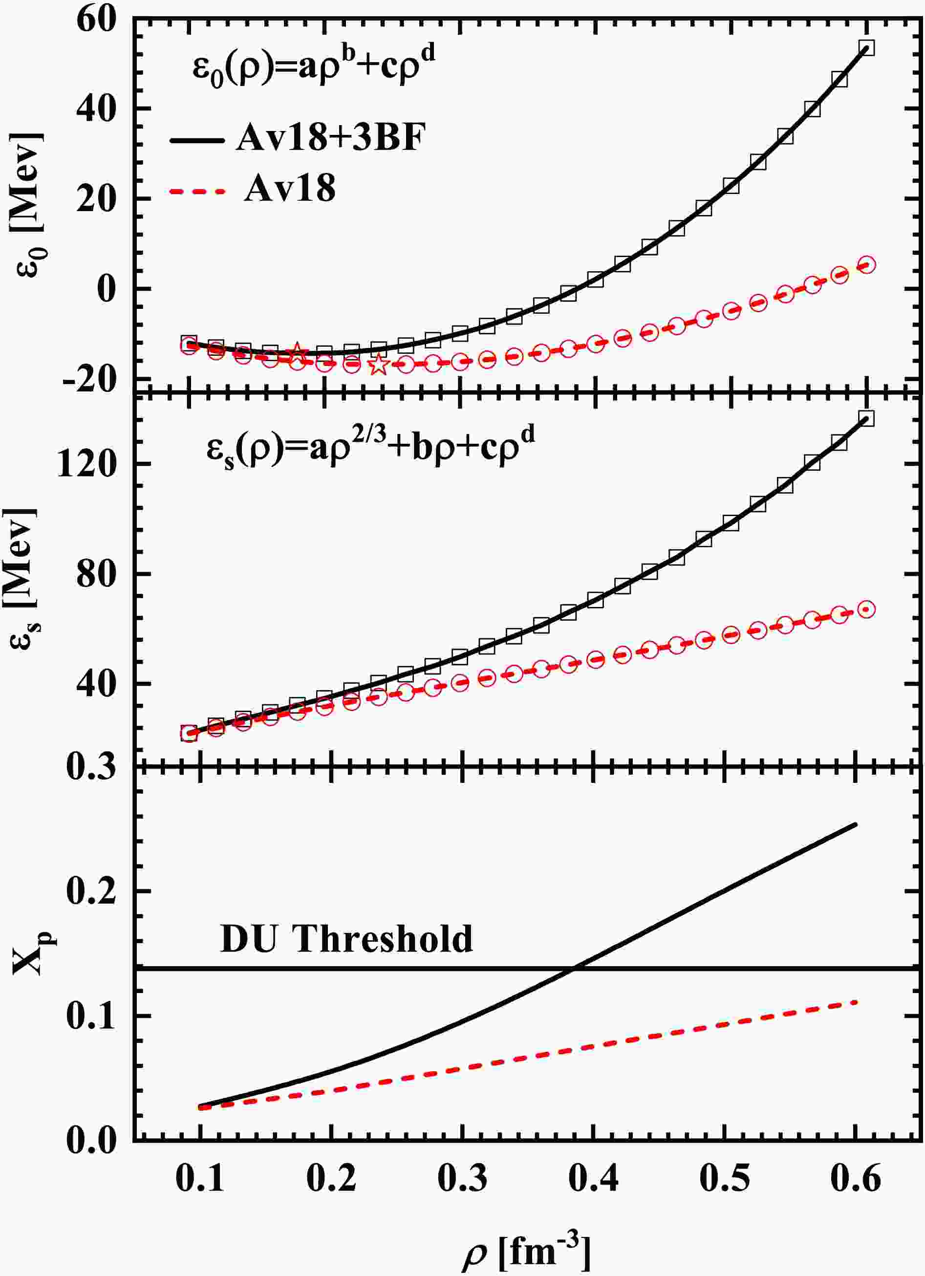
$ \varepsilon(\rho,\beta) $ . Owing to isospin symmetry,$ \varepsilon(\rho,\beta) $ can be characterized in terms of$ \varepsilon_0 $ and the symmetry energy$ \varepsilon_s $ . The results obtained within the BHF approach using the Av18 potential supplemented by a microscopic three-body force (3BF) [42−44] are shown in Fig. 1. For comparison, the results obtained with the Av18 potential alone are also displayed. Including the three-body force yields a saturation density of$ 0.186 {\rm{fm}}^{-3} $ and an energy per baryon at saturation of −14.5 MeV. It should be emphasized that these saturation properties include the contribution of the total momentum K. As noted in Ref. [49], an exact treatment of the total momentum substantially improves the saturation properties of symmetric nuclear matter (SNM). To evaluate the derivatives of$ \varepsilon_0 $ and$ \varepsilon_{s} $ with respect to ρ, we adopt the following forms: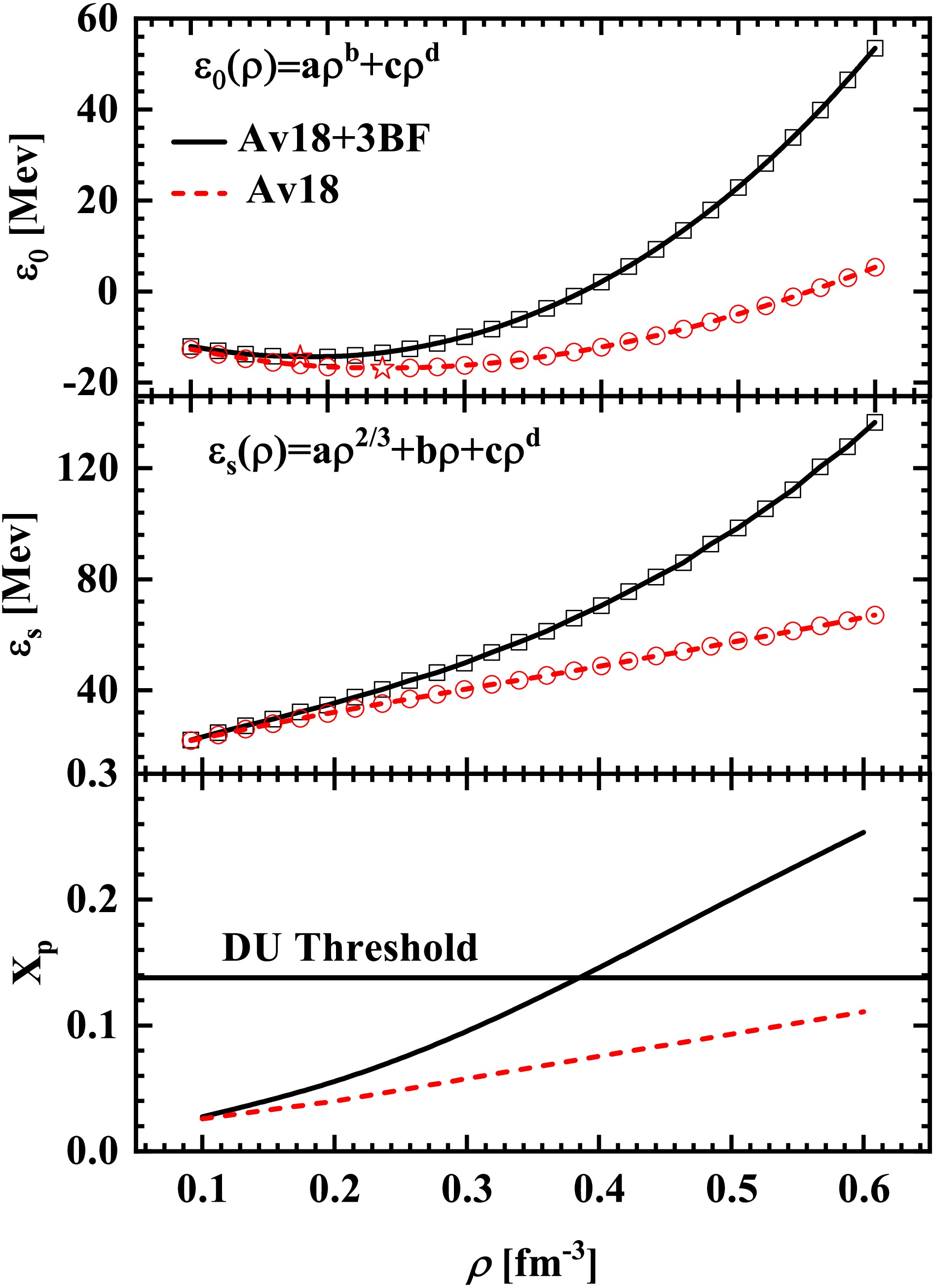
Figure 1. (color online) Binding energy per nucleon of symmetric nuclear matter
$ \varepsilon_0(\rho) $ (upper panel), nuclear symmetry energy$ \varepsilon_s $ (middle panel), and proton fraction of β–stable matter (lower panel) at zero temperature as functions of nucleon density. The black open squares and red open circles represent the results obtained with Av18 + 3BF and Av18 only, respectively. The black solid and red short-dashed lines in the upper and middle panels denote the corresponding fits obtained from Eq. (52). The red stars indicate the saturation points obtained from the BHF calculations. In the lower panel, the black solid and red short-dashed lines correspond to the results obtained with Av18 + 3BF and Av18 only, respectively. The horizontal line indicates the threshold proton fraction for the direct Urca (DU) neutrino emission process.$ \begin{split} \varepsilon_0(\rho)=a\rho^b+c\rho^d, \ \ \varepsilon_s(\rho)=a\rho^{\frac{2}{3}}+b\rho+c\rho^d , \end{split} $
(52) to fit their density dependence. The fitted parameters, together with the corresponding standard deviations, are presented in Table 1. For β–stable nuclear matter (BSM), the proton fraction is fixed by the conditions of β equilibrium and charge neutrality and, in practice, is determined by the symmetry energy
$ \varepsilon_s $ . This behavior is shown in the lower panel of Fig. 1. The horizontal line indicates the threshold proton fraction for the direct Urca (DU) neutrino-emission process. The inclusion of the three-body force stiffens the symmetry energy, which in turn increases the proton fraction, facilitates the onset of the DU process, and may lead to more rapid cooling in NSs [53].a b c d σ $ \varepsilon_{0}(\rho) $ with Av18+3BF−50.6542 0.592213 345.452 2.61383 0.018251 $ \varepsilon_{0}(\rho) $ with Av18−71.8258 0.694666 147.214 1.90246 0.020589 $ \varepsilon_{s}(\rho) $ with Av18+3BF142.048 −92.3655 361.866 2.70684 0.190923 $ \varepsilon_{s}(\rho) $ with Av18159.937 −145.965 98.3314 1.71881 0.068027 Table 1. Fitted functional parametrizations of the binding energy per nucleon in symmetric nuclear matter and of the nuclear symmetry energy as functions of nucleon density, together with their standard deviations.
For the effective mass, BHF results at various densities, isospin asymmetries, and temperatures, along with a parameterization, have been reported in [50]. We employ the same results here. The remaining key ingredient is the in-medium differential cross section, which plays a central role in determining transport properties. Figure 2 shows the differential neutron–neutron and neutron–proton cross sections in symmetric nuclear matter and β–stable nuclear matter. Because the differential cross section depends on the total momentum of the two scattering nucleons, we set the total momentum to
$ K=0 $ ; that is, the result is evaluated in the c.m. frame. For comparison, Fig. 2 also shows the free-space differential cross section and the result obtained from Eq. (38) using Av18 + 3BF with$ m^*/m=1 $ . The free-space differential cross section is in good agreement with the experimental data [54−56]. For symmetric nuclear matter, the results obtained with Av18 alone in the neutron–neutron channel agree with those of Refs. [9, 39]. When 3BF [43] is included, the trend remains similar, but the magnitude increases by roughly a factor of 1.6 because of differences in the three-body force. This difference is also reflected in the proton fraction. Neglecting medium effects on the scattering phase space (i.e., setting$ m^*/m=1 $ ) leads to a substantial increase in the cross section. This indicates that the medium modifies the nucleon–nucleon scattering cross section primarily by reducing the available scattering phase space. In β–stable nuclear matter, the neutron–neutron differential cross section exhibits essentially the same angular distribution as in symmetric nuclear matter, with only an overall change in magnitude. For the neutron–proton differential cross section, three-body forces are found to enhance the forward–backward scattering asymmetry. As in neutron–neutron scattering, neutron–proton scattering in β–stable nuclear matter exhibits behavior very similar to that in symmetric nuclear matter.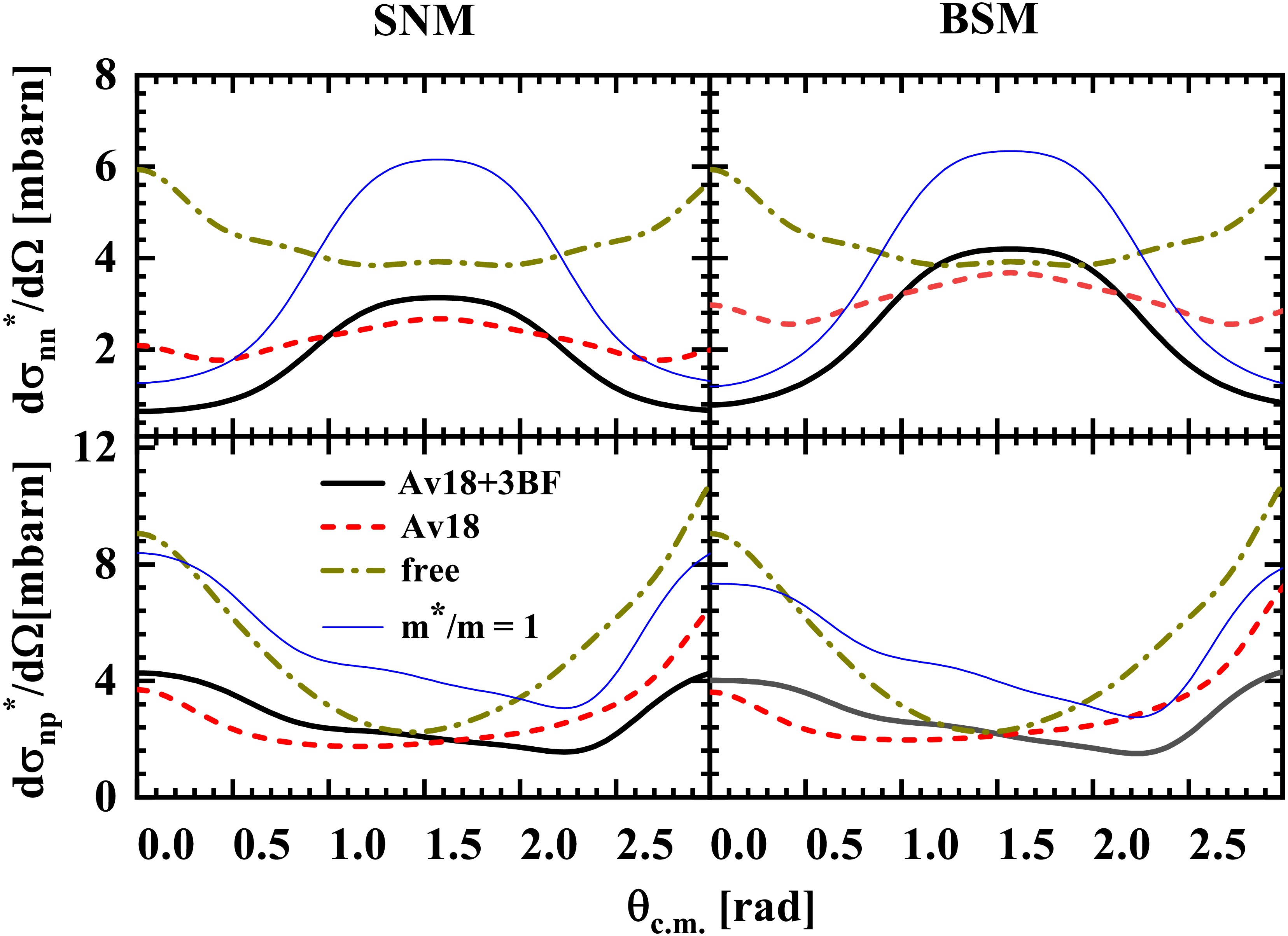
Figure 2. (color online) Differential cross sections as functions of the center-of-mass (c.m.) scattering angle at a density of
$ \rho=0.35\; {\rm{fm}}^{-3} $ and a c.m. energy of$ E_{{\rm{c.m.}}}=75\; {\rm{MeV}} $ . The left (right) panels correspond to symmetric nuclear matter (β–stable nuclear matter), whereas the upper (lower) panels show the neutron–neutron (neutron–proton) channel. The thick solid, thick short-dashed, and thick short-dash-dotted lines denote the results obtained with Av18 + 3BF, Av18 only, and in free space, respectively. The thin solid lines show the results calculated from Eq. (38) using Av18 + 3BF with$ m^{*}/m=1 $ .According to the approximate expression in Eq. (51), the isospin diffusion coefficient is inversely proportional to the effective total cross section
$ \sigma^{*} $ . To gain a qualitative understanding of the behavior of the total cross section, we show its density dependence in symmetric nuclear matter and in β–stable nuclear matter in Fig. 3. In symmetric nuclear matter, the effective neutron–proton cross section$ \sigma^{*}_{np} $ is much larger than the effective neutron– neutron and proton–proton cross sections,$ \sigma^{*}_{nn} $ and$ \sigma^{*}_{pp} $ , respectively. This indicates that the neutron–proton channel provides the dominant contribution to the diffusion coefficient. This conclusion also holds for β–stable nuclear matter with Av18+3BF. However, when only the Av18 two-body potential is adopted, the situation becomes unexpected: the effective proton–proton total cross section$ \sigma^{*}_{pp} $ becomes more pronounced than the neutron–neutron and neutron–proton total cross sections,$ \sigma^{*}_{nn} $ and$ \sigma^{*}_{np} $ . This behavior may be attributed to the fact that, when only the Av18 potential is considered, the cross section in the c.m. frame decreases monotonically with increasing incident momentum q (equivalently, the c.m. energy,$ E_{{\rm{c.m.}}}= \hbar^2q^2/m $ ). Meanwhile, the effective total cross section defined in Eq. (41) is dominated by contributions from the cross section evaluated at the Fermi surface. In β–stable matter, the proton Fermi momentum is much smaller than the neutron Fermi momentum, which makes the corresponding effective total cross section more pronounced. By contrast, when 3BF is included, the$ E_{{\rm{c.m.}}} $ (q) dependence of the cross section is no longer monotonic. However, when only the Av18 potential is taken into account for β–stable matter, the effective neutron–proton and proton–proton total cross sections,$ \sigma^{*}_{np} $ and$ \sigma^{*}_{pp} $ , are of comparable magnitude.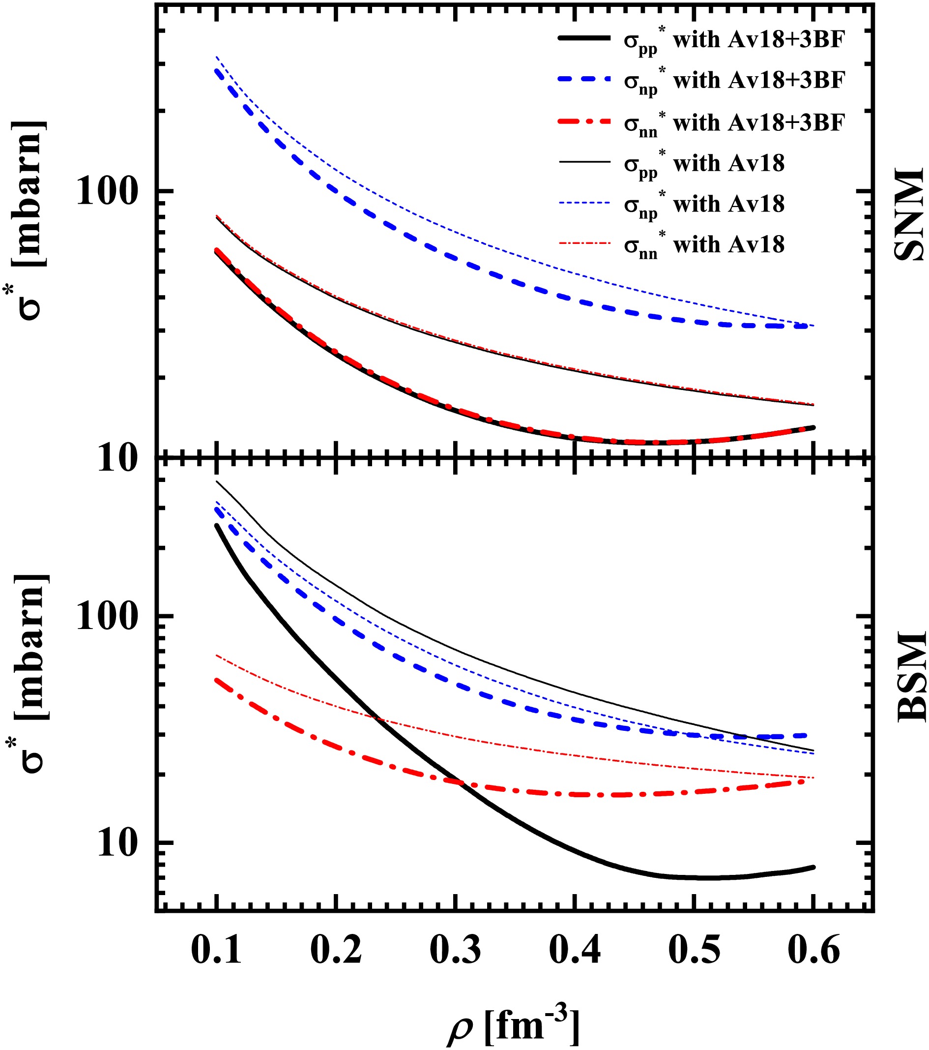
Figure 3. (color online) Effective total cross sections,
$ \sigma^* $ , as functions of density for symmetric nuclear matter (upper panel) and β–stable nuclear matter (lower panel). The black solid, blue short-dashed, and red short-dash-dotted lines denote the proton–proton and neutron–proton scattering results. The thick and thin lines indicate the results obtained with Av18 + 3BF and Av18 only, respectively.Based on the key input quantities discussed above, we present the isospin diffusion coefficients, with the temperature dependence factored out, for symmetric and β–stable nuclear matter, as shown in Fig. 4. The black solid lines denote the exact results obtained from Eq. (50). In general, the density dependence of the diffusion coefficient is inversely proportional to the effective total cross section
$ \sigma^* $ . The inclusion of three-body forces suppresses the nucleon–nucleon scattering cross sections, thereby enhancing the diffusion coefficient. To establish a more direct connection with the cross sections, we also show in Fig. 4 the results of the effective total cross section approximation (ETCSA), obtained from Eq. (51) and indicated by the red dashed lines. Given the importance of the neutron–proton cross section, as illustrated in Fig. 3, we further present the results of the neutron–proton cross section approximation (NPCSA), represented by the blue short-dashed lines. This approximation is obtained from Eq. (51) by retaining only the term$ \sigma^{*}_{np} $ and neglecting the contributions from$ \sigma^{*}_{nn} $ and$ \sigma^{*}_{pp} $ . For comparison, we also show the results of the total cross section approximation (TCSA), denoted by the dash-dotted lines in Fig. 4. In this case, Eq. (51) is evaluated with$ \sigma^* $ replaced by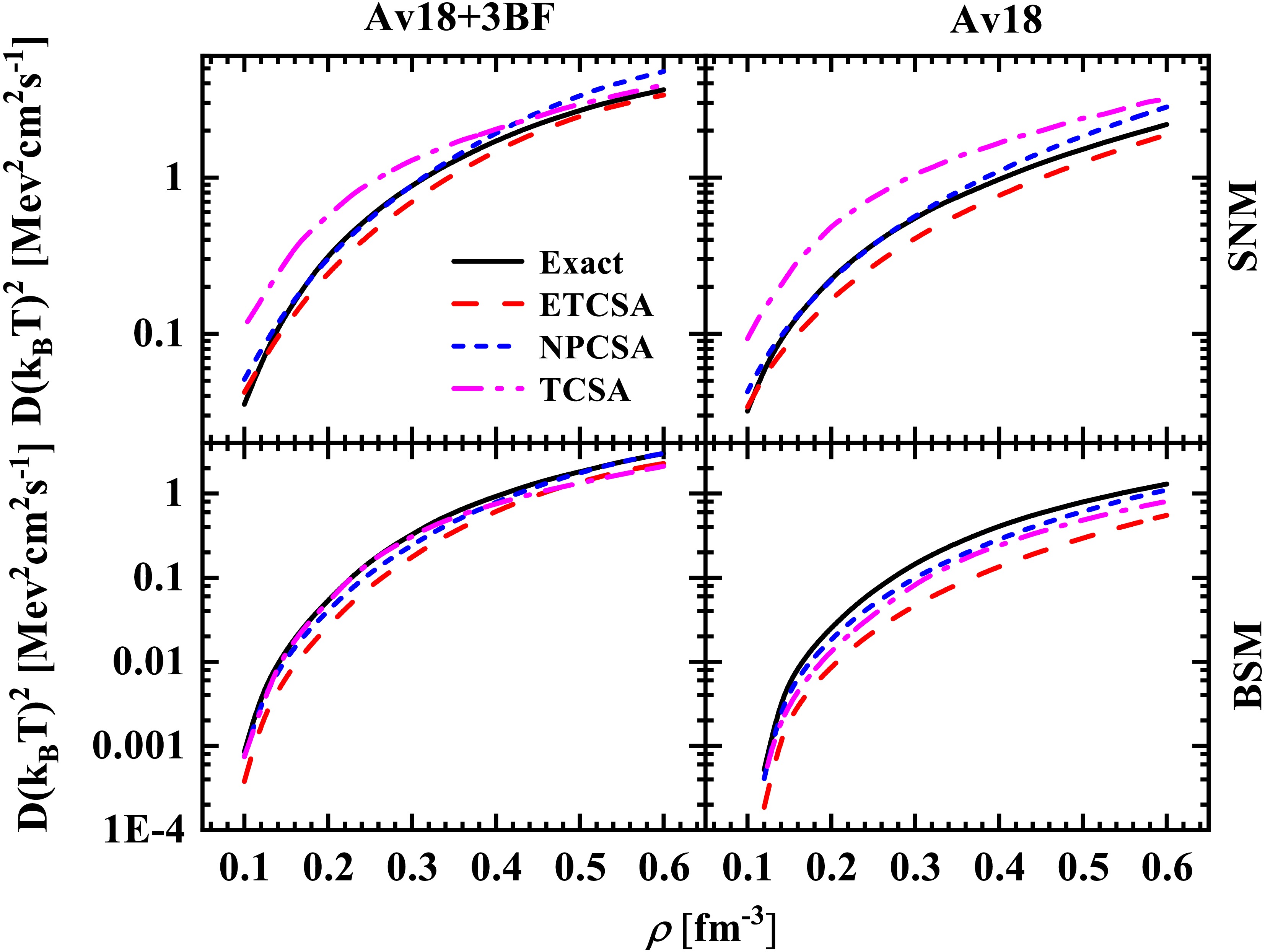
Figure 4. (color online) Isospin diffusion coefficients obtained under different approximations in symmetric and β–stable nuclear matter. The black solid, red dashed, blue short-dashed, and magenta dash-dotted lines denote the exact result, the effective total cross-section approximation (ETCSA), the neutron–proton cross-section approximation (NPCSA), and the total cross-section approximation (TCSA), respectively.
$ \begin{split}\sigma_{\tau\tau'}^F = \frac{1}{1+\delta_{\tau\tau'}}\int_{(4\pi)}^{ }\mathrm{d}\Omega_{\rm{c.m.}}\frac{\mathrm{d}\sigma_{\tau\tau'}^*}{\mathrm{d}\Omega_{\rm{c.m.}}}(K,q,\theta_{\rm{c.m.}}),\end{split} $
(53) where
$ K=0 $ and$ q=|p_\tau-p_{\tau'}|/(2\hbar) $ in the c.m. frame. The quantity$ \sigma^F_{\tau\tau'} $ corresponds to the total cross section evaluated at the c.m. energy$ E_{{\rm{c.m.}}}=\hbar^2q^2/m $ . Overall, although these approximations reproduce the order of magnitude and the general density dependence of the exact results, substantial quantitative deviations remain. In particular, within ETCSA, the diffusion coefficients for SNM with Av18+3BF, SNM with Av18, BSM with Av18+3BF, and BSM with Av18 exceed the corresponding exact results by factors of approximately 1.12, 1.21, 1.38, and 2.54, respectively. For TCSA, the corresponding ratios are approximately 0.85, 0.62, 1.34, and 1.63, respectively. Part of the discrepancy between the approximations and the exact results arises because the approximate formula (51) does not incorporate the correction factor$ C_{\lambda_n} $ that appears in the AK theory. Given the strong density dependence of$ C_{\lambda_n} $ , its magnitude varies substantially in β–stable nuclear matter, ranging from 1.4 to 2.2 with 3BF, and from 2.0 to 2.7 without 3BF. Consequently, the deviations of the ETCSA and TCSA results from the exact solution cannot be eliminated by introducing a simple universal renormalization factor. However, it is worth emphasizing that NPCSA provides a relatively better approximation and exhibits a certain degree of universality. Regardless of whether three-body forces are included, the approximate diffusion coefficients deviate from the corresponding exact results by factors of roughly 0.82 and 1.2 for SNM and BSM, respectively. This seemingly surprising success of NPCSA may originate from the underlying mechanism of isospin diffusion. Physically, isospin diffusion is governed by relative transport between neutrons and protons. Although nn and pp collisions primarily redistribute momentum within each species, they do not directly change the isospin composition. In contrast, np scattering directly modifies the distributions of the two components and thus dominates the equilibration of isospin asymmetry. As a result, retaining only the np channel already captures the leading mechanism of the diffusion process, explaining why the approximation works well. This feature is expected to be largely independent of the specific interaction used.Notably, in BSM with Av18 alone, the proton–proton cross section
$ \sigma^*_{pp} $ is slightly larger than the neutron–proton cross section$ \sigma^*_{np} $ . Consequently, for the proton diffusion coefficient$ \tilde{D}_p $ , the two channels make approximately comparable contributions, each accounting for roughly one half. Moreover, owing to the presence of the$ (1+\beta)^2 $ factor in the expression for$ \tilde{D}_p $ [in contrast to$ (1-\beta)^2 $ for$ \tilde{D}_n $ ], the proton component becomes much more significant in the total diffusion coefficient. As a result, the$ \sigma^*_{pp} $ channel contributes about one half of the total D. However, the AK correction factor$ C_{\lambda_n} $ takes values in the range$ 2 $ –$ 2.7 $ , which largely compensates for the deviation introduced by adopting only$ \sigma^*_{np} $ . Nevertheless, for BSM with Av18 alone, the corresponding NPCSA results still deviate slightly more from the exact values than the NPCSA results in the other cases.Experimentally measured isospin diffusion observables in heavy-ion collisions have been widely used to constrain the density dependence of the symmetry energy [3, 7, 57]. In this context, it is useful to clarify the connection between the microscopic diffusion coefficient calculated in uniform nuclear matter and experimentally accessible observables, such as the isospin transport ratio
$ R_{i} $ [57]. In transport simulations [e.g., Boltzmann–Uehling–Uhlenbeck (BUU) or Quantum Molecular Dynamics (QMD) transport models], the equilibration of the neutron–proton asymmetry arises dynamically from the combined effects of mean fields and nucleon–nucleon collisions. Although these models do not explicitly introduce a diffusion coefficient, the underlying transport process can be approximated, in the linear response regime near local equilibrium, by a diffusion equation for the isospin asymmetry. In this limit, the diffusion coefficient D may provide an effective characterization of local transport properties, reflecting both the symmetry energy and in-medium scattering cross sections. Thus, although D is not directly measurable, it can serve as a useful intermediate quantity that connects microscopic transport properties to the dynamics underlying macroscopic observables, such as$ R_{i} $ , which are used to constrain the symmetry energy.A reliable interpretation of such observables may require a clear understanding of the isospin dependence of the diffusion coefficient in nuclear matter. We therefore show the isospin dependence of the diffusion coefficient as a function of the isospin asymmetry β in Fig. 5. In general, the β dependence of the diffusion coefficient deviates significantly from the simple
$ (1-\beta^2) $ parameterization adopted in Ref. [13]. Instead, it exhibits a more intricate functional behavior characterized by a symmetric double-peaked structure ("M"-shaped structure). Specifically, once the system departs from symmetric nuclear matter, the diffusion coefficient initially increases with increasing β, reaches a maximum at a certain value of β, and then decreases at larger asymmetries. For the Av18+3BF calculations, the peaks are located at$ |\beta| \approx 0.2 $ and$ |\beta| \approx 0.26 $ for densities$ \rho=0.17\; {\rm{fm}}^{-3} $ and$ 0.34\; {\rm{fm}}^{-3} $ , respectively. In contrast, for the calculation with the Av18 interaction alone, the corresponding maxima appear at$ |\beta| \approx 0.12 $ and$ |\beta| \approx 0.31 $ . The β dependence of D arises from four factors:$ \chi_{{\cal{P}}} $ ,$ p_{\tau}^{3}(\varsigma_\tau-\beta)^2 $ ,$ m^{*}_\tau $ , and$ \overline{\nu}_\tau $ . Although the β dependence of$ \chi_{{\cal{P}}} $ is explicitly given by Eq. (31), the other three contributions are intertwined. To analyze the β dependence of the isospin diffusion coefficient more clearly, we also present the β dependence of$ D\chi_{{\cal{P}}} $ in Fig. 5. The β dependence of$ D\chi_{{\cal{P}}} $ displays a pronounced double-peaked structure. The locations of the peaks are nearly independent of the density and the interaction, remaining around$ |\beta|=0.35 $ . These results indicate that the symmetric double-peaked structure of the diffusion coefficient originates from$ D\chi_{{\cal{P}}} $ and that the locations of the peaks may be determined by the susceptibility$ \chi_{{\cal{P}}} $ . To quantify the β dependence of$ D\chi_{{\cal{P}}} $ , we further fit$ D\chi_{{\cal{P}}} $ with the following functional form: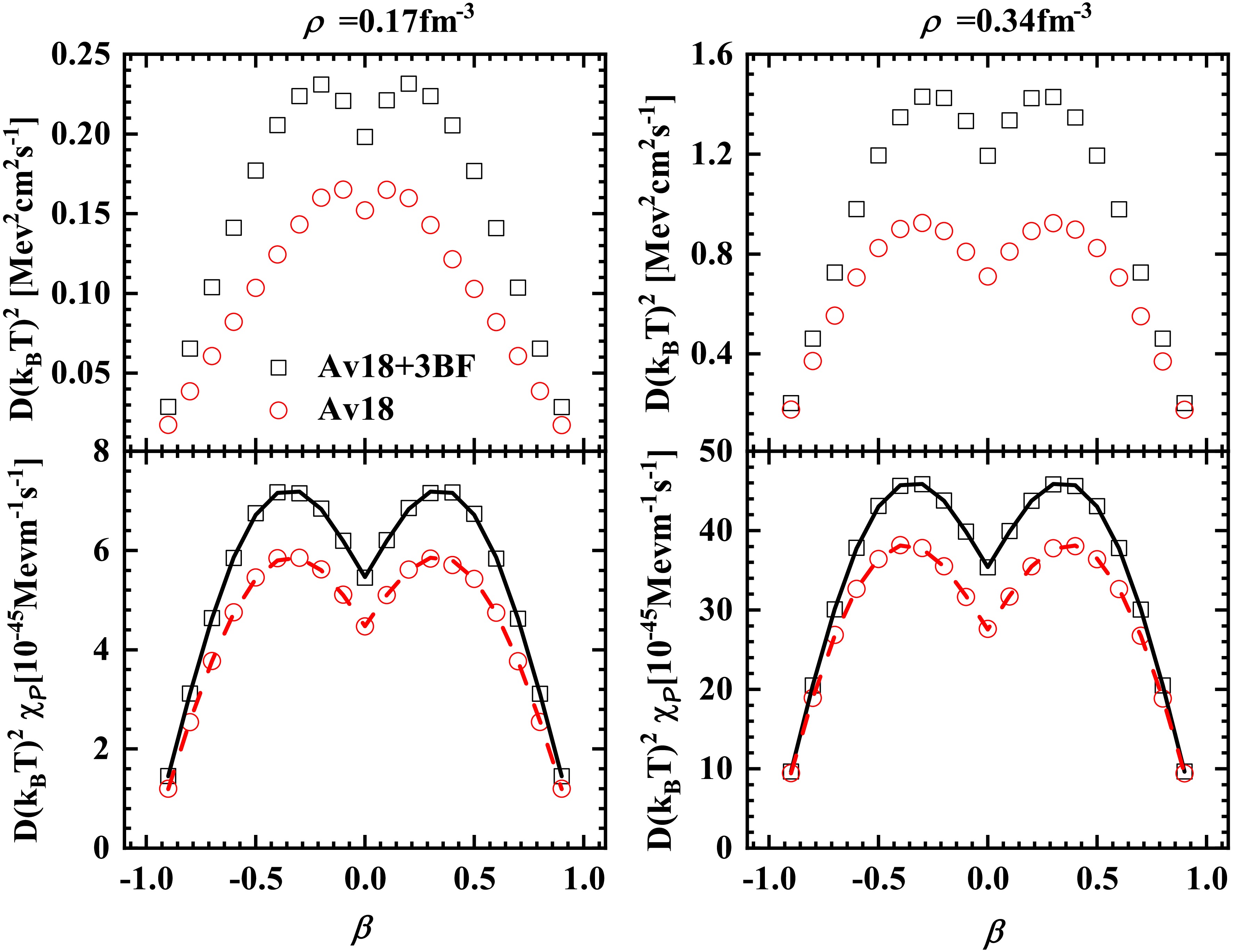
Figure 5. (color online) Isospin dependence of the diffusion coefficient D (upper panel) and
$ D\chi_{{\cal{P}}} $ (lower panel) at densities of$ 0.17\;{\rm{fm}}^{-3} $ and$ 0.34\;{\rm{fm}}^{-3} $ . The black open squares and red open circles represent the results obtained using Av18 + 3BF and Av18 alone, respectively. The black solid and red short-dashed lines in the lower panel denote the corresponding fits obtained from Eq. (54).$ \begin{split} D\chi_{{\cal{P}}}=&a+b\sqrt{\eta+\beta^2}+c\Bigg(\sqrt{\eta+\beta^2}\Bigg)^2+d\Bigg(\sqrt{\eta+\beta^2}\Bigg)^3\\&+e\Bigg(\sqrt{\eta+\beta^2}\Bigg)^4. \end{split} $
(54) The fitted parameters, together with their corresponding standard deviations, are presented in Table 2. The parameter η is introduced as a small regulator to ensure continuity at
$ \beta=0 $ . Although the linear dependence of$ D\chi_{{\cal{P}}} $ on β is numerically important, isospin symmetry requires$ D\chi_{{\cal{P}}} $ to be an even function of β. In practical applications, we adopt$ \eta=0.01^2 $ . We note that the dominance of the coefficient multiplying the term$ \sqrt{\eta+\beta^2} $ , relative to that multiplying the term$ \eta+\beta^2 $ , leads to an approximately symmetric, quasi-linear dependence of$ D\chi_{{\cal{P}}} $ on β at small isospin asymmetry. In practice, for$ |\beta|<0.15 $ ,$ D\chi_{{\cal{P}}} $ is well approximated by the form$ a+b|\beta| $ .a b c d e σ $ \rho=0.17 $ with Av18+3BF5.378 8.406 0.0554 −31.976 17.945 0.0163 $ \rho=0.17 $ with Av184.400 7.660 −5.252 −16.806 9.760 0.0262 $ \rho=0.34 $ with Av18+3BF34.895 51.844 −6.114 −177.896 95.601 0.0508 $ \rho=0.34 $ with Av1827.049 49.802 −17.498 −117.045 56.502 0.0596 Table 2. Fitted parameters and standard deviations of the functions for the diffusion coefficient multiplied by the generalized susceptibility, i.e.,
$ D\chi_{{\cal{P}}} $ .Although the diffusion coefficient obtained in the present work is, in principle, restricted to the low-temperature limit, the isospin dependence (the ''M''-shaped structure) derived here is expected to remain relevant for studies of isospin diffusion. In typical heavy-ion collision scenarios for isospin-diffusion studies [2, 3, 6, 7], the corresponding effective temperatures are on the order of 5 MeV and thus remain relatively low compared with the Fermi energy of nuclear matter. As a result, key input quantities, such as the susceptibility, effective mass, and in-medium differential cross section, are not expected to differ significantly from their zero-temperature values. More importantly, their isospin dependence is expected to remain largely unchanged as temperature increases. Therefore, the β dependence of the diffusion coefficient obtained in the present work is expected to be robust in applications to isospin-diffusion studies.
-
The evaluation of the isospin diffusion coefficient in nuclear matter requires several key inputs, including the susceptibility, effective mass, and transition probability (or, equivalently, the differential cross section), all of which are calculated self-consistently within the BHF approach. The formalism was introduced in the theoretical section. Below, we present the corresponding results.
In the low-temperature limit, the susceptibility of nuclear matter is determined primarily by the single-particle binding energy
$ \varepsilon(\rho,\beta) $ . Owing to isospin symmetry,$ \varepsilon(\rho,\beta) $ can be characterized in terms of$ \varepsilon_0 $ and the symmetry energy$ \varepsilon_s $ . The results obtained within the BHF approach using the Av18 potential supplemented by a microscopic three-body force (3BF) [42−44] are shown in Fig. 1. For comparison, the results obtained with the Av18 potential alone are also displayed. Including the three-body force yields a saturation density of$ 0.186 {\rm{fm}}^{-3} $ and an energy per baryon at saturation of −14.5 MeV. It should be emphasized that these saturation properties include the contribution of the total momentum K. As noted in Ref. [49], an exact treatment of the total momentum substantially improves the saturation properties of symmetric nuclear matter (SNM). To evaluate the derivatives of$ \varepsilon_0 $ and$ \varepsilon_{s} $ with respect to ρ, we adopt the following forms:
Figure 1. (color online) Binding energy per nucleon of symmetric nuclear matter
$ \varepsilon_0(\rho) $ (upper panel), nuclear symmetry energy$ \varepsilon_s $ (middle panel), and proton fraction of β–stable matter (lower panel) at zero temperature as functions of nucleon density. The black open squares and red open circles represent the results obtained with Av18 + 3BF and Av18 only, respectively. The black solid and red short-dashed lines in the upper and middle panels denote the corresponding fits obtained from Eq. (52). The red stars indicate the saturation points obtained from the BHF calculations. In the lower panel, the black solid and red short-dashed lines correspond to the results obtained with Av18 + 3BF and Av18 only, respectively. The horizontal line indicates the threshold proton fraction for the direct Urca (DU) neutrino emission process.$ \begin{split} \varepsilon_0(\rho)=a\rho^b+c\rho^d, \ \ \varepsilon_s(\rho)=a\rho^{\frac{2}{3}}+b\rho+c\rho^d , \end{split} $
(52) to fit their density dependence. The fitted parameters, together with the corresponding standard deviations, are presented in Table 1. For β–stable nuclear matter (BSM), the proton fraction is fixed by the conditions of β equilibrium and charge neutrality and, in practice, is determined by the symmetry energy
$ \varepsilon_s $ . This behavior is shown in the lower panel of Fig. 1. The horizontal line indicates the threshold proton fraction for the direct Urca (DU) neutrino-emission process. The inclusion of the three-body force stiffens the symmetry energy, which in turn increases the proton fraction, facilitates the onset of the DU process, and may lead to more rapid cooling in NSs [53].a b c d σ $ \varepsilon_{0}(\rho) $ with Av18+3BF−50.6542 0.592213 345.452 2.61383 0.018251 $ \varepsilon_{0}(\rho) $ with Av18−71.8258 0.694666 147.214 1.90246 0.020589 $ \varepsilon_{s}(\rho) $ with Av18+3BF142.048 −92.3655 361.866 2.70684 0.190923 $ \varepsilon_{s}(\rho) $ with Av18159.937 −145.965 98.3314 1.71881 0.068027 Table 1. Fitted functional parametrizations of the binding energy per nucleon in symmetric nuclear matter and of the nuclear symmetry energy as functions of nucleon density, together with their standard deviations.
For the effective mass, BHF results at various densities, isospin asymmetries, and temperatures, along with a parameterization, have been reported in [50]. We employ the same results here. The remaining key ingredient is the in-medium differential cross section, which plays a central role in determining transport properties. Figure 2 shows the differential neutron–neutron and neutron–proton cross sections in symmetric nuclear matter and β–stable nuclear matter. Because the differential cross section depends on the total momentum of the two scattering nucleons, we set the total momentum to
$ K=0 $ ; that is, the result is evaluated in the c.m. frame. For comparison, Fig. 2 also shows the free-space differential cross section and the result obtained from Eq. (38) using Av18 + 3BF with$ m^*/m=1 $ . The free-space differential cross section is in good agreement with the experimental data [54−56]. For symmetric nuclear matter, the results obtained with Av18 alone in the neutron–neutron channel agree with those of Refs. [9, 39]. When 3BF [43] is included, the trend remains similar, but the magnitude increases by roughly a factor of 1.6 because of differences in the three-body force. This difference is also reflected in the proton fraction. Neglecting medium effects on the scattering phase space (i.e., setting$ m^*/m=1 $ ) leads to a substantial increase in the cross section. This indicates that the medium modifies the nucleon–nucleon scattering cross section primarily by reducing the available scattering phase space. In β–stable nuclear matter, the neutron–neutron differential cross section exhibits essentially the same angular distribution as in symmetric nuclear matter, with only an overall change in magnitude. For the neutron–proton differential cross section, three-body forces are found to enhance the forward–backward scattering asymmetry. As in neutron–neutron scattering, neutron–proton scattering in β–stable nuclear matter exhibits behavior very similar to that in symmetric nuclear matter.
Figure 2. (color online) Differential cross sections as functions of the center-of-mass (c.m.) scattering angle at a density of
$ \rho=0.35\; {\rm{fm}}^{-3} $ and a c.m. energy of$ E_{{\rm{c.m.}}}=75\; {\rm{MeV}} $ . The left (right) panels correspond to symmetric nuclear matter (β–stable nuclear matter), whereas the upper (lower) panels show the neutron–neutron (neutron–proton) channel. The thick solid, thick short-dashed, and thick short-dash-dotted lines denote the results obtained with Av18 + 3BF, Av18 only, and in free space, respectively. The thin solid lines show the results calculated from Eq. (38) using Av18 + 3BF with$ m^{*}/m=1 $ .According to the approximate expression in Eq. (51), the isospin diffusion coefficient is inversely proportional to the effective total cross section
$ \sigma^{*} $ . To gain a qualitative understanding of the behavior of the total cross section, we show its density dependence in symmetric nuclear matter and in β–stable nuclear matter in Fig. 3. In symmetric nuclear matter, the effective neutron–proton cross section$ \sigma^{*}_{np} $ is much larger than the effective neutron– neutron and proton–proton cross sections,$ \sigma^{*}_{nn} $ and$ \sigma^{*}_{pp} $ , respectively. This indicates that the neutron–proton channel provides the dominant contribution to the diffusion coefficient. This conclusion also holds for β–stable nuclear matter with Av18+3BF. However, when only the Av18 two-body potential is adopted, the situation becomes unexpected: the effective proton–proton total cross section$ \sigma^{*}_{pp} $ becomes more pronounced than the neutron–neutron and neutron–proton total cross sections,$ \sigma^{*}_{nn} $ and$ \sigma^{*}_{np} $ . This behavior may be attributed to the fact that, when only the Av18 potential is considered, the cross section in the c.m. frame decreases monotonically with increasing incident momentum q (equivalently, the c.m. energy,$ E_{{\rm{c.m.}}}= \hbar^2q^2/m $ ). Meanwhile, the effective total cross section defined in Eq. (41) is dominated by contributions from the cross section evaluated at the Fermi surface. In β–stable matter, the proton Fermi momentum is much smaller than the neutron Fermi momentum, which makes the corresponding effective total cross section more pronounced. By contrast, when 3BF is included, the$ E_{{\rm{c.m.}}} $ (q) dependence of the cross section is no longer monotonic. However, when only the Av18 potential is taken into account for β–stable matter, the effective neutron–proton and proton–proton total cross sections,$ \sigma^{*}_{np} $ and$ \sigma^{*}_{pp} $ , are of comparable magnitude.
Figure 3. (color online) Effective total cross sections,
$ \sigma^* $ , as functions of density for symmetric nuclear matter (upper panel) and β–stable nuclear matter (lower panel). The black solid, blue short-dashed, and red short-dash-dotted lines denote the proton–proton and neutron–proton scattering results. The thick and thin lines indicate the results obtained with Av18 + 3BF and Av18 only, respectively.Based on the key input quantities discussed above, we present the isospin diffusion coefficients, with the temperature dependence factored out, for symmetric and β–stable nuclear matter, as shown in Fig. 4. The black solid lines denote the exact results obtained from Eq. (50). In general, the density dependence of the diffusion coefficient is inversely proportional to the effective total cross section
$ \sigma^* $ . The inclusion of three-body forces suppresses the nucleon–nucleon scattering cross sections, thereby enhancing the diffusion coefficient. To establish a more direct connection with the cross sections, we also show in Fig. 4 the results of the effective total cross section approximation (ETCSA), obtained from Eq. (51) and indicated by the red dashed lines. Given the importance of the neutron–proton cross section, as illustrated in Fig. 3, we further present the results of the neutron–proton cross section approximation (NPCSA), represented by the blue short-dashed lines. This approximation is obtained from Eq. (51) by retaining only the term$ \sigma^{*}_{np} $ and neglecting the contributions from$ \sigma^{*}_{nn} $ and$ \sigma^{*}_{pp} $ . For comparison, we also show the results of the total cross section approximation (TCSA), denoted by the dash-dotted lines in Fig. 4. In this case, Eq. (51) is evaluated with$ \sigma^* $ replaced by
Figure 4. (color online) Isospin diffusion coefficients obtained under different approximations in symmetric and β–stable nuclear matter. The black solid, red dashed, blue short-dashed, and magenta dash-dotted lines denote the exact result, the effective total cross-section approximation (ETCSA), the neutron–proton cross-section approximation (NPCSA), and the total cross-section approximation (TCSA), respectively.
$ \begin{split}\sigma_{\tau\tau'}^F = \frac{1}{1+\delta_{\tau\tau'}}\int_{(4\pi)}^{ }\mathrm{d}\Omega_{\rm{c.m.}}\frac{\mathrm{d}\sigma_{\tau\tau'}^*}{\mathrm{d}\Omega_{\rm{c.m.}}}(K,q,\theta_{\rm{c.m.}}),\end{split} $
(53) where
$ K=0 $ and$ q=|p_\tau-p_{\tau'}|/(2\hbar) $ in the c.m. frame. The quantity$ \sigma^F_{\tau\tau'} $ corresponds to the total cross section evaluated at the c.m. energy$ E_{{\rm{c.m.}}}=\hbar^2q^2/m $ . Overall, although these approximations reproduce the order of magnitude and the general density dependence of the exact results, substantial quantitative deviations remain. In particular, within ETCSA, the diffusion coefficients for SNM with Av18+3BF, SNM with Av18, BSM with Av18+3BF, and BSM with Av18 exceed the corresponding exact results by factors of approximately 1.12, 1.21, 1.38, and 2.54, respectively. For TCSA, the corresponding ratios are approximately 0.85, 0.62, 1.34, and 1.63, respectively. Part of the discrepancy between the approximations and the exact results arises because the approximate formula (51) does not incorporate the correction factor$ C_{\lambda_n} $ that appears in the AK theory. Given the strong density dependence of$ C_{\lambda_n} $ , its magnitude varies substantially in β–stable nuclear matter, ranging from 1.4 to 2.2 with 3BF, and from 2.0 to 2.7 without 3BF. Consequently, the deviations of the ETCSA and TCSA results from the exact solution cannot be eliminated by introducing a simple universal renormalization factor. However, it is worth emphasizing that NPCSA provides a relatively better approximation and exhibits a certain degree of universality. Regardless of whether three-body forces are included, the approximate diffusion coefficients deviate from the corresponding exact results by factors of roughly 0.82 and 1.2 for SNM and BSM, respectively. This seemingly surprising success of NPCSA may originate from the underlying mechanism of isospin diffusion. Physically, isospin diffusion is governed by relative transport between neutrons and protons. Although nn and pp collisions primarily redistribute momentum within each species, they do not directly change the isospin composition. In contrast, np scattering directly modifies the distributions of the two components and thus dominates the equilibration of isospin asymmetry. As a result, retaining only the np channel already captures the leading mechanism of the diffusion process, explaining why the approximation works well. This feature is expected to be largely independent of the specific interaction used.Notably, in BSM with Av18 alone, the proton–proton cross section
$ \sigma^*_{pp} $ is slightly larger than the neutron–proton cross section$ \sigma^*_{np} $ . Consequently, for the proton diffusion coefficient$ \tilde{D}_p $ , the two channels make approximately comparable contributions, each accounting for roughly one half. Moreover, owing to the presence of the$ (1+\beta)^2 $ factor in the expression for$ \tilde{D}_p $ [in contrast to$ (1-\beta)^2 $ for$ \tilde{D}_n $ ], the proton component becomes much more significant in the total diffusion coefficient. As a result, the$ \sigma^*_{pp} $ channel contributes about one half of the total D. However, the AK correction factor$ C_{\lambda_n} $ takes values in the range$ 2 $ –$ 2.7 $ , which largely compensates for the deviation introduced by adopting only$ \sigma^*_{np} $ . Nevertheless, for BSM with Av18 alone, the corresponding NPCSA results still deviate slightly more from the exact values than the NPCSA results in the other cases.Experimentally measured isospin diffusion observables in heavy-ion collisions have been widely used to constrain the density dependence of the symmetry energy [3, 7, 57]. In this context, it is useful to clarify the connection between the microscopic diffusion coefficient calculated in uniform nuclear matter and experimentally accessible observables, such as the isospin transport ratio
$ R_{i} $ [57]. In transport simulations [e.g., Boltzmann–Uehling–Uhlenbeck (BUU) or Quantum Molecular Dynamics (QMD) transport models], the equilibration of the neutron–proton asymmetry arises dynamically from the combined effects of mean fields and nucleon–nucleon collisions. Although these models do not explicitly introduce a diffusion coefficient, the underlying transport process can be approximated, in the linear response regime near local equilibrium, by a diffusion equation for the isospin asymmetry. In this limit, the diffusion coefficient D may provide an effective characterization of local transport properties, reflecting both the symmetry energy and in-medium scattering cross sections. Thus, although D is not directly measurable, it can serve as a useful intermediate quantity that connects microscopic transport properties to the dynamics underlying macroscopic observables, such as$ R_{i} $ , which are used to constrain the symmetry energy.A reliable interpretation of such observables may require a clear understanding of the isospin dependence of the diffusion coefficient in nuclear matter. We therefore show the isospin dependence of the diffusion coefficient as a function of the isospin asymmetry β in Fig. 5. In general, the β dependence of the diffusion coefficient deviates significantly from the simple
$ (1-\beta^2) $ parameterization adopted in Ref. [13]. Instead, it exhibits a more intricate functional behavior characterized by a symmetric double-peaked structure ("M"-shaped structure). Specifically, once the system departs from symmetric nuclear matter, the diffusion coefficient initially increases with increasing β, reaches a maximum at a certain value of β, and then decreases at larger asymmetries. For the Av18+3BF calculations, the peaks are located at$ |\beta| \approx 0.2 $ and$ |\beta| \approx 0.26 $ for densities$ \rho=0.17\; {\rm{fm}}^{-3} $ and$ 0.34\; {\rm{fm}}^{-3} $ , respectively. In contrast, for the calculation with the Av18 interaction alone, the corresponding maxima appear at$ |\beta| \approx 0.12 $ and$ |\beta| \approx 0.31 $ . The β dependence of D arises from four factors:$ \chi_{{\cal{P}}} $ ,$ p_{\tau}^{3}(\varsigma_\tau-\beta)^2 $ ,$ m^{*}_\tau $ , and$ \overline{\nu}_\tau $ . Although the β dependence of$ \chi_{{\cal{P}}} $ is explicitly given by Eq. (31), the other three contributions are intertwined. To analyze the β dependence of the isospin diffusion coefficient more clearly, we also present the β dependence of$ D\chi_{{\cal{P}}} $ in Fig. 5. The β dependence of$ D\chi_{{\cal{P}}} $ displays a pronounced double-peaked structure. The locations of the peaks are nearly independent of the density and the interaction, remaining around$ |\beta|=0.35 $ . These results indicate that the symmetric double-peaked structure of the diffusion coefficient originates from$ D\chi_{{\cal{P}}} $ and that the locations of the peaks may be determined by the susceptibility$ \chi_{{\cal{P}}} $ . To quantify the β dependence of$ D\chi_{{\cal{P}}} $ , we further fit$ D\chi_{{\cal{P}}} $ with the following functional form:
Figure 5. (color online) Isospin dependence of the diffusion coefficient D (upper panel) and
$ D\chi_{{\cal{P}}} $ (lower panel) at densities of$ 0.17\;{\rm{fm}}^{-3} $ and$ 0.34\;{\rm{fm}}^{-3} $ . The black open squares and red open circles represent the results obtained using Av18 + 3BF and Av18 alone, respectively. The black solid and red short-dashed lines in the lower panel denote the corresponding fits obtained from Eq. (54).$ \begin{split} D\chi_{{\cal{P}}}=&a+b\sqrt{\eta+\beta^2}+c\Bigg(\sqrt{\eta+\beta^2}\Bigg)^2+d\Bigg(\sqrt{\eta+\beta^2}\Bigg)^3\\&+e\Bigg(\sqrt{\eta+\beta^2}\Bigg)^4. \end{split} $
(54) The fitted parameters, together with their corresponding standard deviations, are presented in Table 2. The parameter η is introduced as a small regulator to ensure continuity at
$ \beta=0 $ . Although the linear dependence of$ D\chi_{{\cal{P}}} $ on β is numerically important, isospin symmetry requires$ D\chi_{{\cal{P}}} $ to be an even function of β. In practical applications, we adopt$ \eta=0.01^2 $ . We note that the dominance of the coefficient multiplying the term$ \sqrt{\eta+\beta^2} $ , relative to that multiplying the term$ \eta+\beta^2 $ , leads to an approximately symmetric, quasi-linear dependence of$ D\chi_{{\cal{P}}} $ on β at small isospin asymmetry. In practice, for$ |\beta|<0.15 $ ,$ D\chi_{{\cal{P}}} $ is well approximated by the form$ a+b|\beta| $ .a b c d e σ $ \rho=0.17 $ with Av18+3BF5.378 8.406 0.0554 −31.976 17.945 0.0163 $ \rho=0.17 $ with Av184.400 7.660 −5.252 −16.806 9.760 0.0262 $ \rho=0.34 $ with Av18+3BF34.895 51.844 −6.114 −177.896 95.601 0.0508 $ \rho=0.34 $ with Av1827.049 49.802 −17.498 −117.045 56.502 0.0596 Table 2. Fitted parameters and standard deviations of the functions for the diffusion coefficient multiplied by the generalized susceptibility, i.e.,
$ D\chi_{{\cal{P}}} $ .Although the diffusion coefficient obtained in the present work is, in principle, restricted to the low-temperature limit, the isospin dependence (the ''M''-shaped structure) derived here is expected to remain relevant for studies of isospin diffusion. In typical heavy-ion collision scenarios for isospin-diffusion studies [2, 3, 6, 7], the corresponding effective temperatures are on the order of 5 MeV and thus remain relatively low compared with the Fermi energy of nuclear matter. As a result, key input quantities, such as the susceptibility, effective mass, and in-medium differential cross section, are not expected to differ significantly from their zero-temperature values. More importantly, their isospin dependence is expected to remain largely unchanged as temperature increases. Therefore, the β dependence of the diffusion coefficient obtained in the present work is expected to be robust in applications to isospin-diffusion studies.
-
In this work, we have presented a systematic evaluation of the isospin diffusion coefficients of symmetric and β–stable nuclear matter in the low-temperature limit within the Abrikosov–Khalatnikov framework. All key microscopic inputs, including the susceptibility, effective mass, and in-medium differential cross sections, are obtained self-consistently within the BHF approach, using the realistic Av18 potential with and without the inclusion of the microscopic three-body force [42, 43]. The resulting diffusion coefficients therefore provide a consistent and comprehensive description of nuclear matter dynamics across a broad range of densities and isospin asymmetries.
We find that the inclusion of three-body forces modifies the in-medium nucleon–nucleon scattering properties and generally suppresses the effective cross sections, thereby enhancing the diffusion coefficient. We also compare the diffusion coefficients obtained under various approximations with the exact results of the AK theory. Although these approximate treatments can reproduce the correct order of magnitude and the overall density dependence of the diffusion coefficient, sizable quantitative deviations remain. Among the approximations considered, the neutron–proton cross-section approximation (NPCSA), derived from Eq. (51) and retaining only the contribution of the neutron–proton effective total cross section
$ \sigma^{*}_{np} $ , unexpectedly provides a more reliable and comparatively universal description over the density range studied. This finding highlights the dominant role of the neutron–proton scattering channel in governing isospin diffusion in nuclear matter.In addition, the β dependence of the diffusion coefficient is found to deviate significantly from the previously adopted quadratic parameterization
$ (1-\beta^2) $ [13]. Instead, it exhibits a symmetric double-peaked ("M"-shaped) structure. As the system departs from the symmetric case, the diffusion coefficient first increases, reaches a maximum at a certain asymmetry, and then decreases at larger$ |\beta| $ . The peak location depends sensitively on both the density and the underlying potential, and it is shifted by the inclusion of three-body forces. A detailed analysis indicates that this symmetric double-peaked structure arises primarily from the β dependence of$ D\chi_{\cal{P}} $ , which reflects the combined effects of the effective masses, in-medium cross sections, and Fermi momenta. However, the location of the peak is governed by the susceptibility. At small isospin asymmetry,$ D\chi_{\cal{P}} $ exhibits a linear dependence on β. A simple parameterization,$ a+b(\eta+\beta^2)^{1/2}+ c(\eta+ \beta^2)+ d(\eta+\beta^2)^{3/2}+e(\eta+\beta^2)^2 $ , is further introduced to characterize the β dependence of$ D\chi_{\cal{P}} $ , providing a transparent representation of both the symmetric double-peaked structure and the linear behavior in the low-β regime.The present results are useful for interpreting isospin diffusion observables in heavy-ion collisions and for constraining the density dependence of the nuclear symmetry energy. However, direct comparisons with experimental isospin-diffusion data may require transport simulations, such as BUU or QMD models. Since the present work focuses mainly on the microscopic determination of the diffusion coefficient in uniform nuclear matter, such comparisons are beyond its scope and are left for future studies. Nevertheless, because transport coefficients enter dynamical simulations explicitly, an accurate description of their isospin and density dependence is essential for reliably constraining the symmetry energy. In this context, it should be noted that the sensitivity of the diffusion coefficient to different microscopic nuclear interactions, particularly those derived from chiral effective field theory [58−60], has not yet been systematically investigated. Such an investigation would help clarify how different nucleon–nucleon interaction mechanisms influence isospin transport properties. In addition, finite-temperature effects on the isospin diffusion coefficient have not been systematically examined. Furthermore, nucleon–nucleon correlations [61], such as Fermi surface depletion, are not included in the present calculation. Incorporating these effects will be important in future work to achieve a more comprehensive understanding of the diffusion coefficient.
Isospin diffusion coefficient for nuclear matter
- Received Date: 2026-02-14
- Available Online: 2026-11-15
Abstract: A systematic evaluation of the isospin diffusion coefficients of symmetric and β-stable nuclear matter in the low-temperature limit is presented within the Abrikosov–Khalatnikov framework. Key microscopic inputs, including the susceptibility, effective mass, and in-medium differential cross sections, are obtained self-consistently within the Brueckner–Hartree–Fock approach using the realistic Av18 potential, with and without a microscopic three-body force. The inclusion of three-body forces suppresses the effective in-medium cross sections and consequently enhances the diffusion coefficient. Compared with the exact Abrikosov–Khalatnikov results, the neutron–proton total cross-section approximation, which retains only the neutron–proton contribution, provides a comparatively robust description, highlighting the dominant role of the neutron–proton channel. Furthermore, the dependence of the diffusion coefficient on the isospin asymmetry β deviates significantly from the quadratic form $ (1-\beta^2) $ and exhibits a symmetric double-peaked structure. This behavior arises primarily from the β dependence of mixing effects associated with the effective mass, in-medium scattering, and Fermi-momentum splitting, in addition to the contribution from the susceptibility. These results provide useful microscopic input for transport simulations and constraints on the nuclear symmetry energy.



 DownLoad: