


 Abstract
 HTML
 Reference
 Related
 PDF



-
Although general relativity (GR) remains the most successful theory of gravity, it faces unresolved problems and significant challenges. Recent observations, including those involving VLBI [1, 2] and the Event Horizon Telescope (EHT) [3, 4], have provided compelling evidence and opened a qualitatively new era for exploring the properties of astrophysical black holes (BHs). However, from the theoretical perspective, GR predicts spacetime singularities [5, 6] and lacks integration with quantum mechanics [7, 8]. Observationally, it cannot fully explain dark matter or dark energy. Singularities arise both in the early universe [9, 10] and inside black holes [11], where classical physics becomes inapplicable. These shortcomings motivate the exploration and testing of modified and quantum gravity theories as candidates for a more fundamental theory of gravity.
In this context, Loop Quantum Gravity (LQG) provides a compelling resolution to the classical singularities of BHs and the universe. Within a minisuperspace framework and using the LQG polymerization procedure, a regular static metric known as the self-dual spacetime was studied in Ref. [12]. This geometry is free of curvature singularities, and its structure is determined by two intrinsic LQG parameters: the minimal area and the Barbero–Immirzi parameter. Furthermore, it exhibits a self-duality analogous to T-duality [13, 14], which motivates its designation as self-dual spacetime. In recent years, substantial progress has been made in the study of BHs in LQG, with detailed discussions provided in [15−24].
An important question is whether quantum gravity parameters or LQG effects can produce observable signatures in current or forthcoming data, thereby allowing these effects on BH spacetimes to be directly tested or constrained. Motivated by this question, several observational and phenomenological implications of LQG BH spacetimes have been investigated over the past decades in various contexts [14, 25−37]. It should be emphasized that the impact of LQG on the shadows of rotating BHs and on gravitational lensing has been investigated, with observational consequences analyzed in connection with recent EHT observations of M87* [38, 14]. Furthermore, observational constraints on the LQG BH parameter, i.e., the polymeric parameter, were obtained from solar system tests of self-dual spacetimes [34]. It is also noteworthy that numerous works have extensively examined the observational implications and phenomenology of various loop quantum BH models [39−50].
It is also worth emphasizing that solutions of both GR and alternative theories of gravity can be probed through astrophysical processes. In particular, X-ray data [51, 52] and recent observations of accretion-disk properties [53−55] provide powerful avenues for probing the nature of gravity in strong-field regimes. Therefore, accretion disks around black holes are regarded as key probes of gravity and spacetime geometry in the strong-field regime, as well as of high-energy processes occurring in their immediate vicinity [53]. Accretion disks form as matter spirals inward under gravity, loses angular momentum, and converts gravitational potential energy into radiation. Their study is essential for improving our understanding of high-energy astrophysical phenomena, including quasars [56, 57] and X-ray binaries [58−60].
Recent observational advances, particularly those enabled by the EHT, have provided important insights into accretion flows around compact objects. In particular, Sagittarius A* (Sgr A*) at the Galactic center serves as a unique laboratory for testing BH accretion physics, probing the strong-field regime of gravity, and constraining BH models [61−67]. In recent years, extensive studies of accretion disks within different gravity models have provided valuable insights into their behavior and the fundamental nature of gravitational interactions [68−83]. These studies collectively play a pivotal role in probing the strong-field regime of gravity and constraining theoretical models of BHs. In recent studies, the authors of Refs. [84−86] derived the radiation properties of accretion disks around quantum-corrected and charged BHs and discussed how the quantum and charge parameters affect the radiation properties of the disk. Given the significance of both accretion disks and Loop Quantum Gravity (LQG), considering a self-dual BH in LQG is particularly relevant, as it can modify test-particle and null geodesics used to model the accretion disk [87, 88] and consequently affect observable quantities such as the innermost stable circular orbit (ISCO) and accretion-disk properties.
From an astrophysical perspective, LQG black holes differ fundamentally from their classical counterparts and provide a framework for probing potential quantum-gravitational signatures. Motivated by this, in this paper, we investigate accretion disks around self-dual black holes, including their images and the redshift and flux of emitted radiation as seen by distant observers. These analyses provide insights into the physical nature of the self-dual BH spacetime and its possible observational consequences. The radiation from accretion disks around LQG black holes is particularly significant because it may encode deviations from GR caused by quantum corrections arising in LQG.
This paper is structured as follows. In Sec. II, we briefly introduce the metric of a self-dual BH in LQG, analyze the motion of massive particles around the BH, and derive constraints on the quantum correction parameter P (polymeric function) using observational data from Mercury’s perihelion shift and the S2 star around Sgr A*. In Sec. III, we study the effect of P on null geodesics and photon trajectories near a self-dual BH in LQG. In Sec. IV, we examine the properties of the accretion disk around the self-dual BH in LQG and its accretion images. We also discuss the redshift and observed radiation flux in the accretion disk relative to the observer, highlighting the main differences between self-dual and Schwarzschild BHs. Finally, we present our conclusions in Sec. V. We use units with
$ c=G=M=1 $ throughout the paper. -
Here, we consider a self-dual BH spacetime, often referred to as the quantum-corrected Schwarzschild BH in LQG (see Ref. [12] for details). This spacetime arises from a polymer-like quantization procedure in LQG that introduces a polymeric function P associated with the polymeric parameter δ (or
$ \delta_b $ ). In this framework, the Schwarzschild interior is quantized using two parameters,$ \delta_b $ and$ \delta_c $ , which replace the corresponding canonical variables:$ b \to \frac{\sin(\delta_b b)}{\delta_b} \quad \text{and}\quad c \to \frac{\sin(\delta_c c)}{\delta_c}\, . $
(1) It should be emphasized that
$ \delta_b $ and$ \delta_c $ define the lengths of the paths along which holonomies are constructed, thereby setting the scales at which quantum effects become relevant. In the limit$ (\delta_b,\delta_c) \to 0 $ , the classical Schwarzschild solution is recovered. However, in the absence of a complete theory of quantum gravity, no definitive prescription exists for fixing these parameters. Consequently, several proposals have been suggested in the literature, each motivated by distinct physical or mathematical considerations. The self-dual spacetime considered in this work is constructed using a particular choice in which$ \delta_b $ and$ \delta_c $ are fixed as constants, corresponding to the$ \mu_0 $ -scheme in LQG [89, 12]. This choice yields the effective quantum-corrected interior of the Schwarzschild black hole. By identifying the minimum area in the solution with the fundamental minimum area$ A_{\text{min}} $ of LQG, the two free parameters can be reduced. The remaining undetermined constant,$ \delta_b $ , represents the dimensionless polymeric parameter, which must be constrained by experiments or observations.With these choices, the effective self-dual black hole spacetime metric in LQG, expressed in Schwarzschild coordinates, can be written as follows [12]:
$ {{\rm d} s}^2=-A(r){{\rm d}t}^2+\frac{{{\rm d}r}^2}{B(r)}+C(r)({{\rm d}\theta}^2+\sin^2{\theta}{{\rm d}\phi}^2)\, , $
(2) with
$ A(r)=\frac{(r-r_+)(r-r_-)(r+r_{*})^2}{r^4+a_{0}^2}, $
(3) $ B(r)=\frac{(r-r_+)(r-r_-)r^4}{(r+r_{*})^2(r^4+a_{0}^2)}, $
(4) $ C(r)=r^2+\frac{a_{0}^{2}}{r^2}\, , $
(5) where
$ r_{+}=2/(1+P)^2 $ and$ r_{-}=2P^2/(1+P)^2 $ denote the two BH horizons, respectively. In addition,$ r_{*}=2P/ (1+P)^2 $ , where the dimensionless polymeric function P is given by$ P\equiv\frac{\sqrt{1+\epsilon^2}-1}{\sqrt{1+\epsilon^2}+1} \, . $
(6) Note that
$ \epsilon $ denotes the product of the Immirzi parameter γ and the polymeric parameter δ, i.e.,$ \epsilon=\delta\gamma\ll1 $ , while$ a_{0}=A_{\min}/8\pi $ is defined in terms of the minimum area in LQG,$ A_{\min}\approx4\pi\gamma\sqrt{3}l_{{\rm{PL}}}^{2} $ . The parameter$ a_{0} $ is therefore of the order of the Planck area. Since all astrophysical radii considered here satisfy$ r\gg\sqrt{a_{0}} $ , the corrections associated with$ a_{0} $ are negligible, and we set$ a_{0}=0 $ in the following analysis. This approximation is valid in the exterior astrophysical region but does not describe the Planck-scale region$ r\lesssim\sqrt{a_{0}} $ . In particular, setting$ a_{0}=0 $ removes the regularizing core of the full self-dual geometry. Accordingly, the spacetime used below should be understood as the simplified$ a_{0}=0 $ exterior geometry rather than the complete regular self-dual spacetime. -
The Hamiltonian governing the motion of a particle in the vicinity of a self-dual BH in LQG is expressed as [90]:
$ H=\frac{1}{2}g^{\alpha\beta}p_\alpha p_\beta \ , $
(7) where
$ p^\alpha=m\,u^\alpha $ denotes the four-momentum, with$ u^\alpha = {\rm d}x^\alpha/{\rm d}\tau $ being the particle's four-velocity. In spherical coordinates, the indices α and β denote the coordinate components$ (t, r, \theta, \phi) $ . The Hamiltonian is$ H = -m^2/2 $ for a massive particle, whereas for a massless particle (e.g., a photon),$ H = 0 $ . The corresponding Hamilton equations are:$ \frac{{\rm d}x^\alpha}{{\rm d}\lambda} = \frac{\partial H}{\partial p_\alpha} \ , $
(8) $ \frac{{\rm d}p_\alpha}{{\rm d}\lambda} = -\frac{\partial H}{\partial x^\alpha} \ , $
(9) where λ denotes the affine parameter, which is related to the proper time τ by
$ \lambda = \tau / m $ .Because the spacetime metric (2) is independent of the coordinates t and ϕ, the corresponding conserved quantities are the particle's energy,
$ p_t = -E $ , and angular momentum,$ p_\phi = L $ , respectively [90]. Thus, the Hamiltonian of the system yields:$ H = \frac{1}{2} \left( g^{rr} p_r^2 + g^{\theta\theta} p_\theta^2 + g^{tt} E^2 + g^{\phi\phi} L^2 \right) . $
(10) For a massive particle with rest mass m, we further restrict the motion to the equatorial plane (i.e.,
$ \theta=\pi/2 $ ). The radial equation of motion is then given by$ \begin{split} \left(\frac{{\rm d}r}{{\rm d}\tau}\right)^2 = -\frac{g^{tt}{\cal{E}}^2 + g^{\phi\phi}{\cal{L}}^2 + 1}{g_{rr}} \, , \end{split} $
(11) where
$ {\cal{E}}=E/m $ and$ {\cal{L}}=L/m $ denote the specific energy and angular momentum, respectively. The azimuthal equation of motion is given by$ \left(\frac{{\rm d}\phi}{{\rm d}\tau}\right)^2 = \frac{{\cal{L}}^2}{g_{\phi\phi}^2} \, . $
(12) Combining Eqs. (11) and (12) yields the following trajectory equation:
$ \left(\frac{{\rm d}r}{{\rm d}\phi}\right)^2 = \frac{r^4}{{\cal{L}}^2} \left( \frac{B(r)}{A(r)} {\cal{E}}^2 - B(r)\left(1 + \frac{{\cal{L}}^2}{r^2}\right)\right) \, . $
(13) We now introduce the variable transformation.
$ u = \frac{1}{r}, \qquad \frac{{\rm d}u}{{\rm d}\phi} = -\frac{1}{r^2}\frac{{\rm d}r}{{\rm d}\phi} \, . $
(14) Under this transformation, the trajectory equation (13) takes the form
$ \left(\frac{{\rm d}u}{{\rm d}\phi}\right)^2 = \frac{B(u)\,{\cal{E}}^2}{A(u)\,{\cal{L}}^2} - \frac{B(u)}{{\cal{L}}^2}\left(1+{\cal{L}}^2 u^2\right) \, , $
(15) where the metric functions are rewritten as
$ \begin{split} A(u) &= (1-r_+ u)(1-r_- u)(1+r_* u)^2 \ , \\ B(u) &= \frac{(1-r_+ u)(1-r_- u)}{(1+r_* u)^2} \, . \end{split} $
(16) -
Because P is a small parameter, we first expand
$ r_{+} $ ,$ r_{-} $ , and$ r_{*} $ to first order in P. This yields$ \begin{split} & r_+=2M(1-2P)+{\cal{O}}(P^{2}),\qquad r_-={\cal{O}}(P^{2}),\\& r_{*}=2MP+{\cal{O}}(P^{2}). \end{split}$
(17) Accordingly, the metric functions become
$ \begin{split} A(u)&=1-2Mu+8MPu(1-Mu)+{\cal{O}}(P^{2}),\\ B(u)&=1-2Mu+8M^{2}Pu^{2}+{\cal{O}}(P^{2}). \end{split} $
(18) Substituting these expressions into Eq. (15) and retaining terms up to first order in P, we obtain
$ \begin{split} \left(\frac{{\rm d}u}{{\rm d}\phi}\right)^{2} ={}& \frac{{\cal{E}}^{2}-1}{{\cal{L}}^{2}} +\frac{2Mu}{{\cal{L}}^{2}} -u^{2}+2Mu^{3}\\ &-8MP\left( \frac{{\cal{E}}^{2}u}{{\cal{L}}^{2}} +\frac{Mu^{2}}{{\cal{L}}^{2}} +Mu^{4} \right) +{\cal{O}}(P^{2}). \end{split} $
(19) Differentiating the above equation with respect to ϕ and dividing both sides by
$ 2{\rm d}u/{\rm d}\phi $ , we obtain$ \frac{{\rm d}^2 u}{{\rm d}\phi^2} \approx \frac{M}{{\cal{L}}^2} - u + \frac{g(u)}{{\cal{L}}^2} \, , $
(20) where
$ \frac{g(u)}{{\cal{L}}^2} = 3 M u^2 - \frac{4 M \big({\cal{E}}^2 + 2 M u + 4 {\cal{L}}^2 M u^3\big) P}{{\cal{L}}^2} \, . $
Using the approach of Ref. [91], the perihelion shift over one complete revolution can be expressed as
$ \Delta \varphi = \frac{\pi}{{\cal{L}}^2} \left| \frac{{\rm d} g(u)}{{\rm d}u} \right|_{u = \tfrac{1}{R}}\, , $
(21) where
$ R=a(1-e^{2}) $ is the semi-latus rectum of the orbit. Although the conserved specific energy$ {\cal{E}} $ appears in$ g(u) $ , the term$ -4MP{\cal{E}}^{2} $ is independent of u. Consequently, its derivative vanishes when$ g(u) $ is differentiated with respect to u. Thus,$ \frac{{\rm d}g(u)}{{\rm d}u} = 6M{\cal{L}}^{2}u -8M^{2}P -48M^{2}{\cal{L}}^{2}u^{2}P. $
(22) In the Newtonian approximation, the conserved quantities
$ {\cal{E}} $ and$ {\cal{L}} $ are related to the orbital parameters by$ {\cal{L}}^{2}=MR=Ma(1-e^{2}), \qquad {\cal{E}}\simeq 1-\frac{M}{2a}. $
(23) Substituting Eq. (22) into Eq. (21) and using
$ u=1/R $ and$ {\cal{L}}^{2}=MR $ , we obtain$ \Delta\varphi = \frac{6\pi M}{R} -\frac{8\pi MP}{R} -\frac{48\pi M^{2}P}{R^{2}}. $
(24) Restoring SI units by replacing
$ M\rightarrow \frac{GM}{c^{2}},\qquad {\cal{L}}^{2}\rightarrow \frac{GMa(1-e^{2})}{c^{2}}, $
(25) and defining
$ \alpha=\frac{GM}{ac^{2}(1-e^{2})}, $
(26) the perihelion shift becomes
$ \Delta\varphi = 6\pi\alpha-8\pi\alpha P-48\pi\alpha^{2}P. $
(27) As an application to astronomical observations, we examine the perihelion shift of Mercury, one of the most precise Solar System tests of gravitational theories. The orbital parameters of Mercury are as follows:
$ \begin{split} \frac{2 G M_\odot}{c^2}\ &=\ 2.95325008 \times 10^3 \, [\text{m}] \, , \nonumber \\ a\ &=\ 5.7909175 \times 10^{10} \, [\text{m}] \, , \\ e\ &=\ 0.20563069\, . \end{split} $
Substituting these values into Eq. (27) yields the perihelion shift of Mercury:
$ \Delta \varphi = 2\pi\times(7.98744\times 10^{-8}-1.06499\times10^{-7} P ) \, . $
(28) In Eq. (28), the first term represents the prediction of general relativity, whereas the second term arises from the correction associated with the quantum correction parameter (polymeric function) P. For comparison, the measured perihelion advance of Mercury is given by [92−95].
$ \Delta \varphi_{\text{obs}} = 2\pi \times (7.98734 \pm 0.00037) \times 10^{-8} \text{ rad/rev} \, . $
(29) To determine the upper limit on P, we require the theoretical perihelion advance to remain within the
$ 1\sigma $ observational range. Because a positive value of P reduces the perihelion advance, we compare the theoretical prediction with the lower$ 1\sigma $ observational limit. Thus,$ \begin{split} & 7.98744\times10^{-8} -1.06499\times10^{-7}P\\& \geq (7.98734-0.00037)\times10^{-8}, \end{split} $
(30) which gives
$ P \leq 0.000043 \, . $
(31) The influence of spacetime curvature on particle motion is most pronounced in the vicinity of strong gravitational sources, such as supermassive BHs. A well-known example is the system consisting of the supermassive BH
$ \text{Sgr A}^* $ and its companion star S2 [96]. Since$ \text{Sgr A}^* $ is approximately$ 10^5 $ times as massive as S2, the S2 star can be treated as a test particle moving in the strong gravitational field of the BH. According to high-precision astrometric measurements, the$ \text{Sgr A}^* $ –S2 system is characterized by the following parameters:$ \begin{split} \frac{2 G M_\odot}{c^2} \ &= \ 2.95325008 \times 10^3 \, [\text{m}] \, ,\\ M_{\text{Sgr A}^*} \ &= \ 4.260 \times 10^6 M_{\odot}\, , \\ a_{\text{S2}} \ &= \ 970 \, [\text{au}] \, , \\ 1 \ \text{au} \ &= \ 1.495978707\times10^{11} \, [\text{m}]\, , \\ e_{\text{S2}} \ &= \ 0.884649 \, , \\ T_{\text{S2}} \ &= \ 16.052 \, [\text{years}] \, . \end{split} $
Using the parameters listed above, the perihelion shift of the S2 star is calculated to be
$ \Delta \varphi = 48.298 -64.474\ P \Big[\ ^{\prime\prime}/\text{year} \Big] \, . $
(32) For comparison, the observed perihelion shift of S2's orbit around
$ \text{Sgr A}^* $ is reported as$ \Delta \varphi = 48.298 \ f_{\text{SP}} \ \Big[\ ^{\prime\prime}/\text{year} \Big] \, , $
(33) with
$ f_{\text{SP}} = 1.10 \pm 0.19 $ [96].Following the same procedure, we adopt the lower
$ 1\sigma $ value,$ f_{{\rm{SP}}}=1.10-0.19=0.91 $ . Thus,$ 48.298-64.474P \geq 48.298\times0.91, $
(34) which yields
$ P\leq0.067419. $
(35) This estimate is obtained using the best-fit values for the mass of Sgr A*, the distance to the Galactic center, and the orbital parameters of the S2 star, without propagating their uncertainties into the bound on P. In addition, a possible extended mass distribution within the S2 orbit could produce an additional precession and thereby modify the inferred upper limit on P.
The upper limits obtained for P are larger than those derived for Mercury in Ref. [34], whereas the constraints determined for the S2 star are consistent with those reported in Refs. [34, 97].
-
We now consider null geodesics around a self-dual BH spacetime in LQG. To this end, we first rewrite the four-momentum of a massless particle (photon) as follows:
$ p^\alpha = {\rm d}x^\alpha/{\rm d}\lambda \, . $
(36) As noted above, we restrict the photon trajectory to the equatorial plane (
$ \theta=\pi/2 $ ). Using Eqs. (10) and (36), together with the null Hamiltonian condition$ H=0 $ , we obtain the following equations of motion for light propagation:$ \frac{{\rm d}t}{{\rm d}\lambda}=\frac{E}{A(r)}, $
(37) $ \frac{{\rm d}\phi}{{\rm d}\lambda}=\frac{L}{r^2}, $
(38) $ \frac{A(r)}{B(r)}\left(\frac{{\rm d}r}{{\rm d}\lambda}\right)^2=E^2-A(r)\frac{L^2}{r^2}. $
(39) For simplicity, we apply the transformation
$ \lambda'=L\lambda $ and then rewrite the equations as$ \frac{{\rm d}t}{{\rm d}\lambda'}=\frac{1}{bA(r)}, $
(40) $ \frac{{\rm d}\phi}{{\rm d}\lambda'}=\frac{1}{r^2}\ , $
(41) $ \frac{A(r)}{B(r)}\left(\frac{{\rm d}r}{{\rm d}\lambda'}\right)^2=\frac{1}{b^2}-\frac{A(r)}{r^2}\equiv\tilde{V}_{{\rm{eff}}}(r)\ , $
(42) where
$ b=\dfrac{L}{E} $ denotes the impact parameter, and$ \tilde{V}_{{\rm{eff}}} $ denotes the normalized effective potential.The radial motion described by Eq. (42) can be written in terms of the azimuthal angle ϕ as follows:
$ \frac{A(r)}{r^4 B(r)}\left(\frac{{\rm d}r}{{\rm d}\phi}\right)^2=\frac{1}{b^2}-\frac{A(r)}{r^2}\equiv\tilde{V}_{{\rm{eff}}}(r)\, . $
(43) The photon-sphere radius is determined from the extremum of the normalized effective potential,
$ \left.\frac{{\rm d}\tilde{V}_{{\rm{eff}}}}{{\rm d}r}\right|_{r=r_{{\rm{ph}}}}=0. $
(44) Substituting the expression for
$ \tilde{V}_{{\rm{eff}}} $ yields$ \frac{{\rm d}}{{\rm d}r}\left(\frac{1}{b^2}-\frac{A(r)}{r^2}\right)=0 \quad \Rightarrow \quad rA'(r)-2A(r)=0, $
(45) The numerical solution of this equation yields the photon-sphere radius
$ r_{{\rm{ph}}} $ . Solving the condition$ \tilde{V}_{{\rm{eff}}}(r_{{\rm{ph}}})=0 $ yields the critical impact parameter$ b_c $ :$ b_c = \frac{r_{{\rm{ph}}}}{\sqrt{A(r_{{\rm{ph}}})}}. $
(46) Applying the substitution
$ r = 1/u $ to Eq. (43) yields the following equation:$ \left( \frac{{\rm d}u}{{\rm d}\phi} \right)^2 = \frac{B(u)}{A(u)b^2} - u^2 B\left(u \right)\equiv G(u). $
(47) Using Eq. (16), we obtain the following equation:
$ \begin{split} G(u)=&\dfrac{1}{b^2 u^4 \left(\dfrac{2 P}{(P+1)^2}+\dfrac{1}{u}\right)^4}\\&-\dfrac{u^2 \left(\dfrac{1}{u}-\dfrac{2}{(P+1)^2}\right) \left(\dfrac{1}{u}-\dfrac{2 P^2}{(P+1)^2}\right)}{\left(\dfrac{2 P}{(P+1)^2}+\dfrac{1}{u}\right)^2}\ . \end{split} $
(48) The total change in the azimuthal angle φ is given by a piecewise function that depends on the impact parameter:
$ \varphi = \left\{\begin{array}{*{20}{l}} \ \ \ \displaystyle\int\nolimits_0^{u_h} \dfrac{{\rm d}u}{\sqrt{G(u)}}\ , \quad & b \lt b_c\ \\ 2 \displaystyle\int\nolimits_0^{u_{\min}} \dfrac{{\rm d}u}{\sqrt{G(u)}}\ , \quad & b \gt b_c\ , \end{array}\right. $
(49) where
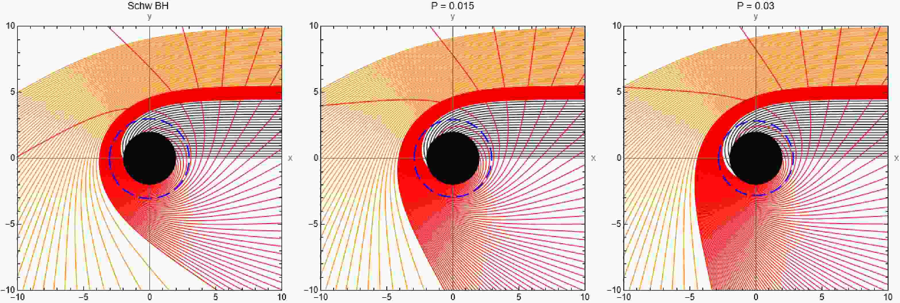
$ u_h \equiv 1/r_h $ is the inverse of the outermost horizon radius$ r_h $ , and$u_{\min}$ is the smallest positive root of$ G(u) = 0 $ . Light rays arriving at a BH from an infinitely distant source are nearly parallel. Figure 1 shows ray-tracing results near a self-dual BH in LQG, demonstrating how rays are deflected by different angles for different values of the impact parameter b. In all plots, the colors denote the following ranges: black for$ 0 \lt b \leq 4.5 $ , red for$ 4.5 \lt b \leq 5.5 $ , and orange for values of b greater than 5.5. For$ P = 0.0 $ ,$ 0.015 $ , and$ 0.03 $ , the calculated critical impact parameters are$ b_c = 5.196 $ ,$ 4.994 $ , and$ 4.803 $ , respectively. The corresponding figures show that photons with these parameters remain within the photosphere, as indicated by the blue dashed rings. As shown in the figure, the decreasing deflection angles of the red lines indicate a weakening gravitational field as the quantum correction parameter P increases.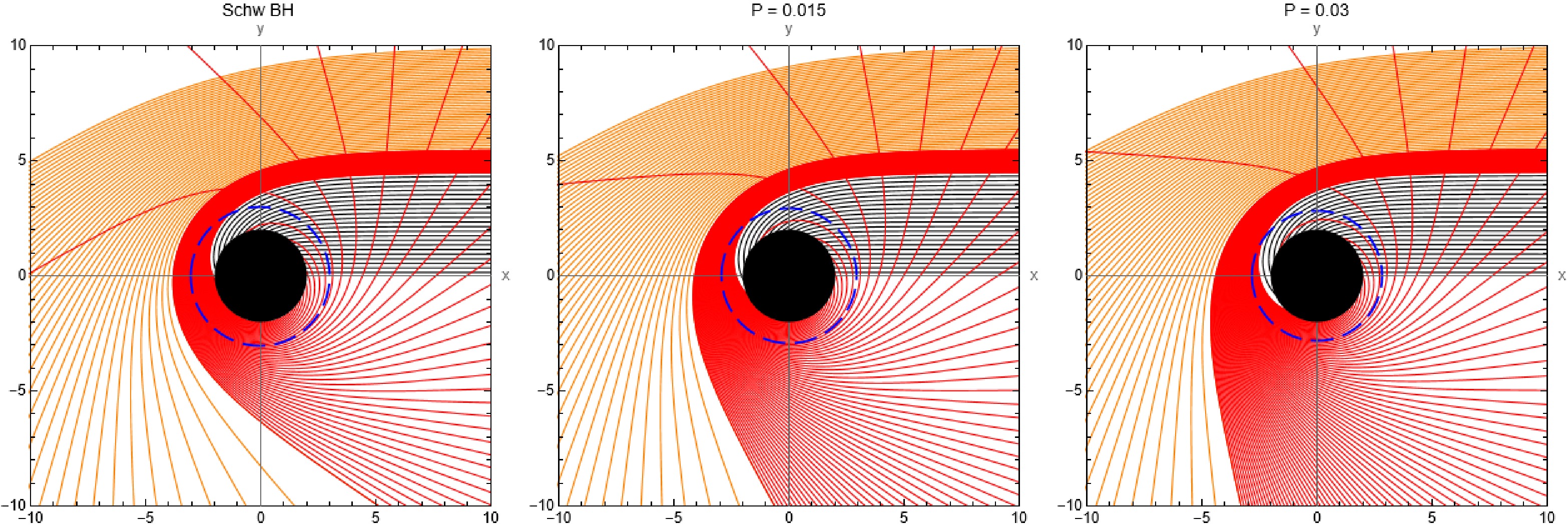
Figure 1. (color online) Photon trajectories are shown in separate plots for different values of P. In all plots, the colors are assigned as follows: black for
$ 0 \lt b \leq 4.5 $ , red for$ 4.5 \lt b \leq 5.5 $ , and orange for$ b \gt 5.5 $ . The blue dashed ring represents the photon sphere.The photon trajectories produced near the BH can be divided into three classes: direct, lensed, and photon rings [98]. The total number of orbits can be determined from the equation
$ \eta(b) = \varphi(b)/2\pi $ . To determine the boundaries of these three classes, we use the following equation [99]$ \eta = \frac{2m-1}{4}, \quad m = 1, 2, 3, \cdots\ . $
(50) Here, m is the number of intersection points, i.e., the number of times the rays cross the equatorial plane when incident along the polar axis. In Fig. 2, the number m corresponds to the number of times a ray crosses the central vertical axis. For
$ 1/4<\eta<3/4 $ , the ray crosses the axis once (direct). For$ 3/4<\eta<5/4 $ , it crosses twice (lensed). Finally, for$ \eta>5/4 $ , it crosses three or more times (photon ring).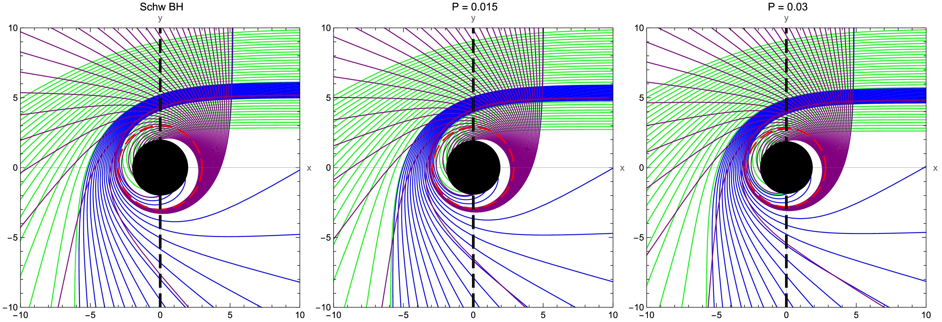
Figure 2. (color online) Photon trajectories as a function of b for self-dual black holes in LQG. The green, blue, and purple curves correspond to
$ 1/4<\eta<3/4 $ ,$ 3/4<\eta<5/4 $ , and$ \eta>5/4 $ , respectively. The red dashed ring denotes the photon sphere.For different BHs, the limiting values of the impact parameter b for the direct, lensed, and photon-ring regimes vary. These values are listed in Table 1 and correspond to the intersection points in Fig. 3. The peaks in this figure represent the critical impact parameter
$ b_c $ . As the quantum correction parameter P increases, the value of$ b_c $ decreases, indicating that the gravitational field weakens. Figure 3 corresponds to plots 1 and 3 in Fig. 2, and the same colors are used in both figures to represent the same ranges of the impact parameter b.BHs Direct ( $ 1/4 \lt \eta \lt 3/4 $ )Lensed ( $ 3/4 \lt \eta \lt 5/4 $ )Photon ring ( $ \eta \gt 5/4 $ )$ b_c $ SchwBH $ 2.848 \lt b \lt 5.015 $ and$ b \gt 6.168 $ $ 5.015 \lt b \lt 5.188 $ and$ 5.228 \lt b \lt 6.168 $ $ 5.188 \lt b \lt 5.228 $ $ 5.196 $ P = 0.015 $ 2.725 \lt b \lt 4.816 $ and$ b \gt 5.944 $ $ 4.816 \lt b \lt 4.986 $ and$ 5.026 \lt b \lt 5.944 $ $ 4.986 \lt b \lt 5.026 $ $ 4.994 $ P = 0.020 $ 2.686 \lt b \lt 4.752 $ and$ b \gt 5.873 $ $ 4.752 \lt b \lt 4.921 $ and$ 4.961 \lt b \lt 5.873 $ $ 4.921 \lt b \lt 4.961 $ 4.929 P = 0.030 $ 2.610 \lt b \lt 4.627 $ and$ b \gt 5.733 $ $ 4.627 \lt b \lt 4.794 $ and$ \ 4.835 \lt b \lt 5.733 $ $ 4.794 \lt b \lt 4.835 $ 4.803 Table 1. Classification of photon trajectories according to the impact parameter b.
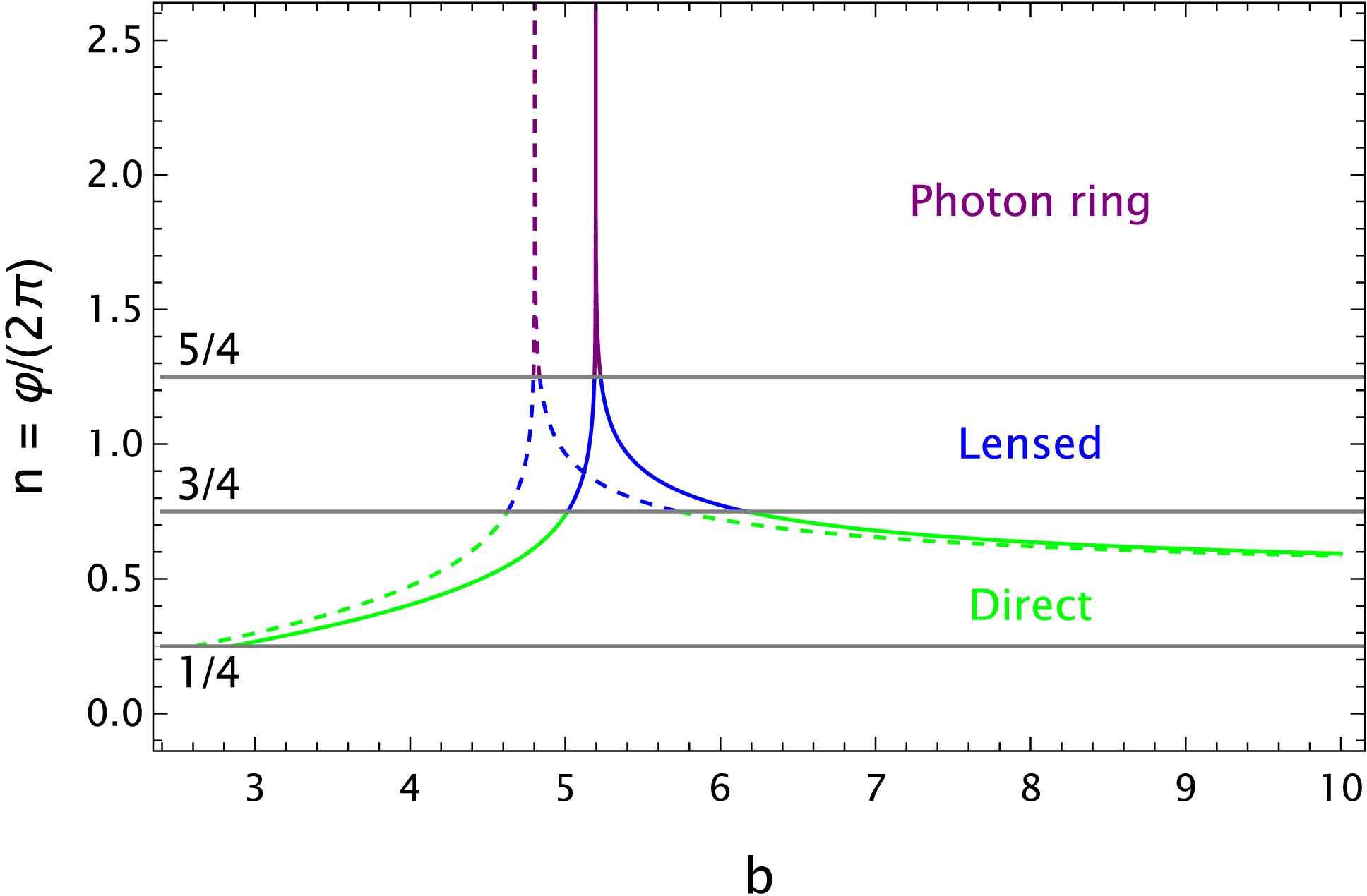
Figure 3. (color online) The plot shows the number of photon orbits, η, as a function of the impact parameter, b. The solid curve corresponds to the Schwarzschild BH, whereas the dashed curve represents the case with
$ P=0.03 $ .The trajectories can be categorized into three types [98–99]:
● Direct trajectory: The rays are deflected by an angle
$ \varphi<3\pi/2 $ , and the number of orbits satisfies$ 1/4 \lt \eta \lt 3/4 $ (green rays in Fig. 2).● Lensed trajectory: The rays are deflected through an angle in the range
$ 3\pi/2 \lt \varphi \lt 5\pi/2 $ (blue rays).● Photon ring trajectory: the number of orbits satisfies
$ \eta \gt 5/4 $ (pink rays).Table 1 shows the classification of light rays moving around self-dual BHs in LQG and their special case, the Schwarzschild BH, as a function of the impact parameter b. In the fourth column (photon ring), the light crosses the vertical axis at least three times. The central value of the interval in this column is defined by the critical impact parameter
$ b_c $ . The number of orbits η approaches infinity ($ \eta \to \infty $ ) as the impact parameter b approaches this critical value ($ b \to b_c $ ). Furthermore, if$ b \lt b_c $ , the light is absorbed by the BH. In general, as the quantum correction parameter P increases, the properties of the self-dual BH in LQG deviate more strongly from those of a Schwarzschild BH. This implies that the shadow ring and photon sphere of the self-dual BH in LQG become smaller. For example, for a Schwarzschild BH, the critical impact parameter and photon-ring interval are$ b_c\approx 5.196 $ and$ 5.188 \lt b \lt 5.228 $ , respectively. For a self-dual BH in LQG with$ P=0.03 $ , the corresponding values are$ b_c \approx 4.803 $ and$ 4.794 \lt b \lt 4.835 $ .Table 2 presents the key quantities of the LQG BH for different values of the quantum parameter P: the outer event horizon, photon sphere, and ISCO radii, as well as the critical impact parameter. Here,
$ P=0 $ corresponds to the Schwarzschild BH, while the upper limits$ P=4.3\times10^{-5} $ and$ P=0.067 $ are obtained from the perihelion shift around the Sun and Sgr$ A^* $ , respectively (see Subsec. II.B). For illustrative purposes, a larger value of the quantum parameter,$ P=0.1 $ , is also considered to better understand its effect. The table shows that, as the quantum parameter P increases, these radii and the critical impact parameter decrease. This indicates that the gravitational field becomes weaker.BHs $ r^\text{outer}_{{\rm{h}}} $ $ r_{{\rm{ph}}} $ $ b_c $ $ r_{{\rm{ISCO}}} $ $ P=0 $ $ 2 $ $ 3 $ $ 5.19615 $ $ 6 $ $ P=4.3*10^{-5} $ $ 1.99983 $ $ 2.99971 $ $ 5.19556 $ $ 5.99948 $ $ P=0.05 $ $ 1.81406 $ $ 2.6932 $ $ 4.56409 $ $ 5.45451 $ $ P=0.067 $ $ 1.75671 $ $ 2.59988 $ $ 4.37426 $ $ 5.29237 $ $ P=0.1 $ $ 1.65289 $ $ 2.43268 $ $ 4.03711 $ $ 5.01524 $ Table 2. Characteristic radii and critical impact parameter of the LQG black hole for different values of the quantum parameter P.
-
We now consider null geodesics around a self-dual BH spacetime in LQG. To this end, we first rewrite the four-momentum of a massless particle (photon) as follows:
$ p^\alpha = {\rm d}x^\alpha/{\rm d}\lambda \, . $
(36) As noted above, we restrict the photon trajectory to the equatorial plane (
$ \theta=\pi/2 $ ). Using Eqs. (10) and (36), together with the null Hamiltonian condition$ H=0 $ , we obtain the following equations of motion for light propagation:$ \frac{{\rm d}t}{{\rm d}\lambda}=\frac{E}{A(r)}, $
(37) $ \frac{{\rm d}\phi}{{\rm d}\lambda}=\frac{L}{r^2}, $
(38) $ \frac{A(r)}{B(r)}\left(\frac{{\rm d}r}{{\rm d}\lambda}\right)^2=E^2-A(r)\frac{L^2}{r^2}. $
(39) For simplicity, we apply the transformation
$ \lambda'=L\lambda $ and then rewrite the equations as$ \frac{{\rm d}t}{{\rm d}\lambda'}=\frac{1}{bA(r)}, $
(40) $ \frac{{\rm d}\phi}{{\rm d}\lambda'}=\frac{1}{r^2}\ , $
(41) $ \frac{A(r)}{B(r)}\left(\frac{{\rm d}r}{{\rm d}\lambda'}\right)^2=\frac{1}{b^2}-\frac{A(r)}{r^2}\equiv\tilde{V}_{{\rm{eff}}}(r)\ , $
(42) where
$ b=\dfrac{L}{E} $ denotes the impact parameter, and$ \tilde{V}_{{\rm{eff}}} $ denotes the normalized effective potential.The radial motion described by Eq. (42) can be written in terms of the azimuthal angle ϕ as follows:
$ \frac{A(r)}{r^4 B(r)}\left(\frac{{\rm d}r}{{\rm d}\phi}\right)^2=\frac{1}{b^2}-\frac{A(r)}{r^2}\equiv\tilde{V}_{{\rm{eff}}}(r)\, . $
(43) The photon-sphere radius is determined from the extremum of the normalized effective potential,
$ \left.\frac{{\rm d}\tilde{V}_{{\rm{eff}}}}{{\rm d}r}\right|_{r=r_{{\rm{ph}}}}=0. $
(44) Substituting the expression for
$ \tilde{V}_{{\rm{eff}}} $ yields$ \frac{{\rm d}}{{\rm d}r}\left(\frac{1}{b^2}-\frac{A(r)}{r^2}\right)=0 \quad \Rightarrow \quad rA'(r)-2A(r)=0, $
(45) The numerical solution of this equation yields the photon-sphere radius
$ r_{{\rm{ph}}} $ . Solving the condition$ \tilde{V}_{{\rm{eff}}}(r_{{\rm{ph}}})=0 $ yields the critical impact parameter$ b_c $ :$ b_c = \frac{r_{{\rm{ph}}}}{\sqrt{A(r_{{\rm{ph}}})}}. $
(46) Applying the substitution
$ r = 1/u $ to Eq. (43) yields the following equation:$ \left( \frac{{\rm d}u}{{\rm d}\phi} \right)^2 = \frac{B(u)}{A(u)b^2} - u^2 B\left(u \right)\equiv G(u). $
(47) Using Eq. (16), we obtain the following equation:
$ \begin{split} G(u)=&\dfrac{1}{b^2 u^4 \left(\dfrac{2 P}{(P+1)^2}+\dfrac{1}{u}\right)^4}\\&-\dfrac{u^2 \left(\dfrac{1}{u}-\dfrac{2}{(P+1)^2}\right) \left(\dfrac{1}{u}-\dfrac{2 P^2}{(P+1)^2}\right)}{\left(\dfrac{2 P}{(P+1)^2}+\dfrac{1}{u}\right)^2}\ . \end{split} $
(48) The total change in the azimuthal angle φ is given by a piecewise function that depends on the impact parameter:
$ \varphi = \left\{\begin{array}{*{20}{l}} \ \ \ \displaystyle\int\nolimits_0^{u_h} \dfrac{{\rm d}u}{\sqrt{G(u)}}\ , \quad & b \lt b_c\ \\ 2 \displaystyle\int\nolimits_0^{u_{\min}} \dfrac{{\rm d}u}{\sqrt{G(u)}}\ , \quad & b \gt b_c\ , \end{array}\right. $
(49) where
$ u_h \equiv 1/r_h $ is the inverse of the outermost horizon radius$ r_h $ , and$u_{\min}$ is the smallest positive root of$ G(u) = 0 $ . Light rays arriving at a BH from an infinitely distant source are nearly parallel. Figure 1 shows ray-tracing results near a self-dual BH in LQG, demonstrating how rays are deflected by different angles for different values of the impact parameter b. In all plots, the colors denote the following ranges: black for$ 0 \lt b \leq 4.5 $ , red for$ 4.5 \lt b \leq 5.5 $ , and orange for values of b greater than 5.5. For$ P = 0.0 $ ,$ 0.015 $ , and$ 0.03 $ , the calculated critical impact parameters are$ b_c = 5.196 $ ,$ 4.994 $ , and$ 4.803 $ , respectively. The corresponding figures show that photons with these parameters remain within the photosphere, as indicated by the blue dashed rings. As shown in the figure, the decreasing deflection angles of the red lines indicate a weakening gravitational field as the quantum correction parameter P increases.
Figure 1. (color online) Photon trajectories are shown in separate plots for different values of P. In all plots, the colors are assigned as follows: black for
$ 0 \lt b \leq 4.5 $ , red for$ 4.5 \lt b \leq 5.5 $ , and orange for$ b \gt 5.5 $ . The blue dashed ring represents the photon sphere.The photon trajectories produced near the BH can be divided into three classes: direct, lensed, and photon rings [98]. The total number of orbits can be determined from the equation
$ \eta(b) = \varphi(b)/2\pi $ . To determine the boundaries of these three classes, we use the following equation [99]$ \eta = \frac{2m-1}{4}, \quad m = 1, 2, 3, \cdots\ . $
(50) Here, m is the number of intersection points, i.e., the number of times the rays cross the equatorial plane when incident along the polar axis. In Fig. 2, the number m corresponds to the number of times a ray crosses the central vertical axis. For
$ 1/4<\eta<3/4 $ , the ray crosses the axis once (direct). For$ 3/4<\eta<5/4 $ , it crosses twice (lensed). Finally, for$ \eta>5/4 $ , it crosses three or more times (photon ring).
Figure 2. (color online) Photon trajectories as a function of b for self-dual black holes in LQG. The green, blue, and purple curves correspond to
$ 1/4<\eta<3/4 $ ,$ 3/4<\eta<5/4 $ , and$ \eta>5/4 $ , respectively. The red dashed ring denotes the photon sphere.For different BHs, the limiting values of the impact parameter b for the direct, lensed, and photon-ring regimes vary. These values are listed in Table 1 and correspond to the intersection points in Fig. 3. The peaks in this figure represent the critical impact parameter
$ b_c $ . As the quantum correction parameter P increases, the value of$ b_c $ decreases, indicating that the gravitational field weakens. Figure 3 corresponds to plots 1 and 3 in Fig. 2, and the same colors are used in both figures to represent the same ranges of the impact parameter b.BHs Direct ( $ 1/4 \lt \eta \lt 3/4 $ )Lensed ( $ 3/4 \lt \eta \lt 5/4 $ )Photon ring ( $ \eta \gt 5/4 $ )$ b_c $ SchwBH $ 2.848 \lt b \lt 5.015 $ and$ b \gt 6.168 $ $ 5.015 \lt b \lt 5.188 $ and$ 5.228 \lt b \lt 6.168 $ $ 5.188 \lt b \lt 5.228 $ $ 5.196 $ P = 0.015 $ 2.725 \lt b \lt 4.816 $ and$ b \gt 5.944 $ $ 4.816 \lt b \lt 4.986 $ and$ 5.026 \lt b \lt 5.944 $ $ 4.986 \lt b \lt 5.026 $ $ 4.994 $ P = 0.020 $ 2.686 \lt b \lt 4.752 $ and$ b \gt 5.873 $ $ 4.752 \lt b \lt 4.921 $ and$ 4.961 \lt b \lt 5.873 $ $ 4.921 \lt b \lt 4.961 $ 4.929 P = 0.030 $ 2.610 \lt b \lt 4.627 $ and$ b \gt 5.733 $ $ 4.627 \lt b \lt 4.794 $ and$ \ 4.835 \lt b \lt 5.733 $ $ 4.794 \lt b \lt 4.835 $ 4.803 Table 1. Classification of photon trajectories according to the impact parameter b.
Figure 3. (color online) The plot shows the number of photon orbits, η, as a function of the impact parameter, b. The solid curve corresponds to the Schwarzschild BH, whereas the dashed curve represents the case with
$ P=0.03 $ .The trajectories can be categorized into three types [98–99]:
● Direct trajectory: The rays are deflected by an angle
$ \varphi<3\pi/2 $ , and the number of orbits satisfies$ 1/4 \lt \eta \lt 3/4 $ (green rays in Fig. 2).● Lensed trajectory: The rays are deflected through an angle in the range
$ 3\pi/2 \lt \varphi \lt 5\pi/2 $ (blue rays).● Photon ring trajectory: the number of orbits satisfies
$ \eta \gt 5/4 $ (pink rays).Table 1 shows the classification of light rays moving around self-dual BHs in LQG and their special case, the Schwarzschild BH, as a function of the impact parameter b. In the fourth column (photon ring), the light crosses the vertical axis at least three times. The central value of the interval in this column is defined by the critical impact parameter
$ b_c $ . The number of orbits η approaches infinity ($ \eta \to \infty $ ) as the impact parameter b approaches this critical value ($ b \to b_c $ ). Furthermore, if$ b \lt b_c $ , the light is absorbed by the BH. In general, as the quantum correction parameter P increases, the properties of the self-dual BH in LQG deviate more strongly from those of a Schwarzschild BH. This implies that the shadow ring and photon sphere of the self-dual BH in LQG become smaller. For example, for a Schwarzschild BH, the critical impact parameter and photon-ring interval are$ b_c\approx 5.196 $ and$ 5.188 \lt b \lt 5.228 $ , respectively. For a self-dual BH in LQG with$ P=0.03 $ , the corresponding values are$ b_c \approx 4.803 $ and$ 4.794 \lt b \lt 4.835 $ .Table 2 presents the key quantities of the LQG BH for different values of the quantum parameter P: the outer event horizon, photon sphere, and ISCO radii, as well as the critical impact parameter. Here,
$ P=0 $ corresponds to the Schwarzschild BH, while the upper limits$ P=4.3\times10^{-5} $ and$ P=0.067 $ are obtained from the perihelion shift around the Sun and Sgr$ A^* $ , respectively (see Subsec. II.B). For illustrative purposes, a larger value of the quantum parameter,$ P=0.1 $ , is also considered to better understand its effect. The table shows that, as the quantum parameter P increases, these radii and the critical impact parameter decrease. This indicates that the gravitational field becomes weaker.BHs $ r^\text{outer}_{{\rm{h}}} $ $ r_{{\rm{ph}}} $ $ b_c $ $ r_{{\rm{ISCO}}} $ $ P=0 $ $ 2 $ $ 3 $ $ 5.19615 $ $ 6 $ $ P=4.3*10^{-5} $ $ 1.99983 $ $ 2.99971 $ $ 5.19556 $ $ 5.99948 $ $ P=0.05 $ $ 1.81406 $ $ 2.6932 $ $ 4.56409 $ $ 5.45451 $ $ P=0.067 $ $ 1.75671 $ $ 2.59988 $ $ 4.37426 $ $ 5.29237 $ $ P=0.1 $ $ 1.65289 $ $ 2.43268 $ $ 4.03711 $ $ 5.01524 $ Table 2. Characteristic radii and critical impact parameter of the LQG black hole for different values of the quantum parameter P.
-
In this section, we investigate the radiative properties of an accretion disk composed of gas, dust, and plasma orbiting a self-dual BH in LQG. A widely used theoretical framework for describing such disks is the Novikov–Thorne model [100, 78], which treats the disk as optically thick and geometrically thin. In this approximation, the vertical thickness h is much smaller than the radial extent r, i.e.,
$ h \ll r $ , and can therefore be neglected relative to the disk's radial size. Observationally, accretion disks are typically characterized by their electromagnetic flux, temperature distribution, and luminosity. In what follows, we analyze in detail the influence of the quantum-correction parameter P on the image, energy flux, and redshift.For the purpose of analyzing the image of a thin accretion disk, we use an observational coordinate system, as depicted in Fig. 4. In this setup, the observer is located at
$ (\infty, \theta, 0) $ in the spherical coordinate system of the BH,$ (r, \theta, \phi) $ , whose origin$ (r=0) $ is defined at the center of the BH.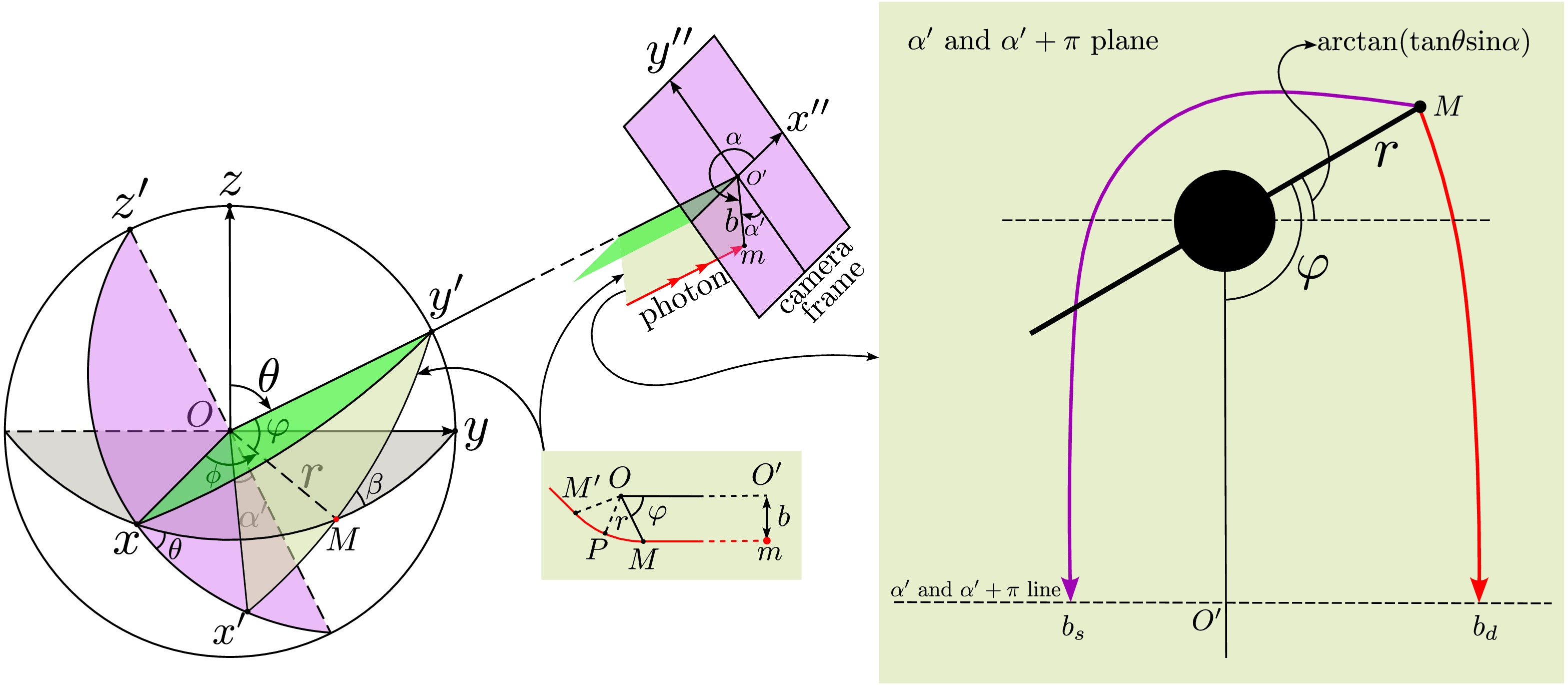
Figure 4. (color online) Schematic representation of the coordinate system used to construct the image of the accretion disk.
Assume that, in the observer's coordinate system
$ O'x''y'' $ (the camera frame), a photon is emitted from the point$ m(b,\alpha) $ and propagates perpendicular to the camera plane toward the BH, intersecting the disk at the point$ M(r,\pi/2,\phi) $ . According to the principle of optical path reversibility, a photon emitted from$ M(r,\pi/2,\phi) $ on the accretion disk follows a trajectory that arrives at the image point$ m(b,\alpha) $ in the camera frame. In our analysis, we consider two types of images. The direct image$ (b_d,\alpha) $ is generated by photons that propagate directly from the disk toward the observer's camera. In contrast, the secondary image$ (b_s,\alpha+\pi) $ arises from photons that initially move in the opposite direction but are bent around the BH by gravitational lensing before reaching the observer (see the right panel of Fig. 4).By applying the sine theorem for spherical triangles to
$ \triangle Myy' $ and$ \triangle Mxx' $ , we obtain the following relations:$ \dfrac{\sin(\varphi)}{\sin\left(\dfrac{\pi}{2}\right)} = \dfrac{\sin\left(\dfrac{\pi}{2}-\theta\right)}{\sin(\beta)}\, , $
(51) $ \dfrac{\sin\left(\dfrac{\pi}{2}-\varphi\right)}{\sin(\theta)} = \dfrac{\sin\left(\dfrac{\pi}{2}-\alpha\right)}{\sin(\beta)}\, . $
(52) Using the relations above, together with
$ \alpha+\alpha' = 3\pi/2 $ , the deflection angle φ can be expressed as follows:$ \varphi = \frac{\pi}{2} + \arctan(\tan\theta \sin\alpha). $
(53) The angular deflections associated with the formation of the
$ n^{\text{th}} $ -order image, denoted by$ \varphi_n $ , are given by [101]$ \begin{aligned}[b] & \varphi_n =\\ &\left\{\begin{array}{*{20}{l}} \dfrac{n}{2} 2\pi + (-1)^n \left[ \dfrac{\pi}{2} + \arctan(\tan\theta \sin\alpha) \right], & \text{for } n \text{ even}, \\ \dfrac{n+1}{2} 2\pi + (-1)^n \left[ \dfrac{\pi}{2} + \arctan(\tan\theta \sin\alpha) \right], & \text{for } n \text{ odd} \, , \end{array}\right. \end{aligned} $
(54) where
$ n=0 $ and$ n=1 $ correspond to the direct and secondary images, respectively. Suppose that a photon is emitted from the camera plane at infinity, with coordinates$ (b,\alpha) $ , and reaches a circular orbit of radius r in the black hole accretion disk. In this case, the total deflection angle of the photon along its trajectory can be expressed as$ \varphi_1(b) = \int^{u_r}_{0} \frac{1}{\sqrt{G(u)}} {\rm d}u, $
(55) $ \varphi_2(b) = 2 \int^{u_{\min}}_{0} \frac{1}{\sqrt{G(u)}} {\rm d}u - \int^{u_r}_{0} \frac{1}{\sqrt{G(u)}} {\rm d}u. $
(56) Figure 5 illustrates the dependence of the photon deflection angle φ on the impact parameter b. The left panel shows the integral curves
$ \varphi_1 $ and$ \varphi_2 $ for different values of the quantum correction parameter P. The peaks correspond to the critical values$ b_c $ of the impact parameter. It is evident that$ b_c $ decreases significantly as P increases. Interestingly, as P increases, the impact parameter b decreases more significantly in the$ n\geq1 $ region than in the$ n=0 $ region, indicating that the decrease rate for secondary images is slightly larger than that for direct images. It should be noted that the curve for$ P=0 $ corresponds to the Schwarzschild BH case. In the right panel of Fig. 5, the blue dashed curve corresponds to the photon deflection angle$ \varphi_3 $ at the periastron (i.e., the point of closest approach to the BH for a given trajectory), which is determined by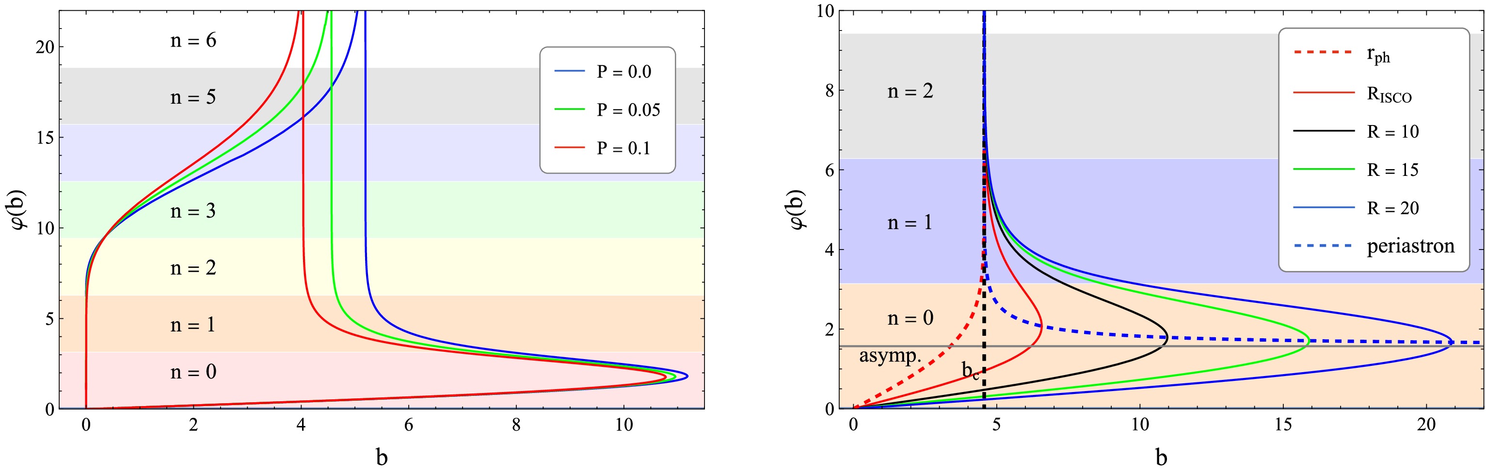
Figure 5. (color online) Image formation diagrams for various values of the quantum correction parameter P at fixed radius
$ R=10 $ (left panel) and for various values of the radius R at fixed$ P=0.05 $ (right panel). The innermost stable circular orbit is at$ R_{\rm ISCO}=5.455 $ , corresponding to the solid red curve.$ \varphi_3(b) = \int^{u_{\min}}_{0} \frac{1}{\sqrt{G(u)}} {\rm d}u\, . $
(57) Note that the blue dashed curve asymptotically approaches the line
$ \varphi=\pi/2 $ , below which the curves correspond to$ \varphi_1 $ , whereas above it they correspond to$ \varphi_2 $ . The intersection point of the curves corresponding to$ \varphi_1 $ ,$ \varphi_2 $ , and$ \varphi_3 $ gives the maximum impact parameter$b_{\max}$ . As the radius R increases,$b_{\max}$ increases accordingly. The colored regions demarcate the boundaries of the direct$ (n=0) $ and$ n^{\text{th}} $ -order images. The accretion disk extends from$R_{\rm ISCO}$ to its outer edge. For light from larger disk radii$ (R = 10, 15, 20) $ to reach the observer, the rays must have correspondingly larger impact parameters, as shown in the right panel of Fig. 4. We find that the maximum impact parameters for these radii are$b_{\max} =$ 10.96, 15.90, and 20.88, respectively. We also observe that the secondary$ (n \geq 1) $ images of rays originating from various radii remain almost unchanged compared with the direct image$ (n = 0) $ .In this work, we use a semi-analytic ray-tracing algorithm based on the optical path reversibility principle to obtain accretion disk images. The numerical integrations were performed with an accuracy of
$ 10^{-10} $ . The image order is determined by the number of times the photon crosses the plane of the accretion disk before reaching the observer. If a photon reaches the event horizon, it is considered to be captured by the BH, and the ray-tracing calculation is terminated. If the photon reaches a turning point, its radial direction reverses, and it continues propagating away from the BH.After numerically solving Eqs. (54), (55), and (56) for the primary and secondary images, we obtain the coordinates
$ (b,\alpha) $ of the accretion disk in the observer's plane [69, 81]. In Fig. 6, the direct and secondary images of stable circular orbits around a self-dual BH in LQG, as observed by a distant observer, are shown for different inclination angles. From Fig. 6, it is evident that increasing the quantum correction parameter P (from left to right along each row) reduces the size of both the primary and secondary images. This implies that, as P increases, a smaller impact parameter b is required for photons to reach the same stationary circular orbit, indicating a weakening of the gravitational field.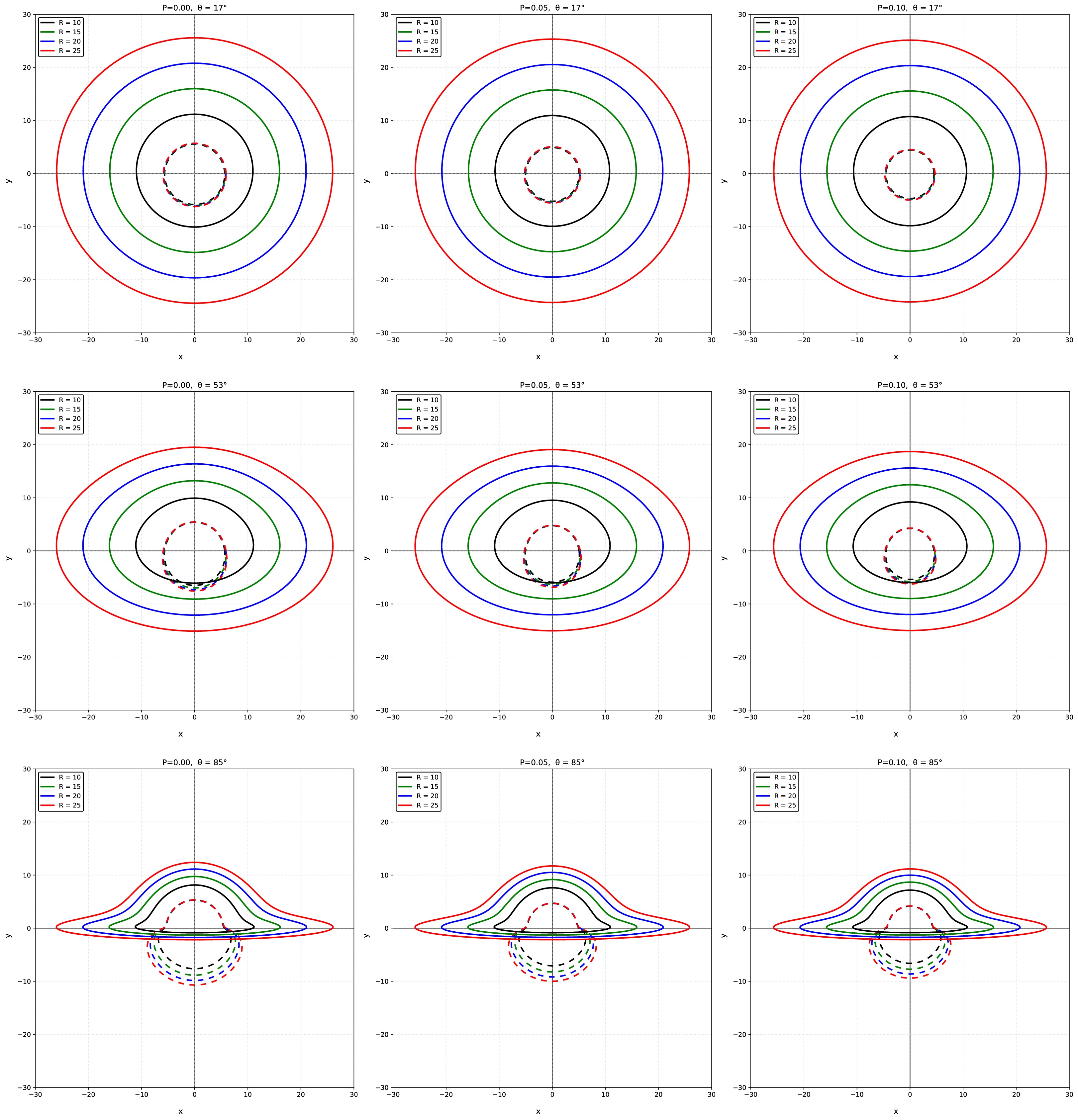
Figure 6. (color online) Direct and secondary images of the thin accretion disk around a self-dual BH in LQG. From top to bottom, the rows represent inclination angles of
$ 17^\circ $ ,$ 53^\circ $ , and$ 85^\circ $ ; from left to right, the columns correspond to P values of 0.0, 0.05, and 0.10.The emitting matter moves on circular geodesic orbits in the equatorial plane, with four-velocity
$ u^\alpha_{{\rm{em}}} = u^t(1,0,0,\Omega) $ normalized by$ g_{\alpha\beta}u^\alpha u^\beta = -1 $ , where Ω is given by Eq. (61). The quantities E and L in Eqs. (59)–(60) follow from this normalization. The distant observer is static at infinity, with$ u^\alpha_{{\rm{obs}}} = (1,0,0,0) $ .The surface radiative energy flux is given by [102−104]
$ F(r) = -\frac{\dot{M}_0 \Omega_{,r}}{4\pi \sqrt{-g}(E - \Omega L)^2} \int_{r_{\text{isco}}}^{r} (E - \Omega L)L_{,r} {\rm d}r\, , $
(58) where
$ \dot{M}_0 $ denotes the mass accretion rate, g is the determinant of the spacetime metric, and E, L, and Ω denote the energy, angular momentum, and angular velocity, respectively, of a particle in a circular orbit. For a particle in a circular orbit around a static, spherically symmetric BH, these quantities are defined as follows [105, 106]:$ E = -\frac{g_{tt}}{\sqrt{-g_{tt} - g_{\phi\phi}\Omega^2}}, $
(59) $ L = \frac{g_{\phi\phi}\Omega}{\sqrt{-g_{tt} - g_{\phi\phi}\Omega^2}}, $
(60) $ \Omega = \frac{{\rm d}\phi}{{\rm d}t} = \sqrt{-\frac{g_{tt,r}}{g_{\phi\phi,r}}}. $
(61) The expressions for E, L, and Ω are written in terms of the metric functions
$ g_{tt} $ and$ g_{\phi\phi} $ of the self-dual BH metric. The full metric has$ g_{\phi\phi} = C(r)\sin^2\theta $ , where$ C(r) = r^2 + a_0^2/r^2 $ . Since$ a_0 \propto l_{Pl}^2 $ is negligibly small, we set$ a_0 = 0 $ (Sec. 2), which restores$ C(r) = r^2 $ and justifies the use of the standard disk formulae. Accordingly,$ \sqrt{-g} = r^2\sin\theta\sqrt{A(r)/B(r)} $ at$ \theta = \pi/2 $ . The accretion rate is set to$ \dot{M}_0 = 1 $ throughout; thus, the flux profiles$ F(r) $ are expressed in geometrized units, and this normalization does not affect the qualitative comparison with the Schwarzschild case.Table 3 summarizes the main quantities of the accretion disk around the BH in LQG for several values of the quantum parameter P. The table lists the ISCO radius, the specific energy, and the corresponding radiative efficiency,
$ \eta_{{\rm{ef}}} $ . Increasing P causes the ISCO radius to shift inward, whereas the specific energy,$ E_{{\rm{ISCO}}} $ , increases. The radiative efficiency, calculated as$ \eta_{{\rm{ef}}}=1-E_{{\rm{ISCO}}} $ , is shown in the last column. Thus, higher values of the quantum parameter lead to lower radiative efficiency.BHs $ r_{{\rm{ISCO}}} $ $ E_{{\rm{ISCO}}} $ $ \eta_{{\rm{ef}}} $ $ P=0 $ $ 6 $ $ 0.943 $ 5.72% $ P=0.05 $ $ 5.45451 $ $ 0.948 $ 5.19% $ P=0.1 $ $ 5.01524 $ $ 0.953 $ 4.66% Table 3. Characteristic quantities of the accretion disk around a BH in LQG for different values of the quantum parameter P.
Figure 7 shows the energy flux
$ F(r) $ of a self-dual BH in LQG as a function of the radius r for different values of the quantum correction parameter P. The figure indicates that increasing P enhances the peak of the energy flux$ F(r) $ and shifts it toward smaller radii.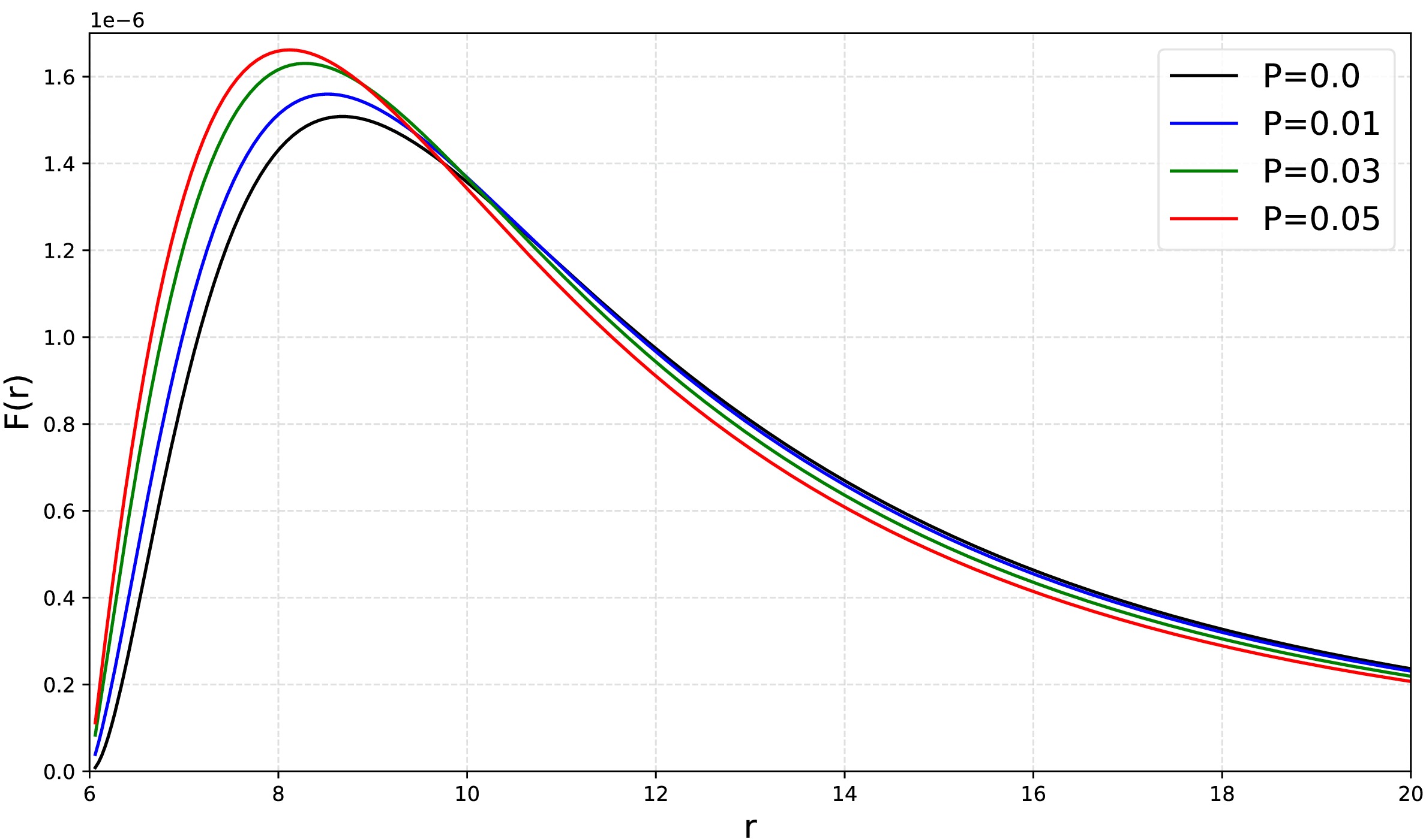
Figure 7. (color online) Energy flux
$ F(r) $ as a function of the radius r for different values of the quantum correction parameter P.At infinity, the observed radiation flux is affected by both gravitational redshift and Doppler effects. As shown in Ref. [107], it is given by:
$ F_{\text{obs}} = \frac{F(r)}{(1+z)^4}, $
(62) The photon four-momentum
$ p^\alpha_{{\rm{ph}}} $ satisfies$ p_t^{{\rm{ph}}} = -E_{{\rm{ph}}} $ and$ p_\phi^{{\rm{ph}}} = L_{{\rm{ph}}} $ , with impact parameter$ b = L_{{\rm{ph}}}/E_{{\rm{ph}}} $ (Eqs. (37) and (38)). The redshift factor is generally defined as$ 1+z = \dfrac{-(p_\alpha^{{\rm{ph}}} u^\alpha)_{{\rm{em}}}}{-(p_\alpha^{{\rm{ph}}} u^\alpha)_{{\rm{obs}}}} $ . Substituting the emitter's four-velocity and the geometric relation between the impact parameter b and the local photon propagation direction at the emission point—obtained from the observer angles$ \theta,\alpha $ , as specified at the beginning of Sec. IV (see Fig. 4)—we obtain the following expression [108]:$ 1 + z = \frac{1 + \Omega b \sin \theta \cos\alpha}{\sqrt{-g_{tt} - g_{\phi\phi}\Omega^2}}. $
(63) The flux
$ F(r) $ in Eq. (58) follows the standard Novikov–Thorne formalism for a thin, optically thick disk radiating as a local blackbody and is derived from conservation laws with constant$ \dot{M}_0 $ . It is not a full radiative-transfer calculation. Thus,$ F(r) $ and$ F_{{\rm{obs}}} $ are theoretical diagnostic quantities.We apply the same method as in Fig. 6 to orbits from
$ R_{\text{isco}} $ to$ R=25 $ . Assigning colors to the observed flux$ F_{\text{obs}} $ and the redshift factor z corresponding to each$ (b,\alpha) $ yields their distributions across the accretion disk of a self-dual BH in LQG (see Fig. 8 and Fig. 9). Figure 8 shows the distribution of$ F_{\text{obs}} $ for various inclination angles and values of P. The figure indicates that a self-dual BH in LQG and a Schwarzschild BH ($ P=0 $ ) exhibit similar$ F_{\text{obs}} $ distributions. The key distinction is that the self-dual BH appears smaller and brighter than the Schwarzschild case. If the observed energy flux$ F_{\text{obs}} $ of the self-dual BH in LQG at$ P = 0.1 $ and$ \theta = 85^\circ $ is normalized to 100%, then the observed energy flux of the Schwarzschild BH at the same inclination is about 80%, as shown in the bottom row of Fig. 8.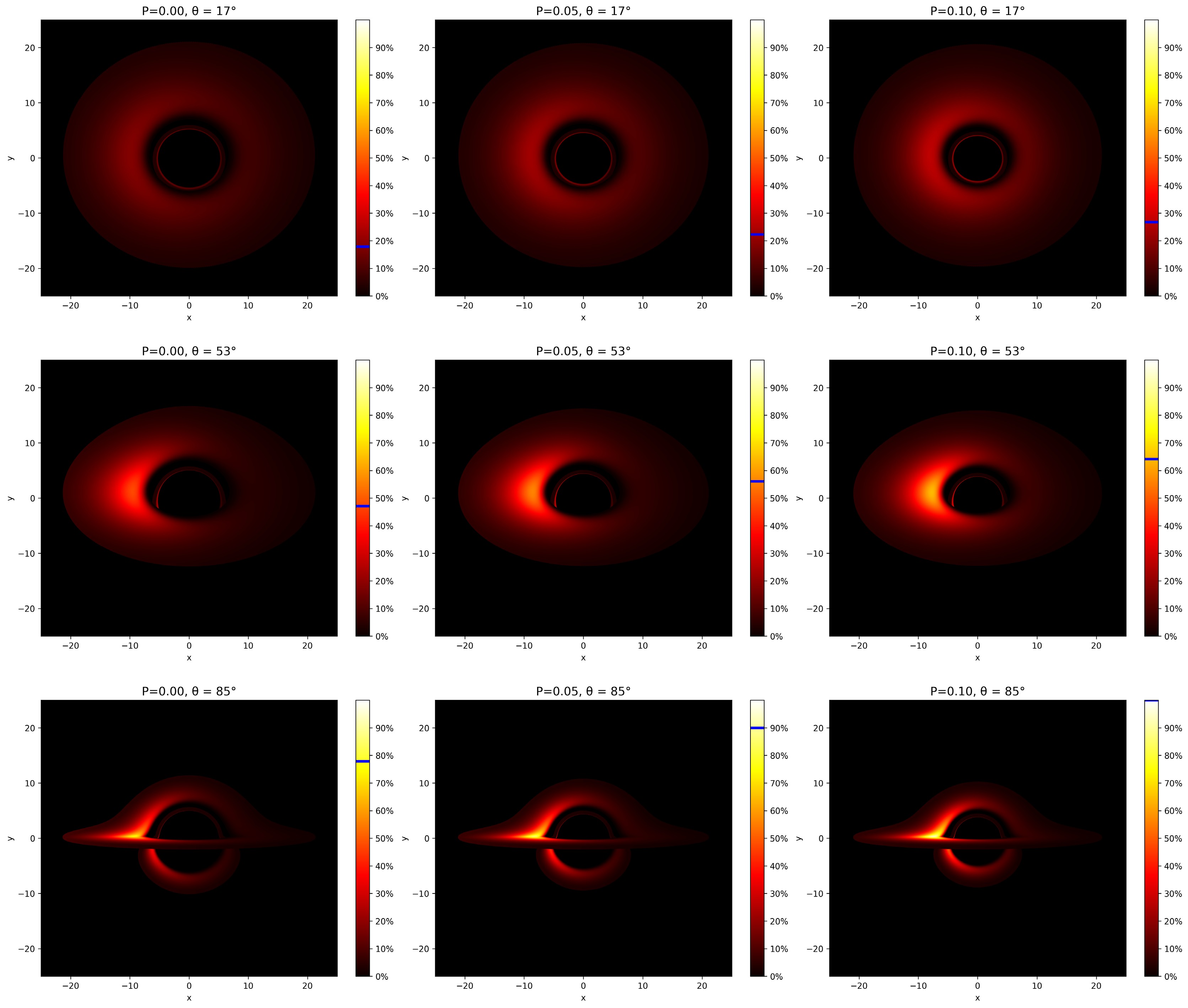
Figure 8. (color online) Distribution of the observed flux
$ F_{\text{obs}} $ in the direct and secondary images of a self-dual BH in LQG for inclination angles of$ 17^\circ $ ,$ 53^\circ $ , and$ 85^\circ $ .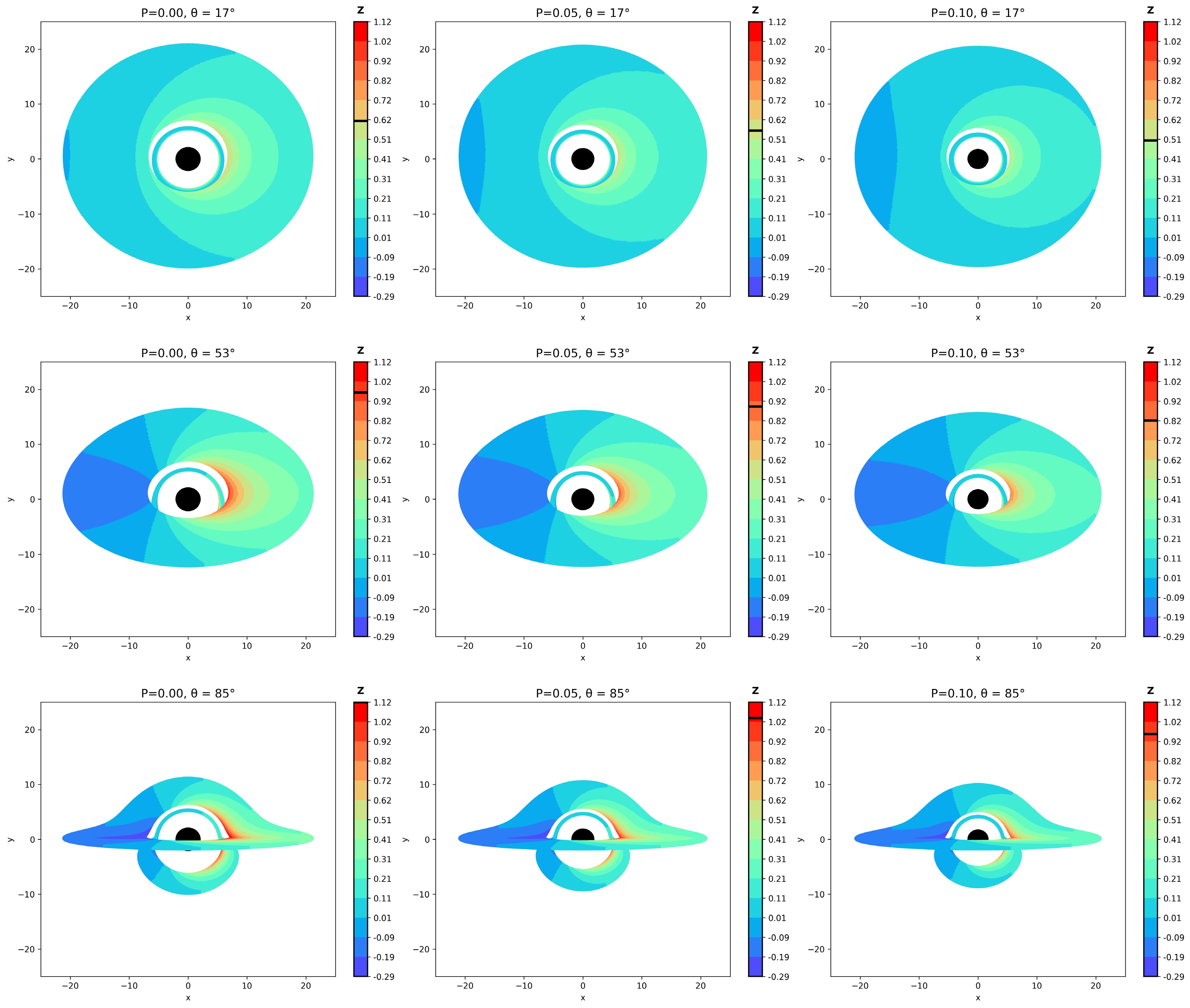
Figure 9. (color online) The distributions of the redshift factor z for the direct and secondary images of a self-dual BH in LQG are shown for inclination angles of
$ 17^\circ $ ,$ 53^\circ $ , and$ 85^\circ $ .Figure 9 shows the redshift distribution of the accretion disk for different inclination angles. If only gravitational redshift were present, the redshift (
$ z>0 $ ) distribution would be symmetric. However, disk rotation introduces a Doppler contribution, making the distribution asymmetric. On the side rotating toward the observer, the redshift is reduced and may even become a blueshift ($ z<0 $ ), whereas on the opposite side the redshift is amplified. The black line on the color bar indicates the maximum redshift for each disk. For$ P=0.0 $ ,$ \theta=85^\circ $ , the values$z_{\max}=1.12$ and$z_{\min}=-0.29$ are obtained. These correspond to the most extreme values among all cases. The viewing angle also affects the distribution, with stronger redshift effects appearing at higher inclinations. These results indicate that the redshift patterns of the self-dual BH in LQG and the Schwarzschild BH ($ P=0 $ ) are similar, although the effects are slightly weaker for the self-dual BH case. Such differences could serve as potential observational signatures for distinguishing BH geometries.We also note that the present analysis is restricted to the static, nonrotating self-dual BH in LQG. Since realistic astrophysical BHs have non-negligible spin, extending this study to a rotating self-dual BH would be necessary for a more direct comparison with observations, and we leave this for future work.
The accretion-disk images, flux, and redshift profiles presented in this section constitute theoretical predictions for the image morphology and disk observables of the self-dual BH in LQG, rather than direct observational constraints. This work does not include image fitting or plasma radiative-transfer modeling, and no direct comparison with observational data (e.g., from EHT) has been carried out.
-
In this section, we investigate the radiative properties of an accretion disk composed of gas, dust, and plasma orbiting a self-dual BH in LQG. A widely used theoretical framework for describing such disks is the Novikov–Thorne model [100, 78], which treats the disk as optically thick and geometrically thin. In this approximation, the vertical thickness h is much smaller than the radial extent r, i.e.,
$ h \ll r $ , and can therefore be neglected relative to the disk's radial size. Observationally, accretion disks are typically characterized by their electromagnetic flux, temperature distribution, and luminosity. In what follows, we analyze in detail the influence of the quantum-correction parameter P on the image, energy flux, and redshift.For the purpose of analyzing the image of a thin accretion disk, we use an observational coordinate system, as depicted in Fig. 4. In this setup, the observer is located at
$ (\infty, \theta, 0) $ in the spherical coordinate system of the BH,$ (r, \theta, \phi) $ , whose origin$ (r=0) $ is defined at the center of the BH.
Figure 4. (color online) Schematic representation of the coordinate system used to construct the image of the accretion disk.
Assume that, in the observer's coordinate system
$ O'x''y'' $ (the camera frame), a photon is emitted from the point$ m(b,\alpha) $ and propagates perpendicular to the camera plane toward the BH, intersecting the disk at the point$ M(r,\pi/2,\phi) $ . According to the principle of optical path reversibility, a photon emitted from$ M(r,\pi/2,\phi) $ on the accretion disk follows a trajectory that arrives at the image point$ m(b,\alpha) $ in the camera frame. In our analysis, we consider two types of images. The direct image$ (b_d,\alpha) $ is generated by photons that propagate directly from the disk toward the observer's camera. In contrast, the secondary image$ (b_s,\alpha+\pi) $ arises from photons that initially move in the opposite direction but are bent around the BH by gravitational lensing before reaching the observer (see the right panel of Fig. 4).By applying the sine theorem for spherical triangles to
$ \triangle Myy' $ and$ \triangle Mxx' $ , we obtain the following relations:$ \dfrac{\sin(\varphi)}{\sin\left(\dfrac{\pi}{2}\right)} = \dfrac{\sin\left(\dfrac{\pi}{2}-\theta\right)}{\sin(\beta)}\, , $
(51) $ \dfrac{\sin\left(\dfrac{\pi}{2}-\varphi\right)}{\sin(\theta)} = \dfrac{\sin\left(\dfrac{\pi}{2}-\alpha\right)}{\sin(\beta)}\, . $
(52) Using the relations above, together with
$ \alpha+\alpha' = 3\pi/2 $ , the deflection angle φ can be expressed as follows:$ \varphi = \frac{\pi}{2} + \arctan(\tan\theta \sin\alpha). $
(53) The angular deflections associated with the formation of the
$ n^{\text{th}} $ -order image, denoted by$ \varphi_n $ , are given by [101]$ \begin{aligned}[b] & \varphi_n =\\ &\left\{\begin{array}{*{20}{l}} \dfrac{n}{2} 2\pi + (-1)^n \left[ \dfrac{\pi}{2} + \arctan(\tan\theta \sin\alpha) \right], & \text{for } n \text{ even}, \\ \dfrac{n+1}{2} 2\pi + (-1)^n \left[ \dfrac{\pi}{2} + \arctan(\tan\theta \sin\alpha) \right], & \text{for } n \text{ odd} \, , \end{array}\right. \end{aligned} $
(54) where
$ n=0 $ and$ n=1 $ correspond to the direct and secondary images, respectively. Suppose that a photon is emitted from the camera plane at infinity, with coordinates$ (b,\alpha) $ , and reaches a circular orbit of radius r in the black hole accretion disk. In this case, the total deflection angle of the photon along its trajectory can be expressed as$ \varphi_1(b) = \int^{u_r}_{0} \frac{1}{\sqrt{G(u)}} {\rm d}u, $
(55) $ \varphi_2(b) = 2 \int^{u_{\min}}_{0} \frac{1}{\sqrt{G(u)}} {\rm d}u - \int^{u_r}_{0} \frac{1}{\sqrt{G(u)}} {\rm d}u. $
(56) Figure 5 illustrates the dependence of the photon deflection angle φ on the impact parameter b. The left panel shows the integral curves
$ \varphi_1 $ and$ \varphi_2 $ for different values of the quantum correction parameter P. The peaks correspond to the critical values$ b_c $ of the impact parameter. It is evident that$ b_c $ decreases significantly as P increases. Interestingly, as P increases, the impact parameter b decreases more significantly in the$ n\geq1 $ region than in the$ n=0 $ region, indicating that the decrease rate for secondary images is slightly larger than that for direct images. It should be noted that the curve for$ P=0 $ corresponds to the Schwarzschild BH case. In the right panel of Fig. 5, the blue dashed curve corresponds to the photon deflection angle$ \varphi_3 $ at the periastron (i.e., the point of closest approach to the BH for a given trajectory), which is determined by
Figure 5. (color online) Image formation diagrams for various values of the quantum correction parameter P at fixed radius
$ R=10 $ (left panel) and for various values of the radius R at fixed$ P=0.05 $ (right panel). The innermost stable circular orbit is at$ R_{\rm ISCO}=5.455 $ , corresponding to the solid red curve.$ \varphi_3(b) = \int^{u_{\min}}_{0} \frac{1}{\sqrt{G(u)}} {\rm d}u\, . $
(57) Note that the blue dashed curve asymptotically approaches the line
$ \varphi=\pi/2 $ , below which the curves correspond to$ \varphi_1 $ , whereas above it they correspond to$ \varphi_2 $ . The intersection point of the curves corresponding to$ \varphi_1 $ ,$ \varphi_2 $ , and$ \varphi_3 $ gives the maximum impact parameter$b_{\max}$ . As the radius R increases,$b_{\max}$ increases accordingly. The colored regions demarcate the boundaries of the direct$ (n=0) $ and$ n^{\text{th}} $ -order images. The accretion disk extends from$R_{\rm ISCO}$ to its outer edge. For light from larger disk radii$ (R = 10, 15, 20) $ to reach the observer, the rays must have correspondingly larger impact parameters, as shown in the right panel of Fig. 4. We find that the maximum impact parameters for these radii are$b_{\max} =$ 10.96, 15.90, and 20.88, respectively. We also observe that the secondary$ (n \geq 1) $ images of rays originating from various radii remain almost unchanged compared with the direct image$ (n = 0) $ .In this work, we use a semi-analytic ray-tracing algorithm based on the optical path reversibility principle to obtain accretion disk images. The numerical integrations were performed with an accuracy of
$ 10^{-10} $ . The image order is determined by the number of times the photon crosses the plane of the accretion disk before reaching the observer. If a photon reaches the event horizon, it is considered to be captured by the BH, and the ray-tracing calculation is terminated. If the photon reaches a turning point, its radial direction reverses, and it continues propagating away from the BH.After numerically solving Eqs. (54), (55), and (56) for the primary and secondary images, we obtain the coordinates
$ (b,\alpha) $ of the accretion disk in the observer's plane [69, 81]. In Fig. 6, the direct and secondary images of stable circular orbits around a self-dual BH in LQG, as observed by a distant observer, are shown for different inclination angles. From Fig. 6, it is evident that increasing the quantum correction parameter P (from left to right along each row) reduces the size of both the primary and secondary images. This implies that, as P increases, a smaller impact parameter b is required for photons to reach the same stationary circular orbit, indicating a weakening of the gravitational field.
Figure 6. (color online) Direct and secondary images of the thin accretion disk around a self-dual BH in LQG. From top to bottom, the rows represent inclination angles of
$ 17^\circ $ ,$ 53^\circ $ , and$ 85^\circ $ ; from left to right, the columns correspond to P values of 0.0, 0.05, and 0.10.The emitting matter moves on circular geodesic orbits in the equatorial plane, with four-velocity
$ u^\alpha_{{\rm{em}}} = u^t(1,0,0,\Omega) $ normalized by$ g_{\alpha\beta}u^\alpha u^\beta = -1 $ , where Ω is given by Eq. (61). The quantities E and L in Eqs. (59)–(60) follow from this normalization. The distant observer is static at infinity, with$ u^\alpha_{{\rm{obs}}} = (1,0,0,0) $ .The surface radiative energy flux is given by [102−104]
$ F(r) = -\frac{\dot{M}_0 \Omega_{,r}}{4\pi \sqrt{-g}(E - \Omega L)^2} \int_{r_{\text{isco}}}^{r} (E - \Omega L)L_{,r} {\rm d}r\, , $
(58) where
$ \dot{M}_0 $ denotes the mass accretion rate, g is the determinant of the spacetime metric, and E, L, and Ω denote the energy, angular momentum, and angular velocity, respectively, of a particle in a circular orbit. For a particle in a circular orbit around a static, spherically symmetric BH, these quantities are defined as follows [105, 106]:$ E = -\frac{g_{tt}}{\sqrt{-g_{tt} - g_{\phi\phi}\Omega^2}}, $
(59) $ L = \frac{g_{\phi\phi}\Omega}{\sqrt{-g_{tt} - g_{\phi\phi}\Omega^2}}, $
(60) $ \Omega = \frac{{\rm d}\phi}{{\rm d}t} = \sqrt{-\frac{g_{tt,r}}{g_{\phi\phi,r}}}. $
(61) The expressions for E, L, and Ω are written in terms of the metric functions
$ g_{tt} $ and$ g_{\phi\phi} $ of the self-dual BH metric. The full metric has$ g_{\phi\phi} = C(r)\sin^2\theta $ , where$ C(r) = r^2 + a_0^2/r^2 $ . Since$ a_0 \propto l_{Pl}^2 $ is negligibly small, we set$ a_0 = 0 $ (Sec. 2), which restores$ C(r) = r^2 $ and justifies the use of the standard disk formulae. Accordingly,$ \sqrt{-g} = r^2\sin\theta\sqrt{A(r)/B(r)} $ at$ \theta = \pi/2 $ . The accretion rate is set to$ \dot{M}_0 = 1 $ throughout; thus, the flux profiles$ F(r) $ are expressed in geometrized units, and this normalization does not affect the qualitative comparison with the Schwarzschild case.Table 3 summarizes the main quantities of the accretion disk around the BH in LQG for several values of the quantum parameter P. The table lists the ISCO radius, the specific energy, and the corresponding radiative efficiency,
$ \eta_{{\rm{ef}}} $ . Increasing P causes the ISCO radius to shift inward, whereas the specific energy,$ E_{{\rm{ISCO}}} $ , increases. The radiative efficiency, calculated as$ \eta_{{\rm{ef}}}=1-E_{{\rm{ISCO}}} $ , is shown in the last column. Thus, higher values of the quantum parameter lead to lower radiative efficiency.BHs $ r_{{\rm{ISCO}}} $ $ E_{{\rm{ISCO}}} $ $ \eta_{{\rm{ef}}} $ $ P=0 $ $ 6 $ $ 0.943 $ 5.72% $ P=0.05 $ $ 5.45451 $ $ 0.948 $ 5.19% $ P=0.1 $ $ 5.01524 $ $ 0.953 $ 4.66% Table 3. Characteristic quantities of the accretion disk around a BH in LQG for different values of the quantum parameter P.
Figure 7 shows the energy flux
$ F(r) $ of a self-dual BH in LQG as a function of the radius r for different values of the quantum correction parameter P. The figure indicates that increasing P enhances the peak of the energy flux$ F(r) $ and shifts it toward smaller radii.
Figure 7. (color online) Energy flux
$ F(r) $ as a function of the radius r for different values of the quantum correction parameter P.At infinity, the observed radiation flux is affected by both gravitational redshift and Doppler effects. As shown in Ref. [107], it is given by:
$ F_{\text{obs}} = \frac{F(r)}{(1+z)^4}, $
(62) The photon four-momentum
$ p^\alpha_{{\rm{ph}}} $ satisfies$ p_t^{{\rm{ph}}} = -E_{{\rm{ph}}} $ and$ p_\phi^{{\rm{ph}}} = L_{{\rm{ph}}} $ , with impact parameter$ b = L_{{\rm{ph}}}/E_{{\rm{ph}}} $ (Eqs. (37) and (38)). The redshift factor is generally defined as$ 1+z = \dfrac{-(p_\alpha^{{\rm{ph}}} u^\alpha)_{{\rm{em}}}}{-(p_\alpha^{{\rm{ph}}} u^\alpha)_{{\rm{obs}}}} $ . Substituting the emitter's four-velocity and the geometric relation between the impact parameter b and the local photon propagation direction at the emission point—obtained from the observer angles$ \theta,\alpha $ , as specified at the beginning of Sec. IV (see Fig. 4)—we obtain the following expression [108]:$ 1 + z = \frac{1 + \Omega b \sin \theta \cos\alpha}{\sqrt{-g_{tt} - g_{\phi\phi}\Omega^2}}. $
(63) The flux
$ F(r) $ in Eq. (58) follows the standard Novikov–Thorne formalism for a thin, optically thick disk radiating as a local blackbody and is derived from conservation laws with constant$ \dot{M}_0 $ . It is not a full radiative-transfer calculation. Thus,$ F(r) $ and$ F_{{\rm{obs}}} $ are theoretical diagnostic quantities.We apply the same method as in Fig. 6 to orbits from
$ R_{\text{isco}} $ to$ R=25 $ . Assigning colors to the observed flux$ F_{\text{obs}} $ and the redshift factor z corresponding to each$ (b,\alpha) $ yields their distributions across the accretion disk of a self-dual BH in LQG (see Fig. 8 and Fig. 9). Figure 8 shows the distribution of$ F_{\text{obs}} $ for various inclination angles and values of P. The figure indicates that a self-dual BH in LQG and a Schwarzschild BH ($ P=0 $ ) exhibit similar$ F_{\text{obs}} $ distributions. The key distinction is that the self-dual BH appears smaller and brighter than the Schwarzschild case. If the observed energy flux$ F_{\text{obs}} $ of the self-dual BH in LQG at$ P = 0.1 $ and$ \theta = 85^\circ $ is normalized to 100%, then the observed energy flux of the Schwarzschild BH at the same inclination is about 80%, as shown in the bottom row of Fig. 8.
Figure 8. (color online) Distribution of the observed flux
$ F_{\text{obs}} $ in the direct and secondary images of a self-dual BH in LQG for inclination angles of$ 17^\circ $ ,$ 53^\circ $ , and$ 85^\circ $ .
Figure 9. (color online) The distributions of the redshift factor z for the direct and secondary images of a self-dual BH in LQG are shown for inclination angles of
$ 17^\circ $ ,$ 53^\circ $ , and$ 85^\circ $ .Figure 9 shows the redshift distribution of the accretion disk for different inclination angles. If only gravitational redshift were present, the redshift (
$ z>0 $ ) distribution would be symmetric. However, disk rotation introduces a Doppler contribution, making the distribution asymmetric. On the side rotating toward the observer, the redshift is reduced and may even become a blueshift ($ z<0 $ ), whereas on the opposite side the redshift is amplified. The black line on the color bar indicates the maximum redshift for each disk. For$ P=0.0 $ ,$ \theta=85^\circ $ , the values$z_{\max}=1.12$ and$z_{\min}=-0.29$ are obtained. These correspond to the most extreme values among all cases. The viewing angle also affects the distribution, with stronger redshift effects appearing at higher inclinations. These results indicate that the redshift patterns of the self-dual BH in LQG and the Schwarzschild BH ($ P=0 $ ) are similar, although the effects are slightly weaker for the self-dual BH case. Such differences could serve as potential observational signatures for distinguishing BH geometries.We also note that the present analysis is restricted to the static, nonrotating self-dual BH in LQG. Since realistic astrophysical BHs have non-negligible spin, extending this study to a rotating self-dual BH would be necessary for a more direct comparison with observations, and we leave this for future work.
The accretion-disk images, flux, and redshift profiles presented in this section constitute theoretical predictions for the image morphology and disk observables of the self-dual BH in LQG, rather than direct observational constraints. This work does not include image fitting or plasma radiative-transfer modeling, and no direct comparison with observational data (e.g., from EHT) has been carried out.
-
From an astrophysical perspective, LQG BHs differ from their classical counterparts and provide a framework for probing quantum-gravitational signatures; their background geometries remain one of the most intriguing challenges in astrophysics. Motivated by this, in this work, we considered a self-dual BH in LQG and examined its spacetime geometry and the theoretical properties of its accretion disk images and radiation, including their direct and secondary images, as well as the redshift and flux of emitted radiation measured by distant observers at infinity. First, we investigated the motion of massive and massless particles around the self-dual BH in LQG. From the study of timelike particle motion, we derived constraints on the quantum correction parameter P using observational data from the perihelion precession of Mercury and the orbit of the S2 star around Sgr A*. These constraints were found to be
$ P \leq 0.000043 $ for Mercury and$ P \leq 0.067419 $ for the S2 star.For massless particle motion, photon trajectories around the self-dual BH in LQG were plotted and compared with those around a Schwarzschild BH (see Figs. 1 and 2). Our results show that the critical impact parameter
$ b_c $ corresponding to the photon sphere is$ b_c = 5.196 $ for the Schwarzschild BH and$ b_c = 4.803 $ for the self-dual BH ($ P = 0.03 $ ). Moreover, light is less deflected around the self-dual BH than around its Schwarzschild counterpart, indicating a weakening of the gravitational field as the quantum correction parameter P increases. This behavior was further supported by the analysis of photon trajectories in various cases, as summarized in Table 1.We further examined the angular deflection responsible for the formation of direct and higher-order images. It was shown that higher-order images in the region
$ n\geq1 $ shrink slightly faster than direct images as the quantum correction parameter P increases for a fixed accretion disk radius. However, the higher-order images of rays emitted from different radii remain nearly unchanged compared with the direct images$ n = 0 $ (see Fig. 5). To explore the accretion disk properties, we employed the Novikov–Thorne model for a thin accretion disk. Images of the disk at different inclination angles and for various values of P reveal that the self-dual BH in LQG appears smaller than its Schwarzschild counterpart, consistent with the weakening of the gravitational field as P increases (see Fig. 6).Finally, we examined the distributions of the observed energy flux
$ F_{\text{obs}} $ and the redshift factor z on the accretion disk. The observed energy flux distribution across the accretion disk shows that the self-dual BH appears brighter than the Schwarzschild BH. At an inclination angle of$ 85^\circ $ , the observed flux of the Schwarzschild BH is approximately 80% of that of the self-dual BH with$ P=0.1 $ ; see Figs. 7 and 8. Although the redshift distributions of the two BHs appear nearly identical, the Schwarzschild BH exhibits a larger redshift factor than the self-dual BH in LQG. At an inclination angle of$ \theta = 85^\circ $ , the redshift factor is$ z \approx 1.12 $ for the Schwarzschild case, compared with$ z \approx 0.95 $ for the self-dual BH with$ P = 0.1 $ (see Fig. 9).Overall, our findings highlight the key differences between the self-dual BH in LQG and the Schwarzschild BH, suggesting that these distinctions may provide new insights into the physical nature and accretion properties of self-dual BHs and their observable signatures in future observations.
Observable thin accretion disk around a self-dual black hole in loop quantum gravity
- Received Date: 2026-06-07
- Available Online: 2026-11-15
Abstract: In this paper, we study a self-dual black hole (BH) in loop quantum gravity (LQG) by analyzing both timelike and null geodesics. Using observational data from Mercury’s perihelion shift and the orbit of the S2 star around Sagittarius A* (Sgr A*), we derive constraints on the polymeric function P. We also investigate photon trajectories near the self-dual BH under various scenarios to assess their observational relevance. Finally, we examine the properties of accretion disks around the self-dual BH in LQG, including their direct and secondary images. We further study the redshift and observed energy-flux distribution across the accretion disk, as measured by distant observers at different inclination angles. Our findings provide new insights into the physical nature and accretion properties of self-dual BHs in LQG and their possible observational consequences.



 DownLoad: