


 Abstract
 HTML
 Reference
 Related
 PDF




-
The Standard Model (SM) has been remarkably successful in describing the fundamental particles and their interactions [1]. The discovery of the Higgs boson by the ATLAS and CMS Collaborations at the CERN Large Hadron Collider (LHC) [2, 3] completed the particle content of the SM and marked a major milestone in particle physics. Nevertheless, several important questions remain unresolved, including the nature of dark matter, the origin of neutrino masses, and the baryon asymmetry of the Universe. In this context, precision studies of Higgs boson production and decay provide an important avenue for testing the SM and searching for possible effects of physics beyond it.
Numerous theoretical and experimental studies have been devoted to Higgs boson production in diboson final states [4–7]. Multiboson final states have also been explored at the LHC [8–12]. However, the specific Higgs-associated topology considered in this work, namely the
$WH\gamma$ process with leptonic W boson decay and hadronic Higgs boson decay, has remained comparatively less studied in the context addressed here [13, 14]. This channel leads to the$ \ell\nu b\bar b\gamma $ final state, with$ \ell=e,\mu $ , and provides a complementary probe of the electroweak structure of the SM. It is also sensitive to radiative Higgs effects contributing to the$ b\bar b\gamma $ final state, including the kinematic features discussed in Ref. [15]. In addition, deviations in Higgs couplings induced by beyond-SM interactions may affect such radiative contributions and alter the corresponding event distributions, making this process phenomenologically interesting for both precision studies and searches for new physics [15, 16].The LHC [17] provides an excellent environment for studying Higgs boson processes because of its high center-of-mass energy and luminosity. Although the Higgs boson has been extensively investigated in more established channels such as
$ ZZ $ and$ WW $ , the$WH\gamma$ process remains experimentally challenging because of its relatively small production rate and complex final-state composition. With the increased luminosity of Run 3 and the prospects for the High-Luminosity LHC (HL-LHC) [18], more sensitive measurements of rare associated-production channels are becoming increasingly feasible [19]. The CMS detector, with its high-performance tracking system, calorimetry, and muon chambers, is well suited to reconstructing the leptonic W boson decay, identifying two b-tagged jets from Higgs boson decay, and selecting an isolated photon in$WH\gamma$ candidate events.In this study, we investigate the
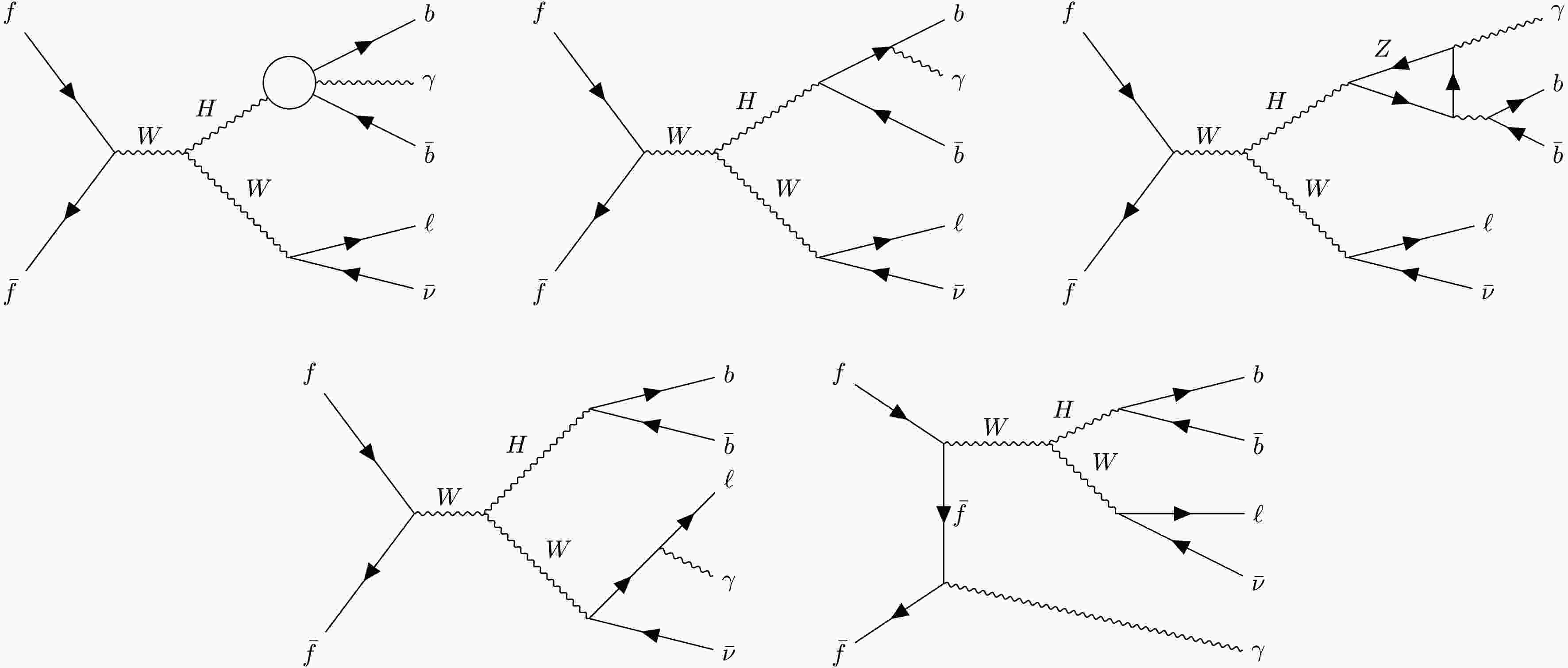
$WH\gamma$ process illustrated in Fig. 1. We focus on the topology in which the photon is radiated either from the Higgs boson sector (referred to here as the Higgs component) or from the W boson or quark lines (referred to here as the non-Higgs component). Both contributions lead to the same reconstructed final-state signature, consisting of one charged lepton, missing transverse momentum, two b-tagged jets, and one photon. We consider the leptonic decay mode$ W\to \ell\nu $ , which offers a cleaner experimental signature than the hadronic W boson decay, together with$ H \to b\bar{b} $ and$ H \to b\bar b\gamma $ final states.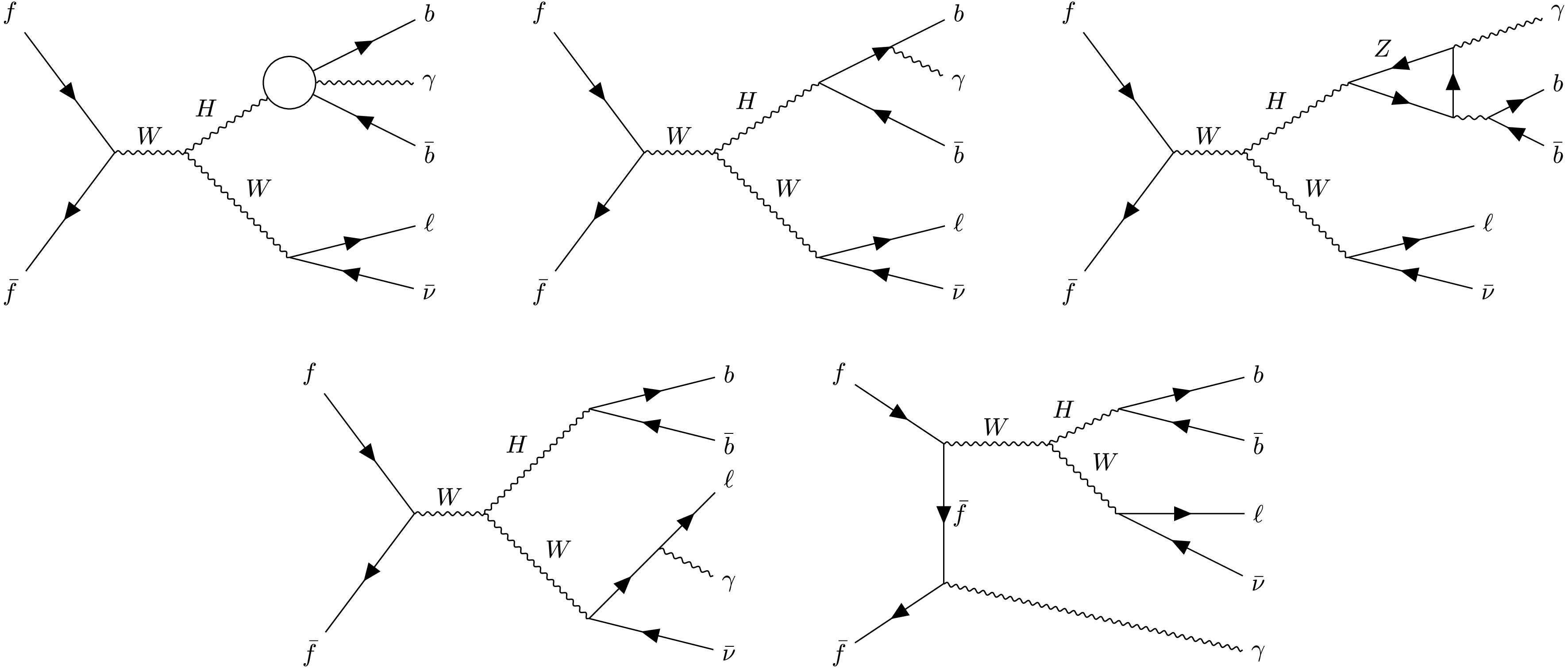
Figure 1. Feynman diagrams for the
$WH\gamma$ signal process. Top left: Higgs radiation; top center: QED process; top right:$ H\to Z\gamma $ process. Bottom left: W boson decay (leptonic); bottom right: quark radiation. We consider W boson decay and quark radiation as non-Higgs component.Our simulation framework is based on
$\mathrm{MadGraph5}\_ \mathrm{aMCNLO}$ [20] for matrix-element event generation,$\mathrm{Pythia 8.3}$ [21] for parton showering and hadronization, and$\mathrm{Delphes 3.5}$ [22] for fast detector simulation. To model the$ H\to b\bar b\gamma $ contribution, we first generate the undecayed$WH\gamma$ process and then perform the Higgs boson decay with$\mathrm{MadSpin}$ [23] using a model implemented in the Universal FeynRules Output (UFO) [24] format for the relevant effective interaction. This setup allows us to retain the characteristic dual-peak structure of the photon-energy spectrum reported in Ref. [15]. In this picture, one contribution arises from the QED process in which the photon is radiated from a final-state b-quark, while the other originates from the electroweak radiative contribution associated with Higgs boson emission. To further improve the separation between signal and background, we employ machine-learning techniques based on boosted decision trees (BDTs) implemented with the XGBoost package [25]. This multivariate strategy enhances the sensitivity to the rare$WH\gamma$ signal in the presence of sizable SM backgrounds. -
The Standard Model (SM) has been remarkably successful in describing the fundamental particles and their interactions [1]. The discovery of the Higgs boson by the ATLAS and CMS Collaborations at the CERN Large Hadron Collider (LHC) [2, 3] completed the particle content of the SM and marked a major milestone in particle physics. Nevertheless, several important questions remain unresolved, including the nature of dark matter, the origin of neutrino masses, and the baryon asymmetry of the Universe. In this context, precision studies of Higgs boson production and decay provide an important avenue for testing the SM and searching for possible effects of physics beyond it.
Numerous theoretical and experimental studies have been devoted to Higgs boson production in diboson final states [4–7]. Multiboson final states have also been explored at the LHC [8–12]. However, the specific Higgs-associated topology considered in this work, namely the
$WH\gamma$ process with leptonic W boson decay and hadronic Higgs boson decay, has remained comparatively less studied in the context addressed here [13, 14]. This channel leads to the$ \ell\nu b\bar b\gamma $ final state, with$ \ell=e,\mu $ , and provides a complementary probe of the electroweak structure of the SM. It is also sensitive to radiative Higgs effects contributing to the$ b\bar b\gamma $ final state, including the kinematic features discussed in Ref. [15]. In addition, deviations in Higgs couplings induced by beyond-SM interactions may affect such radiative contributions and alter the corresponding event distributions, making this process phenomenologically interesting for both precision studies and searches for new physics [15, 16].The LHC [17] provides an excellent environment for studying Higgs boson processes because of its high center-of-mass energy and luminosity. Although the Higgs boson has been extensively investigated in more established channels such as
$ ZZ $ and$ WW $ , the$WH\gamma$ process remains experimentally challenging because of its relatively small production rate and complex final-state composition. With the increased luminosity of Run 3 and the prospects for the High-Luminosity LHC (HL-LHC) [18], more sensitive measurements of rare associated-production channels are becoming increasingly feasible [19]. The CMS detector, with its high-performance tracking system, calorimetry, and muon chambers, is well suited to reconstructing the leptonic W boson decay, identifying two b-tagged jets from Higgs boson decay, and selecting an isolated photon in$WH\gamma$ candidate events.In this study, we investigate the
$WH\gamma$ process illustrated in Fig. 1. We focus on the topology in which the photon is radiated either from the Higgs boson sector (referred to here as the Higgs component) or from the W boson or quark lines (referred to here as the non-Higgs component). Both contributions lead to the same reconstructed final-state signature, consisting of one charged lepton, missing transverse momentum, two b-tagged jets, and one photon. We consider the leptonic decay mode$ W\to \ell\nu $ , which offers a cleaner experimental signature than the hadronic W boson decay, together with$ H \to b\bar{b} $ and$ H \to b\bar b\gamma $ final states.
Figure 1. Feynman diagrams for the
$WH\gamma$ signal process. Top left: Higgs radiation; top center: QED process; top right:$ H\to Z\gamma $ process. Bottom left: W boson decay (leptonic); bottom right: quark radiation. We consider W boson decay and quark radiation as non-Higgs component.Our simulation framework is based on
$\mathrm{MadGraph5}\_ \mathrm{aMCNLO}$ [20] for matrix-element event generation,$\mathrm{Pythia 8.3}$ [21] for parton showering and hadronization, and$\mathrm{Delphes 3.5}$ [22] for fast detector simulation. To model the$ H\to b\bar b\gamma $ contribution, we first generate the undecayed$WH\gamma$ process and then perform the Higgs boson decay with$\mathrm{MadSpin}$ [23] using a model implemented in the Universal FeynRules Output (UFO) [24] format for the relevant effective interaction. This setup allows us to retain the characteristic dual-peak structure of the photon-energy spectrum reported in Ref. [15]. In this picture, one contribution arises from the QED process in which the photon is radiated from a final-state b-quark, while the other originates from the electroweak radiative contribution associated with Higgs boson emission. To further improve the separation between signal and background, we employ machine-learning techniques based on boosted decision trees (BDTs) implemented with the XGBoost package [25]. This multivariate strategy enhances the sensitivity to the rare$WH\gamma$ signal in the presence of sizable SM backgrounds. -
The Standard Model (SM) has been remarkably successful in describing the fundamental particles and their interactions [1]. The discovery of the Higgs boson by the ATLAS and CMS Collaborations at the CERN Large Hadron Collider (LHC) [2, 3] completed the particle content of the SM and marked a major milestone in particle physics. Nevertheless, several important questions remain unresolved, including the nature of dark matter, the origin of neutrino masses, and the baryon asymmetry of the Universe. In this context, precision studies of Higgs boson production and decay provide an important avenue for testing the SM and searching for possible effects of physics beyond it.
Numerous theoretical and experimental studies have been devoted to Higgs boson production in diboson final states [4–7]. Multiboson final states have also been explored at the LHC [8–12]. However, the specific Higgs-associated topology considered in this work, namely the
$WH\gamma$ process with leptonic W boson decay and hadronic Higgs boson decay, has remained comparatively less studied in the context addressed here [13, 14]. This channel leads to the$ \ell\nu b\bar b\gamma $ final state, with$ \ell=e,\mu $ , and provides a complementary probe of the electroweak structure of the SM. It is also sensitive to radiative Higgs effects contributing to the$ b\bar b\gamma $ final state, including the kinematic features discussed in Ref. [15]. In addition, deviations in Higgs couplings induced by beyond-SM interactions may affect such radiative contributions and alter the corresponding event distributions, making this process phenomenologically interesting for both precision studies and searches for new physics [15, 16].The LHC [17] provides an excellent environment for studying Higgs boson processes because of its high center-of-mass energy and luminosity. Although the Higgs boson has been extensively investigated in more established channels such as
$ ZZ $ and$ WW $ , the$WH\gamma$ process remains experimentally challenging because of its relatively small production rate and complex final-state composition. With the increased luminosity of Run 3 and the prospects for the High-Luminosity LHC (HL-LHC) [18], more sensitive measurements of rare associated-production channels are becoming increasingly feasible [19]. The CMS detector, with its high-performance tracking system, calorimetry, and muon chambers, is well suited to reconstructing the leptonic W boson decay, identifying two b-tagged jets from Higgs boson decay, and selecting an isolated photon in$WH\gamma$ candidate events.In this study, we investigate the
$WH\gamma$ process illustrated in Fig. 1. We focus on the topology in which the photon is radiated either from the Higgs boson sector (referred to here as the Higgs component) or from the W boson or quark lines (referred to here as the non-Higgs component). Both contributions lead to the same reconstructed final-state signature, consisting of one charged lepton, missing transverse momentum, two b-tagged jets, and one photon. We consider the leptonic decay mode$ W\to \ell\nu $ , which offers a cleaner experimental signature than the hadronic W boson decay, together with$ H \to b\bar{b} $ and$ H \to b\bar b\gamma $ final states.
Figure 1. Feynman diagrams for the
$WH\gamma$ signal process. Top left: Higgs radiation; top center: QED process; top right:$ H\to Z\gamma $ process. Bottom left: W boson decay (leptonic); bottom right: quark radiation. We consider W boson decay and quark radiation as non-Higgs component.Our simulation framework is based on
$\mathrm{MadGraph5}\_ \mathrm{aMCNLO}$ [20] for matrix-element event generation,$\mathrm{Pythia 8.3}$ [21] for parton showering and hadronization, and$\mathrm{Delphes 3.5}$ [22] for fast detector simulation. To model the$ H\to b\bar b\gamma $ contribution, we first generate the undecayed$WH\gamma$ process and then perform the Higgs boson decay with$\mathrm{MadSpin}$ [23] using a model implemented in the Universal FeynRules Output (UFO) [24] format for the relevant effective interaction. This setup allows us to retain the characteristic dual-peak structure of the photon-energy spectrum reported in Ref. [15]. In this picture, one contribution arises from the QED process in which the photon is radiated from a final-state b-quark, while the other originates from the electroweak radiative contribution associated with Higgs boson emission. To further improve the separation between signal and background, we employ machine-learning techniques based on boosted decision trees (BDTs) implemented with the XGBoost package [25]. This multivariate strategy enhances the sensitivity to the rare$WH\gamma$ signal in the presence of sizable SM backgrounds. -
We classify the signal contributions into three categories according to the particle from which the photon is radiated: the Higgs boson, the W boson, or a quark.
In this study, the production processes are divided into two parts: the first is Higgs component, which is generated using a UFO model. The event generation proceeds in two steps. First, samples are produced with an undecayed Higgs boson, and
$\mathrm{MadSpin}$ is subsequently employed in conjunction with the UFO model to simulate the Higgs decay to$ {b} {\bar{b}}\gamma $ . This decay contains two photon-radiation processes. One is the standard QED process, in which the photon is radiated from a b-quark. The other consists of electroweak one-loop corrections, with electroweak radiative contributions associated with the Higgs-sector amplitude, including diagrams such as$ h\to \gamma Z^{\star} \to f\bar f\gamma $ and$ h\to \gamma \gamma^{\star} \to f\bar f\gamma $ . The photon energy distributions for both processes are shown in Fig. 2(a), following the characteristic structure discussed in Ref. [15]. The displayed range is restricted to the phenomenologically relevant energy window in which the electroweak radiative contribution is most clearly distinguishable from the QED component. The second part is non-Higgs component, for which we employ the sm model for event generation. Both Higgs component and non-Higgs component are simulated at leading order (LO) using$\mathrm{MadGraph5}\_\mathrm{aMCNLO}$ . When calculating the cross sections for both the signal and background processes, we use the default Parton Distribution Functions (PDFs) set, NNPDF23 [26], and set the factorization and renormalization scales to the physical boson mass.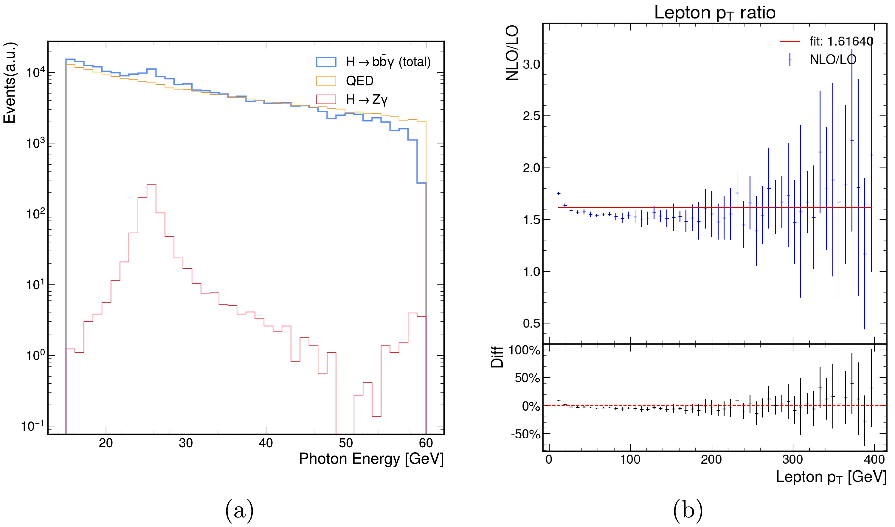
Figure 2. (color online) Left: Photon energy distribution for the Higgs component of the
$WH\gamma$ process at 13 TeV, with the QED and$ EW+\gamma $ contributions shown separately. The displayed range is restricted to highlight the region in which the electroweak contribution is most visible. Right: NLO-to-LO ratio for the lepton$ p_T $ distribution. The approximately flat behavior in the main kinematic region suggests that the higher-order correction acts primarily as an overall normalization.To estimate the impact of missing higher-order corrections, we also calculate the ratio of next-to-leading order (NLO) to LO predictions for representative kinematic observables. For example, the lepton
${p_{T}}$ distribution exhibits an approximately flat ratio, with an average K-factor of about 1.6 in the main analysis region, indicating that the dominant NLO effect is a normalization shift rather than a shape distortion.The main background processes considered in this analysis are
$ t\bar t\gamma $ ,$ tW\gamma/\bar tW\gamma $ ,$ W/Z+\gamma+{\rm{jets}} $ , and$ WW\gamma/ WZ\gamma $ . These samples are generated with$\mathrm{MadGraph5}\_ \mathrm{aMCNLO}$ , interfaced with$\mathrm{Pythia 8.3}$ for parton showering and hadronization, and processed with$\mathrm{Delphes 3.5}$ for fast detector simulation. The production cross sections used for background normalization are listed in Table 1.Process Cross Section/pb Generated Events $ p\ p \to t\bar{t}\gamma $ 2.703 $ \pm $ 0.0090745,000,000 $ p\ p \to t\bar{t} $ 214.1 $ \pm $ 0.0365,000,000 $ p\ p \to tW\gamma $ 0.315 $ \pm $ 0.000161,000,000 $ p\ p \to W/Z+\gamma+{\rm{Jets}} $ 116.2 $ \pm $ 0.35383,000,000 $ p\ p \to WW\gamma/W Z\gamma $ 0.3564 $ \pm $ 0.00092741,000,000 Table 1. Leading-order cross sections for the background processes at 13 TeV. The quoted uncertainties are the numerical integration uncertainties returned by
$\mathrm{MadGraph5}\_\mathrm{aMCNLO}$ . The full theoretical uncertainties due to missing higher-order corrections (renormalization- and factorization-scale variations) are discussed in Section IV.A right-handed coordinate system is used, with the origin at the nominal interaction point, the x-axis pointing toward the center of the LHC ring, the y-axis pointing upward, and the z-axis along the counterclockwise beam direction. The azimuthal angle ϕ is measured in the transverse plane, while the polar angle θ is defined with respect to the z-axis. The pseudorapidity is defined as
$\eta = -\ln \tan\left(\dfrac{\theta}{2}\right),$ and the separation between two objects in η-ϕ space is given by$ \Delta R = \sqrt{(\Delta\eta)^2 + (\Delta\phi)^2} $ .Electrons are reconstructed using the fast detector simulation provided by
$\mathrm{Delphes 3.5}$ . The electron tracking efficiency and efficiency parameterization depend on the transverse momentum${p_{T}}$ and pseudorapidity η of the electron. The electron momentum smearing function is based on results from the CMS Collaboration [27]. The electron isolation requirement is based on the scalar sum of the transverse momenta of all particle-flow candidates in a cone of$ \Delta R \lt 0.4 $ around the electron direction, excluding the electron itself. Muon candidates are reconstructed using efficiency corrections and momentum smearing parameterized as functions of${p_{T}}$ and η, following the same procedure as for electrons.Jets from parton showering and hadronization are reconstructed using the anti-
$ k_{t} $ clustering algorithm [28], with a distance parameter of$ R=0.4 $ and a minimum${p_{T}}$ of 20 GeV. B-jet flavour tagging is performed using$\mathrm{Delphes 3.5}$ . The b-jet tagging efficiency is parameterised as a function of jet${p_{T}}$ and η, while the light-flavour jet and c-jet mis-tagging rates are likewise parameterised as functions of jet${p_{T}}$ and η [29]. The b-tagging working point corresponds to a medium operating point, with an effective b-jet tagging efficiency of about 70% and a light-flavour mistag rate of about 1% [30]. In the fast-simulation framework, these efficiencies are applied at the reconstruction level via the$\mathrm{Delphes 3.5}$ b-tagging module.Photon candidates are reconstructed using
$\mathrm{Delphes 3.5}$ , which simulates the CMS electromagnetic calorimeter (ECAL) response. A cell granularity of$ 0.02\times 0.02 $ in$ \eta-\phi $ is assumed for both the barrel region ($ |\eta|<1.5 $ ) and the high-granularity electromagnetic calorimeter (HGCAL-ECAL) region ($ 1.5 \lt |\eta| \lt 3.0 $ ). The ECAL energy resolution is parameterised as a function of η and energy following Ref. [27, 31]. Photon isolation is defined from the scalar sum of the transverse momenta of particle-flow candidates in a cone of$ \Delta R \lt 0.4 $ around the photon direction, excluding the photon itself.To select the events of interest, a series of selection criteria is applied. To select
$WH \gamma $ signal events, we require exactly one lepton consistent with a leptonic W boson decay: either one muon with$ {p_{T}} \gt 26 \,{\text{GeV}} $ and$ |\eta|< 2.4 $ , or one electron with$ {p_{T}} \gt 30 \,{\text{GeV}} $ and$ |\eta| \lt 2.4 $ . Events are also required to have$p_{T}^\text{miss}$ greater than 30 GeV in order to suppress backgrounds without genuine missing transverse momentum and to enhance compatibility with the leptonic$ W\to \ell\nu $ topology. In addition, both$ H\to {b} {\bar{b}} \gamma $ and$ H \to {b} {\bar{b}} $ decay modes require two b-quarks, so we require events to contain at least two b-tagged jets, corresponding to the two jets from the Higgs boson decay. Since both b-jets are decay products of one Higgs boson, we require$ \Delta R_{j_1j_2} \lt 4 $ , a pseudorapidity difference between the jets of$ \Delta \eta_{j_1j_2} \lt 3.0 $ , and an azimuthal angle difference of$ \Delta \phi_{j_1j_2} \lt 2.0 $ . We also require a photon with$ {p_{T}} \gt 20 \,{\text{GeV}} $ .The cumulative event yields after successive selection requirements are summarized in Table 2, normalized to an integrated luminosity of
$ 440\; {\rm{fb}}^{-1} $ . The loose selection (denoted as ''L1'') includes the lepton, photon,$ p_{T}^\text{miss}$ , and two-b-jet requirements. Further selections, denoted as ''L2'', tighten the kinematic selection by applying$ \Delta R $ ,$ \Delta\eta $ , and$ \Delta\phi $ constraints on the jet pair. The BDT requirement and the final photon${p_{T}}$ and jet multiplicity requirements substantially suppress the leading backgrounds while retaining a meaningful fraction of the signal. Fluctuations in the predicted yields for the signal components, especially the Higgs component, reflect the limited Monte Carlo statistics, which is accounted for in the systematic uncertainty discussion in Section IV.Process L1 (basic) L2 (+ $ \Delta R $ )L2 + BDT $> $ 0.6$ +N_{\rm{jet}}=2 $ –3$ +p_T^\gamma>50 $ GeVsignal (higgs) 3.83 2.80 1.01 1.01 0.36 signal (non-higgs) 29.43 23.67 9.53 9.44 5.39 signal (total) 33.26 26.47 10.54 10.45 5.75 background 35401.59 15221.26 113.45 106.33 52.89 Total 35434.85 15247.73 123.99 116.78 58.64 Table 2. Cumulative event yields for the signal processes (Higgs and non-Higgs components) and background processes after successive selection requirements, normalized to
$ {\cal{L}}=440\; {\rm{fb}}^{-1} $ . L1 includes requirements on the lepton, photon,$ p_{T}^\text{miss}$ , and two b jets. L2 further tightens the kinematic selection by imposing constraints on$ \Delta R $ ,$ \Delta\eta $ , and$ \Delta\phi $ . The final three columns show the additional impact of$ {\rm{BDT}}>0.6 $ , the requirement$ N_{\rm{jet}}=2 $ –3, and$ p_{T}^\gamma>50 \,{\text{GeV}} $ , respectively. All yields are given by the product of the cross section, luminosity, and cumulative efficiency at each stage.The fake-photon background, arising primarily from jets misidentified as photons in QCD multijet processes, is a potentially important reducible background for this channel. A reliable estimate of the jet-to-photon fake rate would require detector-level photon-identification variables, such as the shower-shape observable
$ \sigma_{i\eta i\eta} $ and the hadronic-to-electromagnetic energy ratio$ H/E $ , or data-driven techniques based on control regions; these are beyond the scope of the present fast-simulation study. In this work, we do not attempt a quantitative estimate of the fake-photon background. Instead, we acknowledge it as a source of reducible background that should be addressed in a full experimental analysis. To mitigate the potential impact of fake photons, which are expected to be concentrated in the low-${p_{T}}$ region, we impose a tighter photon${p_{T}}$ requirement of$ p_{T}^{\gamma}>50 \,{\text{GeV}} $ in the final signal region shown in Fig. 3.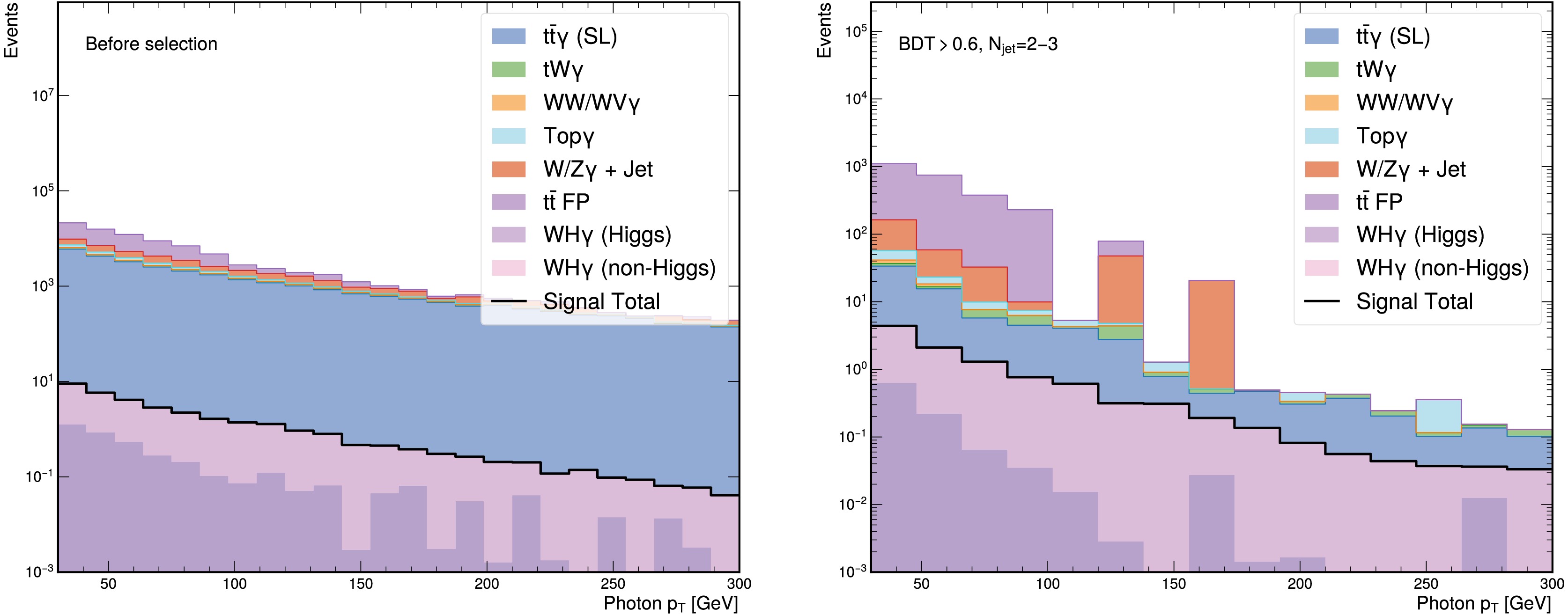
Figure 3. (color online) Photon transverse-momentum distributions before selection (left) and after selection (right), shown for an integrated luminosity of 440 fb−1. The background contributions are stacked, and the signal components are overlaid for visibility. The displayed range is restricted for plotting purposes and does not imply an additional analysis selection.
-
We classify the signal contributions into three categories according to the particle from which the photon is radiated: the Higgs boson, the W boson, or a quark.
In this study, the production processes are divided into two parts: the first is Higgs component, which is generated using a UFO model. The event generation proceeds in two steps. First, samples are produced with an undecayed Higgs boson, and
$\mathrm{MadSpin}$ is subsequently employed in conjunction with the UFO model to simulate the Higgs decay to$ {b} {\bar{b}}\gamma $ . This decay contains two photon-radiation processes. One is the standard QED process, in which the photon is radiated from a b-quark. The other consists of electroweak one-loop corrections, with electroweak radiative contributions associated with the Higgs-sector amplitude, including diagrams such as$ h\to \gamma Z^{\star} \to f\bar f\gamma $ and$ h\to \gamma \gamma^{\star} \to f\bar f\gamma $ . The photon energy distributions for both processes are shown in Fig. 2(a), following the characteristic structure discussed in Ref. [15]. The displayed range is restricted to the phenomenologically relevant energy window in which the electroweak radiative contribution is most clearly distinguishable from the QED component. The second part is non-Higgs component, for which we employ the sm model for event generation. Both Higgs component and non-Higgs component are simulated at leading order (LO) using$\mathrm{MadGraph5}\_\mathrm{aMCNLO}$ . When calculating the cross sections for both the signal and background processes, we use the default Parton Distribution Functions (PDFs) set, NNPDF23 [26], and set the factorization and renormalization scales to the physical boson mass.
Figure 2. (color online) Left: Photon energy distribution for the Higgs component of the
$WH\gamma$ process at 13 TeV, with the QED and$ EW+\gamma $ contributions shown separately. The displayed range is restricted to highlight the region in which the electroweak contribution is most visible. Right: NLO-to-LO ratio for the lepton$ p_T $ distribution. The approximately flat behavior in the main kinematic region suggests that the higher-order correction acts primarily as an overall normalization.To estimate the impact of missing higher-order corrections, we also calculate the ratio of next-to-leading order (NLO) to LO predictions for representative kinematic observables. For example, the lepton
${p_{T}}$ distribution exhibits an approximately flat ratio, with an average K-factor of about 1.6 in the main analysis region, indicating that the dominant NLO effect is a normalization shift rather than a shape distortion.The main background processes considered in this analysis are
$ t\bar t\gamma $ ,$ tW\gamma/\bar tW\gamma $ ,$ W/Z+\gamma+{\rm{jets}} $ , and$ WW\gamma/ WZ\gamma $ . These samples are generated with$\mathrm{MadGraph5}\_ \mathrm{aMCNLO}$ , interfaced with$\mathrm{Pythia 8.3}$ for parton showering and hadronization, and processed with$\mathrm{Delphes 3.5}$ for fast detector simulation. The production cross sections used for background normalization are listed in Table 1.Process Cross Section/pb Generated Events $ p\ p \to t\bar{t}\gamma $ 2.703 $ \pm $ 0.0090745,000,000 $ p\ p \to t\bar{t} $ 214.1 $ \pm $ 0.0365,000,000 $ p\ p \to tW\gamma $ 0.315 $ \pm $ 0.000161,000,000 $ p\ p \to W/Z+\gamma+{\rm{Jets}} $ 116.2 $ \pm $ 0.35383,000,000 $ p\ p \to WW\gamma/W Z\gamma $ 0.3564 $ \pm $ 0.00092741,000,000 Table 1. Leading-order cross sections for the background processes at 13 TeV. The quoted uncertainties are the numerical integration uncertainties returned by
$\mathrm{MadGraph5}\_\mathrm{aMCNLO}$ . The full theoretical uncertainties due to missing higher-order corrections (renormalization- and factorization-scale variations) are discussed in Section IV.A right-handed coordinate system is used, with the origin at the nominal interaction point, the x-axis pointing toward the center of the LHC ring, the y-axis pointing upward, and the z-axis along the counterclockwise beam direction. The azimuthal angle ϕ is measured in the transverse plane, while the polar angle θ is defined with respect to the z-axis. The pseudorapidity is defined as
$\eta = -\ln \tan\left(\dfrac{\theta}{2}\right),$ and the separation between two objects in η-ϕ space is given by$ \Delta R = \sqrt{(\Delta\eta)^2 + (\Delta\phi)^2} $ .Electrons are reconstructed using the fast detector simulation provided by
$\mathrm{Delphes 3.5}$ . The electron tracking efficiency and efficiency parameterization depend on the transverse momentum${p_{T}}$ and pseudorapidity η of the electron. The electron momentum smearing function is based on results from the CMS Collaboration [27]. The electron isolation requirement is based on the scalar sum of the transverse momenta of all particle-flow candidates in a cone of$ \Delta R \lt 0.4 $ around the electron direction, excluding the electron itself. Muon candidates are reconstructed using efficiency corrections and momentum smearing parameterized as functions of${p_{T}}$ and η, following the same procedure as for electrons.Jets from parton showering and hadronization are reconstructed using the anti-
$ k_{t} $ clustering algorithm [28], with a distance parameter of$ R=0.4 $ and a minimum${p_{T}}$ of 20 GeV. B-jet flavour tagging is performed using$\mathrm{Delphes 3.5}$ . The b-jet tagging efficiency is parameterised as a function of jet${p_{T}}$ and η, while the light-flavour jet and c-jet mis-tagging rates are likewise parameterised as functions of jet${p_{T}}$ and η [29]. The b-tagging working point corresponds to a medium operating point, with an effective b-jet tagging efficiency of about 70% and a light-flavour mistag rate of about 1% [30]. In the fast-simulation framework, these efficiencies are applied at the reconstruction level via the$\mathrm{Delphes 3.5}$ b-tagging module.Photon candidates are reconstructed using
$\mathrm{Delphes 3.5}$ , which simulates the CMS electromagnetic calorimeter (ECAL) response. A cell granularity of$ 0.02\times 0.02 $ in$ \eta-\phi $ is assumed for both the barrel region ($ |\eta|<1.5 $ ) and the high-granularity electromagnetic calorimeter (HGCAL-ECAL) region ($ 1.5 \lt |\eta| \lt 3.0 $ ). The ECAL energy resolution is parameterised as a function of η and energy following Ref. [27, 31]. Photon isolation is defined from the scalar sum of the transverse momenta of particle-flow candidates in a cone of$ \Delta R \lt 0.4 $ around the photon direction, excluding the photon itself.To select the events of interest, a series of selection criteria is applied. To select
$WH \gamma $ signal events, we require exactly one lepton consistent with a leptonic W boson decay: either one muon with$ {p_{T}} \gt 26 \,{\text{GeV}} $ and$ |\eta|< 2.4 $ , or one electron with$ {p_{T}} \gt 30 \,{\text{GeV}} $ and$ |\eta| \lt 2.4 $ . Events are also required to have$p_{T}^\text{miss}$ greater than 30 GeV in order to suppress backgrounds without genuine missing transverse momentum and to enhance compatibility with the leptonic$ W\to \ell\nu $ topology. In addition, both$ H\to {b} {\bar{b}} \gamma $ and$ H \to {b} {\bar{b}} $ decay modes require two b-quarks, so we require events to contain at least two b-tagged jets, corresponding to the two jets from the Higgs boson decay. Since both b-jets are decay products of one Higgs boson, we require$ \Delta R_{j_1j_2} \lt 4 $ , a pseudorapidity difference between the jets of$ \Delta \eta_{j_1j_2} \lt 3.0 $ , and an azimuthal angle difference of$ \Delta \phi_{j_1j_2} \lt 2.0 $ . We also require a photon with$ {p_{T}} \gt 20 \,{\text{GeV}} $ .The cumulative event yields after successive selection requirements are summarized in Table 2, normalized to an integrated luminosity of
$ 440\; {\rm{fb}}^{-1} $ . The loose selection (denoted as ''L1'') includes the lepton, photon,$ p_{T}^\text{miss}$ , and two-b-jet requirements. Further selections, denoted as ''L2'', tighten the kinematic selection by applying$ \Delta R $ ,$ \Delta\eta $ , and$ \Delta\phi $ constraints on the jet pair. The BDT requirement and the final photon${p_{T}}$ and jet multiplicity requirements substantially suppress the leading backgrounds while retaining a meaningful fraction of the signal. Fluctuations in the predicted yields for the signal components, especially the Higgs component, reflect the limited Monte Carlo statistics, which is accounted for in the systematic uncertainty discussion in Section IV.Process L1 (basic) L2 (+ $ \Delta R $ )L2 + BDT $> $ 0.6$ +N_{\rm{jet}}=2 $ –3$ +p_T^\gamma>50 $ GeVsignal (higgs) 3.83 2.80 1.01 1.01 0.36 signal (non-higgs) 29.43 23.67 9.53 9.44 5.39 signal (total) 33.26 26.47 10.54 10.45 5.75 background 35401.59 15221.26 113.45 106.33 52.89 Total 35434.85 15247.73 123.99 116.78 58.64 Table 2. Cumulative event yields for the signal processes (Higgs and non-Higgs components) and background processes after successive selection requirements, normalized to
$ {\cal{L}}=440\; {\rm{fb}}^{-1} $ . L1 includes requirements on the lepton, photon,$ p_{T}^\text{miss}$ , and two b jets. L2 further tightens the kinematic selection by imposing constraints on$ \Delta R $ ,$ \Delta\eta $ , and$ \Delta\phi $ . The final three columns show the additional impact of$ {\rm{BDT}}>0.6 $ , the requirement$ N_{\rm{jet}}=2 $ –3, and$ p_{T}^\gamma>50 \,{\text{GeV}} $ , respectively. All yields are given by the product of the cross section, luminosity, and cumulative efficiency at each stage.The fake-photon background, arising primarily from jets misidentified as photons in QCD multijet processes, is a potentially important reducible background for this channel. A reliable estimate of the jet-to-photon fake rate would require detector-level photon-identification variables, such as the shower-shape observable
$ \sigma_{i\eta i\eta} $ and the hadronic-to-electromagnetic energy ratio$ H/E $ , or data-driven techniques based on control regions; these are beyond the scope of the present fast-simulation study. In this work, we do not attempt a quantitative estimate of the fake-photon background. Instead, we acknowledge it as a source of reducible background that should be addressed in a full experimental analysis. To mitigate the potential impact of fake photons, which are expected to be concentrated in the low-${p_{T}}$ region, we impose a tighter photon${p_{T}}$ requirement of$ p_{T}^{\gamma}>50 \,{\text{GeV}} $ in the final signal region shown in Fig. 3.
Figure 3. (color online) Photon transverse-momentum distributions before selection (left) and after selection (right), shown for an integrated luminosity of 440 fb−1. The background contributions are stacked, and the signal components are overlaid for visibility. The displayed range is restricted for plotting purposes and does not imply an additional analysis selection.
-
We classify the signal contributions into three categories according to the particle from which the photon is radiated: the Higgs boson, the W boson, or a quark.
In this study, the production processes are divided into two parts: the first is Higgs component, which is generated using a UFO model. The event generation proceeds in two steps. First, samples are produced with an undecayed Higgs boson, and
$\mathrm{MadSpin}$ is subsequently employed in conjunction with the UFO model to simulate the Higgs decay to$ {b} {\bar{b}}\gamma $ . This decay contains two photon-radiation processes. One is the standard QED process, in which the photon is radiated from a b-quark. The other consists of electroweak one-loop corrections, with electroweak radiative contributions associated with the Higgs-sector amplitude, including diagrams such as$ h\to \gamma Z^{\star} \to f\bar f\gamma $ and$ h\to \gamma \gamma^{\star} \to f\bar f\gamma $ . The photon energy distributions for both processes are shown in Fig. 2(a), following the characteristic structure discussed in Ref. [15]. The displayed range is restricted to the phenomenologically relevant energy window in which the electroweak radiative contribution is most clearly distinguishable from the QED component. The second part is non-Higgs component, for which we employ the sm model for event generation. Both Higgs component and non-Higgs component are simulated at leading order (LO) using$\mathrm{MadGraph5}\_\mathrm{aMCNLO}$ . When calculating the cross sections for both the signal and background processes, we use the default Parton Distribution Functions (PDFs) set, NNPDF23 [26], and set the factorization and renormalization scales to the physical boson mass.
Figure 2. (color online) Left: Photon energy distribution for the Higgs component of the
$WH\gamma$ process at 13 TeV, with the QED and$ EW+\gamma $ contributions shown separately. The displayed range is restricted to highlight the region in which the electroweak contribution is most visible. Right: NLO-to-LO ratio for the lepton$ p_T $ distribution. The approximately flat behavior in the main kinematic region suggests that the higher-order correction acts primarily as an overall normalization.To estimate the impact of missing higher-order corrections, we also calculate the ratio of next-to-leading order (NLO) to LO predictions for representative kinematic observables. For example, the lepton
${p_{T}}$ distribution exhibits an approximately flat ratio, with an average K-factor of about 1.6 in the main analysis region, indicating that the dominant NLO effect is a normalization shift rather than a shape distortion.The main background processes considered in this analysis are
$ t\bar t\gamma $ ,$ tW\gamma/\bar tW\gamma $ ,$ W/Z+\gamma+{\rm{jets}} $ , and$ WW\gamma/ WZ\gamma $ . These samples are generated with$\mathrm{MadGraph5}\_ \mathrm{aMCNLO}$ , interfaced with$\mathrm{Pythia 8.3}$ for parton showering and hadronization, and processed with$\mathrm{Delphes 3.5}$ for fast detector simulation. The production cross sections used for background normalization are listed in Table 1.Process Cross Section/pb Generated Events $ p\ p \to t\bar{t}\gamma $ 2.703 $ \pm $ 0.0090745,000,000 $ p\ p \to t\bar{t} $ 214.1 $ \pm $ 0.0365,000,000 $ p\ p \to tW\gamma $ 0.315 $ \pm $ 0.000161,000,000 $ p\ p \to W/Z+\gamma+{\rm{Jets}} $ 116.2 $ \pm $ 0.35383,000,000 $ p\ p \to WW\gamma/W Z\gamma $ 0.3564 $ \pm $ 0.00092741,000,000 Table 1. Leading-order cross sections for the background processes at 13 TeV. The quoted uncertainties are the numerical integration uncertainties returned by
$\mathrm{MadGraph5}\_\mathrm{aMCNLO}$ . The full theoretical uncertainties due to missing higher-order corrections (renormalization- and factorization-scale variations) are discussed in Section IV.A right-handed coordinate system is used, with the origin at the nominal interaction point, the x-axis pointing toward the center of the LHC ring, the y-axis pointing upward, and the z-axis along the counterclockwise beam direction. The azimuthal angle ϕ is measured in the transverse plane, while the polar angle θ is defined with respect to the z-axis. The pseudorapidity is defined as
$\eta = -\ln \tan\left(\dfrac{\theta}{2}\right),$ and the separation between two objects in η-ϕ space is given by$ \Delta R = \sqrt{(\Delta\eta)^2 + (\Delta\phi)^2} $ .Electrons are reconstructed using the fast detector simulation provided by
$\mathrm{Delphes 3.5}$ . The electron tracking efficiency and efficiency parameterization depend on the transverse momentum${p_{T}}$ and pseudorapidity η of the electron. The electron momentum smearing function is based on results from the CMS Collaboration [27]. The electron isolation requirement is based on the scalar sum of the transverse momenta of all particle-flow candidates in a cone of$ \Delta R \lt 0.4 $ around the electron direction, excluding the electron itself. Muon candidates are reconstructed using efficiency corrections and momentum smearing parameterized as functions of${p_{T}}$ and η, following the same procedure as for electrons.Jets from parton showering and hadronization are reconstructed using the anti-
$ k_{t} $ clustering algorithm [28], with a distance parameter of$ R=0.4 $ and a minimum${p_{T}}$ of 20 GeV. B-jet flavour tagging is performed using$\mathrm{Delphes 3.5}$ . The b-jet tagging efficiency is parameterised as a function of jet${p_{T}}$ and η, while the light-flavour jet and c-jet mis-tagging rates are likewise parameterised as functions of jet${p_{T}}$ and η [29]. The b-tagging working point corresponds to a medium operating point, with an effective b-jet tagging efficiency of about 70% and a light-flavour mistag rate of about 1% [30]. In the fast-simulation framework, these efficiencies are applied at the reconstruction level via the$\mathrm{Delphes 3.5}$ b-tagging module.Photon candidates are reconstructed using
$\mathrm{Delphes 3.5}$ , which simulates the CMS electromagnetic calorimeter (ECAL) response. A cell granularity of$ 0.02\times 0.02 $ in$ \eta-\phi $ is assumed for both the barrel region ($ |\eta|<1.5 $ ) and the high-granularity electromagnetic calorimeter (HGCAL-ECAL) region ($ 1.5 \lt |\eta| \lt 3.0 $ ). The ECAL energy resolution is parameterised as a function of η and energy following Ref. [27, 31]. Photon isolation is defined from the scalar sum of the transverse momenta of particle-flow candidates in a cone of$ \Delta R \lt 0.4 $ around the photon direction, excluding the photon itself.To select the events of interest, a series of selection criteria is applied. To select
$WH \gamma $ signal events, we require exactly one lepton consistent with a leptonic W boson decay: either one muon with$ {p_{T}} \gt 26 \,{\text{GeV}} $ and$ |\eta|< 2.4 $ , or one electron with$ {p_{T}} \gt 30 \,{\text{GeV}} $ and$ |\eta| \lt 2.4 $ . Events are also required to have$p_{T}^\text{miss}$ greater than 30 GeV in order to suppress backgrounds without genuine missing transverse momentum and to enhance compatibility with the leptonic$ W\to \ell\nu $ topology. In addition, both$ H\to {b} {\bar{b}} \gamma $ and$ H \to {b} {\bar{b}} $ decay modes require two b-quarks, so we require events to contain at least two b-tagged jets, corresponding to the two jets from the Higgs boson decay. Since both b-jets are decay products of one Higgs boson, we require$ \Delta R_{j_1j_2} \lt 4 $ , a pseudorapidity difference between the jets of$ \Delta \eta_{j_1j_2} \lt 3.0 $ , and an azimuthal angle difference of$ \Delta \phi_{j_1j_2} \lt 2.0 $ . We also require a photon with$ {p_{T}} \gt 20 \,{\text{GeV}} $ .The cumulative event yields after successive selection requirements are summarized in Table 2, normalized to an integrated luminosity of
$ 440\; {\rm{fb}}^{-1} $ . The loose selection (denoted as ''L1'') includes the lepton, photon,$ p_{T}^\text{miss}$ , and two-b-jet requirements. Further selections, denoted as ''L2'', tighten the kinematic selection by applying$ \Delta R $ ,$ \Delta\eta $ , and$ \Delta\phi $ constraints on the jet pair. The BDT requirement and the final photon${p_{T}}$ and jet multiplicity requirements substantially suppress the leading backgrounds while retaining a meaningful fraction of the signal. Fluctuations in the predicted yields for the signal components, especially the Higgs component, reflect the limited Monte Carlo statistics, which is accounted for in the systematic uncertainty discussion in Section IV.Process L1 (basic) L2 (+ $ \Delta R $ )L2 + BDT $> $ 0.6$ +N_{\rm{jet}}=2 $ –3$ +p_T^\gamma>50 $ GeVsignal (higgs) 3.83 2.80 1.01 1.01 0.36 signal (non-higgs) 29.43 23.67 9.53 9.44 5.39 signal (total) 33.26 26.47 10.54 10.45 5.75 background 35401.59 15221.26 113.45 106.33 52.89 Total 35434.85 15247.73 123.99 116.78 58.64 Table 2. Cumulative event yields for the signal processes (Higgs and non-Higgs components) and background processes after successive selection requirements, normalized to
$ {\cal{L}}=440\; {\rm{fb}}^{-1} $ . L1 includes requirements on the lepton, photon,$ p_{T}^\text{miss}$ , and two b jets. L2 further tightens the kinematic selection by imposing constraints on$ \Delta R $ ,$ \Delta\eta $ , and$ \Delta\phi $ . The final three columns show the additional impact of$ {\rm{BDT}}>0.6 $ , the requirement$ N_{\rm{jet}}=2 $ –3, and$ p_{T}^\gamma>50 \,{\text{GeV}} $ , respectively. All yields are given by the product of the cross section, luminosity, and cumulative efficiency at each stage.The fake-photon background, arising primarily from jets misidentified as photons in QCD multijet processes, is a potentially important reducible background for this channel. A reliable estimate of the jet-to-photon fake rate would require detector-level photon-identification variables, such as the shower-shape observable
$ \sigma_{i\eta i\eta} $ and the hadronic-to-electromagnetic energy ratio$ H/E $ , or data-driven techniques based on control regions; these are beyond the scope of the present fast-simulation study. In this work, we do not attempt a quantitative estimate of the fake-photon background. Instead, we acknowledge it as a source of reducible background that should be addressed in a full experimental analysis. To mitigate the potential impact of fake photons, which are expected to be concentrated in the low-${p_{T}}$ region, we impose a tighter photon${p_{T}}$ requirement of$ p_{T}^{\gamma}>50 \,{\text{GeV}} $ in the final signal region shown in Fig. 3.
Figure 3. (color online) Photon transverse-momentum distributions before selection (left) and after selection (right), shown for an integrated luminosity of 440 fb−1. The background contributions are stacked, and the signal components are overlaid for visibility. The displayed range is restricted for plotting purposes and does not imply an additional analysis selection.
-
We employ a Boosted Decision Tree (BDT) [32] multivariate analysis to combine several discriminating variables into a single BDT score.
$\mathrm{XGBoost}$ is chosen for its robustness and widespread use in high-energy physics analyses.To retain sufficient information for the BDT training, a set of looser requirements is applied to the events. We require a transverse momentum of
${p_{T}^{\ell}} \gt 15 \,{\text{GeV}} $ and a pseudorapidity of$ |\eta^{\ell}| \lt 2.4 $ for both electrons and muons. At this stage, the efficiency for the signal process is approximately 5%. We select a set of kinematic variables as inputs for the BDT training. These input variables include the${p_{T}}$ , η, and ϕ of the lepton (electron or muon) and the photon. The missing transverse momentum${p_{T}^\text{miss}}$ is also included as an input variable. Jet information is incorporated into the BDT through a set of event-level observables constructed from the jet four-momentum variables (${p_{T}}$ , η, ϕ, and mass), the jet cone geometry ($ \Delta \eta $ and$ \Delta \phi $ ), and b-tagging information.For each jet variable
$ v_i $ , where i runs over all jets in the event, we compute the following aggregate quantities: the sum$ \sum_i v_i $ , the mean$ \frac{1}{n}\sum_i v_i $ , the variance$ \sum_i(v_i-\bar{v})^2 $ , the jet multiplicity n, and the leading and subleading values of$ v_i $ . For the b-tagging information, only two quantities are retained: the number of b-tagged jets and the ratio of the b-tagged jet multiplicity to the total jet multiplicity. This construction ensures a fixed number of input variables per event, regardless of jet multiplicity. The efficiencies of events for each process after preselection and the BDT cut are listed in Table 3.Process Efficiency signal(Higgs component) 1.4% signal(non-Higgs component) 7.6% $ t\bar{t}\gamma $ 12.2% $ tW\gamma/\bar{t}W\gamma $ 14.1% $ W/Z+\gamma+{\rm{Jets}} $ 5.4% $ WW\gamma/W Z\gamma $ 12.3% Table 3. Efficiency of Pre-selection for Training Samples.
For the BDT training, we use the simulated signal and background samples described above, with the corresponding generated event yields for the background processes summarized in Table 1. The signal events are assigned the label ''1'', whereas the background events are assigned the label ''0''. The training procedure is based on the
$\mathrm{XGBoost}$ package. We split the dataset into two parts: 80% of the events are used to train the model, while the remaining 20% are reserved for validation after reshuffling. We evaluate the expected significance as a function of the BDT threshold within a counting-experiment framework and choose the final signal region as$ {\rm{BDT}} \gt 0.6 $ . The feature-importance ranking shown in Fig. 4 is based on the built-in feature-importance measure of$\mathrm{XGBoost}$ and is intended only as a qualitative indication of the variables most frequently used by the classifier. Since several input observables are correlated, the ordering should not be interpreted as a unique or fully robust measure of physical relevance. The resulting BDT score distributions are shown in Fig. 5.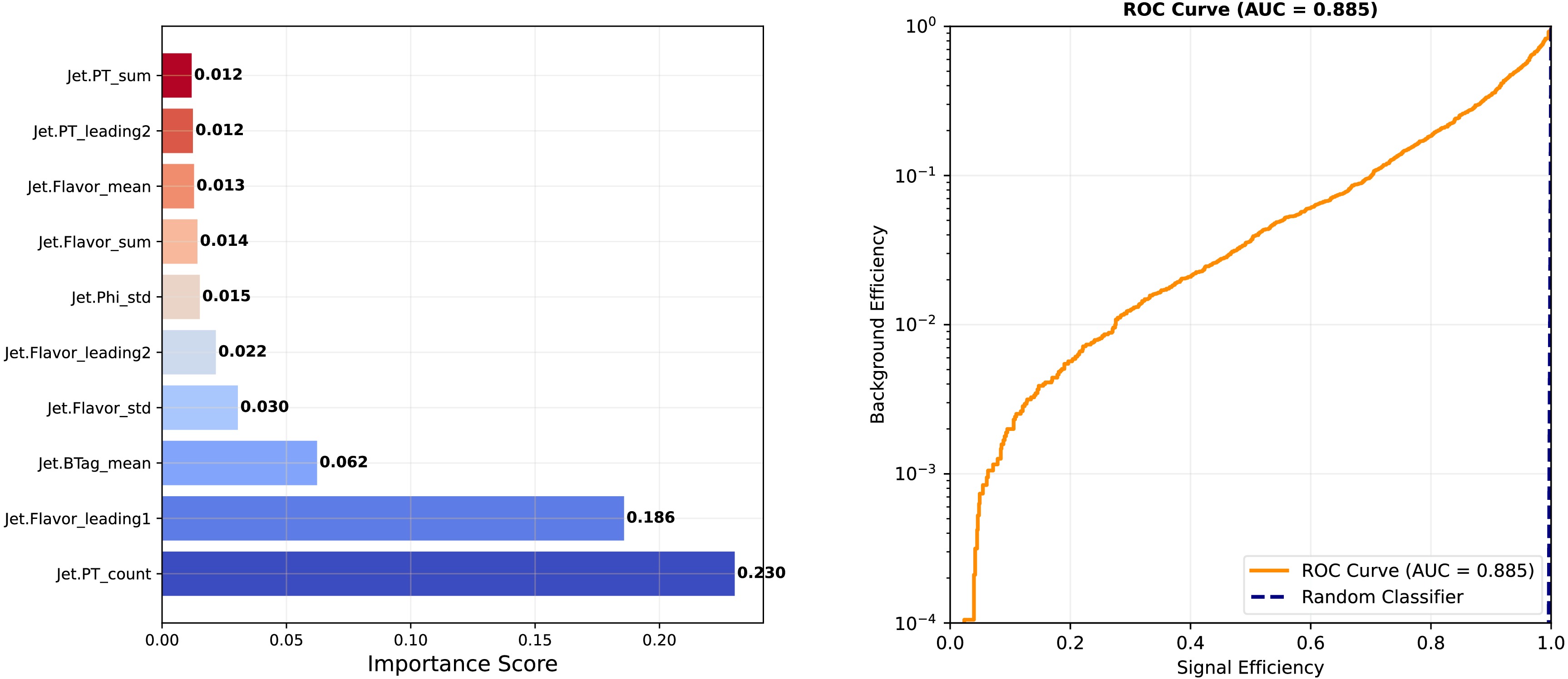
Figure 4. (color online) Left: Feature importance for BDT training (top 10 variables). Right: ROC curve for BDT training (AUC = 0.790).
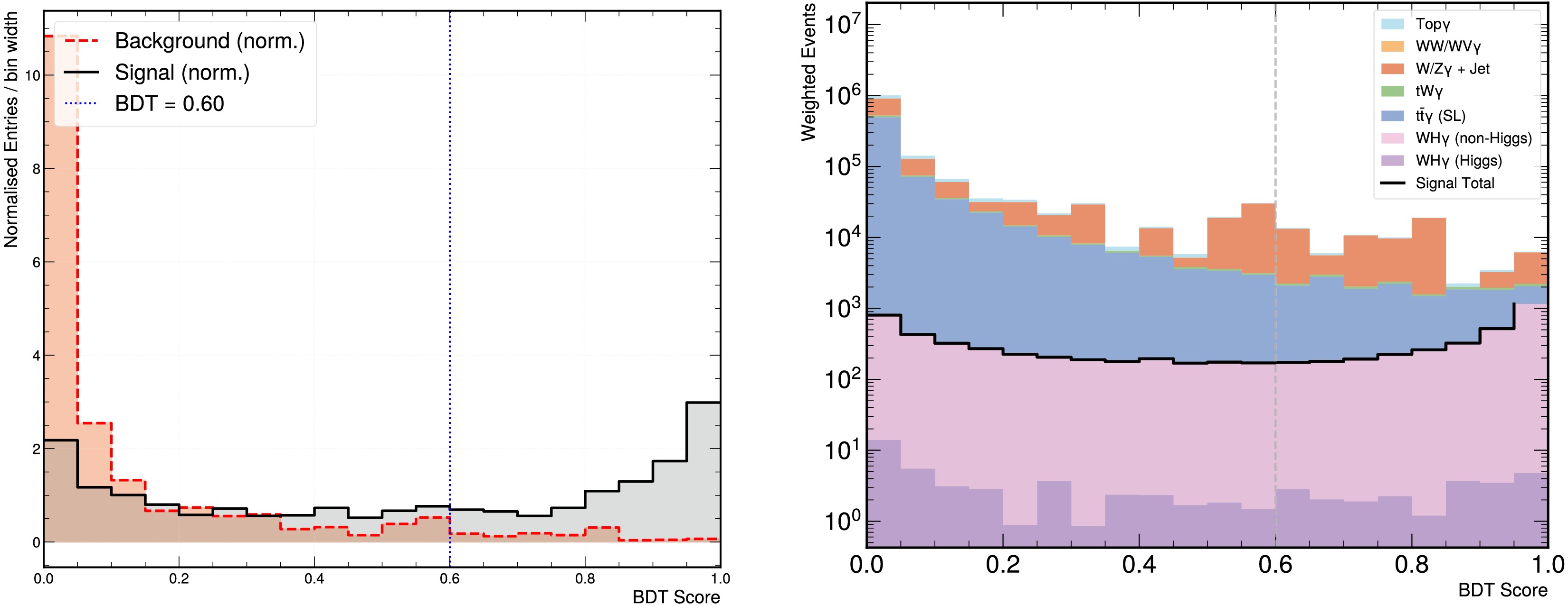
Figure 5. (color online) Left: Normalized BDT score distributions for the signal and background. Right: Expected weighted event distribution, with stacked backgrounds and overlaid
$WH\gamma$ signal components. The vertical line indicates the final requirement,$ {\rm{BDT}}>0.6 $ .The transverse W-boson mass is constructed from the lepton and missing transverse momentum as
$ m_{T} ^{W} = \sqrt{2\ p_{T}^{\ell} \cdot p_{T}^\text{miss} \cdot(1-\cos\Delta \varphi)} $ , where$ \Delta \varphi $ is the angle between the lepton and the missing transverse momentum in the transverse plane. As illustrated in Fig. 6, applying the BDT selection suppresses a large fraction of the background while retaining part of the signal contribution. This behavior is consistent with the separation observed in the BDT-score distribution.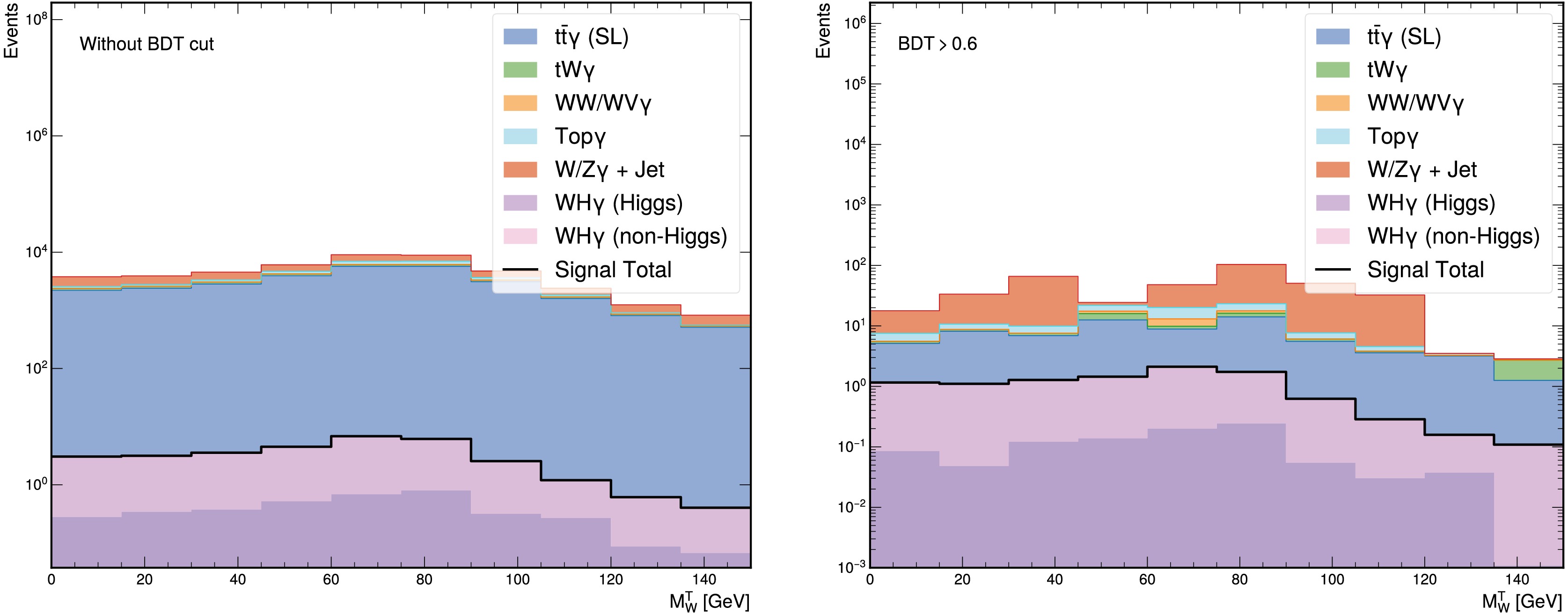
Figure 6. (color online) Left: Transverse W-boson mass distribution without the BDT cut. Right: Transverse W-boson mass distribution with the BDT cut.
The invariant mass
$ m_{bb} $ is reconstructed from the two leading b-tagged jets in the event by combining their four-momenta. Figure 7 shows the$ m_{bb} $ distribution after application of the BDT cut for events with 2 or 3 jets. The non-Higgs component exhibits a peak around 125 GeV, consistent with the Higgs boson mass, as the two b-jets originate from Higgs boson decay. For the Higgs component, the reconstructed$ m_{bb} $ distribution peaks below 125 GeV because$ m_{bb} $ is constructed only from the two b-tagged jets, while the photon in the radiative$ b\bar b\gamma $ topology carries part of the Higgs boson energy.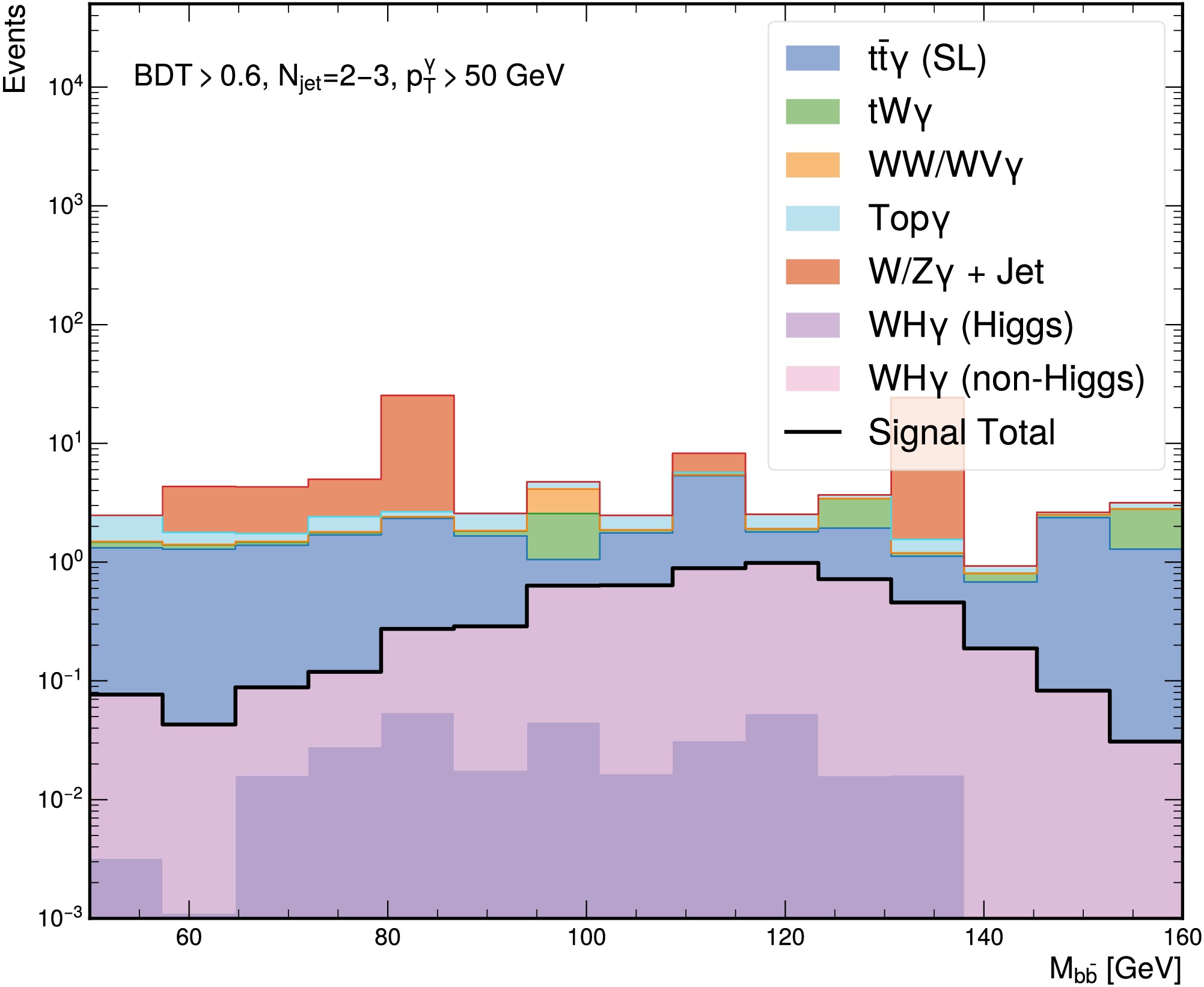
Figure 7. (color online) Invariant-mass (
$ m_{bb} $ ) distribution after the final BDT requirement for events with two or three jets and$p_{T}^\gamma>50 \,{\text{GeV}} $ . -
We employ a Boosted Decision Tree (BDT) [32] multivariate analysis to combine several discriminating variables into a single BDT score.
$\mathrm{XGBoost}$ is chosen for its robustness and widespread use in high-energy physics analyses.To retain sufficient information for the BDT training, a set of looser requirements is applied to the events. We require a transverse momentum of
${p_{T}^{\ell}} \gt 15 \,{\text{GeV}} $ and a pseudorapidity of$ |\eta^{\ell}| \lt 2.4 $ for both electrons and muons. At this stage, the efficiency for the signal process is approximately 5%. We select a set of kinematic variables as inputs for the BDT training. These input variables include the${p_{T}}$ , η, and ϕ of the lepton (electron or muon) and the photon. The missing transverse momentum${p_{T}^\text{miss}}$ is also included as an input variable. Jet information is incorporated into the BDT through a set of event-level observables constructed from the jet four-momentum variables (${p_{T}}$ , η, ϕ, and mass), the jet cone geometry ($ \Delta \eta $ and$ \Delta \phi $ ), and b-tagging information.For each jet variable
$ v_i $ , where i runs over all jets in the event, we compute the following aggregate quantities: the sum$ \sum_i v_i $ , the mean$ \frac{1}{n}\sum_i v_i $ , the variance$ \sum_i(v_i-\bar{v})^2 $ , the jet multiplicity n, and the leading and subleading values of$ v_i $ . For the b-tagging information, only two quantities are retained: the number of b-tagged jets and the ratio of the b-tagged jet multiplicity to the total jet multiplicity. This construction ensures a fixed number of input variables per event, regardless of jet multiplicity. The efficiencies of events for each process after preselection and the BDT cut are listed in Table 3.Process Efficiency signal(Higgs component) 1.4% signal(non-Higgs component) 7.6% $ t\bar{t}\gamma $ 12.2% $ tW\gamma/\bar{t}W\gamma $ 14.1% $ W/Z+\gamma+{\rm{Jets}} $ 5.4% $ WW\gamma/W Z\gamma $ 12.3% Table 3. Efficiency of Pre-selection for Training Samples.
For the BDT training, we use the simulated signal and background samples described above, with the corresponding generated event yields for the background processes summarized in Table 1. The signal events are assigned the label ''1'', whereas the background events are assigned the label ''0''. The training procedure is based on the
$\mathrm{XGBoost}$ package. We split the dataset into two parts: 80% of the events are used to train the model, while the remaining 20% are reserved for validation after reshuffling. We evaluate the expected significance as a function of the BDT threshold within a counting-experiment framework and choose the final signal region as$ {\rm{BDT}} \gt 0.6 $ . The feature-importance ranking shown in Fig. 4 is based on the built-in feature-importance measure of$\mathrm{XGBoost}$ and is intended only as a qualitative indication of the variables most frequently used by the classifier. Since several input observables are correlated, the ordering should not be interpreted as a unique or fully robust measure of physical relevance. The resulting BDT score distributions are shown in Fig. 5.
Figure 4. (color online) Left: Feature importance for BDT training (top 10 variables). Right: ROC curve for BDT training (AUC = 0.790).
Figure 5. (color online) Left: Normalized BDT score distributions for the signal and background. Right: Expected weighted event distribution, with stacked backgrounds and overlaid
$WH\gamma$ signal components. The vertical line indicates the final requirement,$ {\rm{BDT}}>0.6 $ .The transverse W-boson mass is constructed from the lepton and missing transverse momentum as
$ m_{T} ^{W} = \sqrt{2\ p_{T}^{\ell} \cdot p_{T}^\text{miss} \cdot(1-\cos\Delta \varphi)} $ , where$ \Delta \varphi $ is the angle between the lepton and the missing transverse momentum in the transverse plane. As illustrated in Fig. 6, applying the BDT selection suppresses a large fraction of the background while retaining part of the signal contribution. This behavior is consistent with the separation observed in the BDT-score distribution.
Figure 6. (color online) Left: Transverse W-boson mass distribution without the BDT cut. Right: Transverse W-boson mass distribution with the BDT cut.
The invariant mass
$ m_{bb} $ is reconstructed from the two leading b-tagged jets in the event by combining their four-momenta. Figure 7 shows the$ m_{bb} $ distribution after application of the BDT cut for events with 2 or 3 jets. The non-Higgs component exhibits a peak around 125 GeV, consistent with the Higgs boson mass, as the two b-jets originate from Higgs boson decay. For the Higgs component, the reconstructed$ m_{bb} $ distribution peaks below 125 GeV because$ m_{bb} $ is constructed only from the two b-tagged jets, while the photon in the radiative$ b\bar b\gamma $ topology carries part of the Higgs boson energy.
Figure 7. (color online) Invariant-mass (
$ m_{bb} $ ) distribution after the final BDT requirement for events with two or three jets and$p_{T}^\gamma>50 \,{\text{GeV}} $ . -
We employ a Boosted Decision Tree (BDT) [32] multivariate analysis to combine several discriminating variables into a single BDT score.
$\mathrm{XGBoost}$ is chosen for its robustness and widespread use in high-energy physics analyses.To retain sufficient information for the BDT training, a set of looser requirements is applied to the events. We require a transverse momentum of
${p_{T}^{\ell}} \gt 15 \,{\text{GeV}} $ and a pseudorapidity of$ |\eta^{\ell}| \lt 2.4 $ for both electrons and muons. At this stage, the efficiency for the signal process is approximately 5%. We select a set of kinematic variables as inputs for the BDT training. These input variables include the${p_{T}}$ , η, and ϕ of the lepton (electron or muon) and the photon. The missing transverse momentum${p_{T}^\text{miss}}$ is also included as an input variable. Jet information is incorporated into the BDT through a set of event-level observables constructed from the jet four-momentum variables (${p_{T}}$ , η, ϕ, and mass), the jet cone geometry ($ \Delta \eta $ and$ \Delta \phi $ ), and b-tagging information.For each jet variable
$ v_i $ , where i runs over all jets in the event, we compute the following aggregate quantities: the sum$ \sum_i v_i $ , the mean$ \frac{1}{n}\sum_i v_i $ , the variance$ \sum_i(v_i-\bar{v})^2 $ , the jet multiplicity n, and the leading and subleading values of$ v_i $ . For the b-tagging information, only two quantities are retained: the number of b-tagged jets and the ratio of the b-tagged jet multiplicity to the total jet multiplicity. This construction ensures a fixed number of input variables per event, regardless of jet multiplicity. The efficiencies of events for each process after preselection and the BDT cut are listed in Table 3.Process Efficiency signal(Higgs component) 1.4% signal(non-Higgs component) 7.6% $ t\bar{t}\gamma $ 12.2% $ tW\gamma/\bar{t}W\gamma $ 14.1% $ W/Z+\gamma+{\rm{Jets}} $ 5.4% $ WW\gamma/W Z\gamma $ 12.3% Table 3. Efficiency of Pre-selection for Training Samples.
For the BDT training, we use the simulated signal and background samples described above, with the corresponding generated event yields for the background processes summarized in Table 1. The signal events are assigned the label ''1'', whereas the background events are assigned the label ''0''. The training procedure is based on the
$\mathrm{XGBoost}$ package. We split the dataset into two parts: 80% of the events are used to train the model, while the remaining 20% are reserved for validation after reshuffling. We evaluate the expected significance as a function of the BDT threshold within a counting-experiment framework and choose the final signal region as$ {\rm{BDT}} \gt 0.6 $ . The feature-importance ranking shown in Fig. 4 is based on the built-in feature-importance measure of$\mathrm{XGBoost}$ and is intended only as a qualitative indication of the variables most frequently used by the classifier. Since several input observables are correlated, the ordering should not be interpreted as a unique or fully robust measure of physical relevance. The resulting BDT score distributions are shown in Fig. 5.
Figure 4. (color online) Left: Feature importance for BDT training (top 10 variables). Right: ROC curve for BDT training (AUC = 0.790).
Figure 5. (color online) Left: Normalized BDT score distributions for the signal and background. Right: Expected weighted event distribution, with stacked backgrounds and overlaid
$WH\gamma$ signal components. The vertical line indicates the final requirement,$ {\rm{BDT}}>0.6 $ .The transverse W-boson mass is constructed from the lepton and missing transverse momentum as
$ m_{T} ^{W} = \sqrt{2\ p_{T}^{\ell} \cdot p_{T}^\text{miss} \cdot(1-\cos\Delta \varphi)} $ , where$ \Delta \varphi $ is the angle between the lepton and the missing transverse momentum in the transverse plane. As illustrated in Fig. 6, applying the BDT selection suppresses a large fraction of the background while retaining part of the signal contribution. This behavior is consistent with the separation observed in the BDT-score distribution.
Figure 6. (color online) Left: Transverse W-boson mass distribution without the BDT cut. Right: Transverse W-boson mass distribution with the BDT cut.
The invariant mass
$ m_{bb} $ is reconstructed from the two leading b-tagged jets in the event by combining their four-momenta. Figure 7 shows the$ m_{bb} $ distribution after application of the BDT cut for events with 2 or 3 jets. The non-Higgs component exhibits a peak around 125 GeV, consistent with the Higgs boson mass, as the two b-jets originate from Higgs boson decay. For the Higgs component, the reconstructed$ m_{bb} $ distribution peaks below 125 GeV because$ m_{bb} $ is constructed only from the two b-tagged jets, while the photon in the radiative$ b\bar b\gamma $ topology carries part of the Higgs boson energy.
Figure 7. (color online) Invariant-mass (
$ m_{bb} $ ) distribution after the final BDT requirement for events with two or three jets and$p_{T}^\gamma>50 \,{\text{GeV}} $ . -
The expected sensitivity is affected not only by the finite event yields but also by theoretical, experimental, and Monte Carlo statistical uncertainties. Because the present work is a phenomenological fast-simulation study, we do not attempt to construct a full experimental nuisance-parameter model. Instead, we adopt an effective background-uncertainty treatment to estimate the impact of the dominant uncertainty sources on the final counting sensitivity.
Theoretical normalization uncertainties arise primarily from the use of leading-order event generation and from missing higher-order QCD and electroweak corrections. Their impact is estimated through renormalization- and factorization-scale variations, in which the two scales are varied independently by factors of 0.5, 1, and 2 around the nominal value using the standard seven-point prescription. The envelope of the resulting cross-section variations is taken as a process-dependent theory uncertainty. This uncertainty is treated as a normalization uncertainty in the final background estimate.
Experimental uncertainties relevant to this final state include the integrated luminosity; lepton reconstruction and trigger efficiencies; photon reconstruction and isolation; b-tagging; jet energy scale and resolution; and missing-transverse-momentum modeling. The b-tagging and photon-related uncertainties are particularly important because the final state requires at least two b-tagged jets and one isolated photon. We assign representative uncertainties to these sources following CMS performance and HL-LHC projection studies [30, 33–35]. We adopt the S2 uncertainty-scaling scenario described in Ref. [34], in which theory uncertainties are scaled by a factor of 1/2 relative to Run 2; experimental uncertainties of statistical origin are scaled as
$ 1/\sqrt{k_{{\cal{L}}}} $ or$ \max(c,1/\sqrt{k_{{\cal{L}}}}) $ , where$ k_{{\cal{L}}} $ is the luminosity scaling factor; the luminosity uncertainty is scaled by 0.6; and the b-tagging uncertainty is kept unchanged.The dominant uncertainty components entering the effective
$ \delta_B $ at$ 440\; {\rm{fb}}^{-1} $ are as follows:● Theory normalization uncertainty (from scale variations and missing higher-order terms): 5%, conservatively increased by a factor of two for leading-order modeling, following the S2 prescription [34];
● b-tagging efficiency and mistag rate: 5%, unchanged from Run 2, following the S2 prescription [30];
● Photon identification, efficiency, and energy scale: a combined 2.5% [33, 34];
● Lepton reconstruction and trigger efficiencies: 1.5% [33];
● Jet energy scale and resolution, and
$E_T^ {\rm{miss}}$ modelling: 3% [35];● Integrated luminosity: 1.5%, following the S2 prescription [34];
● Finite MC statistics: evaluated separately for each background process using the weighted event variance after the final selection.
For the signal processes, particularly Higgs component, for which the expected yield is below one event at
$ 440\; {\rm{fb}}^{-1} $ , the finite MC sample size introduces a non-negligible uncertainty in the predicted event yield. This statistical component is propagated through the weighted event variance into the total uncertainty, as described below.For a background process i with yield
$ B_i $ and relative uncertainty$ \delta_i $ , the uncertainty in the total background yield is approximated by$ \Delta B = \sqrt{\sum\limits_i (\delta_i B_i)^2 + \Delta B_{{\rm{MC}}}^2}, $
(1) where
$ \Delta B_{{\rm{MC}}} $ denotes the statistical uncertainty arising from the finite MC sample size. The effective relative background uncertainty is then defined as$ \delta_B = \frac{\Delta B}{B}, \qquad B=\sum\limits_i B_i . $
(2) Combining all sources in quadrature, the effective background uncertainty after the final selection is approximately 8%. We therefore use
$ \delta_B$ =8% as a benchmark value in the final counting-experiment estimate. This value should be interpreted as an approximate effective uncertainty rather than as a complete experimental nuisance-parameter model. We note that the quoted values are approximate estimates suitable for a fast-simulation phenomenological study; a full experimental analysis would require a more detailed treatment, including nuisance-parameter correlations, profile-likelihood fits, and dedicated control-region measurements. The 8% benchmark is intended to illustrate the qualitative impact of realistic systematic uncertainties on the projected sensitivity.The significance, including the effective background uncertainty, is estimated as
$ Z_{{\rm{syst}}}=\frac{S}{\sqrt{B+(\delta_B B)^2}}, $
(3) where S and B denote the signal and background yields after the final selection.
We take
$ 440\; {\rm{fb}}^{-1} $ as the reference integrated luminosity for the combined LHC Run-2 and Run-3 dataset and also consider the HL-LHC scenario with$ 3000\; {\rm{fb}}^{-1} $ . The statistical significance is evaluated using$ Z_{{\rm{stat}}}=S/\sqrt{B} $ . After imposing the final selection requirements$ {\rm{BDT}}>0.6 $ ,$ p_{T}^\gamma>50 \,{\text{GeV}} $ , and the mass window$ m_{bb}\in [70, 150] \,{\text{GeV}} $ , the expected event yields and significances are summarized in Table 4.(a) 440 fb−1 Signal S B $ Z_{\text{stat}} $ $ Z_{\text{syst}} $ $WH\gamma$ (Higgs component)0.23 16.2 0.06 0.05 $WH\gamma$ (non-Higgs component)2.30 16.2 0.57 0.54 $WH\gamma$ sum2.53 16.2 0.63 0.60 (b) 3000 fb−1 Signal S B $Z_{\text{stat}}$ $Z_{\text{syst}}$ $WH\gamma$ (Higgs component)1.54 110 0.15 0.11 $WH\gamma$ (non-Higgs component)15.7 110 1.49 1.14 $WH\gamma$ sum17.2 110 1.64 1.26 Table 4. Expected event yields and significances at 13 TeV in the window
$ m_{bb}\in[70, 150] \,{\text{GeV}} $ after imposing$ {{\rm{BDT}}}>0.6 $ . The results are presented for integrated luminosities of$ 440\; {\rm{fb}}^{-1} $ and$ 3000\; {\rm{fb}}^{-1} $ . For the HL-LHC case, the event yields are obtained by linearly scaling those at$ 440\; {\rm{fb}}^{-1} $ with luminosity. The systematic significance is evaluated using an effective background uncertainty of$ \delta_B= $ 8%.The results show that the
$WH\gamma$ non-Higgs component makes the larger contribution after the final selection. At$ 440\; {\rm{fb}}^{-1} $ , its statistical significance is approximately one order of magnitude larger than that of the Higgs component. The combined$WH\gamma$ statistical significance is$ 0.63\sigma $ at$ 440\; {\rm{fb}}^{-1} $ and$ 1.64\sigma $ at$ 3000\; {\rm{fb}}^{-1} $ . After including the benchmark effective background uncertainty, these values are reduced to$ 0.60\sigma $ and$ 1.26\sigma $ , respectively. -
The expected sensitivity is affected not only by the finite event yields but also by theoretical, experimental, and Monte Carlo statistical uncertainties. Because the present work is a phenomenological fast-simulation study, we do not attempt to construct a full experimental nuisance-parameter model. Instead, we adopt an effective background-uncertainty treatment to estimate the impact of the dominant uncertainty sources on the final counting sensitivity.
Theoretical normalization uncertainties arise primarily from the use of leading-order event generation and from missing higher-order QCD and electroweak corrections. Their impact is estimated through renormalization- and factorization-scale variations, in which the two scales are varied independently by factors of 0.5, 1, and 2 around the nominal value using the standard seven-point prescription. The envelope of the resulting cross-section variations is taken as a process-dependent theory uncertainty. This uncertainty is treated as a normalization uncertainty in the final background estimate.
Experimental uncertainties relevant to this final state include the integrated luminosity; lepton reconstruction and trigger efficiencies; photon reconstruction and isolation; b-tagging; jet energy scale and resolution; and missing-transverse-momentum modeling. The b-tagging and photon-related uncertainties are particularly important because the final state requires at least two b-tagged jets and one isolated photon. We assign representative uncertainties to these sources following CMS performance and HL-LHC projection studies [30, 33–35]. We adopt the S2 uncertainty-scaling scenario described in Ref. [34], in which theory uncertainties are scaled by a factor of 1/2 relative to Run 2; experimental uncertainties of statistical origin are scaled as
$ 1/\sqrt{k_{{\cal{L}}}} $ or$ \max(c,1/\sqrt{k_{{\cal{L}}}}) $ , where$ k_{{\cal{L}}} $ is the luminosity scaling factor; the luminosity uncertainty is scaled by 0.6; and the b-tagging uncertainty is kept unchanged.The dominant uncertainty components entering the effective
$ \delta_B $ at$ 440\; {\rm{fb}}^{-1} $ are as follows:● Theory normalization uncertainty (from scale variations and missing higher-order terms): 5%, conservatively increased by a factor of two for leading-order modeling, following the S2 prescription [34];
● b-tagging efficiency and mistag rate: 5%, unchanged from Run 2, following the S2 prescription [30];
● Photon identification, efficiency, and energy scale: a combined 2.5% [33, 34];
● Lepton reconstruction and trigger efficiencies: 1.5% [33];
● Jet energy scale and resolution, and
$E_T^ {\rm{miss}}$ modelling: 3% [35];● Integrated luminosity: 1.5%, following the S2 prescription [34];
● Finite MC statistics: evaluated separately for each background process using the weighted event variance after the final selection.
For the signal processes, particularly Higgs component, for which the expected yield is below one event at
$ 440\; {\rm{fb}}^{-1} $ , the finite MC sample size introduces a non-negligible uncertainty in the predicted event yield. This statistical component is propagated through the weighted event variance into the total uncertainty, as described below.For a background process i with yield
$ B_i $ and relative uncertainty$ \delta_i $ , the uncertainty in the total background yield is approximated by$ \Delta B = \sqrt{\sum\limits_i (\delta_i B_i)^2 + \Delta B_{{\rm{MC}}}^2}, $
(1) where
$ \Delta B_{{\rm{MC}}} $ denotes the statistical uncertainty arising from the finite MC sample size. The effective relative background uncertainty is then defined as$ \delta_B = \frac{\Delta B}{B}, \qquad B=\sum\limits_i B_i . $
(2) Combining all sources in quadrature, the effective background uncertainty after the final selection is approximately 8%. We therefore use
$ \delta_B$ =8% as a benchmark value in the final counting-experiment estimate. This value should be interpreted as an approximate effective uncertainty rather than as a complete experimental nuisance-parameter model. We note that the quoted values are approximate estimates suitable for a fast-simulation phenomenological study; a full experimental analysis would require a more detailed treatment, including nuisance-parameter correlations, profile-likelihood fits, and dedicated control-region measurements. The 8% benchmark is intended to illustrate the qualitative impact of realistic systematic uncertainties on the projected sensitivity.The significance, including the effective background uncertainty, is estimated as
$ Z_{{\rm{syst}}}=\frac{S}{\sqrt{B+(\delta_B B)^2}}, $
(3) where S and B denote the signal and background yields after the final selection.
We take
$ 440\; {\rm{fb}}^{-1} $ as the reference integrated luminosity for the combined LHC Run-2 and Run-3 dataset and also consider the HL-LHC scenario with$ 3000\; {\rm{fb}}^{-1} $ . The statistical significance is evaluated using$ Z_{{\rm{stat}}}=S/\sqrt{B} $ . After imposing the final selection requirements$ {\rm{BDT}}>0.6 $ ,$ p_{T}^\gamma>50 \,{\text{GeV}} $ , and the mass window$ m_{bb}\in [70, 150] \,{\text{GeV}} $ , the expected event yields and significances are summarized in Table 4.(a) 440 fb−1 Signal S B $ Z_{\text{stat}} $ $ Z_{\text{syst}} $ $WH\gamma$ (Higgs component)0.23 16.2 0.06 0.05 $WH\gamma$ (non-Higgs component)2.30 16.2 0.57 0.54 $WH\gamma$ sum2.53 16.2 0.63 0.60 (b) 3000 fb−1 Signal S B $Z_{\text{stat}}$ $Z_{\text{syst}}$ $WH\gamma$ (Higgs component)1.54 110 0.15 0.11 $WH\gamma$ (non-Higgs component)15.7 110 1.49 1.14 $WH\gamma$ sum17.2 110 1.64 1.26 Table 4. Expected event yields and significances at 13 TeV in the window
$ m_{bb}\in[70, 150] \,{\text{GeV}} $ after imposing$ {{\rm{BDT}}}>0.6 $ . The results are presented for integrated luminosities of$ 440\; {\rm{fb}}^{-1} $ and$ 3000\; {\rm{fb}}^{-1} $ . For the HL-LHC case, the event yields are obtained by linearly scaling those at$ 440\; {\rm{fb}}^{-1} $ with luminosity. The systematic significance is evaluated using an effective background uncertainty of$ \delta_B= $ 8%.The results show that the
$WH\gamma$ non-Higgs component makes the larger contribution after the final selection. At$ 440\; {\rm{fb}}^{-1} $ , its statistical significance is approximately one order of magnitude larger than that of the Higgs component. The combined$WH\gamma$ statistical significance is$ 0.63\sigma $ at$ 440\; {\rm{fb}}^{-1} $ and$ 1.64\sigma $ at$ 3000\; {\rm{fb}}^{-1} $ . After including the benchmark effective background uncertainty, these values are reduced to$ 0.60\sigma $ and$ 1.26\sigma $ , respectively. -
The expected sensitivity is affected not only by the finite event yields but also by theoretical, experimental, and Monte Carlo statistical uncertainties. Because the present work is a phenomenological fast-simulation study, we do not attempt to construct a full experimental nuisance-parameter model. Instead, we adopt an effective background-uncertainty treatment to estimate the impact of the dominant uncertainty sources on the final counting sensitivity.
Theoretical normalization uncertainties arise primarily from the use of leading-order event generation and from missing higher-order QCD and electroweak corrections. Their impact is estimated through renormalization- and factorization-scale variations, in which the two scales are varied independently by factors of 0.5, 1, and 2 around the nominal value using the standard seven-point prescription. The envelope of the resulting cross-section variations is taken as a process-dependent theory uncertainty. This uncertainty is treated as a normalization uncertainty in the final background estimate.
Experimental uncertainties relevant to this final state include the integrated luminosity; lepton reconstruction and trigger efficiencies; photon reconstruction and isolation; b-tagging; jet energy scale and resolution; and missing-transverse-momentum modeling. The b-tagging and photon-related uncertainties are particularly important because the final state requires at least two b-tagged jets and one isolated photon. We assign representative uncertainties to these sources following CMS performance and HL-LHC projection studies [30, 33–35]. We adopt the S2 uncertainty-scaling scenario described in Ref. [34], in which theory uncertainties are scaled by a factor of 1/2 relative to Run 2; experimental uncertainties of statistical origin are scaled as
$ 1/\sqrt{k_{{\cal{L}}}} $ or$ \max(c,1/\sqrt{k_{{\cal{L}}}}) $ , where$ k_{{\cal{L}}} $ is the luminosity scaling factor; the luminosity uncertainty is scaled by 0.6; and the b-tagging uncertainty is kept unchanged.The dominant uncertainty components entering the effective
$ \delta_B $ at$ 440\; {\rm{fb}}^{-1} $ are as follows:● Theory normalization uncertainty (from scale variations and missing higher-order terms): 5%, conservatively increased by a factor of two for leading-order modeling, following the S2 prescription [34];
● b-tagging efficiency and mistag rate: 5%, unchanged from Run 2, following the S2 prescription [30];
● Photon identification, efficiency, and energy scale: a combined 2.5% [33, 34];
● Lepton reconstruction and trigger efficiencies: 1.5% [33];
● Jet energy scale and resolution, and
$E_T^ {\rm{miss}}$ modelling: 3% [35];● Integrated luminosity: 1.5%, following the S2 prescription [34];
● Finite MC statistics: evaluated separately for each background process using the weighted event variance after the final selection.
For the signal processes, particularly Higgs component, for which the expected yield is below one event at
$ 440\; {\rm{fb}}^{-1} $ , the finite MC sample size introduces a non-negligible uncertainty in the predicted event yield. This statistical component is propagated through the weighted event variance into the total uncertainty, as described below.For a background process i with yield
$ B_i $ and relative uncertainty$ \delta_i $ , the uncertainty in the total background yield is approximated by$ \Delta B = \sqrt{\sum\limits_i (\delta_i B_i)^2 + \Delta B_{{\rm{MC}}}^2}, $
(1) where
$ \Delta B_{{\rm{MC}}} $ denotes the statistical uncertainty arising from the finite MC sample size. The effective relative background uncertainty is then defined as$ \delta_B = \frac{\Delta B}{B}, \qquad B=\sum\limits_i B_i . $
(2) Combining all sources in quadrature, the effective background uncertainty after the final selection is approximately 8%. We therefore use
$ \delta_B$ =8% as a benchmark value in the final counting-experiment estimate. This value should be interpreted as an approximate effective uncertainty rather than as a complete experimental nuisance-parameter model. We note that the quoted values are approximate estimates suitable for a fast-simulation phenomenological study; a full experimental analysis would require a more detailed treatment, including nuisance-parameter correlations, profile-likelihood fits, and dedicated control-region measurements. The 8% benchmark is intended to illustrate the qualitative impact of realistic systematic uncertainties on the projected sensitivity.The significance, including the effective background uncertainty, is estimated as
$ Z_{{\rm{syst}}}=\frac{S}{\sqrt{B+(\delta_B B)^2}}, $
(3) where S and B denote the signal and background yields after the final selection.
We take
$ 440\; {\rm{fb}}^{-1} $ as the reference integrated luminosity for the combined LHC Run-2 and Run-3 dataset and also consider the HL-LHC scenario with$ 3000\; {\rm{fb}}^{-1} $ . The statistical significance is evaluated using$ Z_{{\rm{stat}}}=S/\sqrt{B} $ . After imposing the final selection requirements$ {\rm{BDT}}>0.6 $ ,$ p_{T}^\gamma>50 \,{\text{GeV}} $ , and the mass window$ m_{bb}\in [70, 150] \,{\text{GeV}} $ , the expected event yields and significances are summarized in Table 4.(a) 440 fb−1 Signal S B $ Z_{\text{stat}} $ $ Z_{\text{syst}} $ $WH\gamma$ (Higgs component)0.23 16.2 0.06 0.05 $WH\gamma$ (non-Higgs component)2.30 16.2 0.57 0.54 $WH\gamma$ sum2.53 16.2 0.63 0.60 (b) 3000 fb−1 Signal S B $Z_{\text{stat}}$ $Z_{\text{syst}}$ $WH\gamma$ (Higgs component)1.54 110 0.15 0.11 $WH\gamma$ (non-Higgs component)15.7 110 1.49 1.14 $WH\gamma$ sum17.2 110 1.64 1.26 Table 4. Expected event yields and significances at 13 TeV in the window
$ m_{bb}\in[70, 150] \,{\text{GeV}} $ after imposing$ {{\rm{BDT}}}>0.6 $ . The results are presented for integrated luminosities of$ 440\; {\rm{fb}}^{-1} $ and$ 3000\; {\rm{fb}}^{-1} $ . For the HL-LHC case, the event yields are obtained by linearly scaling those at$ 440\; {\rm{fb}}^{-1} $ with luminosity. The systematic significance is evaluated using an effective background uncertainty of$ \delta_B= $ 8%.The results show that the
$WH\gamma$ non-Higgs component makes the larger contribution after the final selection. At$ 440\; {\rm{fb}}^{-1} $ , its statistical significance is approximately one order of magnitude larger than that of the Higgs component. The combined$WH\gamma$ statistical significance is$ 0.63\sigma $ at$ 440\; {\rm{fb}}^{-1} $ and$ 1.64\sigma $ at$ 3000\; {\rm{fb}}^{-1} $ . After including the benchmark effective background uncertainty, these values are reduced to$ 0.60\sigma $ and$ 1.26\sigma $ , respectively. -
We present a projected study of
$WH\gamma$ production at the CMS experiment, focusing on the final state in which the W boson decays leptonically (into an electron or muon and a neutrino) and the Higgs boson decays into a$ b\bar{b} $ pair. This rare triboson process serves as a probe of the Standard Model (SM) electroweak sector and is therefore sensitive to potential new physics affecting electroweak couplings. Based on the BDT analysis summarized in Table 4, the expected significance for an integrated luminosity of 440 fb−1 is approximately 0.63σ. With the full High-Luminosity LHC (HL-LHC) dataset of 3000 fb−1, the significance is projected to reach 1.64σ. Although observation of this process remains challenging, these projections motivate the initiation of an experimental search to constrain the relevant phase space. -
We present a projected study of
$WH\gamma$ production at the CMS experiment, focusing on the final state in which the W boson decays leptonically (into an electron or muon and a neutrino) and the Higgs boson decays into a$ b\bar{b} $ pair. This rare triboson process serves as a probe of the Standard Model (SM) electroweak sector and is therefore sensitive to potential new physics affecting electroweak couplings. Based on the BDT analysis summarized in Table 4, the expected significance for an integrated luminosity of 440 fb−1 is approximately 0.63σ. With the full High-Luminosity LHC (HL-LHC) dataset of 3000 fb−1, the significance is projected to reach 1.64σ. Although observation of this process remains challenging, these projections motivate the initiation of an experimental search to constrain the relevant phase space. -
We present a projected study of
$WH\gamma$ production at the CMS experiment, focusing on the final state in which the W boson decays leptonically (into an electron or muon and a neutrino) and the Higgs boson decays into a$ b\bar{b} $ pair. This rare triboson process serves as a probe of the Standard Model (SM) electroweak sector and is therefore sensitive to potential new physics affecting electroweak couplings. Based on the BDT analysis summarized in Table 4, the expected significance for an integrated luminosity of 440 fb−1 is approximately 0.63σ. With the full High-Luminosity LHC (HL-LHC) dataset of 3000 fb−1, the significance is projected to reach 1.64σ. Although observation of this process remains challenging, these projections motivate the initiation of an experimental search to constrain the relevant phase space.
Prospects for studying the WHγ process in pp collisions at the LHC
- Received Date: 2026-02-27
- Available Online: 2026-11-15
Abstract: The Standard Model of particle physics, although remarkably successful, leaves several major questions unanswered, continuing to motivate searches for new phenomena. Multiboson interactions involving the Higgs boson are of particular interest as probes of the electroweak Lagrangian, where potential new physics may reside. In this work, we present a study of the associated production of a W boson, a Higgs boson, and a photon in proton-proton collisions at the Large Hadron Collider (LHC). Monte Carlo simulations are performed to model both the signal and background processes, and detector effects are included according to CMS specifications. Boosted decision trees are employed to optimize the event selection and enhance signal–background discrimination. We estimate that, with an integrated luminosity of 440 fb−1, the expected significance for the $WH\gamma$ process is 0.63σ, increasing to a projected 1.64σ at the High-Luminosity LHC (HL-LHC).



 DownLoad: