Rare exclusive decays of the Z-boson into S-wave quarkonia within the Bethe-Salpeter formalism

The study of heavy quarkonium production and decay in high-energy phenomena provides a remarkable testing ground for quantum chromodynamics (QCD), particularly in investigating the interplay between non-perturbative and perturbative dynamics. Moreover, such transitions also help us to understand the dynamics and structure of quarkonium. Among these processes, the rare decays of the Z boson to double quarkonia as well as the radiative decay of the Z boson to quarkonium are of particular importance because they offer unique insights into the interplay between electroweak and strong interaction dynamics. In addition, these rare decay modes serve as sensitive probes of physics beyond the Standard Model (BSM), as they can indirectly reveal effects such as anomalous electroweak couplings or contributions from new heavy particles[1, 2]. They also constitute irreducible Standard Model (SM) backgrounds for experimental searches of exotic Z decays into new BSM states. However, the Z boson predominantly decays into fermion-antifermion pairs; its decay into bound quarkonium states involves complex QCD effects, making it a valuable opportunity for understanding quarkonium production. In recent years, the decay of the Z boson to double quarkonium has been very actively investigated at the LHC. The CMS collaboration [3] first reported upper limit and branching fraction for the Z boson decays to double vector quarkonia in 2018. Again, in 2022, they performed it and updated the upper limits for such rare decays at a 95% confidence level [4]. Moreover, experimental searches for the radiative Z-boson decays into heavy quarkonium have been conducted by ATLAS and CMS collaborations at the LHC [5−7], yet no significant signals have been detected. Over the past few years, several high-luminosity $ e^+e^- $ colliders like ILC [8], Super Z factory [9], CEPC [10], and FCC-ee [11] are set to run at the Z pole for a period of time; consequently, a significant yield of Z boson events is anticipated. We hope that they provide new opportunities to investigate rare Z boson decays.

Over the past several years, various theoretical approaches have been developed to examine these processes. These include non-relativistic quantum chromodynamics (NRQCD) and light-cone (LC) models. Each framework provides distinct insights into different energy scales of QCD: while potential models capture the leading non-relativistic behavior, the LC can incorporate relativistic and field-theoretical effects essential for accurately describing heavy quarkonium systems. In Ref. [12], the authors calculated the branching ratio for leading-order (LO) QCD diagrams of decays $ Z\to VV $ and $ Z\to VP $. Similarly, in Ref. [13], both QCD and QED diagrams are taken into account, and it turns out that the contributions from QED diagrams dominate over those from QCD diagrams. Moreover, in Ref. [14], a next-to-leading-order (NLO) QCD analysis has been performed for the process $ Z\to J/\psi J/\psi $. The QCD corrections produce a sizable enhancement of contributions from QCD diagrams by roughly a factor of 4 to 5, yet they substantially suppress the QED contributions. The total yield remains nearly identical to the calculation presented in Ref. [13]. The Z-boson decays into double quarkonium (S-wave and P-wave) were studied in the LC formalism [15]. In the same way, the Z-boson decays into a photon and a quarkonium have been studied in different models. In 1980, the first theoretical study for radiative decays of the Z boson into quarkonium was carried out by the authors of Ref. [16], the authors there calculated the decay rates at LO in $ \alpha_{s} $ and $ v^2 $. In Ref. [17], the radiative decays of the Z boson into S-wave or P-wave charmonium were studied using both the NRQCD and light-cone distribution amplitude (LCDA) approaches. Similarly, the decays $ Z\to J/\psi(\Upsilon)+\gamma $ were investigated in both the NRQCD and LCDA approaches in Ref. [18], and they also calculated the indirect contribution where the Z-boson decays into a real photon and a virtual photon through a heavy-quark or W-boson loop, with the virtual photon fragmenting into a heavy quarkonium. Recently, the decay rates and branching fractions for the Z-boson decays into a photon plus S-wave were calculated up to $ O(\alpha_{s}v^2) $ corrections [19]. However, LO contribution is dominant in all processes mentioned above.

Among existing models, the Bethe-Salpeter (BS) formalism [20, 21] stands out as one of the powerful and covariant methods for describing relativistic bound states. As a non-perturbative approach rooted in quantum field theory, the BS equation provides a relativistic, dynamical framework for analyzing bound states. Its covariance allows it to describe internal quark motion and spin effects in a consistent manner, making it suitable for investigating hadronic properties over a wide energy range. It treats the meson as a two-body system of quark and antiquark interacting through an effective kernel that contains both one-gluon-exchange (OGE) and confining components. In the instantaneous approximation, the BS equation reduces to the Salpeter equations, whose solutions yield the meson mass spectrum and relativistic wave functions. These wave functions can then be used consistently to calculate observables such as decay constants, electromagnetic transition amplitudes, and decay widths, providing a unified theoretical framework consistent with quantum field theory principles [22]. For many years, heavy quarkonium production and decay have been studied using the BS model, yielding reliable results [23−27]. In this work, we present the first calculation of rare Z-boson decays to S-wave quarkonia in the BS framework. Our results are systematically compared with NRQCD predictions, leading to some physically meaningful conclusions.

Our work is organized as follows. In Sec. II, we present the BS formalism, including the derivation of basic equations and the numerical solution of Salpeter equations with a QCD-inspired quark-antiquark kernel to obtain the momentum-space radial wavefunctions for both vector (V) and pseudoscalar (P) S-wave quarkonium bound states. In Sec. III, we systematically calculate the branching ratios for Z boson decay processes within the BS framework. We first analyze $ Z\to VV $ decays (Sec. III.A) and $ Z\to VP $ decays (Sec. III.B), accounting for both QCD and QED LO contributions for each channel. We then extend our analysis to a new class of LO QED-mediated decays where the Z boson decays into bottomonium plus charmonium (Sec. III.C). Additionally, we investigate the radiative decays $ Z\to X(Q\bar{Q})+\gamma $ (with $ X(Q\bar{Q}) = J/\psi $, $\Upsilon $, $ \eta_{c} $, $ \eta_{b} $) in Sec. III.D. Finally, we summarize our key findings and discuss the implications of relativistic effects in Sec. IV.

Let us consider a quarkonium, comprising of a fermionic quark Q and an antiquark $ \bar{Q} $ of masses $ m_{1} $ and $ m_{2} $, respectively. The four-dimensional (4D) BS equation for $ Q\bar{Q} $ system can be written as

In the above equation, $ \Psi(P,q) $ is a 4D-BS wave function and $ V(P,q,k) $ is the internal kernel, responsible for interaction between quark and antiquark, while $ S_{1,2}^{-1}(\pm p_{1,2}) $ are their corresponding inverse propagators. Here, $ p_{1},p_{2} $ are the momenta of the quark and antiquark, respectively, and q is the internal relative momentum of the meson, which has mass M, and external momentum P. The external momentum and internal momentum are related to quark and antiquark momenta as

Here, $ \hat{m}=\dfrac{1}{2}\left[1\pm\dfrac{(m_{1}^{2}-m_{2}^{2})}{M^{2}}\right] $; for equal masses, $ p_{1,2\mu} $ become

While the instantaneous approximation reduces the BS kernel to three dimensions by making it independent of the longitudinal component of q, it can be written as $ V(P,q,k)=V(q_{\perp},k_{\perp}) $. Here, the 3D variable $ q_{\perp\mu} $ is defined as $ q_{\perp\mu}=q_{\mu}-\dfrac{q\cdot P}{M^{2}}P_{\mu} $, which is orthogonal to the meson momentum, i.e., $ q_{\perp}\cdot P=0 $, and the longitudinal component along $ P_{\mu} $ is $ q_{\parallel}=\dfrac{q\cdot P}{M^{2}}P_{\mu} $. Thus, $ q_{\mu} $ can be decomposed as $ q_{\mu}=(q_{\parallel},q_{\perp}) $, where $ q_{\parallel} $ acts as the time component. Correspondingly, we may have two Lorentz invariant variables:

When $ \vec{P}=0 $, they become the usual components $ q^{0} $ and $ |\vec{q}| $, respectively. Now, we can integrate over the longitudinal component of the 4D-BS volume element $ {\rm{d}}^{4}k $ appearing on the right-hand side of Eq. (1) and obtain

Here,

and $ \Gamma(q_{\perp}) $ is the hadron-quark vertex function. Finally, the BS wave function is given by

where $ S_{i}(\pm p_{i}) $ denotes the fermionic propagator for the quark and antiquark and can be decomposed as

Here we define

For the index assignments, $ i=1,2 $ correspond to the quark and antiquark, respectively, and $ I(i)=(-1)^{i+1} $. In Eq. (6), $ \varLambda_{i}^{\pm} $ are energy projection operators that act on $ \psi(q_{\perp}) $ to yield the projected wave functions:

We can use $ \Gamma(q_{\perp}) $ to evaluate the transition amplitude. After performing contour integration over $ q_{p} $ in Eq. (4), we obtain four independent Salpeter equations:

The normalization condition of the BS wavefunction is defined as follows:

To solve the eigenvalue equation, we must specify the kernel for the quark and antiquark in the bound state. We adopt the Cornell potential, which consists of a linear scalar confining interaction and a vector one-gluon-exchange interaction [23, 28]. In the rest frame of the bound state, it can be expressed in momentum space as

Here, $ \alpha_{s}(\vec{q}^{2})=\dfrac{12\pi}{(33-2N_{f})}\dfrac{1}{\ln(\mathbb{E}+\vec{q}^{2}/\varLambda_{{\rm{QCD}}}^{2})} $ is the running coupling for the one-loop QCD correction. For charmonium, $ N_{f}=3 $; for bottomonium, $ N_{f}=4 $. The constants λ, β, $ \mathbb{E} $, $ V_{0} $, and $ \Lambda_{{\rm{QCD}}} $ are the parameters that define and characterize the potential. We can now evaluate the mass spectrum and radial wave functions of the vector and pseudoscalar quarkonium states.

The BS wave functions for pseudoscalar ($ J^{PC}=0^{-+} $) and vector ($ J^{PC}=1^{--} $) states are defined in Refs. [22, 25, 26, 28]. We work in the heavy-quark limit, i.e., all $ 1/m $ corrections are neglected [22, 26].

In the above equation, $ M_{v,p} $ is the mass and $ \phi_{v,p}(q_{\perp}) $ is the radial wavefunction of the corresponding quarkonium, where $ \epsilon $ denotes the polarization vector of the vector quarkonium. It is important to note that, in Eq. (7), the positive wavefunction $ \psi^{++}(q_{\perp}) $ is dominant, and the contribution from the negative wavefunction $ \psi^{--}(q_{\perp}) $ can be safely neglected. Since the quark and antiquark have the same mass, we set $ w_{1}=w_{2}=w $, and for simplicity, we use $ V_{s}=V_{s}(q_{\perp},k_{\perp}) $ and $ V_{v}=V_{v}(q_{\perp},k_{\perp}) $.

By substituting the functions from Eq. (10) into the first equation of Eq. (7) and taking the Dirac traces on both sides, we obtain an integral equation:

However, in the heavy-quark limit, i.e., $ \omega= \sqrt{m^{2}- q^{2}_{\perp}}\sim m $, Eq. (11) reduces to

Here $ E=M_{v,p}-2m $ is the binding energy, and the corresponding normalization condition from Eq. (8) reads

It is worth noting that, for the most general BS wave functions constructed to have definite parity, charge conjugation, and total angular momentum, distinct coupled integral equations are obtained for each $ J^{PC} $ state. Spin and orbital angular momentum dependencies enter the radial wave function through these $ J^{PC} $-dependent integral equations. By contrast, in the heavy-quark limit, the integral equation (Eqs. (11) and (12)) for pseudoscalar and vector mesons takes the same form. Consequently, the radial wave function becomes independent of spin and depends solely on the input parameters.

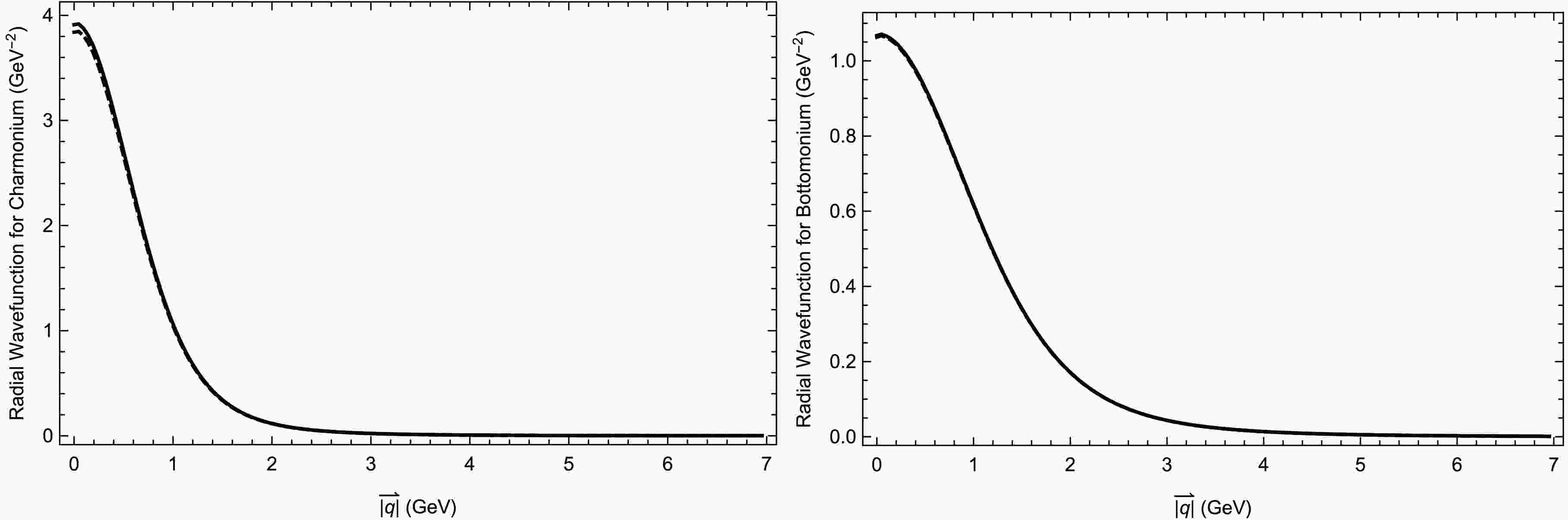
In practical calculations, we discretize Eq. (12) and solve it numerically as an eigenvalue problem to obtain reliable wave functions and mass spectra. The parameters appearing in the QCD-inspired kernel adopted in this numerical solution are listed in Table 1 and taken from Ref. [28]. They are applied identically to both pseudoscalar and vector mesons. By contrast, the parameter $ V_0 $ takes different values. These values, listed in Table 2, are fixed by matching the lowest eigenvalues to the physical masses of the lightest pseudoscalar and vector mesons. The radial wave functions for pseudoscalar and vector quarkonium states are shown in Fig. 1. The pseudoscalar and vector quarkonium curves differ slightly owing to the distinct values of $ V_0 $.

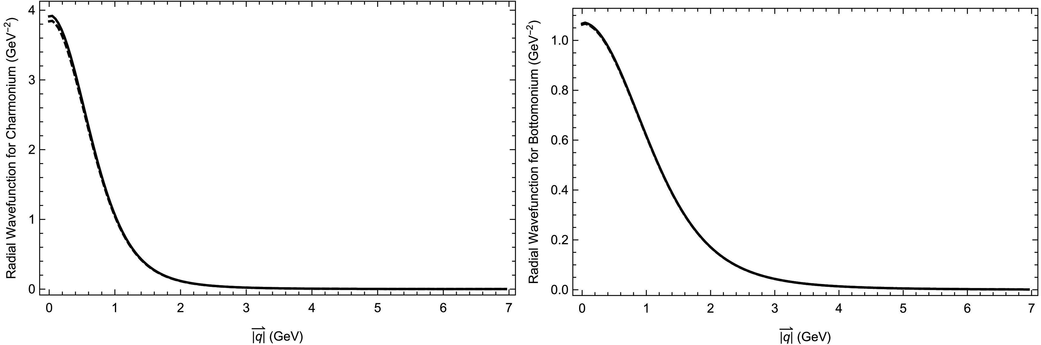
Figure 1.  Radial wave functions of the lightest $ J^{PC}=0^{-+} $ (solid) and $ J^{PC}=1^{--} $ (dashed) states. The left and right panels show the charmonium and bottomonium results, respectively.

In this section, we investigate the $ Z\to VV $ process within the BS formalism. Let $ P_{1},q_{1},\epsilon_{1} $ and $ P_{2},q_{2},\epsilon_{2} $ denote the momenta of the two quarkonia, the relativistic momenta of their constituent quarks, and the polarization vectors of the two outgoing vector quarkonia, respectively. Moreover, $ \epsilon_{z} $ denotes the polarization vector of the Z boson. We begin by evaluating the QCD amplitude, which involves two types of lowest-order Feynman diagrams, shown in Fig. 2, and the corresponding 4D-BS amplitude reads as follows: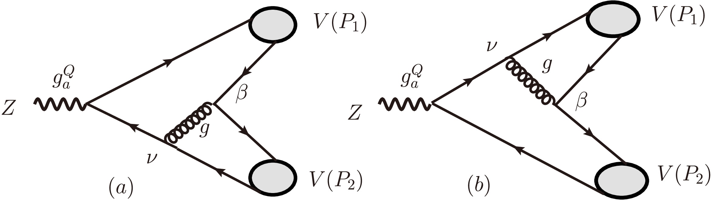

Figure 2.  Lowest-order QCD Feynman diagrams for the $ Z \to VV $ process. Two additional diagrams are obtained by permuting these two diagrams.

where $ \Psi(P_{1},q_{1}) $ and $ \Psi(P_{2},q_{2}) $ are the relativistic 4D-BS wavefunctions of the vector quarkonia, and their corresponding conjugates are defined as $ \overline{\Psi}\equiv\gamma^{0}\Psi^{\dagger}\gamma^{0} $. $ C_F = 4/3 $ is the fundamental color factor of $S U(3)$. The momenta of the quark and antiquark in both vector quarkonia are $ \dfrac{1}{2}P_{1}\pm q_{1} $ and $ \dfrac{1}{2}P_{2}\pm q_{2} $, respectively.

It can be seen that the amplitude involves integration over the relative momentum of the quark and antiquark. However, the propagators of the gluon and quark may explicitly depend on $ q_{1} $ and $ q_{2} $, which complicates the calculations. Therefore, by employing the heavy quark approximation for the propagators [22, 26, 27], we neglect the relative momentum in Eq. (14). The vertex factor for the $ ZQ\bar{Q} $ interaction is $-{\rm i}\dfrac{g}{2\cos\theta_{W}}\gamma^{\mu}\big(g_{v}^{Q}-g_{a}^{Q}\gamma^{5}\big)$. The weak SU(2)$ _{L} $ coupling constant is denoted by g, while $ \theta_{W} $ represents the Weinberg angle. The axial-vector coupling of the Z boson to a quark is given by:

where $ T_{3}^{Q} $ denotes the third component of the quark weak isospin. The strong interaction is characterized by the coupling constant $ g_{s} $ ($ \alpha_{s}=\dfrac{g_{s}^{2}}{4\pi} $), which defines the strong fine-structure constant. It can be seen that only $ g_{a}^{Q} $ survives in the amplitude $ {\cal{M}}_{{\rm{QCD}}}^{VV} $ because of charge-conjugation invariance. Using the notation of the Salpeter wave function (Eq. (3)), Eq. (14) yields a 3D amplitude:

Here, $ \overline{\psi}(q_{\perp}) $ denotes the conjugate of the 3D-BS wavefunction of vector quarkonium, as defined in Eq. (10). After taking the Dirac trace of the preceding equation, one obtains:

Finally, by squaring the amplitude, summing and averaging over the polarizations of the final and initial particles, and using the standard two-body decay formula, one obtains the decay width:

In the above expression, the factor arising from the exchange symmetry of identical particles has been considered. We introduce the quantity $\xi_{V}=\displaystyle \int\dfrac{{\rm d}^{3}\vec{q}}{(2\pi)^{3}}\phi(q_{\perp})$.

Another possible QED process is $ Z\to V+\gamma^* $, followed by the fragmentation of the off-shell photon $ \gamma^* $ into V (effectively a $ Z\to V+V $ transition via an off-shell photon), which is a rare and theoretically interesting transition in the SM. The Feynman diagram is shown in Fig. 3, and the corresponding QED-BS amplitude can be written as: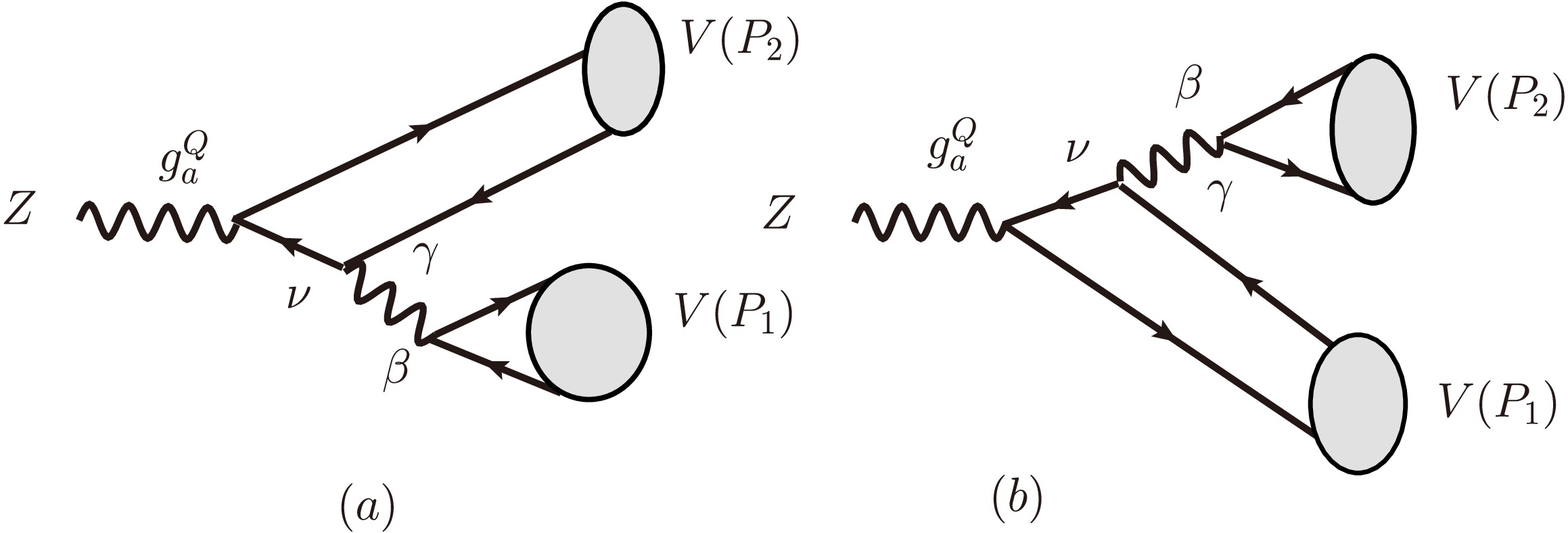

Figure 3.  Lowest-order QED Feynman diagrams for the $ Z \to VV $ process. Two additional diagrams are obtained by permuting these two diagrams.

In the above expressions, $ e_Q $ denotes the electric charge of the relevant quark. Analogously to the QCD contribution, $ g_v^Q $ also vanishes in this case.

Although the coupling vertices suppress $ {\cal{M}}_{{\rm{QED}}}^{VV} $ relative to the QCD amplitude by a factor of $ \alpha/\alpha_s $, the factor $ 1/M_V^2 $ arising from the photon fragmentation propagator substantially enhances the QED amplitude. This term is considerably larger than the $ 4/M_Z^2 $ factor from the gluon propagator in the QCD amplitude. Consequently, the QED channel dominates over the QCD channel for charmonium final states.

After evaluating the Dirac trace, we obtain:

Compared with Eq. (16), one finds that $ {\cal{M}}_{{\rm{QED}}}^{VV} $ and $ {\cal{M}}_{{\rm{QCD}}}^{VV} $ have the same structure but opposite signs. The ratio of the two amplitudes is directly given by

We adopt $ \alpha_{s}(M_{{\rm{Z}}})=0.118 $, $ \alpha_{{\rm{em}}}(M_{J/\psi})=1/132.64 $, and $ \alpha_{{\rm{em}}}(M_{\Upsilon(1S)})=1/131.87 $, consistent with the values used in Ref. [13]. The Z-boson mass, quarkonium masses, and Weinberg angle are taken from the Particle Data Group (PDG). The corresponding numerical results are $ X_{J/\psi}=-27.7 $ for charmonium and $ X_{\Upsilon(1S)}=-0.746 $ for bottomonium. Substituting the squared amplitude into the phase-space formula, we obtain the QED decay width as

The branching fractions can be calculated by using $ \Gamma/\Gamma_{t} $. Here, $ \Gamma_{t}=2.4995\ {{\rm{GeV}}} $ is the total decay width of the Z boson. In our calculations, we account for uncertainties arising from the potential parameters β, λ, and the quark masses m. We vary each parameter independently by ±10% of its central value given in Table 1, adopting the fixed-percentage variation strategy used in Refs. [23, 29]. Furthermore, whenever these parameters are adjusted, $ V_0 $ is refitted to consistently reproduce the physical meson masses. In the final calculation of the decay widths and branching fraction, all theoretical uncertainties arise solely from $ \xi_V $. The corresponding central values and uncertainty magnitudes are given below:

The predicted branching fractions calculated within both the BS and NRQCD formalisms are summarized in Table 3.

Consistent with the above analysis, incorporating QED contributions enhances the charmonium branching fraction by approximately three orders of magnitude, which is attributable to the sizable QED amplitude. By contrast, the correction for bottomonium is mild, owing to the heavier mass and smaller electric charge of the bottom quark.

Moreover, the QED and QCD amplitudes have opposite signs, leading to destructive interference that suppresses the branching ratio in the bottomonium channel. Another important point is that, for charmonium, the results are comparatively larger in the BS formalism, whereas for bottomonium, NRQCD yields comparatively larger values.

Similarly, the rare decays $ Z\to PV $ can be investigated, and the BS wave function for the pseudoscalar meson is defined in Eq. (10). This process resembles the well-known double-charmonium production process in electron-positron annihilation, $ e^{-}+e^{+}\to\eta_{c}+J/\psi $. The lowest-order QCD diagram for this transition is identical to that shown in Fig. 2, except that one vector meson is replaced by a pseudoscalar meson and $ g_a $ is replaced by $ g_v $. This process also receives contributions from both QED and QCD amplitudes. The color-singlet 3D-BS QCD amplitude can be written as:

In the above expression, $ \phi_{1}(q_{\perp1}) $ and $ \phi_{2}(q_{\perp2}) $ are the radial wave functions of the vector and pseudoscalar charmonia, respectively. In this transition, only $ g_{v}^{Q}= T_{3}^{Q}-2e_{Q}\sin^{2}\theta_{W} $ contributes, which is responsible for the vector coupling of the Z boson to the quark-antiquark pair. For simplicity, we approximate $ M_{p}=M_{v} $. Following the standard derivation, the corresponding decay width is:

Here, $ \xi_{P} $ is defined analogously to $ \xi_{V} $ for quarkonium states.

As in the $ Z\to VV $ case, we can evaluate the QED contribution to this process. The Feynman diagrams have the same structure as Fig. 3, with replacements analogous to those used in the previous QCD case. However, only two diagrams contribute, because angular momentum conservation forbids a photon from decaying into a pseudoscalar meson. The 3D-BS amplitude can be written as:

Similar to the $ Z\to VV $ case, the QED process receives an enhancement factor arising from the fragmentation mechanism. For the $ VP $ process, however, only two QED diagrams contribute. Consequently, the ratio of $ {\cal{M}}_{{\rm{QED}}}^{VP} $ to $ {\cal{M}}_{{\rm{QCD}}}^{VP} $ is equal to one-half of $ X_{V} $ given in Eq. (20). The corresponding decay width is:

We adopt the same set of uncertainty sources as for the $ Z\to VV $ process:

Finally, the branching-fraction values predicted by our model and by recent NRQCD studies are presented in Table 4.

Similar to the $ Z\to VV $ process, the QED contributions are significant in this case. Moreover, we again observe destructive interference due to the opposite signs of the QED and QCD amplitudes. Furthermore, whereas NRQCD predictions are larger for bottomonium production, our results are comparatively larger for charmonium.

We have introduced another possible LO channel for the Z boson decay into double S-wave quarkonia, in which the Z boson decays into bottomonium plus charmonium via a QED amplitude. The decay processes are $ Z\to J/\psi+\Upsilon(1S) $, $ Z\to\eta_{b}+J/\psi $, and $ Z\to\eta_{c}+\Upsilon(1S) $. We investigate these processes one by one.

We begin with $ Z\to J/\psi+\Upsilon(1S) $. The Feynman diagram is similar to Fig. 3; one only needs to replace the charmonium vector with a bottomonium vector. The corresponding 3D-BS amplitude is:

In the above expression, $ \varepsilon_{1} $ and $ \varepsilon_{2} $ denote the polarization vectors, while $ \phi_{J/\psi}(q_{\perp1}) $ and $ \phi_{\Upsilon(1S)}(q_{\perp2}) $ denote the radial wave functions of vector charmonium and vector bottomonium, respectively. The two terms inside the brackets in Eq. (28) correspond to two distinct virtual-photon exchange channels: $ Z\to \Upsilon(1S)+\gamma^{\ast} $ with $ \gamma^{\ast}\to J/\psi $, and $ Z\to J/\psi+\gamma^{\ast} $ with $ \gamma^{\ast}\to \Upsilon(1S) $, respectively. For brevity, we approximate $ \alpha_{{\rm{em}}}(M_{\Upsilon(1S)})=\alpha_{{\rm{em}}}(M_{J/\psi}) $. This transition proceeds via $ g_{a}^{Q} $, and the factors $ d_{1} $ and $ d_{2} $ are defined below:

Since the two outgoing particles have different masses, the magnitude of the three-momentum of each particle is given by:

Finally, we obtain the corresponding decay width:

For brevity, we have introduced $ A_{VV} $ in Eq. (29); the full expression is provided in the Appendix. Equation (21) can be readily recovered from Eq. (29) by substituting $ M_{J/\psi}=M_{\Upsilon(1S)}=M_{V} $, $ \xi_{J/\psi}=\xi_{\Upsilon(1S)}=\xi_{V} $, $ e_{c}=e_{b}=e_{Q} $, and $ g_{a}^{b}=g_{a}^{c}=g_{a}^{Q} $, together with an additional factor of $\dfrac{1}{2}$ (due to quantum statistics for identical particles). The corresponding numerical value of the branching fraction for the $ J/\psi+\Upsilon(1S) $ process is given in Table 5.

We now analyze $ Z\to\eta_{b}+J/\psi $ and $ Z\to\eta_{c}+\Upsilon(1S) $. As in $ Z\to PV $, these processes also have only two LO Feynman diagrams. The decay $ Z\to\eta_{b}+J/\psi $ proceeds via $ g_{v}^{b} $, while $ Z\to\eta_{c}+\Upsilon(1S) $ proceeds via $ g_{v}^{c} $. Here, $ g_{v}^{c} $ and $ g_{v}^{b} $ denote the vector couplings at the Z-boson vertices to $ (c\bar{c}) $ and $ (b\bar{b}) $, respectively. The corresponding 3D-BS amplitudes for both processes read as:

In Eq. (30) and Eq. (31), $ \varepsilon_{1} $ and $ \varepsilon_{2} $ denote the polarization vectors of charmonium and bottomonium, respectively. The factors $ l_{1} $ and $ l_{2} $ are given by:

Expressions for the decay widths of these processes can be obtained using the previous procedure:

For simplicity, $ A_1 $ and $ A_2 $, introduced in Eqs. (32) and (33), respectively, are presented in full in the Appendix. Equation (26) can also be reproduced by replacing the corresponding bottomonium parameters with those of charmonium, or vice versa. The branching fractions for both processes are also listed in Table 5.

As expected, the branching fraction for $ Z\to J/\psi+\Upsilon(1S) $ lies between those for the QED amplitudes of $ Z\to J/\psi+J/\psi $ and $ Z\to\Upsilon(1S)+\Upsilon(1S) $. Similarly, the branching fraction for $ Z\to\eta_{b}+J/\psi $ lies between those for $ Z\to J/\psi+\eta_{c} $ and $ Z\to\Upsilon(1S)+\eta_{b} $. However, the branching fraction for the process $ Z\to\eta_{c}+\Upsilon(1S) $ does not follow this pattern and is comparatively smaller. The reason is that the Z boson decays through the vector coupling $ g_{v}^{c} $, which is weaker than $ g_{v}^{b} $, and a virtual photon can more easily decay into lighter particles ($ M_{J/\psi} $) than into heavier ones ($ M_{\Upsilon(1S)} $).

Our results agree in order of magnitude with the LO NRQCD predictions. Remarkably, both the NLO radiative and relativistic corrections make large negative contributions to this process, reducing the LO predictions to roughly 30% of their original magnitude.

The rare radiative decay of the Z boson into a quarkonium state plus a photon, $ Z\to X(Q\bar{Q})\gamma $, provides a valuable probe of non-perturbative aspects of QCD. In the SM, such decays proceed primarily through secondary production mechanisms, in which the Z boson decays into a pair of heavy quarks that subsequently bind radiatively into the final quarkonium state. The general 3D-BS amplitude corresponding to Fig. 4 can be written as,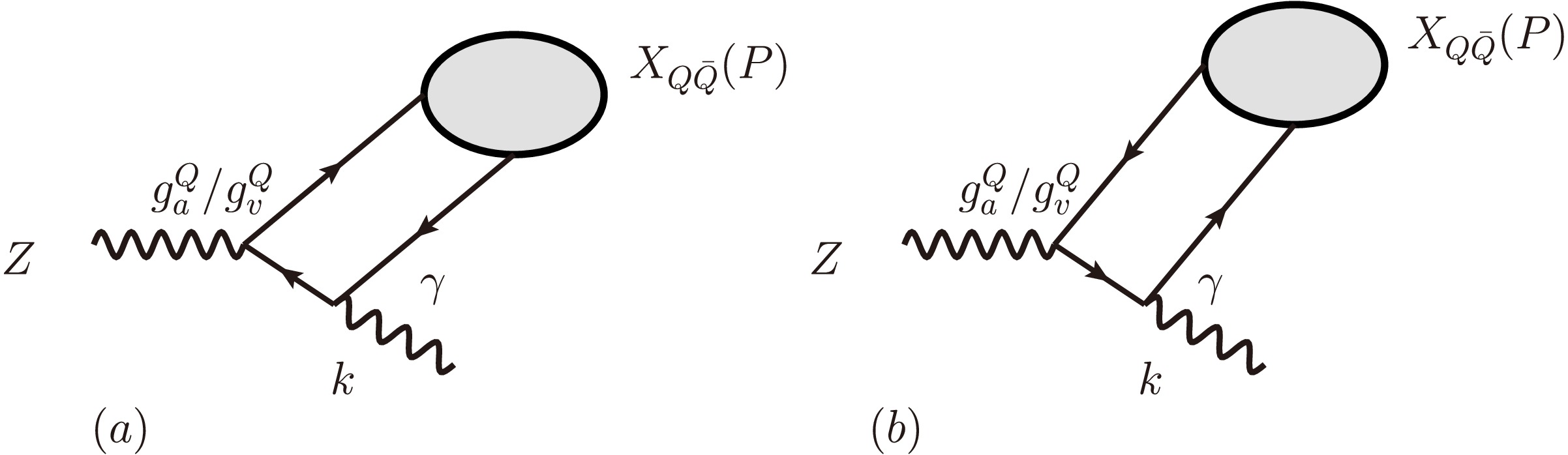

Figure 4.  Lowest-order Feynman diagrams for the $ Z\to X(Q\bar{Q})\gamma $ process.

Here, $ \psi(q_{\perp}) $ is the 3D-BS wave function of vector or pseudoscalar quarkonium, and k and $ \epsilon_{\gamma} $ denote the momentum and polarization vector of the radiative photon, respectively. After substituting the BS wave function of the corresponding quarkonium into Eq. (34) and taking the Dirac trace, we obtain the amplitudes:

Due to charge-conjugation invariance, $ {\cal{M}}_{Z\to P\gamma} $ proceeds via $ g_{v}^{Q} $, whereas $ {\cal{M}}_{Z\to V\gamma} $ proceeds via $ g_{a}^{Q} $. The two-body radiative decay width for $ Z\to X(Q\bar{Q})+\gamma $ can be defined as follows:

Here, $ M_{X(Q\bar{Q})} $ and $ {\cal{M}} $ denote the mass and amplitude of the corresponding quarkonium, respectively. To derive the analytical decay widths of the pseudoscalar and vector quarkonia, we substituted Eq. (35) into Eq. (36) and carried out straightforward mathematical manipulations:

Finally, the branching fractions are calculated following the usual procedure and are presented in Table 6.

One can observe in Table 6 that the values for the vector quarkonium are comparatively larger than those for the pseudoscalar quarkonium. The primary reason is that the production of $ \eta_{c}(\eta_{b})+\gamma $ proceeds through the vector coupling, whereas the production of $ J/\psi(\Upsilon)+\gamma $ proceeds through the axial-vector coupling of the Z boson, and the axial-vector coupling is stronger than the vector coupling in these transitions. Moreover, similar to double quarkonium production, the BS results are larger for charmonium, whereas the NRQCD results are larger for bottomonium.

For the first time, we employ the BS formalism to investigate the rare decays of the Z boson into S-wave quarkonia. These decay modes include double S-wave charmonia, double S-wave bottomonia, associated S-wave charmonium–bottomonium pairs, and radiative decays of the Z boson into S-wave quarkonia. At present, these decays are being actively investigated both experimentally and theoretically. Our primary focus is on non-perturbative effects; therefore, we use the BS model, which is well suited to describing such effects, since relativistic effects play an important role in hadronization, particularly for charmonium. For the double-quarkonium decay modes, we consider the amplitudes of both the QCD and QED channels and find that the QED amplitude makes a significant contribution. However, destructive interference occurs because of the opposite signs of these two amplitudes. The total branching ratios are therefore far below the current experimental limits recently reported by the CMS Collaboration [4]. For the Z boson decay modes into bottomonium plus charmonium through the QED amplitude alone, the calculated branching fraction of $ Z\to J/\psi+\Upsilon(1S) $ lies, as expected, between those for the QED-only processes $ Z\to J/\psi+J/\psi $ and $ Z\to\Upsilon(1S)+ \Upsilon(1S) $. Following the same trend, the branching fraction of $ Z\to\eta_{b}+J/\psi $ lies between those of $ Z\to J/\psi+\eta_{c} $ and $ Z\to\Upsilon(1S)+\eta_{b} $. In contrast, the branching fraction for $ Z\to\eta_{c}+\Upsilon(1S) $ is considerably smaller. For radiative Z boson decays, our results for the charmonium channels are consistent with the latest upper limits set by the ATLAS Collaboration [5].

Additionally, it is noteworthy that charmonium production yields larger values within the BS formalism, whereas bottomonium production yields larger values within NRQCD. This indicates that charmonium is intrinsically relativistic, whereas bottomonium is non-relativistic. This picture is consistent with the fact that the BS model is a covariant approach that naturally incorporates relativistic corrections, whereas NRQCD is formulated within a non-relativistic framework. Further evidence supporting this conclusion comes from calculations of the cross section for the process $ e^+e^-\to J/\psi+\eta_{c} $ at B factories. In Refs. [26, 27, 33], the authors computed the cross section for the LO amplitude using the BS model and obtained values of $ 22.3 $ fb, $ 20.7 $ fb, and $ 21.75 $ fb, respectively. These values lie between the experimental results from Belle ($ 25.6 $ fb) [34, 35] and BaBar ($ 17.6 $ fb) [36]. In contrast, the LO contribution within NRQCD is far too small [37, 38]. To resolve this discrepancy, substantial higher-order corrections, either in $ \alpha_{s} $ [39, 40] or from relativistic effects [41−43], are required; these amount to nearly twice the LO value [38]. Recently, theoretical calculations for this process have been extended to order $ \alpha_s^2 $, providing a more precise theoretical basis [44, 45].

An important point to note is that the only difference between the BS predictions in the heavy-quark limit, as calculated in Ref. [26] and in our work, and the LO NRQCD results for both $ e^{+}e^{-}\rightarrow J/\psi+\eta_{c} $ and rare Z boson decays into S-wave quarkonia lies in the non-perturbative part (the radial wave function). For charmonium systems, the quark–antiquark relative velocity squared typically takes the value $ v^{2}\approx0.3 $, leading to sizable relativistic corrections. Although our numerical implementation employs the instantaneous approximation and heavy-quark-limit simplifications, the BS formalism may still capture essential relativistic kinematic effects that are not fully included at LO in the NRQCD expansion. For bottomonium, $ v^{2}\approx0.1 $, and the non-relativistic NRQCD expansion becomes the preferred approach within its expected regime of validity.

Rare Z boson decays could nevertheless provide a promising probe of new physics, and we hope that further searches for these decays will be carried out at upcoming high-luminosity facilities, such as the FCC-ee, ILC, CEPC, and Super Z factory.

The authors would like to express their gratitude to Dr. Xiao-Peng Wang, who performed the LO NRQCD calculations for associated charmonium–bottomonium decay processes.

Below, we present the complete expressions for $ A_{VV} $, $ A_{1} $, and $ A_{2} $, as defined in Eqs. (29), (32), and (33), respectively, for the corresponding charmonium–bottomonium decay processes