Quasinormal frequencies and greybody factors for axial perturbations of dilaton–Euler–Heisenberg de Sitter black holes

Originally established in 1936 [1], the Euler-Heisenberg (EH) effective action provides a crucial nonlinear generalization of standard quantum electrodynamics (QED). This framework effectively captures vacuum polarization phenomena within a classical formalism, particularly in scenarios involving intense electromagnetic fields. Rather than treating the vacuum as empty space, EH theory describes it as a medium capable of polarization and magnetization [2]. In addition to refining classical electrodynamics in strong-field regimes, this theory has become fundamental to the study of nonlinear phenomena in astrophysics and cosmology.

Leveraging these distinctive properties, the first Einstein-Euler-Heisenberg (EEH) black hole solution—an anisotropic, magnetically charged configuration resembling the Reissner-Nordström metric but incorporating dyonic degrees of freedom—was obtained in 1956 [3]. Subsequent work extended this framework to electrically charged solutions [3, 4], rotating black holes [5–7], and models within modified gravity theories [8, 9]. More recently, inspired by string theory and Lovelock gravity, Ref. [10] proposed an extension of Einstein-Maxwell-dilaton theory by coupling the dilaton field to EH electrodynamics in a novel manner. Further investigations have explored particle dynamics, gravitational lensing [11, 12], and shadow properties [13] around dilaton–Euler–Heisenberg (dEH) black holes. Jiang et al. [14] also analyzed the structure of geometrically thin, optically thick accretion disks in these spacetimes.

The recent detection of gravitational waves has opened new avenues for studying strong gravitational fields near black holes. During the ringdown phase of a binary compact star merger, the emitted gravitational waves can be modeled as the response of the remnant black hole to spacetime perturbations. At this stage, the remnant is well described by a perturbed black hole solution. These waves exhibit characteristic decay timescales and are naturally described by quasinormal modes (QNMs) [15, 16]. Moreover, QNMs provide unique probes for testing the no-hair conjecture through their frequency spectra [17–19]. In the context of modified gravity theories [20–23], QNMs serve as essential tools, as their behavior under parametric perturbations and background spacetime deformations places strong constraints on alternative gravitational frameworks. Furthermore, investigating QNM stability helps assess whether a background spacetime is stable against small perturbations of the effective potential [24–29].

Another crucial aspect of black hole perturbation theory is the greybody factor [30–34], which characterizes how a black hole's effective potential filters the spectrum of emitted radiation. In gravitational-wave astronomy, greybody factors and QNMs form a complementary framework: QNMs determine the ringdown phase through their characteristic frequencies and damping times, whereas greybody factors quantify the frequency-dependent transmission probability of gravitational waves propagating through the background spacetime [35, 36].

These issues are particularly relevant for dEH black holes in string-inspired Euler-Heisenberg gravity. To date, the QNMs and greybody factors of dEH black holes for test scalar and electromagnetic fields have been computed in asymptotically flat [37] and de Sitter [38] spacetimes. In addition, we have analyzed the polar metric perturbations [39] and the axial gravitational modes in the asymptotically flat case [40]. Extending this line of research, the present paper focuses on axial gravitational and electromagnetic perturbations in the de Sitter background.

This paper is organized as follows. In Section II, we briefly review the black hole solution and derive the master equations for axial perturbations. In Section III, we outline the AIM and WKB methods and then present the numerical results for the quasinormal frequencies, analyzing their parameter dependence in detail. In Section IV, we calculate the greybody factors using the WKB approach and discuss their physical implications. Finally, conclusions and discussion are presented in Section V. Throughout this paper, we adopt geometrized units in which $ G = c = 1 $ and the metric signature is $ (-, +, +, +) $.

Recently, Bakopoulos et al. [10] introduced a novel Einstein-Maxwell-dilaton theory that incorporates a nonlinear Euler-Heisenberg term with explicit dilaton coupling

where R denotes the scalar curvature, ϕ is the scalar field, $ \mathfrak{V(\phi)} $ is the scalar potential, and $ {\cal L} $ represents the Lagrangian density describing the coupling between the scalar field and the nonlinear electromagnetic field, with $ \mathfrak{V(\phi)} $ and $ {\cal L} $ taking the form

where Λ is a positive cosmological constant, $ f(\phi) $ is a coupling function, $ F^2=F_{\mu\nu}F^{\mu\nu} $, and $ F^4=F_{\mu\nu}F^{\mu\nu}F_{\rho\delta}F^{\rho\delta} $. Here, $ F_{\mu\nu} $ denotes the usual field strength, $ F_{\mu\nu}= \partial_\mu A_{\nu}-\partial_{\nu}A_{\mu} $, and the function $ f(\phi) $ is given by $f(\phi) = -\dfrac{1}{2}\left(3{\rm e}^{-2\phi}+3{\rm e}^{2\phi}+4\right)$. If one sets $ \alpha=\beta=0 $, the model reduces to the standard Einstein-Maxwell-dilaton theory. Varying the action (1) with respect to the metric yields the Einstein equation

where $ G_{\mu\nu} $ is the Einstein tensor, and the energy-momentum tensor takes the form

the scalar equation is given by

the Maxwell equation leads to

For convenience, we define $ \epsilon \equiv \alpha-\beta $. The magnetically charged black hole solution in de Sitter spacetime can be written as [10, 38]

Note that the magnetic gauge potential is $ \boldsymbol{A}_\mu= (0,0,0,Q_{\rm m}\cos\theta) $, where M and $ Q_{\rm m} $ denote the black hole mass and magnetic charge, respectively.

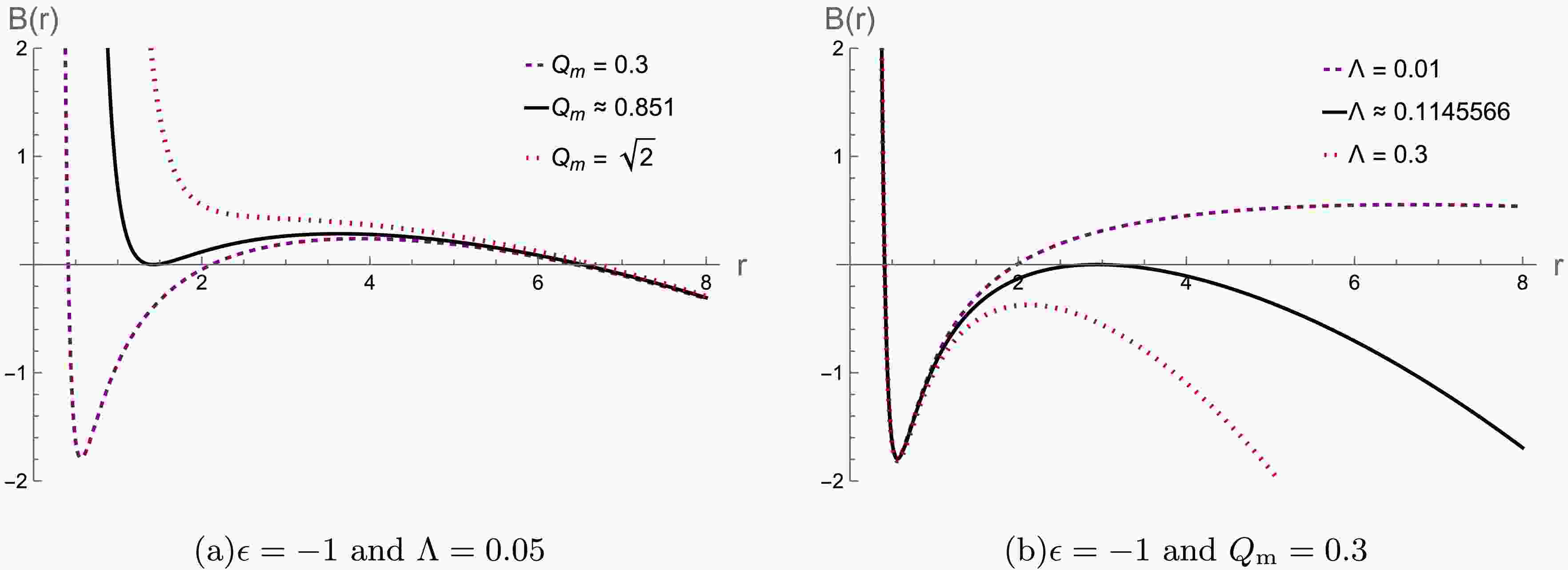
The parameter $ \epsilon $ strongly influences the horizon structure of the spacetime, producing qualitatively distinct geometrical configurations across different regions of parameter space, as illustrated in Figs. 1 and 2.

Figure 1.  (color online) The metric function $ B(r) $ as a function of the radial coordinate r, with $ M=1 $.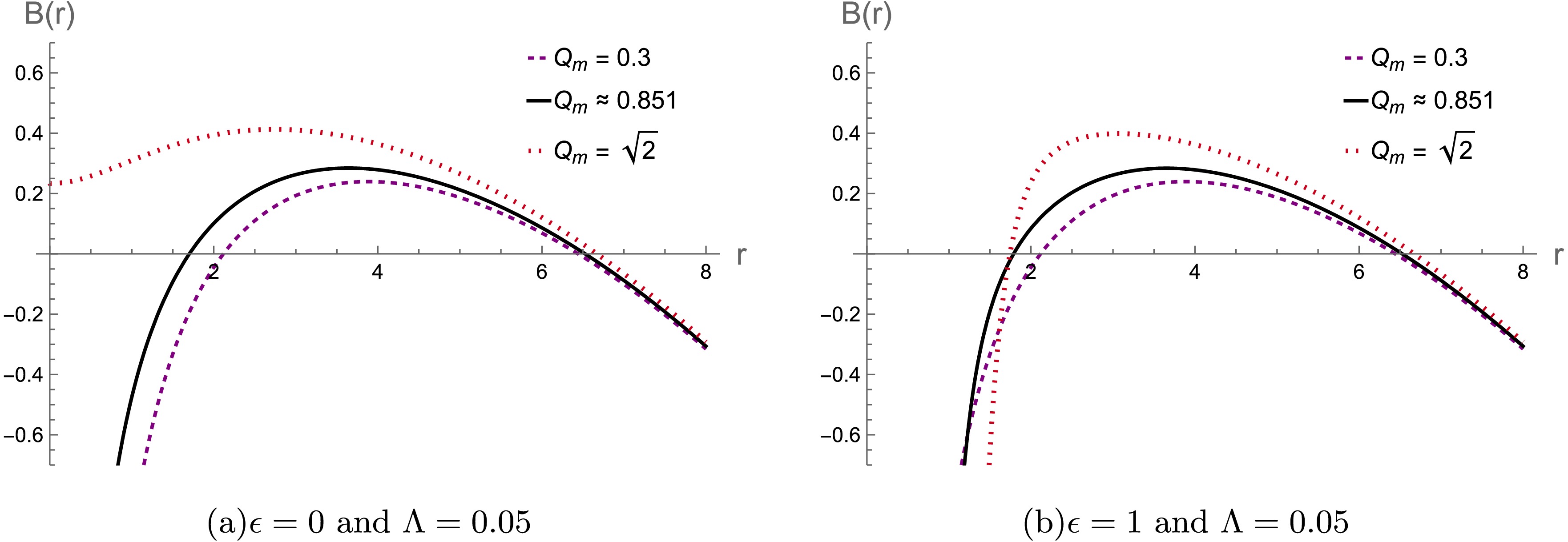

Figure 2.  (color online) The metric function $ B(r) $ as a function of the radial coordinate r, with $ M=1 $.

For $ \epsilon \lt 0 $, the spacetime exhibits a rich horizon structure and can accommodate up to three distinct horizons: a Cauchy (inner) horizon, a black hole event horizon, and a cosmological horizon. The left panel of Fig. 1 demonstrates the effect of the magnetic charge $ Q_{\text{m}} $ for a fixed cosmological constant Λ. As $ Q_{\text{m}} $ increases, the Cauchy horizon and the event horizon gradually approach each other and eventually merge at a critical value ($ Q_{\text{m}} \approx 0.851 $), forming an extremal black hole. When the charge increases further (e.g., $ Q_{\text{m}} = \sqrt{2} $), the black hole horizons disappear entirely. In this regime, the central singularity is no longer hidden by an event horizon, resulting in a naked singularity surrounded only by the cosmological horizon. The right panel of Fig. 1 illustrates the influence of the cosmological constant Λ for a fixed magnetic charge. As Λ increases, the black hole event horizon expands outward, while the cosmological horizon shrinks inward, until the two coincide ($ \Lambda \approx 0.1145 $), corresponding to the Nariai limit. For even larger values of Λ, the black hole and cosmological horizons disappear, driving the spacetime into another naked-singularity phase.

In contrast, the horizon structures for $ \epsilon = 0 $ and $ \epsilon \gt 0 $ are considerably less complex, as shown in Fig. 2. In these regimes, the spacetime typically possesses a standard two-horizon structure, consisting of an event horizon and a cosmological horizon, within the considered parameter ranges. For $ \epsilon = 0 $ (the left panel of Fig. 2), the peak of the metric function $ B(r) $ decreases as $ Q_{\text{m}} $ increases, indicating a trend toward an extremal configuration near $ Q_{\text{m}} = \sqrt{2} $. However, for $ \epsilon = 1 $ (the right panel of Fig. 2), the nonlinear electrodynamic effects significantly suppress the influence of the magnetic charge. Consequently, the qualitative horizon structure remains stable and essentially unchanged throughout the examined parameter space.

The study of black hole perturbations was initiated by Regge and Wheeler [41], who focused on odd-parity spherical harmonic modes, and was subsequently extended to even-parity modes by Zerilli [42]. This work focuses specifically on odd-parity perturbations to simplify the theoretical framework. We treat the perturbed metric as the sum of the unperturbed background metric $ \bar{g}_{\mu\nu} $ and the perturbation itself, $ \delta{g}_{\mu\nu} $:

Working within the Regge–Wheeler gauge formalism [43], we decompose the metric perturbations into tensor spherical harmonics. In the odd-parity (axial) sector, the gravitational perturbation is characterized by two radial functions, $ h_0(r) $ and $ h_1(r) $, which lead to the following metric ansatz:

where the spherical harmonics can, without loss of generality, be replaced by Legendre polynomials by setting the azimuthal number to $ m=0 $, i.e., $ Y_{lm}|_{m=0}= \sqrt{\dfrac{2l+1}{4\pi}}P_{l}(\cos\theta) $, because the background metric is spherically symmetric. Similarly, we express the vector perturbations as

where $ \bar{A}_{\mu} $ denotes the background electromagnetic field, and $ \delta{A}_{\mu} $ represents the corresponding perturbations. We analyze the axial gauge transformation, with the gauge vector taking the following specific form:

Substituting the perturbed metric and vector potential (Eqs. (11), (12), (13), and (14)) into the field equation (4), we obtain the nonzero components of the first-order perturbed gravitational field equations as follows:

with the Lagrangian density $\overline {\cal{L}} $. Its explicit form for the black hole solutions (10) can be written as

From Eqs. (15), (16), and (17), we obtain the perturbation function $ u_3(r)=0 $. Moreover, this function does not appear in the gravitational perturbation equations, Eqs. (18), (19), and (20), which clearly demonstrates that the axial gravitational perturbations are decoupled from the electromagnetic ones. This decoupling of the metric and gauge-field sectors is consistent with previous studies of magnetic black holes [44−46], allowing us to treat the gravitational sector independently.

We now focus on axial electromagnetic perturbations. We restrict our analysis to the axial sector because polar perturbations generally involve more complicated couplings among the metric, electromagnetic, and dilaton fields; see Ref. [39] for a recent study of the coupled metric–dilaton sector. Substituting the perturbed metric and vector potential, given in Eqs. (11), (12), (13), and (14), into the Maxwell equation (8), we obtain the corresponding perturbed equations

From these equations, it can be seen that the gravitational perturbation functions $ h_0(r) $ and $ h_1(r) $ must vanish, and that there exists only a single perturbation equation for the perturbed electromagnetic field.

It is well known that gravitational perturbations are central to black hole physics because they directly probe spacetime geometry, align with observational priorities in gravitational-wave astronomy, and reflect the black hole's intrinsic properties. In the following section, we focus only on axial gravitational perturbations. From Eqs.(18), (19), and (20), it is readily verified that only two of the above three equations are independent. Considering the component $ E_{\theta\varphi}^{(g)} $ in (20), we have

Substituting Eq. (26) into the component $ E_{r\varphi}^{(g)} $ (19) eliminates $ h_0(r) $ and $ h_0'(r) $, yielding a single second-order differential equation for $ h_1(r) $. To cast this master equation into the standard Schrödinger form, we further define the function $ \Psi_G(r) $ as

We assume that the function $ C_0(r) $ takes the following form

and then obtain the final perturbed equation

where $ r_* $ denotes the tortoise coordinate

Substituting Eq. (21) into Eq. (29) and simplifying, we obtain the effective potential $ V_G(r) $ as

with the Lagrangian density $ {\cal \bar{L}} $. Its explicit form for the black hole solutions (10) can be written as

We should note that the perturbation of the electromagnetic part of the energy-momentum tensor cannot be ignored. A similar phenomenon also appears in Ref. [47].

Note that the solutions (10) and the potential (31) are invariant under the following rescaling: $ r/M\rightarrow r $, $ Q_{\text{m}} /M\rightarrow Q_{\text{m}} $, and $ \epsilon/ M^2\rightarrow \epsilon $. For a clearer analysis of the behavior of the potential function, we set $ M=1 $ throughout the paper and leave $ \epsilon $ and $ Q_{\text{m}} $ free, without loss of generality. The effective potentials $ V_G(r) $ are plotted in Figs. 3 and 4, respectively. It is evident that the height of the effective potential increases as $ Q_{\text{m}} $ increases. Moreover, the potential also increases with increasing multipole moment l in both cases. It is worth pointing out that the effective potentials are always positive, indicating that the system is stable under axial gravitational field perturbations.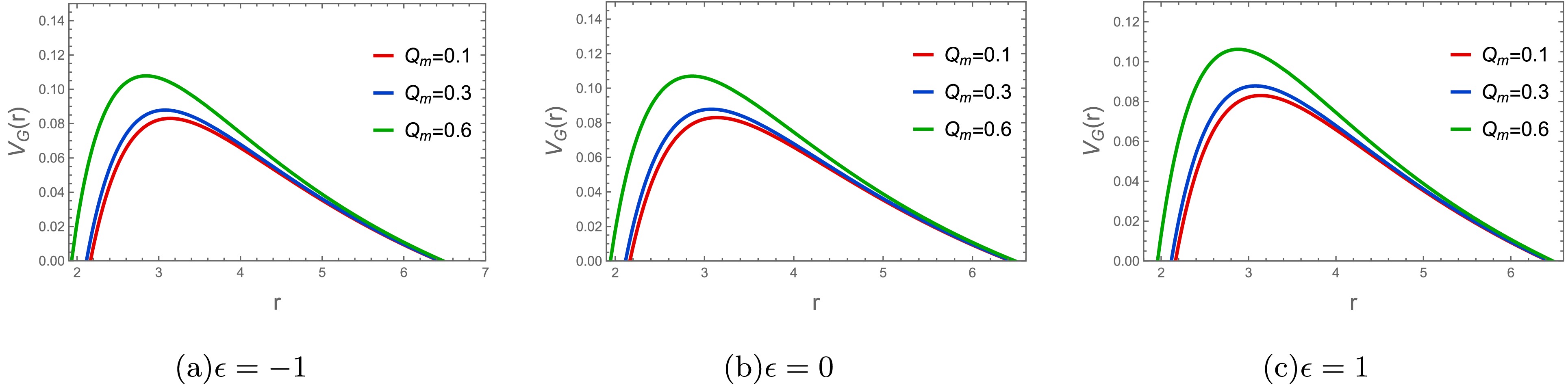

Figure 3.  (color online) The effective potential $ V_{\mathrm{G}}(r) $ for gravitational field perturbations ($ l=2 $) is shown as a function of the radial coordinate r for different values of the magnetic charge $ Q_{\mathrm{m}} $. In all cases, we set $ M=1 $ and $ \Lambda=0.05 $. Panels (a), (b), and (c) correspond to $ \epsilon=-1 $, $ \epsilon=0 $, and $ \epsilon=1 $, respectively. As $ Q_{\mathrm{m}} $ decreases, the peak of the potential barrier shifts outward, and its height is significantly suppressed.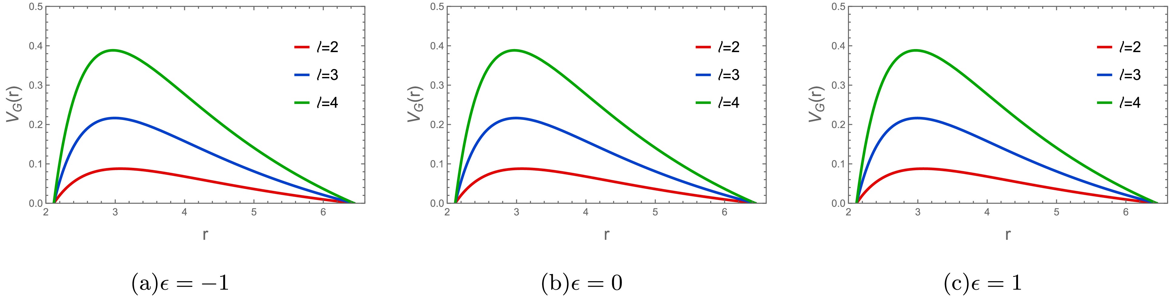

Figure 4.  (color online) The effective potential $ V_{\mathrm{G}}(r) $ for gravitational field perturbations (with $ Q_{\mathrm{m}}=0.3 $) is shown as a function of the radial coordinate r for different values of the angular quantum number l. In all cases, we set $ M=1 $ and $ \Lambda=0.05 $. Panels (a), (b), and (c) correspond to $ \epsilon=-1 $, $ \epsilon=0 $, and $ \epsilon=1 $, respectively. As l increases, the peak of the potential barrier shifts to the right, and its height increases significantly.

To cast this master equation (25) into the standard Schrödinger form, we further define the function $ u_3(r) $ as follows:

We assume that the function $ C_1(r) $ takes the following form

and then obtain the final perturbed equation

where

The radial profile of the effective potential $ V_E(r) $ exhibits distinct features for different combinations of the magnetic charge $ Q_{\mathrm{m}} $ and angular quantum number l, as shown in Figs. 5 and 6. Importantly, for all parameter sets considered, the potential remains positive throughout the exterior spacetime region ($ r_{\mathrm{h}}<r<r_{\mathrm{c}} $). This persistent positivity, particularly the absence of any negative potential well, provides strong evidence for the structural stability of the black hole against electromagnetic field perturbations. Furthermore, quantitative analysis reveals that, for $ \epsilon=1 $, the height of the potential barrier is anomalously suppressed as $ Q_{\mathrm{m}} $ increases, indicating a distinct geometric dependence induced by the nonlinear electrodynamics, in contrast to the monotonically increasing behavior observed for $ \epsilon\leqslant 0 $.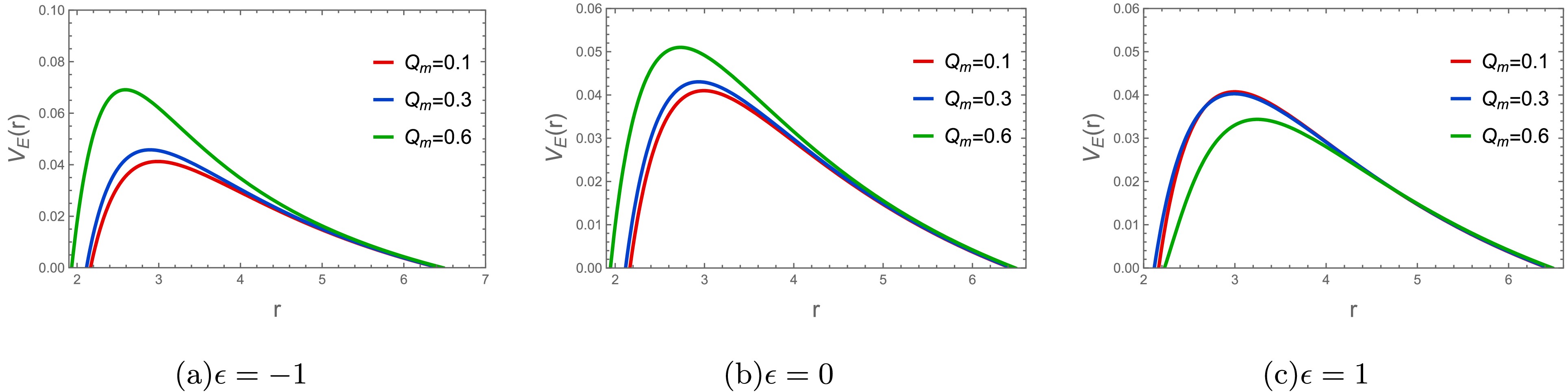

Figure 5.  (color online) The effective potential $ V_{\mathrm{E}}(r) $ for electromagnetic field perturbations ($ l=1 $) is shown as a function of the radial coordinate r for different values of the magnetic charge $ Q_{\mathrm{m}} $. In all cases, we set $ M=1 $ and $ \Lambda=0.05 $. Panels (a), (b), and (c) correspond to $ \epsilon=-1 $, $ \epsilon=0 $, and $ \epsilon=1 $, respectively.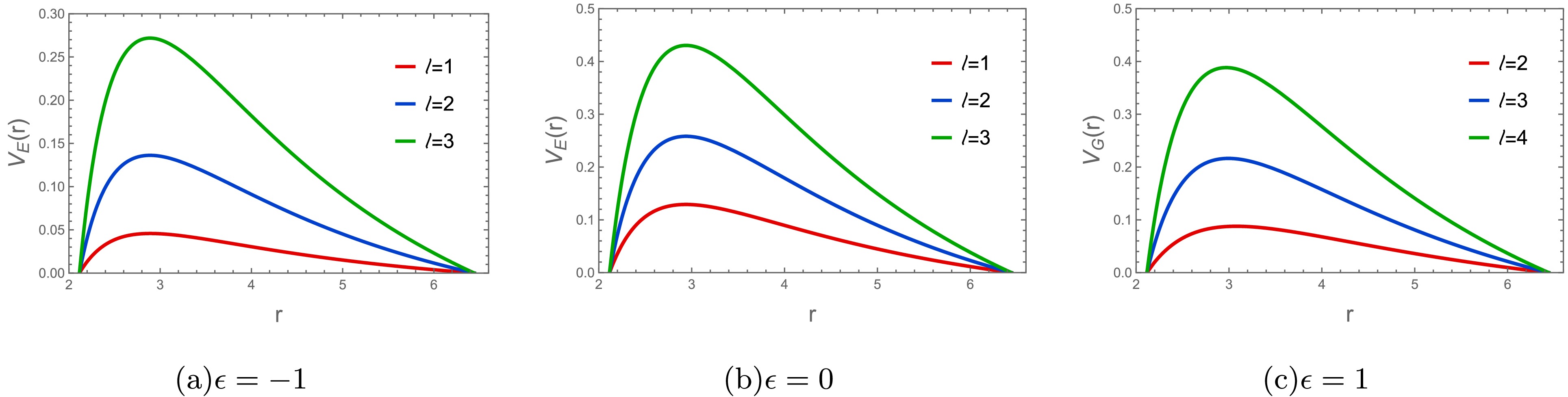

Figure 6.  (color online) The effective potential $ V_{\mathrm{E}}(r) $ for electromagnetic field perturbations with $ Q_{\mathrm{m}}=0.3 $ is shown as a function of the radial coordinate r for different values of the angular quantum number l. In all cases, we set $ M=1 $ and $ \Lambda=0.05 $. Panels (a), (b), and (c) correspond to $ \epsilon=-1 $, $ \epsilon=0 $, and $ \epsilon=1 $, respectively. As l increases, the peak of the potential barrier shifts to the right, and its height increases significantly.

To compute the quasinormal spectra rigorously, we employ a combination of the Asymptotic Iteration Method (AIM) [48–51] and the WKB approximation [52–55]. By applying these two independent numerical techniques, we ensure the reliability of our frequency data through mutual verification.

In this section, we present the main steps of the AIM method. First, we rewrite the axial metric perturbation equation (29) in terms of $ u=1/r $

To characterize the divergent behavior at the cosmological and event horizons, we define

where $ \chi(u) $ is a finite, convergent function. To establish the appropriate scaling behavior that satisfies the quasinormal mode boundary conditions, we define

where $ \kappa_j $ denotes the surface gravity evaluated at the coordinate $ u_j $, defined by the condition $ B(u_j)=0 $. This scaling transformation regularizes the solution by removing the divergent behavior near the boundary at $ u_j $ and simultaneously enforcing the boundary conditions. We define the surface gravity at the event horizon as follows:

Here, $ r_h $ and $ r_c $ denote the radii of the black-hole event horizon and the cosmological horizon, respectively. Both are positive roots of the metric function $ B(r)=0 $ and satisfy $ r_h<r_c $. If a Cauchy horizon is present, its radius $ r_- $ satisfies $ r_-<r_h<r_c $. A similar analysis of the surface gravity and horizon boundary conditions for quasinormal modes of black holes with a cosmological constant can be found in Ref. [55]. Substituting Eq. (37) into the perturbation equation in the u domain, we obtain

where

and

Based on $ \lambda_\mathrm{0} $ and $ s_\mathrm{0} $, the perturbed equation (40) can be solved numerically using the improved $ \mathrm{AIM} $ [48]. Following the same procedure described above, one can systematically derive the corresponding coefficient functions $ \lambda_0 $ and $ s_0 $ for electromagnetic field perturbations. Owing to their cumbersome and lengthy analytical forms, we do not present them explicitly here for brevity. Nevertheless, these expressions are implemented exactly in our numerical codes to compute the quasinormal frequencies in the electromagnetic sector.

To analyze the spectral properties in the frequency domain, we employ the semi-analytic WKB approximation technique [31, 52]. This approach is particularly effective for scattering problems involving potential barriers and has been widely applied in black hole physics. This method, first proposed by Schutz and Will, was used to study black hole scattering problems [56]. It was subsequently further developed by Iyer, Will, and Konoplya [31]. In this paper, we consider the widely used sixth-order WKB approximation method [31]

where $ V''(r_0) $ is the second derivative of the effective potential with respect to $ r_* $, evaluated at its maximum point $ r_0 $, which is defined by the solution of the equation $\left. \dfrac{{\rm d}V}{{\rm d}r_*} \right|_{r_*=r_0}= 0$. $ V_0 $ denotes the maximum value of the effective potential, and $ \Lambda_i $ represents the ith-order correction terms that depend on the values of the effective potential. This semi-analytical method has been applied extensively to numerous black hole spacetimes.

It should be pointed out here that the WKB approach works well when the multipole number is larger than or equal to the overtone number, i.e., $ l\geq n $; by contrast, it yields less accurate results for $ l<n $ [53, 54].

By analyzing these errors, we provide a detailed assessment of the accuracy of our QNM estimates. We further consider the percentage deviation $ \Delta_{AW} $ of QNMs obtained using the AIM and WKB methods. The relative error $ \Delta_{AW} $ between the two methods is defined by

Tables 1, 2, and 3 summarize the fundamental ($ n=0 $) quasinormal frequencies for both axial gravitational and electromagnetic perturbations. The results obtained from the AIM and WKB approaches show excellent agreement. The relative error $ \Delta_{AW} $ is typically well below $ 0.1\% $, confirming the reliability of our numerical data.

We first analyze the effect of the magnetic charge $ Q_{\text{m}} $, as shown in Table 1 and Fig. 7. Both the real part of the frequency $ \operatorname{Re}(\omega) $ and the magnitude of the imaginary part $ |\operatorname{Im}(\omega)| $ generally increase with increasing $ Q_{\text{m}} $, except for the anomalous electromagnetic branch with $ \epsilon=1 $. Here, $ \operatorname{Re}(\omega) $ denotes the oscillation frequency of the perturbation, whereas $ |\operatorname{Im}(\omega)| $ denotes the damping rate. This implies that a larger magnetic charge leads to faster oscillations and more rapid decay of the gravitational perturbation.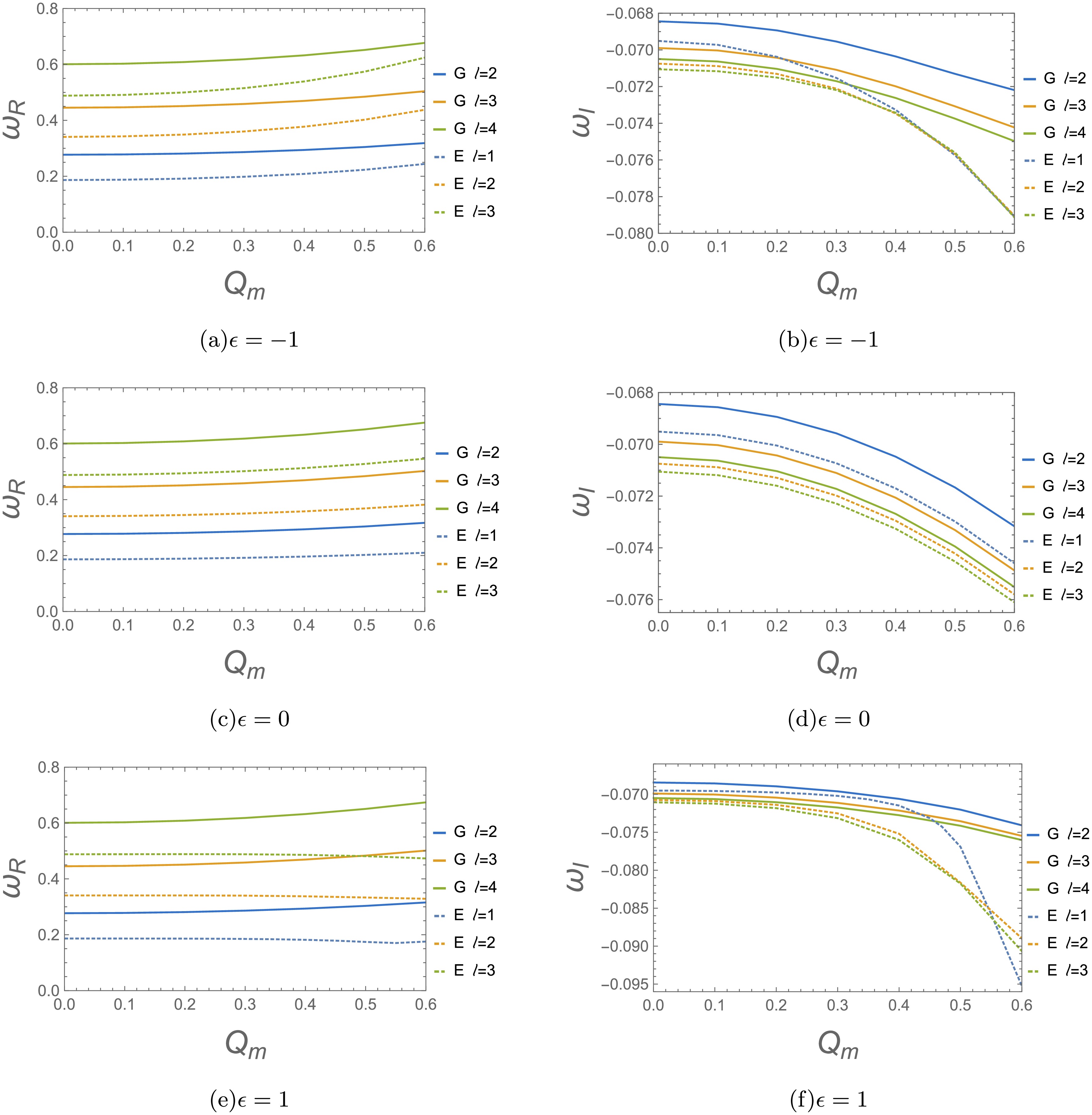

Figure 7.  (color online) Variation in the fundamental gravitational and electromagnetic quasinormal frequencies ($ n=0 $) with the magnetic charge $ Q_{\mathrm{m}} $ for a black hole with fixed mass $ M=1 $ and cosmological constant $ \Lambda=0.05 $. Panels (a) and (b) correspond to $ \epsilon=-1 $, panels (c) and (d) to $ \epsilon=0 $, and panels (e) and (f) to $ \epsilon=1 $. In each panel, the solid lines denote gravitational perturbations with $ l=2,3,4 $, whereas the dashed lines denote electromagnetic perturbations with $ l=1,2,3 $. The real and imaginary parts generally increase with increasing $ Q_{\mathrm{m}} $, except for the anomalous electromagnetic branch for $ \epsilon=1 $.

For the electromagnetic perturbation with $ \epsilon=1 $, the damping rate $ |\operatorname{Im}(\omega)| $ increases sharply as $ Q_{\text{m}} $ increases, appearing as the steep drop of the blue dashed curve in Fig. 7(f). This behavior has the same origin as the anomalous trajectory in Fig. 8(c). As shown in Fig. 5(c), for $ \epsilon=1 $, the nonlinear coupling anomalously suppresses the effective potential barrier as $ Q_{\text{m}} $ increases, in contrast to the $ \epsilon\le 0 $ cases, where the barrier becomes higher. The lowered barrier can no longer confine the electromagnetic mode efficiently, and its energy therefore leaks away rapidly, causing the damping rate to increase sharply.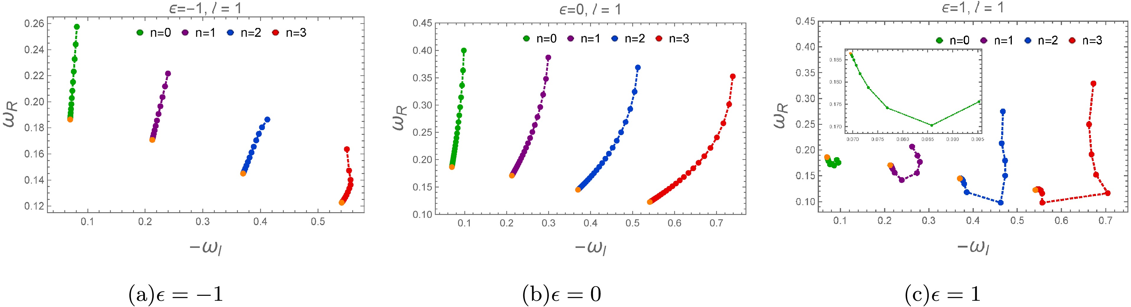

Figure 8.  (color online) Behavior of the real and imaginary parts of the quasinormal frequencies under electromagnetic perturbations for varying magnetic charge $ Q_{\text{m}} $. The parameters are fixed at $ l=1 $, $ M=1 $, and $ \Lambda=0.05 $. The orange points denote $ Q_{\text{m}}=0 $, corresponding to the uncharged Schwarzschild-de Sitter limit. The curves in different colors represent the QNMs for different overtone numbers n.

While the magnetic charge governs the nontrivial spectral shifts described above, the response of the QNMs to the remaining background parameters follows standard monotonic trends. We therefore present these results in tabular form.

Table 2 lists the frequencies for varying cosmological constant Λ. Across all branches ($ \epsilon = 0, \pm 1 $), both $ \operatorname{Re}(\omega) $ and $ |\operatorname{Im}(\omega)| $ decrease steadily as Λ increases. This slower oscillation and extended mode lifetime can be understood geometrically: increasing Λ reduces the spatial cavity between the event horizon $ r_h $ and the cosmological horizon $ r_c $, effectively creating a tighter resonant waveguide that favors lower-frequency, longer-lived modes.

Similarly, Table 3 summarizes the influence of the multipole number l. As is typical for black hole perturbations, $ \operatorname{Re}(\omega) $ increases substantially with l, whereas the damping rate $ |\operatorname{Im}(\omega)| $ exhibits only a marginal increase. This reflects the familiar physics of the centrifugal barrier: higher angular momentum raises the effective potential height, thereby increasing the oscillation frequency while leaving the decay timescale largely unaffected.

To further illustrate the spectral properties in the complex frequency plane, we plot the trajectories of the real ($ \omega_R $) and imaginary ($ -\omega_I $) parts of the quasinormal frequencies in Figs. 8 and 9. Figure 8 shows the electromagnetic sector ($ l=1 $), while Fig. 9 depicts the gravitational sector ($ l=2 $). Both figures present the evolution of the modes as the magnetic charge $ Q_{\text{m}} $ varies continuously. For all branches of $ \epsilon $ and different overtone numbers ($ n=0, 1, 2, 3 $), the variation in $ Q_{\text{m}} $ induces a clear migration of the frequencies. Notably, as $ Q_{\text{m}} \to 0 $ (indicated by the orange points), all curves smoothly converge to the uncharged Schwarzschild-de Sitter (SdS) limit, confirming the consistency of our numerical framework. Furthermore, it is evident that higher overtones (larger n) generally correspond to significantly larger damping rates ($ -\omega_I $), while their oscillation frequencies ($ \omega_R $) remain relatively clustered.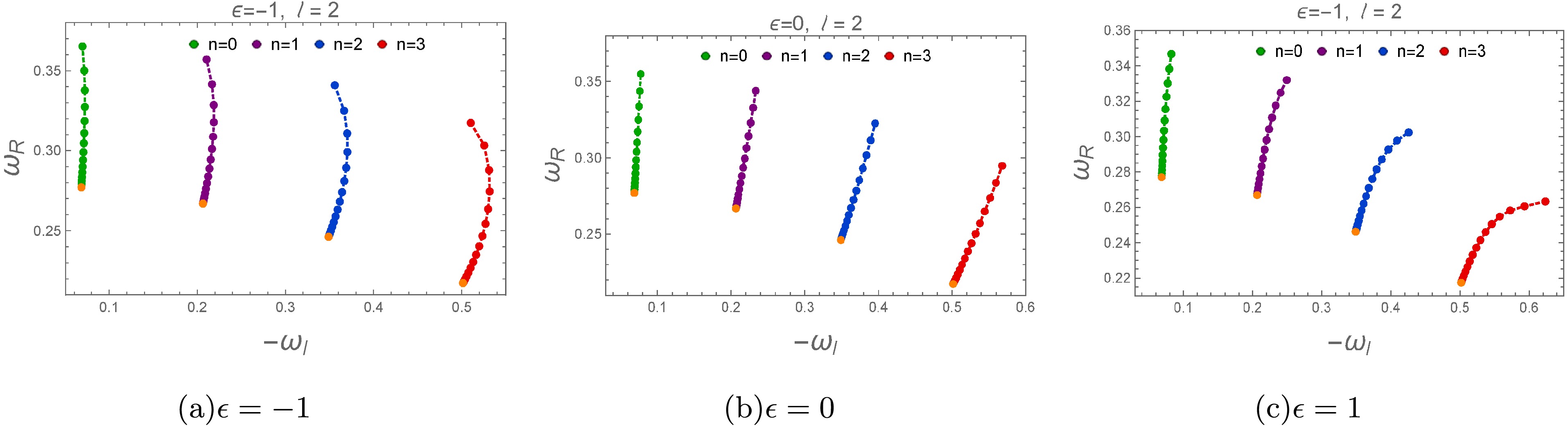

Figure 9.  (color online) Behavior of the real and imaginary parts of the quasinormal frequencies under gravitational perturbations for varying magnetic charge $ Q_{\text{m}} \in [0, 0.6] $. The parameters are set to $ l=2 $, $ M=1 $, and $ \Lambda=0.05 $. The orange points denote $ Q_{\text{m}}=0 $, corresponding to the limit in which the spacetime reduces to an uncharged Schwarzschild-de Sitter black hole. The curves in different colors represent the QNMs for different overtone numbers n.

A particularly interesting feature emerges in the electromagnetic sector for $ \epsilon = 1 $, as depicted in Fig. 8(c). Unlike the monotonic or smoothly curved trajectories observed in other parameter regimes, the QNM curves in Fig. 8(c) exhibit a highly anomalous topological shape, bending irregularly as $ Q_{\text{m}} $ increases. This distinct spectral behavior in the complex plane is closely intertwined with the underlying background geometry. Referring back to the effective potential for the electromagnetic perturbation in Fig. 5(c), one can observe that the behavior of the peak of the potential barrier under variations in $ Q_{\text{m}} $ deviates significantly from the patterns seen in Figs. 5(a) and 5(b). The anomalous suppression and shift of the potential barrier directly alter the scattering cavity, thereby manifesting as the unconventional frequency trajectories observed in Fig. 8(c). This correspondence highlights how sensitive the ringing of the black hole is to the morphology of its effective potential under nonlinear electrodynamic corrections.

Finally, in Fig. 10, we fix the magnetic charge at $ Q_{\text{m}} = 0.1 $ to directly compare the overtone spectra ($ n = 0, 1, \dots, 5 $) of the gravitational (green curves) and electromagnetic (blue curves) perturbations. The orange points specifically highlight the fundamental modes ($ n=0 $). The results show that as the overtone number n increases, the damping rate $ -\omega_I $ increases almost linearly for both fields, indicating that higher-order modes dissipate much more rapidly. Meanwhile, the real part $ \omega_R $ gradually decreases. Under the given parameters, the gravitational perturbations exhibit higher oscillation frequencies but lower damping rates than the electromagnetic perturbations. Furthermore, the overall topological structure of the overtone spectra remains robust across different nonlinear coupling parameters ($ \epsilon = -1, 0, 1 $), implying that the hierarchy of the overtones is governed primarily by the intrinsic properties of the black hole rather than by the specific details of the nonlinear electrodynamic coupling.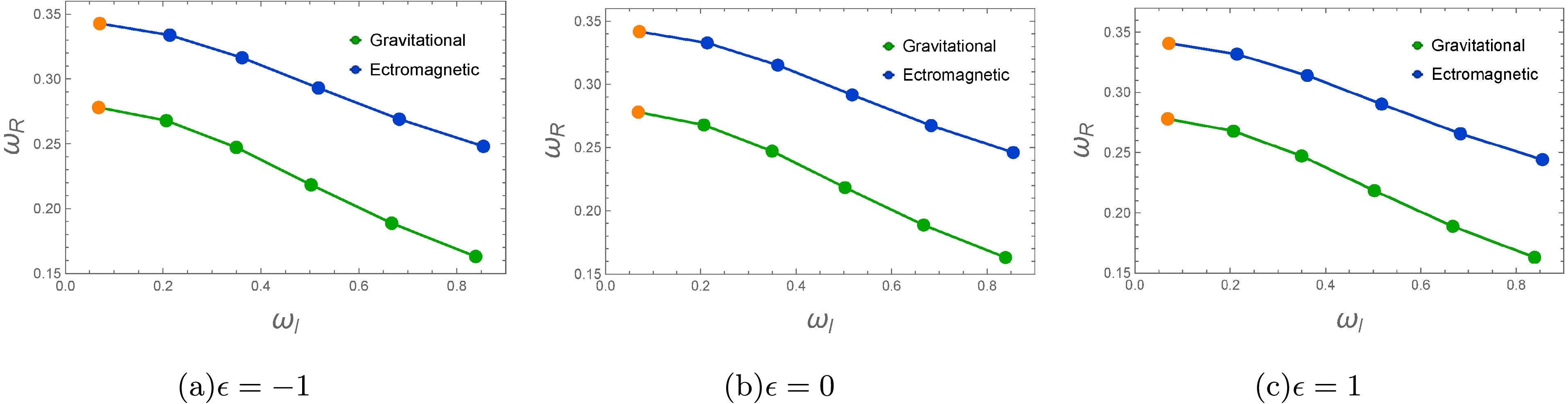

Figure 10.  (color online) Quasinormal frequencies in the complex plane for different overtone numbers n ($ n=0,1,\dots,5 $). The green curves denote gravitational perturbations with $ l=2 $, whereas the blue curves denote electromagnetic perturbations with $ l=1 $. The orange points specifically indicate the fundamental modes ($ n=0 $). Panels (a), (b), and (c) correspond to $ \epsilon=-1 $, $ \epsilon=0 $, and $ \epsilon=1 $, respectively. In all cases, the parameters are set to $ M=1 $, $ Q_{\text{m}}=0.1 $, and $ \Lambda=0.05 $.

In this section, we extend our analysis to the greybody factors of the magnetically charged dS black hole. The greybody factor quantifies the scattering properties of the spacetime's effective potential and represents the probability that an incoming wave from the cosmological horizon can tunnel through the potential barrier and be absorbed by the black hole. In the static region of de Sitter spacetime, the scattering problem is defined between the black-hole event horizon and the cosmological horizon. The appropriate boundary conditions for this scenario are defined as:

where $ T(\omega) $ and $ R(\omega) $ denote the transmission and reflection coefficients, respectively.

The squared amplitude of the wave function corresponds to the probability density. When incident waves encounter the effective potential barrier, they split into reflected and transmitted components. The transmission coefficient, $ |T(\omega)|^2 $, represents the fraction of the wave that successfully penetrates the barrier and is conventionally referred to as the greybody factor. By conservation of probability, $ R(\omega) $ and $ T(\omega) $ satisfy the relation:

To compute these coefficients, we employ the sixth-order WKB approximation, which is highly reliable for evaluating quantum tunneling through potential barriers. The reflection and transmission probabilities are given by:

where the parameter $ K(\omega) $ is determined using the WKB formula:

For more detailed derivations and applications of this method, readers may refer to reviews such as [28, 30–34] and the references therein.

In Figs. 11 and 12, we present the frequency-dependent greybody factors $ |T(\omega)|^2 $ for gravitational ($ l=2 $) and electromagnetic ($ l=1 $) perturbations, respectively, for varying magnetic charge $ Q_{\text{m}} $. For gravitational perturbations, and for electromagnetic perturbations with $ \epsilon\le 0 $, increasing the magnetic charge $ Q_{\text{m}} $ shifts the transmission curve to the right and decreases the greybody factor at a fixed frequency. In these cases, a larger magnetic charge increases both the height and width of the effective potential barrier, requiring higher incident-wave frequencies to overcome it. The electromagnetic perturbation with $ \epsilon=1 $ is an exception and is discussed below.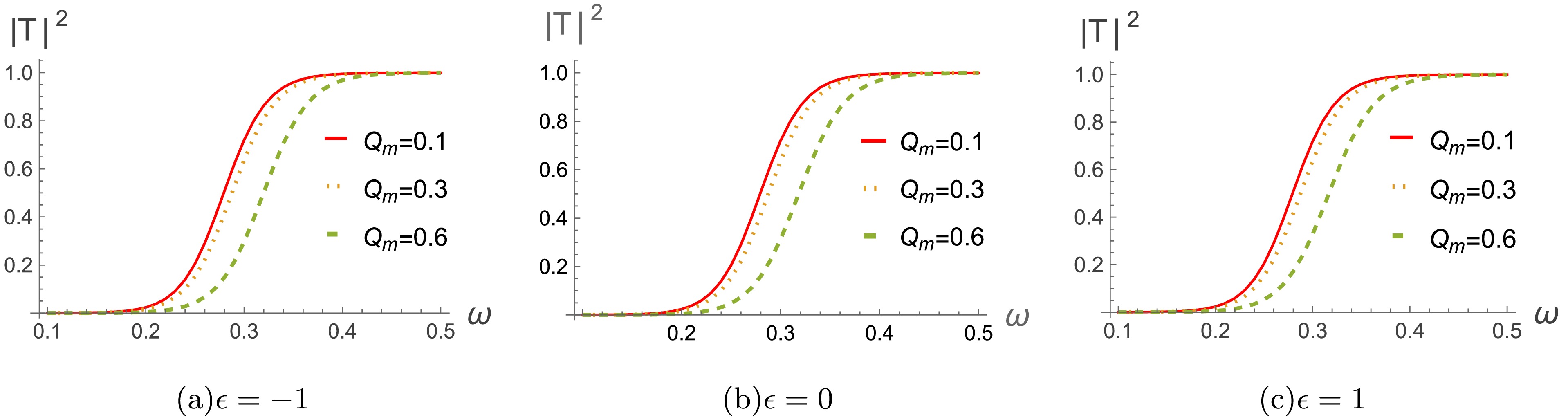

Figure 11.  (color online) The greybody factors for the gravitational field with $ M = 1 $, $ \Lambda = 0.05 $, and $ l = 2 $.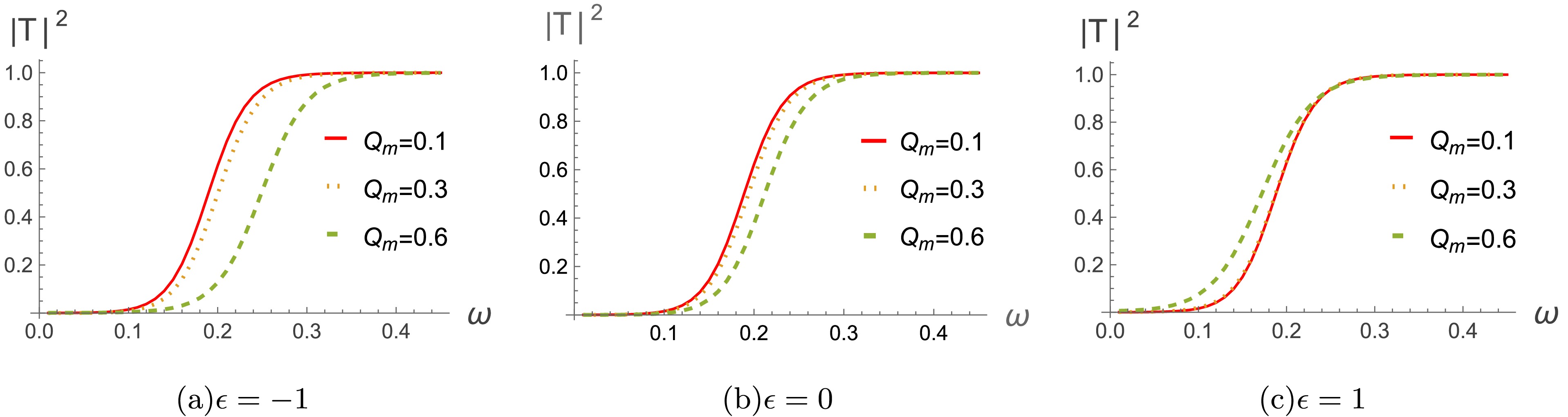

Figure 12.  (color online) The greybody factors for the electromagnetic field with $ M=1 $, $ \Lambda=0.05 $, and $ l=1 $.

For the electromagnetic perturbation with $ \epsilon=1 $ (Fig. 12(c)), the transmission curves are not nested in the same regular order as in the other panels. This is consistent with our QNM analysis and originates from the behavior of the effective potential barrier shown in Fig. 5(c). For $ \epsilon\le 0 $, increasing $ Q_{\text{m}} $ raises the barrier, so the wave tunnels less easily and the transmission curve shifts to the right in a regular manner. By contrast, at $ \epsilon=1 $, the barrier is anomalously suppressed as $ Q_{\text{m}} $ increases, making tunnelling easier rather than harder. The transmission curve for the largest $ Q_{\text{m}} $ therefore breaks the ordered right-shifting pattern and lies outside the main distribution.

Furthermore, we investigate the influence of the multipole number l on the greybody factors, with the results for gravitational and electromagnetic fields shown in Figs. 13 and 14, respectively. It is evident that the transmission probability decreases drastically as l increases. This phenomenon is rooted in the structure of the effective potential: a higher multipole number corresponds to a significantly stronger centrifugal barrier in the spacetime geometry. This enhanced centrifugal barrier effectively shields the black hole, markedly reducing the tunnelling probability for modes with larger angular momentum. These scattering behaviors are in excellent agreement with the morphological evolution of the effective potentials illustrated in Figs. 4 and 6, providing a self-consistent picture of wave dynamics in this nonlinear electrodynamic background [57].

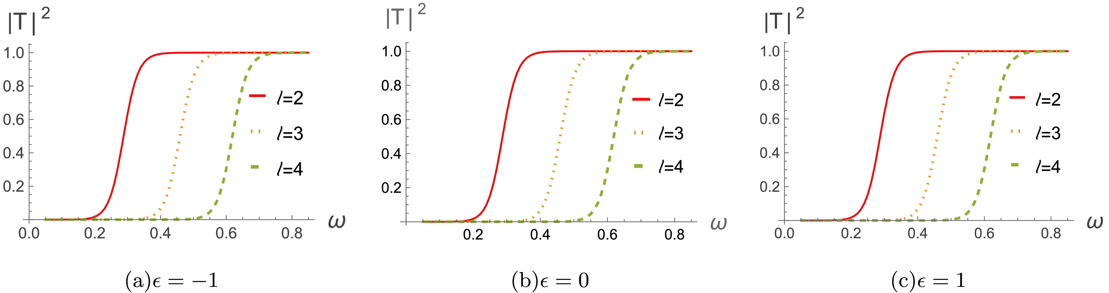
Figure 13.  (color online) The greybody factors for the gravitational field with $ M=1 $, $ Q_{\text{m}}=0.3 $, and $ \Lambda=0.05 $.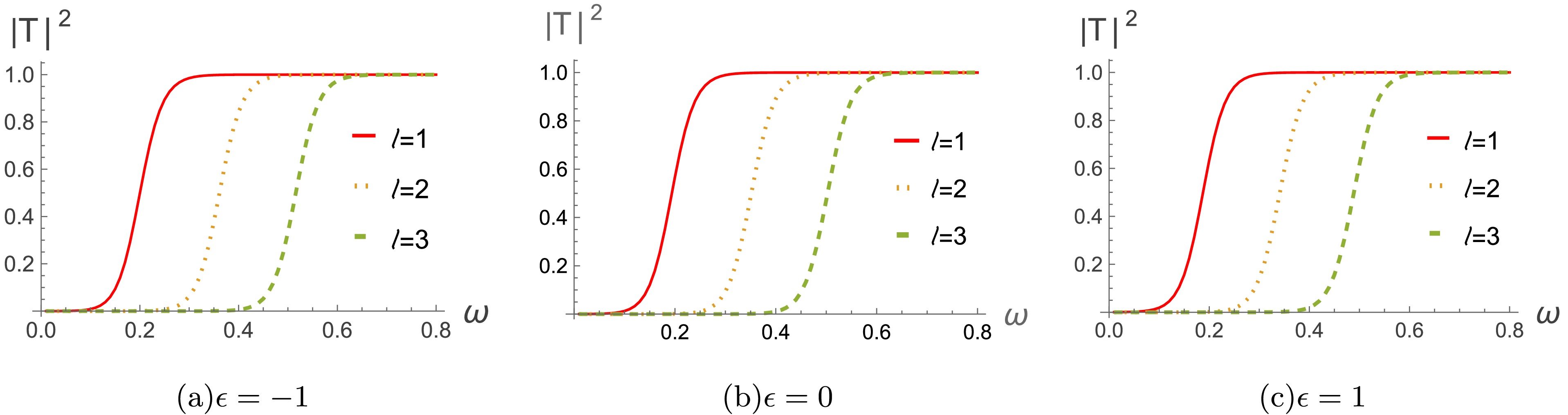

Figure 14.  (color online) The greybody factors for the electromagnetic field with $ M=1 $, $ Q_{\text{m}}=0.3 $, and $ \Lambda=0.05 $.

The greybody factor is closely related to the Hawking sparsity of black hole radiation, as discussed in Refs. [28, 29, 50, 51, 55]. A lower greybody factor indicates weaker transmission and therefore suggests sparser radiation. Thus, larger $ Q_{\text{m}} $ and l generally correspond to sparser radiation, while the electromagnetic sector with $ \epsilon=1 $ exhibits an anomalous response.

In this work, we investigated axial gravitational and electromagnetic perturbations of magnetically charged black holes in a de Sitter background within string-inspired Euler-Heisenberg gravity. A key feature of this model is that the axial metric perturbations decouple completely from the electromagnetic sector, enabling the two perturbation equations to be reduced to separate Schrödinger-like master equations. We further showed that the associated effective potentials remain positive throughout the parameter ranges considered. This supports the modal stability of the black hole under axial gravitational and electromagnetic perturbations.

Using the AIM and sixth-order WKB methods, we computed the quasinormal frequencies and found excellent numerical agreement between the two approaches. Parametric analysis reveals that a larger cosmological constant Λ produces slower, longer-lived modes, whereas higher multipole numbers l predictably increase the oscillation frequencies. Increasing the magnetic charge $ Q_{\text{m}} $ generally leads to faster oscillations and more rapid decay. Notably, in the electromagnetic sector with $ \epsilon=1 $ coupling, the frequencies exhibit anomalous, non-monotonic trajectories in the complex plane, providing a direct signature of the deformed potential barrier induced by nonlinear electrodynamics. Overtone modes behave conventionally, decaying more rapidly at higher n, with a spectral spacing that remains robust against variations in $ \epsilon $. Complementing the QNM spectra, the WKB evaluation of greybody factors shows that wave transmission is generally suppressed for larger $ Q_{\text{m}} $ or l, while the electromagnetic sector with $ \epsilon=1 $ exhibits an anomalous response associated with the deformation of the effective potential barrier.

Looking ahead, exploring polar (even-parity) perturbations, in which metric and gauge fluctuations are inherently coupled [44, 45, 46], remains an essential next step toward completing the stability profile of magnetic black holes in string-inspired Euler-Heisenberg gravity.