


 Abstract
 HTML
 Reference
 Related
 PDF



-
α decay is a major decay mode of heavy and superheavy nuclei and plays a crucial role in current research on superheavy nuclei and in the identification of new elements and nuclides. In 1899, while investigating uranium radiation, Rutherford discovered that it consisted of two distinct components: one with extremely weak penetrating power, easily absorbed by thin layers of material, which he named α rays; and the other with stronger penetrating ability, which he called β rays [1]. This marked the beginning of systematic research on α decay and represented a significant development in nuclear physics [2]. Over the following decade, Rutherford and his collaborators gradually revealed the nature of α particles [3]. By emitting α rays in discharge tubes and observing their characteristic spectrum for the first time in 1908, they ultimately confirmed that α particles are doubly ionized helium nuclei. This discovery not only revealed the phenomenon of α decay for the first time, but also laid the experimental and theoretical foundation for the concept of half-life. Later, in 1928, Gurney and Condon [2] and Gamow [4] independently proposed the quantum tunneling theory to estimate the probability of α particles tunneling through Coulomb barriers. Since then, α decay has remained an important research topic in nuclear physics. As a highly sensitive probe, it provides a key means of studying unstable, neutron-deficient, and superheavy nuclei, revealing extensive structural information such as nuclear deformation [5−7], shell effects [8, 9], and valence-nucleon dynamics [10−12].
To date, various models have been developed to describe the process of α decay, including the cluster model [13−15], the generalized liquid drop model (GLDM) [16−18], the density-dependent cluster model (DDCM) [19, 20], the two-potential approach [21−27], and the analytical superasymmetric fission (ASAF) model [28−33]. Meanwhile, a series of empirical formulae have also been developed to calculate α-decay half-lives, including the scaling law of Brown formula (SLB) [34], the universal decay law (UDL) [35, 36], the Royer formula along with its improved forms such as the modified Royer formula (MR) [37] and the unitary Royer formula (DZR) [38], the Viola-Seaborg formula (VS) [39], proposed in 1966 and later further modified into the Viola-Seaborg-Sobiczewski formula (VSS) [40] and the modified Viola-Seaborg formula (MVS) [41], the NRDX formula [42], the Hatsukawa formula [43], and others [44, 45]. These models and empirical formulae rest on two key assumptions: first, that α-particle clusters are preformed on the surface of the parent nucleus; and second, that the preformed clusters tunnel through the potential barriers. Thus, a complete understanding of α decay requires addressing two fundamental issues: the precise calculation of preformation factors and the determination of the quantum tunneling probability.
With respect to the first issue, namely the preformation factor, its role in the theoretical description of α-decay half-lives is crucial. It is not a simple computable quantity, as it contains rich structural information such as shell effects, nuclear pairing correlations, deformations, and residual interactions [18, 46]. Essentially, it is a problem involving the overlap of multiple quantum states and therefore cannot be solved strictly from first principles. In many previous studies, the α-particle preformation probability has been taken as a constant for simplicity [16, 47], estimated using an analytic formula [48], or extracted solely through phenomenological fits to experimental decay data [49, 50]. For example, within the framework of the density-dependent cluster model (DDCM), the preformation factor has commonly been taken as 0.43 for even-even nuclei [19]. Recently, Ahmed et al. proposed a new quantum-mechanical theory called the CFM [51−54] to calculate
$ P_\alpha $ , suggesting that the initial state of the parent nucleus should be a linear combination of different possible clusterization states. They successfully determined$ P_\alpha = 0.22 $ for$ ^{212}\mathrm{Po} $ using the CFM, which reproduced well the calculations of Varga et al. [55, 56]. With respect to the second issue, the calculation of the penetration probability is most commonly performed using the WKB approximation. As an alternative, the transition matrix method has been applied to α decay [57]. It can solve the penetration coefficient of the one-dimensional stationary Schrödinger equation numerically and accurately and is applicable to any shape of potential barrier.Recently, the roles of nuclear deformation and shell effects in α-decay models have attracted considerable research interest [58, 59]. Furthermore, improved theoretical formulae have been proposed to account for daughter-nucleus deformation in heavy nuclei [60], and specific studies have focused on the α and cluster decay modes of superheavy nuclei with Z = 122 [61], providing important theoretical insights into the decay pathways of these extreme systems [62−65]. In view of the above, we employ the CFM combined with the transition matrix method to calculate the α-decay half-lives of 177 even-even nuclei. A comparison between the phenomenological cosh potential and the microscopic DDM3Y double-folding potential is carried out. The quadrupole and hexadecapole deformations are incorporated through orientation averaging using FRDM parameters. In addition, we predict the half-lives of 61 even-even nuclei with proton numbers Z = 120 and 122, which may provide references for subsequent experimental work. The model parameters are obtained by fitting the α-decay half-lives of 177 even-even nuclei taken from the latest nuclear property table NUBASE2020 [66].
This article is organized as follows. In Sec. II, the theoretical framework of α-decay half-lives and preformation probabilities is briefly described. The detailed results and discussion are presented in Sec. III. Finally, a brief summary is given in Sec. IV.
-
α decay is a major decay mode of heavy and superheavy nuclei and plays a crucial role in current research on superheavy nuclei and in the identification of new elements and nuclides. In 1899, while investigating uranium radiation, Rutherford discovered that it consisted of two distinct components: one with extremely weak penetrating power, easily absorbed by thin layers of material, which he named α rays; and the other with stronger penetrating ability, which he called β rays [1]. This marked the beginning of systematic research on α decay and represented a significant development in nuclear physics [2]. Over the following decade, Rutherford and his collaborators gradually revealed the nature of α particles [3]. By emitting α rays in discharge tubes and observing their characteristic spectrum for the first time in 1908, they ultimately confirmed that α particles are doubly ionized helium nuclei. This discovery not only revealed the phenomenon of α decay for the first time, but also laid the experimental and theoretical foundation for the concept of half-life. Later, in 1928, Gurney and Condon [2] and Gamow [4] independently proposed the quantum tunneling theory to estimate the probability of α particles tunneling through Coulomb barriers. Since then, α decay has remained an important research topic in nuclear physics. As a highly sensitive probe, it provides a key means of studying unstable, neutron-deficient, and superheavy nuclei, revealing extensive structural information such as nuclear deformation [5−7], shell effects [8, 9], and valence-nucleon dynamics [10−12].
To date, various models have been developed to describe the process of α decay, including the cluster model [13−15], the generalized liquid drop model (GLDM) [16−18], the density-dependent cluster model (DDCM) [19, 20], the two-potential approach [21−27], and the analytical superasymmetric fission (ASAF) model [28−33]. Meanwhile, a series of empirical formulae have also been developed to calculate α-decay half-lives, including the scaling law of Brown formula (SLB) [34], the universal decay law (UDL) [35, 36], the Royer formula along with its improved forms such as the modified Royer formula (MR) [37] and the unitary Royer formula (DZR) [38], the Viola-Seaborg formula (VS) [39], proposed in 1966 and later further modified into the Viola-Seaborg-Sobiczewski formula (VSS) [40] and the modified Viola-Seaborg formula (MVS) [41], the NRDX formula [42], the Hatsukawa formula [43], and others [44, 45]. These models and empirical formulae rest on two key assumptions: first, that α-particle clusters are preformed on the surface of the parent nucleus; and second, that the preformed clusters tunnel through the potential barriers. Thus, a complete understanding of α decay requires addressing two fundamental issues: the precise calculation of preformation factors and the determination of the quantum tunneling probability.
With respect to the first issue, namely the preformation factor, its role in the theoretical description of α-decay half-lives is crucial. It is not a simple computable quantity, as it contains rich structural information such as shell effects, nuclear pairing correlations, deformations, and residual interactions [18, 46]. Essentially, it is a problem involving the overlap of multiple quantum states and therefore cannot be solved strictly from first principles. In many previous studies, the α-particle preformation probability has been taken as a constant for simplicity [16, 47], estimated using an analytic formula [48], or extracted solely through phenomenological fits to experimental decay data [49, 50]. For example, within the framework of the density-dependent cluster model (DDCM), the preformation factor has commonly been taken as 0.43 for even-even nuclei [19]. Recently, Ahmed et al. proposed a new quantum-mechanical theory called the CFM [51−54] to calculate
$ P_\alpha $ , suggesting that the initial state of the parent nucleus should be a linear combination of different possible clusterization states. They successfully determined$ P_\alpha = 0.22 $ for$ ^{212}\mathrm{Po} $ using the CFM, which reproduced well the calculations of Varga et al. [55, 56]. With respect to the second issue, the calculation of the penetration probability is most commonly performed using the WKB approximation. As an alternative, the transition matrix method has been applied to α decay [57]. It can solve the penetration coefficient of the one-dimensional stationary Schrödinger equation numerically and accurately and is applicable to any shape of potential barrier.Recently, the roles of nuclear deformation and shell effects in α-decay models have attracted considerable research interest [58, 59]. Furthermore, improved theoretical formulae have been proposed to account for daughter-nucleus deformation in heavy nuclei [60], and specific studies have focused on the α and cluster decay modes of superheavy nuclei with Z = 122 [61], providing important theoretical insights into the decay pathways of these extreme systems [62−65]. In view of the above, we employ the CFM combined with the transition matrix method to calculate the α-decay half-lives of 177 even-even nuclei. A comparison between the phenomenological cosh potential and the microscopic DDM3Y double-folding potential is carried out. The quadrupole and hexadecapole deformations are incorporated through orientation averaging using FRDM parameters. In addition, we predict the half-lives of 61 even-even nuclei with proton numbers Z = 120 and 122, which may provide references for subsequent experimental work. The model parameters are obtained by fitting the α-decay half-lives of 177 even-even nuclei taken from the latest nuclear property table NUBASE2020 [66].
This article is organized as follows. In Sec. II, the theoretical framework of α-decay half-lives and preformation probabilities is briefly described. The detailed results and discussion are presented in Sec. III. Finally, a brief summary is given in Sec. IV.
-
α decay is a major decay mode of heavy and superheavy nuclei and plays a crucial role in current research on superheavy nuclei and in the identification of new elements and nuclides. In 1899, while investigating uranium radiation, Rutherford discovered that it consisted of two distinct components: one with extremely weak penetrating power, easily absorbed by thin layers of material, which he named α rays; and the other with stronger penetrating ability, which he called β rays [1]. This marked the beginning of systematic research on α decay and represented a significant development in nuclear physics [2]. Over the following decade, Rutherford and his collaborators gradually revealed the nature of α particles [3]. By emitting α rays in discharge tubes and observing their characteristic spectrum for the first time in 1908, they ultimately confirmed that α particles are doubly ionized helium nuclei. This discovery not only revealed the phenomenon of α decay for the first time, but also laid the experimental and theoretical foundation for the concept of half-life. Later, in 1928, Gurney and Condon [2] and Gamow [4] independently proposed the quantum tunneling theory to estimate the probability of α particles tunneling through Coulomb barriers. Since then, α decay has remained an important research topic in nuclear physics. As a highly sensitive probe, it provides a key means of studying unstable, neutron-deficient, and superheavy nuclei, revealing extensive structural information such as nuclear deformation [5−7], shell effects [8, 9], and valence-nucleon dynamics [10−12].
To date, various models have been developed to describe the process of α decay, including the cluster model [13−15], the generalized liquid drop model (GLDM) [16−18], the density-dependent cluster model (DDCM) [19, 20], the two-potential approach [21−27], and the analytical superasymmetric fission (ASAF) model [28−33]. Meanwhile, a series of empirical formulae have also been developed to calculate α-decay half-lives, including the scaling law of Brown formula (SLB) [34], the universal decay law (UDL) [35, 36], the Royer formula along with its improved forms such as the modified Royer formula (MR) [37] and the unitary Royer formula (DZR) [38], the Viola-Seaborg formula (VS) [39], proposed in 1966 and later further modified into the Viola-Seaborg-Sobiczewski formula (VSS) [40] and the modified Viola-Seaborg formula (MVS) [41], the NRDX formula [42], the Hatsukawa formula [43], and others [44, 45]. These models and empirical formulae rest on two key assumptions: first, that α-particle clusters are preformed on the surface of the parent nucleus; and second, that the preformed clusters tunnel through the potential barriers. Thus, a complete understanding of α decay requires addressing two fundamental issues: the precise calculation of preformation factors and the determination of the quantum tunneling probability.
With respect to the first issue, namely the preformation factor, its role in the theoretical description of α-decay half-lives is crucial. It is not a simple computable quantity, as it contains rich structural information such as shell effects, nuclear pairing correlations, deformations, and residual interactions [18, 46]. Essentially, it is a problem involving the overlap of multiple quantum states and therefore cannot be solved strictly from first principles. In many previous studies, the α-particle preformation probability has been taken as a constant for simplicity [16, 47], estimated using an analytic formula [48], or extracted solely through phenomenological fits to experimental decay data [49, 50]. For example, within the framework of the density-dependent cluster model (DDCM), the preformation factor has commonly been taken as 0.43 for even-even nuclei [19]. Recently, Ahmed et al. proposed a new quantum-mechanical theory called the CFM [51−54] to calculate
$ P_\alpha $ , suggesting that the initial state of the parent nucleus should be a linear combination of different possible clusterization states. They successfully determined$ P_\alpha = 0.22 $ for$ ^{212}\mathrm{Po} $ using the CFM, which reproduced well the calculations of Varga et al. [55, 56]. With respect to the second issue, the calculation of the penetration probability is most commonly performed using the WKB approximation. As an alternative, the transition matrix method has been applied to α decay [57]. It can solve the penetration coefficient of the one-dimensional stationary Schrödinger equation numerically and accurately and is applicable to any shape of potential barrier.Recently, the roles of nuclear deformation and shell effects in α-decay models have attracted considerable research interest [58, 59]. Furthermore, improved theoretical formulae have been proposed to account for daughter-nucleus deformation in heavy nuclei [60], and specific studies have focused on the α and cluster decay modes of superheavy nuclei with Z = 122 [61], providing important theoretical insights into the decay pathways of these extreme systems [62−65]. In view of the above, we employ the CFM combined with the transition matrix method to calculate the α-decay half-lives of 177 even-even nuclei. A comparison between the phenomenological cosh potential and the microscopic DDM3Y double-folding potential is carried out. The quadrupole and hexadecapole deformations are incorporated through orientation averaging using FRDM parameters. In addition, we predict the half-lives of 61 even-even nuclei with proton numbers Z = 120 and 122, which may provide references for subsequent experimental work. The model parameters are obtained by fitting the α-decay half-lives of 177 even-even nuclei taken from the latest nuclear property table NUBASE2020 [66].
This article is organized as follows. In Sec. II, the theoretical framework of α-decay half-lives and preformation probabilities is briefly described. The detailed results and discussion are presented in Sec. III. Finally, a brief summary is given in Sec. IV.
-
The α-decay half-life is determined by the decay constant λ. It can be expressed as
$ T_{1/2} = \frac{\ln 2}{\lambda}, $
(1) where λ is defined as
$ \lambda = P_{\alpha} v_0 P. $
(2) Here, P and
$ P_{\alpha} $ denote the penetration probability and the preformation factor, respectively, in α decay. The method used to obtain their values is described in detail in the next section.As a spherical baseline,
$ v_0 $ represents the assault frequency, which can be described as$ v_0 = \frac{1}{2R} \sqrt{\frac{2E_\alpha}{M}},$
(3) where
$ E_\alpha $ and M are the kinetic energy and mass of the α particle, respectively. The sharp radius R of the nuclear potential is calculated using an empirical formula in terms of the mass number A of the parent nucleus. It can be expressed as [18]$ R = 1.28A^{1/3} - 0.76 + 0.8A^{-1/3}. $
(4) The α-core potential
$ V(r) $ plays a crucial role in determining P. It consists of the nuclear potential$ V_N(r) $ , the Coulomb potential$ V_C(r) $ , and the centrifugal potential$ V_l(r) $ , and can be expressed as$ V(r) = V_N(r) + V_C(r) + V_l(r). $
(5) The specific forms of the nuclear potential
$V_N(r)$ and Coulomb potential$V_C(r)$ are presented in Subsection D. The potential$V_l(r)$ [67] is expressed as$ V_{\ell}(r) = \frac{\ell(\ell+1)\hbar^2}{2\mu r^2}. $
(6) Here, l is the orbital angular momentum of the α particle, and
$ \hbar $ is the reduced Planck constant.The above expressions correspond to the spherical baseline. In the present calculation, we incorporate the deformation effects of the daughter nucleus. Following the orientation treatment in Ref. [65], the emitted α particle is treated as spherical, while the daughter nucleus is assumed to have an axially symmetric intrinsic shape. The quadrupole and hexadecapole deformations are included in the calculation. The orientation-dependent radius of the daughter nucleus is expressed as
$ R(\theta) = R_{0} \left[ 1 + \sum\limits_{\lambda=2,4} \beta_{\lambda}Y_{\lambda0}(\theta) \right], $
(7) where
$ R_{0} $ is the spherical reference radius, θ is the angle between the symmetry axis and the α-emission direction, and$Y_{\lambda0}(\theta)$ denotes the real spherical harmonics. The quantities$\beta_2$ and$\beta_4$ are the quadrupole and hexadecapole deformation parameters, respectively.When the deformation of the daughter nucleus is taken into account, the radius in the assault frequency becomes orientation dependent and is given by
$ v_0(\theta) = \frac{1}{2R(\theta)} \sqrt{\frac{2E_\alpha}{M}}, $
(8) where the orientation-dependent sharp radius
$R(\theta)$ follows the same deformation expansion described above. Similarly, because the total interaction potential$V(r,\theta)$ depends on the emission orientation, the penetration probability calculated using the transition matrix method (TMM) is also angle-dependent and is denoted by$P(\theta)$ . The effective decay constant is then obtained by averaging the product$v_0(\theta)P(\theta)$ over all orientations, and is given by$ \lambda=P_{\alpha}\frac{1}{2}\int_0^{\pi}v_0(\theta)P(\theta)\sin\theta\, \mathrm{d}\theta. $
(9) -
The α-decay half-life is determined by the decay constant λ. It can be expressed as
$ T_{1/2} = \frac{\ln 2}{\lambda}, $
(1) where λ is defined as
$ \lambda = P_{\alpha} v_0 P. $
(2) Here, P and
$ P_{\alpha} $ denote the penetration probability and the preformation factor, respectively, in α decay. The method used to obtain their values is described in detail in the next section.As a spherical baseline,
$ v_0 $ represents the assault frequency, which can be described as$ v_0 = \frac{1}{2R} \sqrt{\frac{2E_\alpha}{M}},$
(3) where
$ E_\alpha $ and M are the kinetic energy and mass of the α particle, respectively. The sharp radius R of the nuclear potential is calculated using an empirical formula in terms of the mass number A of the parent nucleus. It can be expressed as [18]$ R = 1.28A^{1/3} - 0.76 + 0.8A^{-1/3}. $
(4) The α-core potential
$ V(r) $ plays a crucial role in determining P. It consists of the nuclear potential$ V_N(r) $ , the Coulomb potential$ V_C(r) $ , and the centrifugal potential$ V_l(r) $ , and can be expressed as$ V(r) = V_N(r) + V_C(r) + V_l(r). $
(5) The specific forms of the nuclear potential
$V_N(r)$ and Coulomb potential$V_C(r)$ are presented in Subsection D. The potential$V_l(r)$ [67] is expressed as$ V_{\ell}(r) = \frac{\ell(\ell+1)\hbar^2}{2\mu r^2}. $
(6) Here, l is the orbital angular momentum of the α particle, and
$ \hbar $ is the reduced Planck constant.The above expressions correspond to the spherical baseline. In the present calculation, we incorporate the deformation effects of the daughter nucleus. Following the orientation treatment in Ref. [65], the emitted α particle is treated as spherical, while the daughter nucleus is assumed to have an axially symmetric intrinsic shape. The quadrupole and hexadecapole deformations are included in the calculation. The orientation-dependent radius of the daughter nucleus is expressed as
$ R(\theta) = R_{0} \left[ 1 + \sum\limits_{\lambda=2,4} \beta_{\lambda}Y_{\lambda0}(\theta) \right], $
(7) where
$ R_{0} $ is the spherical reference radius, θ is the angle between the symmetry axis and the α-emission direction, and$Y_{\lambda0}(\theta)$ denotes the real spherical harmonics. The quantities$\beta_2$ and$\beta_4$ are the quadrupole and hexadecapole deformation parameters, respectively.When the deformation of the daughter nucleus is taken into account, the radius in the assault frequency becomes orientation dependent and is given by
$ v_0(\theta) = \frac{1}{2R(\theta)} \sqrt{\frac{2E_\alpha}{M}}, $
(8) where the orientation-dependent sharp radius
$R(\theta)$ follows the same deformation expansion described above. Similarly, because the total interaction potential$V(r,\theta)$ depends on the emission orientation, the penetration probability calculated using the transition matrix method (TMM) is also angle-dependent and is denoted by$P(\theta)$ . The effective decay constant is then obtained by averaging the product$v_0(\theta)P(\theta)$ over all orientations, and is given by$ \lambda=P_{\alpha}\frac{1}{2}\int_0^{\pi}v_0(\theta)P(\theta)\sin\theta\, \mathrm{d}\theta. $
(9) -
The α-decay half-life is determined by the decay constant λ. It can be expressed as
$ T_{1/2} = \frac{\ln 2}{\lambda}, $
(1) where λ is defined as
$ \lambda = P_{\alpha} v_0 P. $
(2) Here, P and
$ P_{\alpha} $ denote the penetration probability and the preformation factor, respectively, in α decay. The method used to obtain their values is described in detail in the next section.As a spherical baseline,
$ v_0 $ represents the assault frequency, which can be described as$ v_0 = \frac{1}{2R} \sqrt{\frac{2E_\alpha}{M}},$
(3) where
$ E_\alpha $ and M are the kinetic energy and mass of the α particle, respectively. The sharp radius R of the nuclear potential is calculated using an empirical formula in terms of the mass number A of the parent nucleus. It can be expressed as [18]$ R = 1.28A^{1/3} - 0.76 + 0.8A^{-1/3}. $
(4) The α-core potential
$ V(r) $ plays a crucial role in determining P. It consists of the nuclear potential$ V_N(r) $ , the Coulomb potential$ V_C(r) $ , and the centrifugal potential$ V_l(r) $ , and can be expressed as$ V(r) = V_N(r) + V_C(r) + V_l(r). $
(5) The specific forms of the nuclear potential
$V_N(r)$ and Coulomb potential$V_C(r)$ are presented in Subsection D. The potential$V_l(r)$ [67] is expressed as$ V_{\ell}(r) = \frac{\ell(\ell+1)\hbar^2}{2\mu r^2}. $
(6) Here, l is the orbital angular momentum of the α particle, and
$ \hbar $ is the reduced Planck constant.The above expressions correspond to the spherical baseline. In the present calculation, we incorporate the deformation effects of the daughter nucleus. Following the orientation treatment in Ref. [65], the emitted α particle is treated as spherical, while the daughter nucleus is assumed to have an axially symmetric intrinsic shape. The quadrupole and hexadecapole deformations are included in the calculation. The orientation-dependent radius of the daughter nucleus is expressed as
$ R(\theta) = R_{0} \left[ 1 + \sum\limits_{\lambda=2,4} \beta_{\lambda}Y_{\lambda0}(\theta) \right], $
(7) where
$ R_{0} $ is the spherical reference radius, θ is the angle between the symmetry axis and the α-emission direction, and$Y_{\lambda0}(\theta)$ denotes the real spherical harmonics. The quantities$\beta_2$ and$\beta_4$ are the quadrupole and hexadecapole deformation parameters, respectively.When the deformation of the daughter nucleus is taken into account, the radius in the assault frequency becomes orientation dependent and is given by
$ v_0(\theta) = \frac{1}{2R(\theta)} \sqrt{\frac{2E_\alpha}{M}}, $
(8) where the orientation-dependent sharp radius
$R(\theta)$ follows the same deformation expansion described above. Similarly, because the total interaction potential$V(r,\theta)$ depends on the emission orientation, the penetration probability calculated using the transition matrix method (TMM) is also angle-dependent and is denoted by$P(\theta)$ . The effective decay constant is then obtained by averaging the product$v_0(\theta)P(\theta)$ over all orientations, and is given by$ \lambda=P_{\alpha}\frac{1}{2}\int_0^{\pi}v_0(\theta)P(\theta)\sin\theta\, \mathrm{d}\theta. $
(9) -
Within the framework of the CFM [51−54], the total clusterization state Ψ of the parent nucleus is treated as a linear combination of its n possible clusterization states
$ \Psi_i $ , indexed by i. This can be expressed as$ \Psi = \sum\limits_{i=1}^{n} a_i \Psi_i, $
(10) $ a_i=\int_{ }^{ }\Psi_i^*\Psi\, \mathrm{d}\tau, $
(11) where
$ a_i $ denotes the superposition coefficient of$ \Psi_i $ , based on the orthogonality condition$ \sum\limits_{i=1}^{n} |a_i|^2 = 1. $
(12) The total wave function is an eigenfunction of the total Hamiltonian H. Likewise, H can be written as
$ H = \sum\limits_{i=1}^{n} H_i, $
(13) with
$ H_i $ denoting the Hamiltonian for the i-th clusterization state$ \Psi_i $ . Because all clusterizations describe the same nucleus, they are assumed to share the same total energy E of the total wave function. Accordingly, the total energy E can be expressed as$ E = \sum\limits_{i=1}^{n} |a_i|^2 E = \sum\limits_{i=1}^{n} E_{fi}. $
(14) Here,
$ E_{fi} $ denotes the formation energy of the cluster in the i-th clusterization state$ \Psi_i $ . Thus, the α preformation factor is defined as$ P_\alpha = |a_\alpha|^2 = \frac{E_{f\alpha}}{E}, $
(15) where
$ a_\alpha $ denotes the coefficient of the α-clusterization state.$ E_{f\alpha} $ is the formation energy of the α cluster. E consists of$ E_{f\alpha} $ and the interaction energy between the α cluster and the daughter nucleus. Within the CFM [51−54], the values of the α-cluster formation energy$ E_{f\alpha} $ and the total energy E of the system depend on the type of parent nucleus. The corresponding formulae are classified into the following four cases:Case I: even-even nuclei,
$ \begin{aligned}[b] E_{f\alpha} =& 3B(A,Z) + B(A-4,Z-2) \\ &- 2B(A-1,Z-1) - 2B(A-1,Z), \end{aligned} $
(16a) $ E = B(A,Z) - B(A-4,Z-2); $
(16b) Case II: even Z-odd N, i.e., even-odd nuclei,
$ \begin{aligned}[b] E_{f\alpha} = &3B(A-1,Z) + B(A-5,Z-2) \\ & - 2B(A-2,Z-1) - 2B(A-2,Z), \end{aligned} $
(17a) $ E = B(A,Z) - B(A-5,Z-2); $
(17b) Case III: odd-Z, even-N nuclei, i.e., odd-even nuclei,
$ \begin{aligned}[b] E_{f\alpha} =& 3B(A-1,Z-1) + B(A-5,Z-3) \\ &- 2B(A-2,Z-2) - 2B(A-2,Z-1), \end{aligned} $
(18a) $ E = B(A,Z) - B(A-5,Z-3); $
(18b) Case IV: doubly odd nuclei,
$ \begin{aligned}[b] E_{f\alpha} = &3B(A-2,Z-1) + B(A-6,Z-3) \\& - 2B(A-3,Z-2) - 2B(A-3,Z-1), \end{aligned} $
(19a) $ E = B(A,Z) - B(A-6,Z-3), $
(19b) where
$ B(A,Z) $ denotes the binding energy of a nucleus with mass number A and proton number Z. -
Within the framework of the CFM [51−54], the total clusterization state Ψ of the parent nucleus is treated as a linear combination of its n possible clusterization states
$ \Psi_i $ , indexed by i. This can be expressed as$ \Psi = \sum\limits_{i=1}^{n} a_i \Psi_i, $
(10) $ a_i=\int_{ }^{ }\Psi_i^*\Psi\, \mathrm{d}\tau, $
(11) where
$ a_i $ denotes the superposition coefficient of$ \Psi_i $ , based on the orthogonality condition$ \sum\limits_{i=1}^{n} |a_i|^2 = 1. $
(12) The total wave function is an eigenfunction of the total Hamiltonian H. Likewise, H can be written as
$ H = \sum\limits_{i=1}^{n} H_i, $
(13) with
$ H_i $ denoting the Hamiltonian for the i-th clusterization state$ \Psi_i $ . Because all clusterizations describe the same nucleus, they are assumed to share the same total energy E of the total wave function. Accordingly, the total energy E can be expressed as$ E = \sum\limits_{i=1}^{n} |a_i|^2 E = \sum\limits_{i=1}^{n} E_{fi}. $
(14) Here,
$ E_{fi} $ denotes the formation energy of the cluster in the i-th clusterization state$ \Psi_i $ . Thus, the α preformation factor is defined as$ P_\alpha = |a_\alpha|^2 = \frac{E_{f\alpha}}{E}, $
(15) where
$ a_\alpha $ denotes the coefficient of the α-clusterization state.$ E_{f\alpha} $ is the formation energy of the α cluster. E consists of$ E_{f\alpha} $ and the interaction energy between the α cluster and the daughter nucleus. Within the CFM [51−54], the values of the α-cluster formation energy$ E_{f\alpha} $ and the total energy E of the system depend on the type of parent nucleus. The corresponding formulae are classified into the following four cases:Case I: even-even nuclei,
$ \begin{aligned}[b] E_{f\alpha} =& 3B(A,Z) + B(A-4,Z-2) \\ &- 2B(A-1,Z-1) - 2B(A-1,Z), \end{aligned} $
(16a) $ E = B(A,Z) - B(A-4,Z-2); $
(16b) Case II: even Z-odd N, i.e., even-odd nuclei,
$ \begin{aligned}[b] E_{f\alpha} = &3B(A-1,Z) + B(A-5,Z-2) \\ & - 2B(A-2,Z-1) - 2B(A-2,Z), \end{aligned} $
(17a) $ E = B(A,Z) - B(A-5,Z-2); $
(17b) Case III: odd-Z, even-N nuclei, i.e., odd-even nuclei,
$ \begin{aligned}[b] E_{f\alpha} =& 3B(A-1,Z-1) + B(A-5,Z-3) \\ &- 2B(A-2,Z-2) - 2B(A-2,Z-1), \end{aligned} $
(18a) $ E = B(A,Z) - B(A-5,Z-3); $
(18b) Case IV: doubly odd nuclei,
$ \begin{aligned}[b] E_{f\alpha} = &3B(A-2,Z-1) + B(A-6,Z-3) \\& - 2B(A-3,Z-2) - 2B(A-3,Z-1), \end{aligned} $
(19a) $ E = B(A,Z) - B(A-6,Z-3), $
(19b) where
$ B(A,Z) $ denotes the binding energy of a nucleus with mass number A and proton number Z. -
Within the framework of the CFM [51−54], the total clusterization state Ψ of the parent nucleus is treated as a linear combination of its n possible clusterization states
$ \Psi_i $ , indexed by i. This can be expressed as$ \Psi = \sum\limits_{i=1}^{n} a_i \Psi_i, $
(10) $ a_i=\int_{ }^{ }\Psi_i^*\Psi\, \mathrm{d}\tau, $
(11) where
$ a_i $ denotes the superposition coefficient of$ \Psi_i $ , based on the orthogonality condition$ \sum\limits_{i=1}^{n} |a_i|^2 = 1. $
(12) The total wave function is an eigenfunction of the total Hamiltonian H. Likewise, H can be written as
$ H = \sum\limits_{i=1}^{n} H_i, $
(13) with
$ H_i $ denoting the Hamiltonian for the i-th clusterization state$ \Psi_i $ . Because all clusterizations describe the same nucleus, they are assumed to share the same total energy E of the total wave function. Accordingly, the total energy E can be expressed as$ E = \sum\limits_{i=1}^{n} |a_i|^2 E = \sum\limits_{i=1}^{n} E_{fi}. $
(14) Here,
$ E_{fi} $ denotes the formation energy of the cluster in the i-th clusterization state$ \Psi_i $ . Thus, the α preformation factor is defined as$ P_\alpha = |a_\alpha|^2 = \frac{E_{f\alpha}}{E}, $
(15) where
$ a_\alpha $ denotes the coefficient of the α-clusterization state.$ E_{f\alpha} $ is the formation energy of the α cluster. E consists of$ E_{f\alpha} $ and the interaction energy between the α cluster and the daughter nucleus. Within the CFM [51−54], the values of the α-cluster formation energy$ E_{f\alpha} $ and the total energy E of the system depend on the type of parent nucleus. The corresponding formulae are classified into the following four cases:Case I: even-even nuclei,
$ \begin{aligned}[b] E_{f\alpha} =& 3B(A,Z) + B(A-4,Z-2) \\ &- 2B(A-1,Z-1) - 2B(A-1,Z), \end{aligned} $
(16a) $ E = B(A,Z) - B(A-4,Z-2); $
(16b) Case II: even Z-odd N, i.e., even-odd nuclei,
$ \begin{aligned}[b] E_{f\alpha} = &3B(A-1,Z) + B(A-5,Z-2) \\ & - 2B(A-2,Z-1) - 2B(A-2,Z), \end{aligned} $
(17a) $ E = B(A,Z) - B(A-5,Z-2); $
(17b) Case III: odd-Z, even-N nuclei, i.e., odd-even nuclei,
$ \begin{aligned}[b] E_{f\alpha} =& 3B(A-1,Z-1) + B(A-5,Z-3) \\ &- 2B(A-2,Z-2) - 2B(A-2,Z-1), \end{aligned} $
(18a) $ E = B(A,Z) - B(A-5,Z-3); $
(18b) Case IV: doubly odd nuclei,
$ \begin{aligned}[b] E_{f\alpha} = &3B(A-2,Z-1) + B(A-6,Z-3) \\& - 2B(A-3,Z-2) - 2B(A-3,Z-1), \end{aligned} $
(19a) $ E = B(A,Z) - B(A-6,Z-3), $
(19b) where
$ B(A,Z) $ denotes the binding energy of a nucleus with mass number A and proton number Z. -
To accurately calculate the penetration probability, the present work employs the transition matrix method originally developed by Ando and Itoh [68]. For a given emission direction θ, this method divides the potential barrier into N segments, and the potential energy is treated as constant within each segment [57]. In the limit of increasingly fine segmentation, this piecewise-constant representation converges to the continuously varying potential. Accordingly, the potential barrier
$ V(r) $ and effective mass$ m^*(r) $ are approximately represented by multi-step functions as$ V(r) = V_j = V[(r_{j-1} + r_j)/2], $
(20) $ m^*(r) = m_j^* = m^*[(r_{j-1} + r_j)/2], $
(21) for
$r_{j-1}< r \lt r_j$ $(j = 0,1,\ldots,N,N+1)$ ,$V_j$ denotes the piecewise constant potential energy.$m_j^* = \dfrac{m_d m_\alpha}{m_d+m_\alpha}$ denotes the reduced mass of the preformed α particle and the daughter nucleus, where$m_d$ and$m_\alpha$ are the masses of the daughter nucleus and the α particle, respectively. In our numerical calculations, the effective mass$m_j^*$ is treated as a constant equal to the reduced mass, which is a standard and widely accepted approximation in the transition matrix method for α decay.The wave function
$\psi_j$ in the j-th region, which describes an α particle with energy E moving normally through the barrier, is given by$ \psi_j(x) = A_j \exp(ik_j x) + B_j \exp(-ik_j x), $
(22) where
$ k_j = \sqrt{2m^*(E - V_j)}/\hbar. $
(23) By imposing the continuity of the wave function and its derivative at each boundary, the determination of
$ A_j $ and$ B_j $ in Eq. (22) can be reduced to a matrix multiplication involving the following$ N+1 $ ($ 2\times2 $ ) matrices:$ \begin{pmatrix} A_j \\ B_j \end{pmatrix} = \prod\limits_{l=0}^{j-1} M_l \begin{pmatrix} A_0 \\ B_0 \end{pmatrix}, $
(24) where
$ M_l = \frac{1}{2} \begin{pmatrix} (1+S_l){\rm e}^{-{\rm i}(k_{l+1}-k_l)r_l} & (1-S_l){\rm e}^{-{\rm i}(k_{l+1}+k_l)r_l} \\ (1-S_l){\rm e}^{{\rm i}(k_{l+1}+k_l)r_l} & (1+S_l){\rm e}^{{\rm i}(k_{l+1}-k_l)r_l} \end{pmatrix}, $
(25) and
$ S_l = \frac{m_{l+1}^*}{m_l^*} \cdot \frac{k_l}{k_{l+1}}. $
(26) By setting
$ A_0 = 1 $ and$ B_{N+1} = 0 $ in Eq. (22) for$ j = N + 1 $ , we can calculate the transmission amplitude$ A_{N+1} $ and the penetration probability$ P(E) $ as follows:$ A_{N+1} = \frac{m_0^*}{m_{N+1}^*} \cdot \frac{k_0}{k_{N+1}} \cdot \frac{1}{M_{22}}, $
(27) $ P(E) = \dfrac{m_0^*}{m_{N+1}^*} \cdot \dfrac{k_{N+1}}{k_0} |A_{N+1}|^2, $
(28) where
$ M = \begin{pmatrix} M_{11} & M_{12} \\ M_{21} & M_{22} \end{pmatrix} = \prod\limits_{l=0}^{N} M_l. $
(29) -
To accurately calculate the penetration probability, the present work employs the transition matrix method originally developed by Ando and Itoh [68]. For a given emission direction θ, this method divides the potential barrier into N segments, and the potential energy is treated as constant within each segment [57]. In the limit of increasingly fine segmentation, this piecewise-constant representation converges to the continuously varying potential. Accordingly, the potential barrier
$ V(r) $ and effective mass$ m^*(r) $ are approximately represented by multi-step functions as$ V(r) = V_j = V[(r_{j-1} + r_j)/2], $
(20) $ m^*(r) = m_j^* = m^*[(r_{j-1} + r_j)/2], $
(21) for
$r_{j-1}< r \lt r_j$ $(j = 0,1,\ldots,N,N+1)$ ,$V_j$ denotes the piecewise constant potential energy.$m_j^* = \dfrac{m_d m_\alpha}{m_d+m_\alpha}$ denotes the reduced mass of the preformed α particle and the daughter nucleus, where$m_d$ and$m_\alpha$ are the masses of the daughter nucleus and the α particle, respectively. In our numerical calculations, the effective mass$m_j^*$ is treated as a constant equal to the reduced mass, which is a standard and widely accepted approximation in the transition matrix method for α decay.The wave function
$\psi_j$ in the j-th region, which describes an α particle with energy E moving normally through the barrier, is given by$ \psi_j(x) = A_j \exp(ik_j x) + B_j \exp(-ik_j x), $
(22) where
$ k_j = \sqrt{2m^*(E - V_j)}/\hbar. $
(23) By imposing the continuity of the wave function and its derivative at each boundary, the determination of
$ A_j $ and$ B_j $ in Eq. (22) can be reduced to a matrix multiplication involving the following$ N+1 $ ($ 2\times2 $ ) matrices:$ \begin{pmatrix} A_j \\ B_j \end{pmatrix} = \prod\limits_{l=0}^{j-1} M_l \begin{pmatrix} A_0 \\ B_0 \end{pmatrix}, $
(24) where
$ M_l = \frac{1}{2} \begin{pmatrix} (1+S_l){\rm e}^{-{\rm i}(k_{l+1}-k_l)r_l} & (1-S_l){\rm e}^{-{\rm i}(k_{l+1}+k_l)r_l} \\ (1-S_l){\rm e}^{{\rm i}(k_{l+1}+k_l)r_l} & (1+S_l){\rm e}^{{\rm i}(k_{l+1}-k_l)r_l} \end{pmatrix}, $
(25) and
$ S_l = \frac{m_{l+1}^*}{m_l^*} \cdot \frac{k_l}{k_{l+1}}. $
(26) By setting
$ A_0 = 1 $ and$ B_{N+1} = 0 $ in Eq. (22) for$ j = N + 1 $ , we can calculate the transmission amplitude$ A_{N+1} $ and the penetration probability$ P(E) $ as follows:$ A_{N+1} = \frac{m_0^*}{m_{N+1}^*} \cdot \frac{k_0}{k_{N+1}} \cdot \frac{1}{M_{22}}, $
(27) $ P(E) = \dfrac{m_0^*}{m_{N+1}^*} \cdot \dfrac{k_{N+1}}{k_0} |A_{N+1}|^2, $
(28) where
$ M = \begin{pmatrix} M_{11} & M_{12} \\ M_{21} & M_{22} \end{pmatrix} = \prod\limits_{l=0}^{N} M_l. $
(29) -
To accurately calculate the penetration probability, the present work employs the transition matrix method originally developed by Ando and Itoh [68]. For a given emission direction θ, this method divides the potential barrier into N segments, and the potential energy is treated as constant within each segment [57]. In the limit of increasingly fine segmentation, this piecewise-constant representation converges to the continuously varying potential. Accordingly, the potential barrier
$ V(r) $ and effective mass$ m^*(r) $ are approximately represented by multi-step functions as$ V(r) = V_j = V[(r_{j-1} + r_j)/2], $
(20) $ m^*(r) = m_j^* = m^*[(r_{j-1} + r_j)/2], $
(21) for
$r_{j-1}< r \lt r_j$ $(j = 0,1,\ldots,N,N+1)$ ,$V_j$ denotes the piecewise constant potential energy.$m_j^* = \dfrac{m_d m_\alpha}{m_d+m_\alpha}$ denotes the reduced mass of the preformed α particle and the daughter nucleus, where$m_d$ and$m_\alpha$ are the masses of the daughter nucleus and the α particle, respectively. In our numerical calculations, the effective mass$m_j^*$ is treated as a constant equal to the reduced mass, which is a standard and widely accepted approximation in the transition matrix method for α decay.The wave function
$\psi_j$ in the j-th region, which describes an α particle with energy E moving normally through the barrier, is given by$ \psi_j(x) = A_j \exp(ik_j x) + B_j \exp(-ik_j x), $
(22) where
$ k_j = \sqrt{2m^*(E - V_j)}/\hbar. $
(23) By imposing the continuity of the wave function and its derivative at each boundary, the determination of
$ A_j $ and$ B_j $ in Eq. (22) can be reduced to a matrix multiplication involving the following$ N+1 $ ($ 2\times2 $ ) matrices:$ \begin{pmatrix} A_j \\ B_j \end{pmatrix} = \prod\limits_{l=0}^{j-1} M_l \begin{pmatrix} A_0 \\ B_0 \end{pmatrix}, $
(24) where
$ M_l = \frac{1}{2} \begin{pmatrix} (1+S_l){\rm e}^{-{\rm i}(k_{l+1}-k_l)r_l} & (1-S_l){\rm e}^{-{\rm i}(k_{l+1}+k_l)r_l} \\ (1-S_l){\rm e}^{{\rm i}(k_{l+1}+k_l)r_l} & (1+S_l){\rm e}^{{\rm i}(k_{l+1}-k_l)r_l} \end{pmatrix}, $
(25) and
$ S_l = \frac{m_{l+1}^*}{m_l^*} \cdot \frac{k_l}{k_{l+1}}. $
(26) By setting
$ A_0 = 1 $ and$ B_{N+1} = 0 $ in Eq. (22) for$ j = N + 1 $ , we can calculate the transmission amplitude$ A_{N+1} $ and the penetration probability$ P(E) $ as follows:$ A_{N+1} = \frac{m_0^*}{m_{N+1}^*} \cdot \frac{k_0}{k_{N+1}} \cdot \frac{1}{M_{22}}, $
(27) $ P(E) = \dfrac{m_0^*}{m_{N+1}^*} \cdot \dfrac{k_{N+1}}{k_0} |A_{N+1}|^2, $
(28) where
$ M = \begin{pmatrix} M_{11} & M_{12} \\ M_{21} & M_{22} \end{pmatrix} = \prod\limits_{l=0}^{N} M_l. $
(29) -
In this work, we employ two distinct approaches to describe the total interaction potential
$ V(r) $ . For each approach, we first introduce the spherical baseline and then incorporate deformation effects. In both calculations, the centrifugal potential remains orientation independent. -
In this work, we employ two distinct approaches to describe the total interaction potential
$ V(r) $ . For each approach, we first introduce the spherical baseline and then incorporate deformation effects. In both calculations, the centrifugal potential remains orientation independent. -
In this work, we employ two distinct approaches to describe the total interaction potential
$ V(r) $ . For each approach, we first introduce the spherical baseline and then incorporate deformation effects. In both calculations, the centrifugal potential remains orientation independent. -
In the cosh potential, deformation is included only in the Coulomb potential, whereas the nuclear and centrifugal potentials retain their spherical forms. This approximation is adopted because the phenomenological cosh nuclear potential is formulated as a spherically symmetric radial potential
$V_{N}(r)$ without explicit deformation dependence. The corresponding total potential is$ V_{\mathrm{tot}}^{\mathrm{cosh}}(r,\theta) = V_N^{\mathrm{cosh}}(r) + V_C^{\mathrm{cosh}}(r,\theta) +V_{\ell}(r). $
(30) For
$V_N(r)$ , we adopt a widely used cosh-parametrized form. In the spherical limit, it is written as$ V_N^{\mathrm{cosh}}(r) = -\frac{V_0[1 + \cosh(R/a)]}{\cosh(r/a) + \cosh(R/a)}, $
(31) where
$V_0$ and a denote the depth and diffuseness of the nuclear potential, respectively. The spherical$V_C(r)$ [69−73] is assumed to be the potential of a uniformly charged sphere with sharp radius R. It can be expressed as$ V_C^{\mathrm{cosh}}(r) = \begin{cases} \dfrac{Z_d Z_\alpha e^2}{2R} \left[3 - \left(\dfrac{r}{R}\right)^2\right], & r \lt R, \\ \dfrac{Z_d Z_\alpha e^2}{r}, & r \gt R, \end{cases} $
(32) where
$ Z_d $ and$ Z_\alpha $ denote the proton numbers of the daughter nucleus and the α particle, respectively.When deformation is introduced, the quadrupole and hexadecapole deformations are incorporated into the Coulomb interaction via the multipole expansion. This can be expressed as
$ V_C(r,\theta) = V_C^{(0)}(r;R_C) + Z_{\alpha}Z_d e^2 \sum\limits_{\lambda=2,4} \frac{3}{2\lambda+1} \beta_{\lambda} Y_{\lambda0}(\theta) F_{\lambda}(r;R_C), $
(33) where
$ F_{\lambda}(r;R_C) = \begin{cases} \dfrac{r^{\lambda}}{R_C^{\lambda+1}}, & r\leq R_C, \\ \dfrac{R_C^{\lambda}}{r^{\lambda+1}}, & r>R_C. \end{cases} $
(34) Here,
$ V_C^{(0)}(r;R_C) $ denotes the corresponding spherical Coulomb potential, and$ R_C $ is the Coulomb radius adopted in each potential model. Equation (33) reduces to the spherical Coulomb potential when$ \beta_2=\beta_4=0 $ . -
In the cosh potential, deformation is included only in the Coulomb potential, whereas the nuclear and centrifugal potentials retain their spherical forms. This approximation is adopted because the phenomenological cosh nuclear potential is formulated as a spherically symmetric radial potential
$V_{N}(r)$ without explicit deformation dependence. The corresponding total potential is$ V_{\mathrm{tot}}^{\mathrm{cosh}}(r,\theta) = V_N^{\mathrm{cosh}}(r) + V_C^{\mathrm{cosh}}(r,\theta) +V_{\ell}(r). $
(30) For
$V_N(r)$ , we adopt a widely used cosh-parametrized form. In the spherical limit, it is written as$ V_N^{\mathrm{cosh}}(r) = -\frac{V_0[1 + \cosh(R/a)]}{\cosh(r/a) + \cosh(R/a)}, $
(31) where
$V_0$ and a denote the depth and diffuseness of the nuclear potential, respectively. The spherical$V_C(r)$ [69−73] is assumed to be the potential of a uniformly charged sphere with sharp radius R. It can be expressed as$ V_C^{\mathrm{cosh}}(r) = \begin{cases} \dfrac{Z_d Z_\alpha e^2}{2R} \left[3 - \left(\dfrac{r}{R}\right)^2\right], & r \lt R, \\ \dfrac{Z_d Z_\alpha e^2}{r}, & r \gt R, \end{cases} $
(32) where
$ Z_d $ and$ Z_\alpha $ denote the proton numbers of the daughter nucleus and the α particle, respectively.When deformation is introduced, the quadrupole and hexadecapole deformations are incorporated into the Coulomb interaction via the multipole expansion. This can be expressed as
$ V_C(r,\theta) = V_C^{(0)}(r;R_C) + Z_{\alpha}Z_d e^2 \sum\limits_{\lambda=2,4} \frac{3}{2\lambda+1} \beta_{\lambda} Y_{\lambda0}(\theta) F_{\lambda}(r;R_C), $
(33) where
$ F_{\lambda}(r;R_C) = \begin{cases} \dfrac{r^{\lambda}}{R_C^{\lambda+1}}, & r\leq R_C, \\ \dfrac{R_C^{\lambda}}{r^{\lambda+1}}, & r>R_C. \end{cases} $
(34) Here,
$ V_C^{(0)}(r;R_C) $ denotes the corresponding spherical Coulomb potential, and$ R_C $ is the Coulomb radius adopted in each potential model. Equation (33) reduces to the spherical Coulomb potential when$ \beta_2=\beta_4=0 $ . -
In the cosh potential, deformation is included only in the Coulomb potential, whereas the nuclear and centrifugal potentials retain their spherical forms. This approximation is adopted because the phenomenological cosh nuclear potential is formulated as a spherically symmetric radial potential
$V_{N}(r)$ without explicit deformation dependence. The corresponding total potential is$ V_{\mathrm{tot}}^{\mathrm{cosh}}(r,\theta) = V_N^{\mathrm{cosh}}(r) + V_C^{\mathrm{cosh}}(r,\theta) +V_{\ell}(r). $
(30) For
$V_N(r)$ , we adopt a widely used cosh-parametrized form. In the spherical limit, it is written as$ V_N^{\mathrm{cosh}}(r) = -\frac{V_0[1 + \cosh(R/a)]}{\cosh(r/a) + \cosh(R/a)}, $
(31) where
$V_0$ and a denote the depth and diffuseness of the nuclear potential, respectively. The spherical$V_C(r)$ [69−73] is assumed to be the potential of a uniformly charged sphere with sharp radius R. It can be expressed as$ V_C^{\mathrm{cosh}}(r) = \begin{cases} \dfrac{Z_d Z_\alpha e^2}{2R} \left[3 - \left(\dfrac{r}{R}\right)^2\right], & r \lt R, \\ \dfrac{Z_d Z_\alpha e^2}{r}, & r \gt R, \end{cases} $
(32) where
$ Z_d $ and$ Z_\alpha $ denote the proton numbers of the daughter nucleus and the α particle, respectively.When deformation is introduced, the quadrupole and hexadecapole deformations are incorporated into the Coulomb interaction via the multipole expansion. This can be expressed as
$ V_C(r,\theta) = V_C^{(0)}(r;R_C) + Z_{\alpha}Z_d e^2 \sum\limits_{\lambda=2,4} \frac{3}{2\lambda+1} \beta_{\lambda} Y_{\lambda0}(\theta) F_{\lambda}(r;R_C), $
(33) where
$ F_{\lambda}(r;R_C) = \begin{cases} \dfrac{r^{\lambda}}{R_C^{\lambda+1}}, & r\leq R_C, \\ \dfrac{R_C^{\lambda}}{r^{\lambda+1}}, & r>R_C. \end{cases} $
(34) Here,
$ V_C^{(0)}(r;R_C) $ denotes the corresponding spherical Coulomb potential, and$ R_C $ is the Coulomb radius adopted in each potential model. Equation (33) reduces to the spherical Coulomb potential when$ \beta_2=\beta_4=0 $ . -
In the microscopic DDM3Y double-folding potential, deformation is introduced directly into the density distribution of the daughter nucleus, which renders both the nuclear and Coulomb contributions orientation dependent. The resulting total potential is
$ V_{\mathrm{tot}}^{\mathrm{DDM3Y}}(r,\theta) = V_N^{\mathrm{DDM3Y}}(r,\theta) + V_C^{\mathrm{DDM3Y}}(r,\theta) + V_{\ell}(r). $
(35) The density-dependent M3Y (DDM3Y) effective interaction is employed to account for exchange effects and Pauli blocking in the nuclear medium. The effective force is constructed as the product of the M3Y real potential
$t^{\mathrm{M3Y}}(s, E)$ and a density-dependent factor$g(\rho, E)$ . It can be expressed as$ v(s,\rho,E) = t^{\mathrm{M3Y}}(s,E)g(\rho,E) = C t^{\mathrm{M3Y}}(s,E) \left(1 - \beta(E)\rho^{2/3}\right), $
(36) where ρ denotes the nuclear density. The effective nucleon−nucleon interaction
$t^{\mathrm{M3Y}}$ is based on the M3Y-Reid interaction, supplemented by a zero-range potential to account for single-nucleon exchange. It can be written as$ t^{\mathrm{M3Y}} = 7999\dfrac{e^{-4s}}{4s} -2134\dfrac{e^{-2.5s}}{2.5s} + J_{00}(E)\delta(s), $
(37) where
$J_{00}(E_{\alpha})$ exhibits energy dependence, expressed as$ J_{00}(E_{\alpha}) = -276 \left( 1 - 0.005 \frac{E_{\alpha}}{A_{\alpha}} \right). $
(38) The effective nucleon-nucleon interaction is constructed as the product of the real M3Y potential and the density-dependent term
$g(\rho_1, \rho_2, E)$ . Its explicit form is given by$ v(s,\rho_1,\rho_2, E) = t^{\mathrm{M3Y}}(s, E)g(\rho_1, \rho_2, E), $
(39) with the density-dependent term taking a factorized form
$ g(\rho_1, \rho_2, E) = C[1 - \beta(E)\rho_1^{2/3}][1 - \beta(E)\rho_2^{2/3}]. $
(40) Here, the normalization and density parameters are fixed at
$C = 1.0$ and$\beta = 1.6\ \text{fm}^2$ , respectively, following Ref. [74].The nuclear potential
$V_{N}^{\mathrm{DDM3Y}}(r)$ between the emitted α particle and the daughter nucleus is constructed using the double-folding model [75]. Within this framework,$V_{N}^{\mathrm{DDM3Y}}(r)$ is defined as the convolution of the density distributions of the interacting fragments and the effective nucleon−nucleon interaction v, given by$ V_{N}^{\mathrm{DDM3Y}}(\boldsymbol{r}) = \iint \rho_{\alpha}(\boldsymbol{r}_1) \rho_{d}(\boldsymbol{r}_2) v(|\boldsymbol{r}_2 - \boldsymbol{r}_1 + \boldsymbol{r}|, \rho, E) \, {\mathrm{d}}^3r_1 \, {\mathrm{d}}^3r_2 . $
(41) Here,
$\boldsymbol{r}$ represents the vector connecting the centers of mass of the α particle and the daughter nucleus. The vectors$\boldsymbol{r}_1$ and$\boldsymbol{r}_2$ denote the positions of the interacting nucleons relative to the centers of mass of the α particle and the daughter nucleus, respectively. The quantity$|\boldsymbol{r}_2 - \boldsymbol{r}_1 + \boldsymbol{r}|$ corresponds to the actual spatial distance between the two interacting nucleons and serves as the spatial argument s of the effective nucleon-nucleon interaction$v(s, \rho, E)$ .To evaluate the six-dimensional integral in Eq. (41), the forms of the nuclear density distributions are required. The density distribution of the α particle is assumed to have a Gaussian form and can be expressed as
$ \rho_{\alpha}(r) = 0.4229 \exp(-0.7024 r^2). $
(42) For the spherical daughter nucleus, the two-parameter Fermi distribution is employed:
$ \rho_d(r) = \frac{\rho_0}{1 + \exp[(r - c_d)/a_0]}, $
(43) with
$a_0 = 0.54$ denoting the surface diffuseness. The half-density radius$c_d$ is obtained from the spherical radius$R_0$ by applying the curvature correction:$ c_d = R_0 \left( 1 - \frac{\pi^2 a_0^2}{3 R_0^2} \right), \quad R_0 = 1.13 A_d^{1/3} . $
(44) The central density
$\rho_0$ is determined from the normalization condition$\int \rho_d(r) d^3r = A_d$ . To account for the Pauli blocking effect, the effective density is defined as$ \rho_d^{\text{eff}}(r) = \rho_d(r) \left[ 1 - \beta \rho_d^{2/3}(r) \right]. $
(45) The Coulomb potential
$V_C(r)$ assumes that the α particle is a point charge and that the daughter nucleus is a uniformly charged sphere of radius$R_C$ . It can be expressed as$ V_C^{\mathrm{DDM3Y}}(r) = \begin{cases} \dfrac{Z_d Z_\alpha e^2}{2 R_C} \left[ 3 - \left( \dfrac{r}{R_C} \right)^2 \right], & r \le R_C \\ \dfrac{Z_d Z_\alpha e^2}{r}, & r \gt R_C \end{cases} $
(46) where the touching radius is
$R_C = c_{\alpha} + c_d$ , with$c_\alpha$ and$c_d$ taken from Eq. (44).In the microscopic DDM3Y double-folding potential calculation for deformed nuclei, deformation is additionally incorporated into the density distribution of the daughter nucleus. The deformed two-parameter Fermi density is written as
$ \rho_d(r,\theta) = \frac{\rho_0} {1+\exp\left[\left(r-R_d(\theta)\right)/a_0\right]}, $
(47) where
$ \rho_0 $ is the central density,$ a_0=0.54\; \mathrm{fm} $ is the surface diffuseness, and the deformed half-density radius is given by$R_d(\theta) = c_d [1 + \beta_2 Y_{20}(\theta) + \beta_4 Y_{40}(\theta)]$ . The density-dependent correction is then applied as follows:$ \rho_d^{\mathrm{eff}}(r,\theta) = \rho_d(r,\theta) \left[ 1-{\beta} \rho_d^{2/3}(r,\theta) \right]. $
(48) -
In the microscopic DDM3Y double-folding potential, deformation is introduced directly into the density distribution of the daughter nucleus, which renders both the nuclear and Coulomb contributions orientation dependent. The resulting total potential is
$ V_{\mathrm{tot}}^{\mathrm{DDM3Y}}(r,\theta) = V_N^{\mathrm{DDM3Y}}(r,\theta) + V_C^{\mathrm{DDM3Y}}(r,\theta) + V_{\ell}(r). $
(35) The density-dependent M3Y (DDM3Y) effective interaction is employed to account for exchange effects and Pauli blocking in the nuclear medium. The effective force is constructed as the product of the M3Y real potential
$t^{\mathrm{M3Y}}(s, E)$ and a density-dependent factor$g(\rho, E)$ . It can be expressed as$ v(s,\rho,E) = t^{\mathrm{M3Y}}(s,E)g(\rho,E) = C t^{\mathrm{M3Y}}(s,E) \left(1 - \beta(E)\rho^{2/3}\right), $
(36) where ρ denotes the nuclear density. The effective nucleon−nucleon interaction
$t^{\mathrm{M3Y}}$ is based on the M3Y-Reid interaction, supplemented by a zero-range potential to account for single-nucleon exchange. It can be written as$ t^{\mathrm{M3Y}} = 7999\dfrac{e^{-4s}}{4s} -2134\dfrac{e^{-2.5s}}{2.5s} + J_{00}(E)\delta(s), $
(37) where
$J_{00}(E_{\alpha})$ exhibits energy dependence, expressed as$ J_{00}(E_{\alpha}) = -276 \left( 1 - 0.005 \frac{E_{\alpha}}{A_{\alpha}} \right). $
(38) The effective nucleon-nucleon interaction is constructed as the product of the real M3Y potential and the density-dependent term
$g(\rho_1, \rho_2, E)$ . Its explicit form is given by$ v(s,\rho_1,\rho_2, E) = t^{\mathrm{M3Y}}(s, E)g(\rho_1, \rho_2, E), $
(39) with the density-dependent term taking a factorized form
$ g(\rho_1, \rho_2, E) = C[1 - \beta(E)\rho_1^{2/3}][1 - \beta(E)\rho_2^{2/3}]. $
(40) Here, the normalization and density parameters are fixed at
$C = 1.0$ and$\beta = 1.6\ \text{fm}^2$ , respectively, following Ref. [74].The nuclear potential
$V_{N}^{\mathrm{DDM3Y}}(r)$ between the emitted α particle and the daughter nucleus is constructed using the double-folding model [75]. Within this framework,$V_{N}^{\mathrm{DDM3Y}}(r)$ is defined as the convolution of the density distributions of the interacting fragments and the effective nucleon−nucleon interaction v, given by$ V_{N}^{\mathrm{DDM3Y}}(\boldsymbol{r}) = \iint \rho_{\alpha}(\boldsymbol{r}_1) \rho_{d}(\boldsymbol{r}_2) v(|\boldsymbol{r}_2 - \boldsymbol{r}_1 + \boldsymbol{r}|, \rho, E) \, {\mathrm{d}}^3r_1 \, {\mathrm{d}}^3r_2 . $
(41) Here,
$\boldsymbol{r}$ represents the vector connecting the centers of mass of the α particle and the daughter nucleus. The vectors$\boldsymbol{r}_1$ and$\boldsymbol{r}_2$ denote the positions of the interacting nucleons relative to the centers of mass of the α particle and the daughter nucleus, respectively. The quantity$|\boldsymbol{r}_2 - \boldsymbol{r}_1 + \boldsymbol{r}|$ corresponds to the actual spatial distance between the two interacting nucleons and serves as the spatial argument s of the effective nucleon-nucleon interaction$v(s, \rho, E)$ .To evaluate the six-dimensional integral in Eq. (41), the forms of the nuclear density distributions are required. The density distribution of the α particle is assumed to have a Gaussian form and can be expressed as
$ \rho_{\alpha}(r) = 0.4229 \exp(-0.7024 r^2). $
(42) For the spherical daughter nucleus, the two-parameter Fermi distribution is employed:
$ \rho_d(r) = \frac{\rho_0}{1 + \exp[(r - c_d)/a_0]}, $
(43) with
$a_0 = 0.54$ denoting the surface diffuseness. The half-density radius$c_d$ is obtained from the spherical radius$R_0$ by applying the curvature correction:$ c_d = R_0 \left( 1 - \frac{\pi^2 a_0^2}{3 R_0^2} \right), \quad R_0 = 1.13 A_d^{1/3} . $
(44) The central density
$\rho_0$ is determined from the normalization condition$\int \rho_d(r) d^3r = A_d$ . To account for the Pauli blocking effect, the effective density is defined as$ \rho_d^{\text{eff}}(r) = \rho_d(r) \left[ 1 - \beta \rho_d^{2/3}(r) \right]. $
(45) The Coulomb potential
$V_C(r)$ assumes that the α particle is a point charge and that the daughter nucleus is a uniformly charged sphere of radius$R_C$ . It can be expressed as$ V_C^{\mathrm{DDM3Y}}(r) = \begin{cases} \dfrac{Z_d Z_\alpha e^2}{2 R_C} \left[ 3 - \left( \dfrac{r}{R_C} \right)^2 \right], & r \le R_C \\ \dfrac{Z_d Z_\alpha e^2}{r}, & r \gt R_C \end{cases} $
(46) where the touching radius is
$R_C = c_{\alpha} + c_d$ , with$c_\alpha$ and$c_d$ taken from Eq. (44).In the microscopic DDM3Y double-folding potential calculation for deformed nuclei, deformation is additionally incorporated into the density distribution of the daughter nucleus. The deformed two-parameter Fermi density is written as
$ \rho_d(r,\theta) = \frac{\rho_0} {1+\exp\left[\left(r-R_d(\theta)\right)/a_0\right]}, $
(47) where
$ \rho_0 $ is the central density,$ a_0=0.54\; \mathrm{fm} $ is the surface diffuseness, and the deformed half-density radius is given by$R_d(\theta) = c_d [1 + \beta_2 Y_{20}(\theta) + \beta_4 Y_{40}(\theta)]$ . The density-dependent correction is then applied as follows:$ \rho_d^{\mathrm{eff}}(r,\theta) = \rho_d(r,\theta) \left[ 1-{\beta} \rho_d^{2/3}(r,\theta) \right]. $
(48) -
In the microscopic DDM3Y double-folding potential, deformation is introduced directly into the density distribution of the daughter nucleus, which renders both the nuclear and Coulomb contributions orientation dependent. The resulting total potential is
$ V_{\mathrm{tot}}^{\mathrm{DDM3Y}}(r,\theta) = V_N^{\mathrm{DDM3Y}}(r,\theta) + V_C^{\mathrm{DDM3Y}}(r,\theta) + V_{\ell}(r). $
(35) The density-dependent M3Y (DDM3Y) effective interaction is employed to account for exchange effects and Pauli blocking in the nuclear medium. The effective force is constructed as the product of the M3Y real potential
$t^{\mathrm{M3Y}}(s, E)$ and a density-dependent factor$g(\rho, E)$ . It can be expressed as$ v(s,\rho,E) = t^{\mathrm{M3Y}}(s,E)g(\rho,E) = C t^{\mathrm{M3Y}}(s,E) \left(1 - \beta(E)\rho^{2/3}\right), $
(36) where ρ denotes the nuclear density. The effective nucleon−nucleon interaction
$t^{\mathrm{M3Y}}$ is based on the M3Y-Reid interaction, supplemented by a zero-range potential to account for single-nucleon exchange. It can be written as$ t^{\mathrm{M3Y}} = 7999\dfrac{e^{-4s}}{4s} -2134\dfrac{e^{-2.5s}}{2.5s} + J_{00}(E)\delta(s), $
(37) where
$J_{00}(E_{\alpha})$ exhibits energy dependence, expressed as$ J_{00}(E_{\alpha}) = -276 \left( 1 - 0.005 \frac{E_{\alpha}}{A_{\alpha}} \right). $
(38) The effective nucleon-nucleon interaction is constructed as the product of the real M3Y potential and the density-dependent term
$g(\rho_1, \rho_2, E)$ . Its explicit form is given by$ v(s,\rho_1,\rho_2, E) = t^{\mathrm{M3Y}}(s, E)g(\rho_1, \rho_2, E), $
(39) with the density-dependent term taking a factorized form
$ g(\rho_1, \rho_2, E) = C[1 - \beta(E)\rho_1^{2/3}][1 - \beta(E)\rho_2^{2/3}]. $
(40) Here, the normalization and density parameters are fixed at
$C = 1.0$ and$\beta = 1.6\ \text{fm}^2$ , respectively, following Ref. [74].The nuclear potential
$V_{N}^{\mathrm{DDM3Y}}(r)$ between the emitted α particle and the daughter nucleus is constructed using the double-folding model [75]. Within this framework,$V_{N}^{\mathrm{DDM3Y}}(r)$ is defined as the convolution of the density distributions of the interacting fragments and the effective nucleon−nucleon interaction v, given by$ V_{N}^{\mathrm{DDM3Y}}(\boldsymbol{r}) = \iint \rho_{\alpha}(\boldsymbol{r}_1) \rho_{d}(\boldsymbol{r}_2) v(|\boldsymbol{r}_2 - \boldsymbol{r}_1 + \boldsymbol{r}|, \rho, E) \, {\mathrm{d}}^3r_1 \, {\mathrm{d}}^3r_2 . $
(41) Here,
$\boldsymbol{r}$ represents the vector connecting the centers of mass of the α particle and the daughter nucleus. The vectors$\boldsymbol{r}_1$ and$\boldsymbol{r}_2$ denote the positions of the interacting nucleons relative to the centers of mass of the α particle and the daughter nucleus, respectively. The quantity$|\boldsymbol{r}_2 - \boldsymbol{r}_1 + \boldsymbol{r}|$ corresponds to the actual spatial distance between the two interacting nucleons and serves as the spatial argument s of the effective nucleon-nucleon interaction$v(s, \rho, E)$ .To evaluate the six-dimensional integral in Eq. (41), the forms of the nuclear density distributions are required. The density distribution of the α particle is assumed to have a Gaussian form and can be expressed as
$ \rho_{\alpha}(r) = 0.4229 \exp(-0.7024 r^2). $
(42) For the spherical daughter nucleus, the two-parameter Fermi distribution is employed:
$ \rho_d(r) = \frac{\rho_0}{1 + \exp[(r - c_d)/a_0]}, $
(43) with
$a_0 = 0.54$ denoting the surface diffuseness. The half-density radius$c_d$ is obtained from the spherical radius$R_0$ by applying the curvature correction:$ c_d = R_0 \left( 1 - \frac{\pi^2 a_0^2}{3 R_0^2} \right), \quad R_0 = 1.13 A_d^{1/3} . $
(44) The central density
$\rho_0$ is determined from the normalization condition$\int \rho_d(r) d^3r = A_d$ . To account for the Pauli blocking effect, the effective density is defined as$ \rho_d^{\text{eff}}(r) = \rho_d(r) \left[ 1 - \beta \rho_d^{2/3}(r) \right]. $
(45) The Coulomb potential
$V_C(r)$ assumes that the α particle is a point charge and that the daughter nucleus is a uniformly charged sphere of radius$R_C$ . It can be expressed as$ V_C^{\mathrm{DDM3Y}}(r) = \begin{cases} \dfrac{Z_d Z_\alpha e^2}{2 R_C} \left[ 3 - \left( \dfrac{r}{R_C} \right)^2 \right], & r \le R_C \\ \dfrac{Z_d Z_\alpha e^2}{r}, & r \gt R_C \end{cases} $
(46) where the touching radius is
$R_C = c_{\alpha} + c_d$ , with$c_\alpha$ and$c_d$ taken from Eq. (44).In the microscopic DDM3Y double-folding potential calculation for deformed nuclei, deformation is additionally incorporated into the density distribution of the daughter nucleus. The deformed two-parameter Fermi density is written as
$ \rho_d(r,\theta) = \frac{\rho_0} {1+\exp\left[\left(r-R_d(\theta)\right)/a_0\right]}, $
(47) where
$ \rho_0 $ is the central density,$ a_0=0.54\; \mathrm{fm} $ is the surface diffuseness, and the deformed half-density radius is given by$R_d(\theta) = c_d [1 + \beta_2 Y_{20}(\theta) + \beta_4 Y_{40}(\theta)]$ . The density-dependent correction is then applied as follows:$ \rho_d^{\mathrm{eff}}(r,\theta) = \rho_d(r,\theta) \left[ 1-{\beta} \rho_d^{2/3}(r,\theta) \right]. $
(48) -
In 2009, based on the microscopic mechanism of charged-particle emission within α-like R-matrix theory, Qi et al. [35, 36] proposed the UDL. It establishes a quantitative relationship among the half-life, the decay energy of α decay, and the proton and mass numbers. It is written as
$ \log_{10}(T_{1/2}) = a Z_c Z_d \sqrt{\frac{\mathcal{A}}{Q_c}} + b \sqrt{\mathcal{A} Z_c Z_d \left( A_c^{1/3} + A_d^{1/3} \right)} + c, $
(49) where
$ \mathcal{A} = \dfrac{A_c A_d}{A_c + A_d} $ , with$ A_c $ and$ A_d $ denoting the masses of the cluster and daughter nucleus, respectively. Here,$ Q_c $ is the α-decay energy, and the constants$ a = 0.4065 $ ,$ b = -0.4311 $ , and$ c = -20.7889 $ are obtained by fitting the experimental data for α-decay half-lives. -
In 2009, based on the microscopic mechanism of charged-particle emission within α-like R-matrix theory, Qi et al. [35, 36] proposed the UDL. It establishes a quantitative relationship among the half-life, the decay energy of α decay, and the proton and mass numbers. It is written as
$ \log_{10}(T_{1/2}) = a Z_c Z_d \sqrt{\frac{\mathcal{A}}{Q_c}} + b \sqrt{\mathcal{A} Z_c Z_d \left( A_c^{1/3} + A_d^{1/3} \right)} + c, $
(49) where
$ \mathcal{A} = \dfrac{A_c A_d}{A_c + A_d} $ , with$ A_c $ and$ A_d $ denoting the masses of the cluster and daughter nucleus, respectively. Here,$ Q_c $ is the α-decay energy, and the constants$ a = 0.4065 $ ,$ b = -0.4311 $ , and$ c = -20.7889 $ are obtained by fitting the experimental data for α-decay half-lives. -
In 2009, based on the microscopic mechanism of charged-particle emission within α-like R-matrix theory, Qi et al. [35, 36] proposed the UDL. It establishes a quantitative relationship among the half-life, the decay energy of α decay, and the proton and mass numbers. It is written as
$ \log_{10}(T_{1/2}) = a Z_c Z_d \sqrt{\frac{\mathcal{A}}{Q_c}} + b \sqrt{\mathcal{A} Z_c Z_d \left( A_c^{1/3} + A_d^{1/3} \right)} + c, $
(49) where
$ \mathcal{A} = \dfrac{A_c A_d}{A_c + A_d} $ , with$ A_c $ and$ A_d $ denoting the masses of the cluster and daughter nucleus, respectively. Here,$ Q_c $ is the α-decay energy, and the constants$ a = 0.4065 $ ,$ b = -0.4311 $ , and$ c = -20.7889 $ are obtained by fitting the experimental data for α-decay half-lives. -
We first combine the transition matrix method with the CFM to systematically calculate the α-decay half-lives of 177 even-even nuclei. To evaluate the accuracy of this model, we calculate the RMS deviation, which is defined as
$ \sigma = \left[ \frac{1}{n} \sum\limits_{i=1}^{n} \left( \log_{10} T_{1/2}^{\mathrm{exp}} - \log_{10} T_{1/2}^{\mathrm{cal}} \right)^2 \right]^{1/2}, $
(50) where
$ \log_{10} T_{1/2}^{\mathrm{exp}} $ and$ \log_{10} T_{1/2}^{\mathrm{cal}} $ are the logarithms of the experimental and calculated α-decay half-lives, respectively. In the spherical cosh-potential calculation, we determine the nuclear potential in Eq. (31) by fitting to the experimental half-lives of 177 even-even nuclei. The optimized parameters are$ V_0 $ = 186.25$ \mathrm{MeV} $ and a = 0.6719$ \mathrm{fm} $ . In this work, we use the transition matrix method instead of the traditional WKB approximation to calculate the penetration probability. Its main strength is that it can treat arbitrarily shaped barriers and produce accurate tunneling probabilities within a quantum-mechanical framework. Another key advance of this work is the direct calculation of$ P_\alpha $ from nuclear binding energies using the CFM, without parameter fitting, thereby providing independent predictive capability. The obtained$ P_\alpha $ values range from 0.10 to 0.28. This differs from the approach of Wu et al. [57], in which$ P_\alpha $ is determined either as a fitted constant or from microscopic corrections to the nuclear mass.Specifically, we perform four independent calculations for the same set of 177 even-even nuclei to quantify the effects of deformation and of the total interaction potential. These four calculations correspond to the spherical cosh-potential scenario, the deformed cosh-potential scenario, the spherical microscopic DDM3Y double-folding potential scenario, and the deformed microscopic DDM3Y double-folding potential scenario, respectively. It is important to note that the two potentials treat deformation differently. In the cosh potential, although the sharp radius
$R(\theta)$ accounts for deformation, the depth$V_0$ and diffuseness a of the nuclear potential are optimized by fitting the experimental data within a spherical baseline. Therefore, in the deformed cosh calculations, the nuclear potential retains its spherically symmetric form, and the deformation-induced variation arises only from the Coulomb interaction. In the microscopic DDM3Y double-folding potential, deformation is introduced directly into the density distribution of the daughter nucleus, making both the nuclear and Coulomb potentials orientation-dependent.The corresponding RMS deviations are summarized in Table 1. As shown in Table 1, in the cosh-potential calculation, the inclusion of deformation reduces the RMS deviation from 0.375 to 0.370, corresponding to a 1.3% improvement. In the microscopic DDM3Y double-folding potential calculation, the inclusion of deformation decreases the RMS deviation from 0.380 to 0.362, corresponding to a 4.7% improvement. It is noteworthy that the spherical microscopic DDM3Y double-folding potential result is globally slightly less accurate than the fitted spherical cosh-potential result, although the two RMS deviations are very close. This indicates that replacing a phenomenological potential with a microscopic interaction does not automatically reduce the RMS deviation. Nevertheless, the microscopic DDM3Y double-folding potential provides a density-based and independently constrained description of the nuclear interaction. Moreover, among the four calculations, the deformed microscopic DDM3Y double-folding potential shows the best agreement with the experimental data.
Potential model Without deformation deformation cosh 0.375 0.370 DDM3Y 0.380 0.362 Table 1. Root-mean-square deviations, σ, between the calculated α-decay half-lives and the experimental data for 177 even-even nuclei.
The detailed numerical results are presented in Table 2. In this table, the first five columns denote the α transition, the decay energies
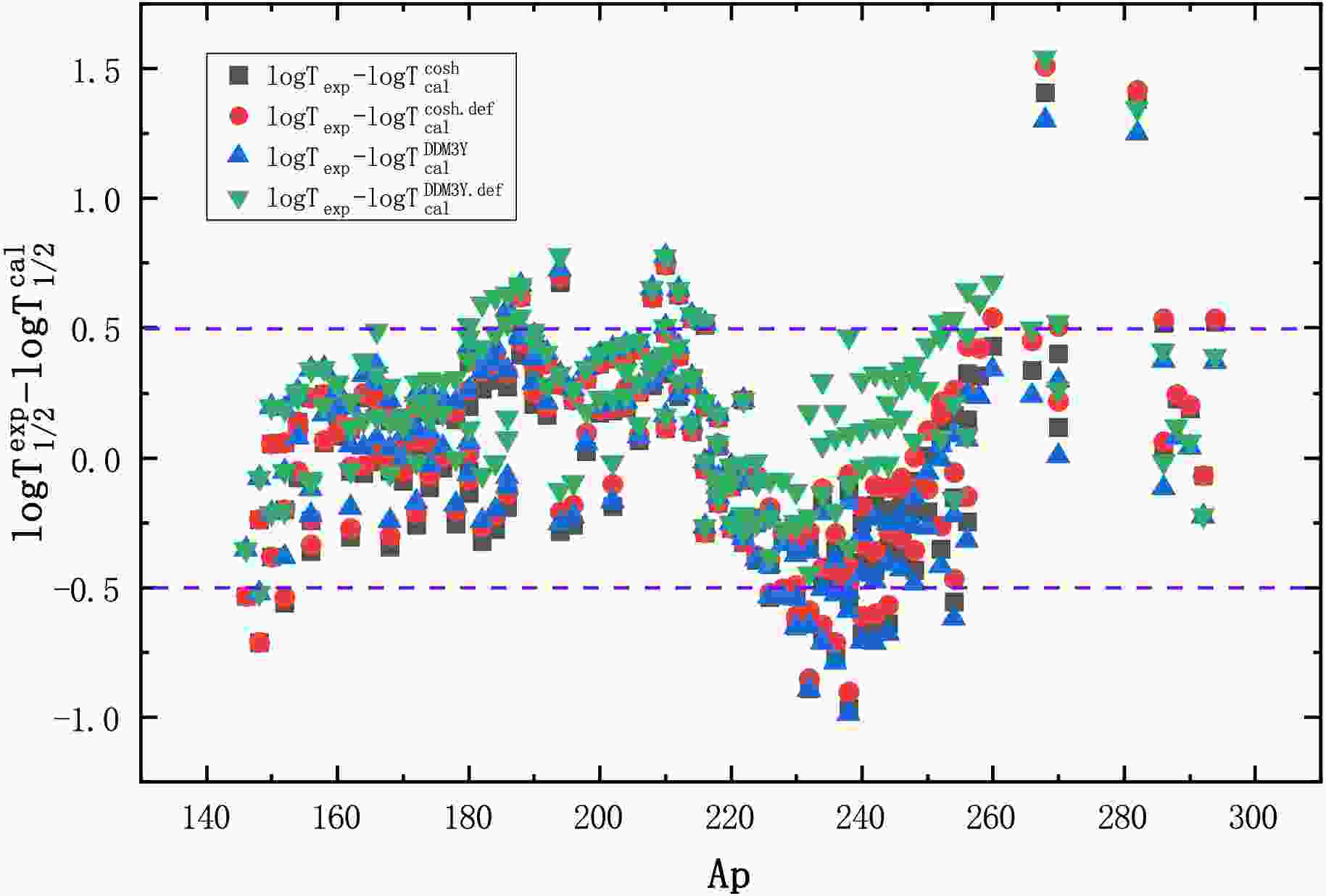
$Q_{\alpha}$ , the preformation factors$P_{\alpha}$ calculated using the CFM, and the quadrupole ($\beta_2$ ) and hexadecapole ($\beta_4$ ) deformation parameters taken from the FRDM mass table. The next five columns show the experimental half-lives$T^{\mathrm{exp}}_{1/2}$ and the calculated half-lives obtained using the cosh potential and the microscopic DDM3Y double-folding potential under both spherical and deformation-averaged calculations, respectively. For a more intuitive comparison, the experimental data and calculated results are plotted on a logarithmic scale in Fig. 1. As shown in this figure, the four calculations exhibit a similar overall dependence on the parent mass number, and most logarithmic deviations remain within the interval from$ -0.5 $ to$ 0.5 $ . However, two conspicuous outliers appear at$ ^{268}\text{Hs} $ ($ Z = 108 $ ,$ N = 160 $ ) and$ ^{282}\text{Ds} $ ($ Z = 110 $ ,$ N = 172 $ ), where the deviations exceed one order of magnitude.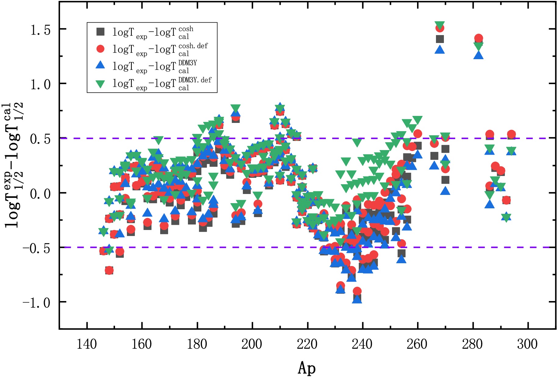
Figure 1. (color online) Logarithmic of deviations between the calculated half-lives and experimental data as a function of mass numbers. The results obtained with the spherical and deformed cosh and DDM3Y potentials are shown by different symbols.
α transition $Q_{\alpha}$ $P_{\alpha}$ $\beta_2$ $\beta_4$ $T_{1/2}^{\text{exp}}$ $T_{1/2}^{\text{Cosh}}$ $T_{1/2}^{\text{Cosh, Def.}}$ $T_{1/2}^{\text{DDM3Y}}$ $T_{1/2}^{\text{DDM3Y, Def.}}$ $^{146}\text{Sm}\to^{142}\text{Nd}$ 2.529 0.198 0.000 0.000 $2.15\times10^{15}$ $7.37\times10^{15}$ $7.37\times10^{15}$ $4.85\times10^{15}$ $4.85\times10^{15}$ $^{148}\text{Sm}\to^{144}\text{Nd}$ 1.987 0.195 0.000 0.000 $1.99\times10^{23}$ $1.03\times10^{24}$ $1.03\times10^{24}$ $6.64\times10^{23}$ $6.64\times10^{23}$ $^{148}\text{Gd}\to^{144}\text{Sm}$ 3.271 0.202 0.000 0.000 $2.25\times10^{9}$ $3.90\times10^{9}$ $3.90\times10^{9}$ $2.68\times10^{9}$ $2.68\times10^{9}$ $^{150}\text{Gd}\to^{146}\text{Sm}$ 2.807 0.202 0.000 0.000 $5.65\times10^{13}$ $1.36\times10^{14}$ $1.36\times10^{14}$ $9.27\times10^{13}$ $9.27\times10^{13}$ $^{152}\text{Gd}\to^{148}\text{Sm}$ 2.204 0.221 0.172 0.060 $3.41\times10^{21}$ $1.24\times10^{22}$ $1.18\times10^{22}$ $8.26\times10^{21}$ $5.48\times10^{21}$ $^{150}\text{Dy}\to^{146}\text{Gd}$ 4.351 0.236 0.000 0.000 $1.28\times10^{3}$ $1.13\times10^{3}$ $1.13\times10^{3}$ $8.12\times10^{2}$ $8.12\times10^{2}$ $^{152}\text{Dy}\to^{148}\text{Gd}$ 3.726 0.240 0.000 0.000 $8.51\times10^{6}$ $1.35\times10^{7}$ $1.35\times10^{7}$ $9.62\times10^{6}$ $9.62\times10^{6}$ $^{154}\text{Dy}\to^{150}\text{Gd}$ 2.945 0.238 0.172 0.047 $9.47\times10^{13}$ $1.13\times10^{14}$ $1.07\times10^{14}$ $7.87\times10^{13}$ $5.52\times10^{13}$ $^{152}\text{Er}\to^{148}\text{Dy}$ 4.934 0.239 0.011 0.000 $1.14\times10^{1}$ $1.00\times10^{1}$ $1.00\times10^{1}$ $7.42\times10^{0}$ $7.41\times10^{0}$ $^{154}\text{Er}\to^{150}\text{Dy}$ 4.280 0.257 0.000 0.000 $4.75\times10^{4}$ $3.71\times10^{4}$ $3.71\times10^{4}$ $2.72\times10^{4}$ $2.72\times10^{4}$ $^{156}\text{Er}\to^{152}\text{Dy}$ 3.481 0.252 0.172 0.035 $9.75\times10^{9}$ $2.25\times10^{10}$ $2.12\times10^{10}$ $1.62\times10^{10}$ $1.18\times10^{10}$ $^{154}\text{Yb}\to^{150}\text{Er}$ 5.474 0.235 0.011 0.000 $4.42\times10^{-1}$ $3.23\times10^{-1}$ $3.23\times10^{-1}$ $2.45\times10^{-1}$ $2.45\times10^{-1}$ $^{156}\text{Yb}\to^{152}\text{Er}$ 4.809 0.257 −0.084 0.014 $2.56\times10^{2}$ $4.46\times10^{2}$ $4.38\times10^{2}$ $3.36\times10^{2}$ $3.21\times10^{2}$ $^{156}\text{Hf}\to^{152}\text{Yb}$ 6.025 0.270 0.000 0.000 $2.30\times10^{-2}$ $1.35\times10^{-2}$ $1.35\times10^{-2}$ $1.05\times10^{-2}$ $1.05\times10^{-2}$ $^{158}\text{Hf}\to^{154}\text{Yb}$ 5.405 0.246 −0.104 0.028 $6.43\times10^{0}$ $5.66\times10^{0}$ $5.51\times10^{0}$ $4.38\times10^{0}$ $4.05\times10^{0}$ $^{160}\text{Hf}\to^{156}\text{Yb}$ 4.902 0.255 0.139 0.044 $1.89\times10^{3}$ $1.57\times10^{3}$ $1.50\times10^{3}$ $1.21\times10^{3}$ $9.71\times10^{2}$ $^{162}\text{Hf}\to^{158}\text{Yb}$ 4.417 0.241 0.183 0.025 $4.86\times10^{5}$ $9.82\times10^{5}$ $9.14\times10^{5}$ $7.55\times10^{5}$ $5.42\times10^{5}$ $^{158}\text{W}\to^{154}\text{Hf}$ 6.615 0.241 0.021 0.000 $1.43\times10^{-3}$ $8.14\times10^{-4}$ $8.13\times10^{-4}$ $6.46\times10^{-4}$ $6.45\times10^{-4}$ $^{160}\text{W}\to^{156}\text{Hf}$ 6.065 0.273 −0.084 0.014 $1.03\times10^{-1}$ $7.09\times10^{-2}$ $6.96\times10^{-2}$ $5.63\times10^{-2}$ $5.38\times10^{-2}$ $^{162}\text{W}\to^{158}\text{Hf}$ 5.678 0.244 0.128 0.030 $2.63\times10^{0}$ $2.96\times10^{0}$ $2.85\times10^{0}$ $2.35\times10^{0}$ $2.01\times10^{0}$ $^{164}\text{W}\to^{160}\text{Hf}$ 5.278 0.251 0.161 0.022 $1.65\times10^{2}$ $1.89\times10^{2}$ $1.78\times10^{2}$ $1.50\times10^{2}$ $1.18\times10^{2}$ $^{166}\text{W}\to^{162}\text{Hf}$ 4.856 0.231 0.183 0.013 $5.47\times10^{4}$ $3.05\times10^{4}$ $2.83\times10^{4}$ $2.41\times10^{4}$ $1.78\times10^{4}$ $^{168}\text{W}\to^{164}\text{Hf}$ 4.500 0.236 0.206 0.016 $1.59\times10^{6}$ $3.52\times10^{6}$ $3.20\times10^{6}$ $2.77\times10^{6}$ $1.83\times10^{6}$ $^{180}\text{W}\to^{176}\text{Hf}$ 2.515 0.162 0.278 −0.057 $5.02\times10^{25}$ $5.67\times10^{25}$ $4.84\times10^{25}$ $4.34\times10^{25}$ $2.11\times10^{25}$ $^{162}\text{Os}\to^{158}\text{W}$ 6.765 0.237 0.085 0.003 $2.10\times10^{-3}$ $1.64\times10^{-3}$ $1.61\times10^{-3}$ $1.33\times10^{-3}$ $1.27\times10^{-3}$ $^{164}\text{Os}\to^{160}\text{W}$ 6.485 0.271 0.128 0.018 $2.18\times10^{-2}$ $1.29\times10^{-2}$ $1.23\times10^{-2}$ $1.05\times10^{-2}$ $9.16\times10^{-3}$ $^{166}\text{Os}\to^{162}\text{W}$ 6.142 0.247 0.150 0.020 $2.55\times10^{-1}$ $2.63\times10^{-1}$ $2.49\times10^{-1}$ $2.14\times10^{-1}$ $1.76\times10^{-1}$ $^{168}\text{Os}\to^{164}\text{W}$ 5.816 0.247 0.173 −0.001 $4.84\times10^{0}$ $5.46\times10^{0}$ $5.07\times10^{0}$ $4.44\times10^{0}$ $3.51\times10^{0}$ $^{170}\text{Os}\to^{166}\text{W}$ 5.536 0.237 0.184 0.001 $7.75\times10^{1}$ $9.52\times10^{1}$ $8.77\times10^{1}$ $7.74\times10^{1}$ $5.84\times10^{1}$ $^{172}\text{Os}\to^{168}\text{W}$ 5.224 0.240 0.206 −0.009 $1.61\times10^{3}$ $2.92\times10^{3}$ $2.64\times10^{3}$ $2.38\times10^{3}$ $1.67\times10^{3}$ $^{174}\text{Os}\to^{170}\text{W}$ 4.871 0.226 0.217 −0.007 $1.78\times10^{5}$ $2.32\times10^{5}$ $2.08\times10^{5}$ $1.89\times10^{5}$ $1.25\times10^{5}$ $^{186}\text{Os}\to^{182}\text{W}$ 2.821 0.157 0.232 −0.066 $6.31\times10^{22}$ $9.44\times10^{22}$ $8.37\times10^{22}$ $7.50\times10^{22}$ $4.44\times10^{22}$ $^{166}\text{Pt}\to^{162}\text{Os}$ 7.295 0.238 0.107 −0.008 $2.94\times10^{-4}$ $1.81\times10^{-4}$ $1.75\times10^{-4}$ $1.50\times10^{-4}$ $1.39\times10^{-4}$ $^{168}\text{Pt}\to^{164}\text{Os}$ 6.985 0.272 0.129 0.006 $2.02\times10^{-3}$ $1.45\times10^{-3}$ $1.39\times10^{-3}$ $1.21\times10^{-3}$ $1.07\times10^{-3}$ $^{170}\text{Pt}\to^{166}\text{Os}$ 6.708 0.242 0.151 −0.004 $1.39\times10^{-2}$ $1.35\times10^{-2}$ $1.28\times10^{-2}$ $1.13\times10^{-2}$ $9.56\times10^{-3}$ $^{172}\text{Pt}\to^{168}\text{Os}$ 6.463 0.254 0.173 −0.013 $1.01\times10^{-1}$ $9.33\times10^{-2}$ $8.63\times10^{-2}$ $7.79\times10^{-2}$ $6.25\times10^{-2}$ $^{174}\text{Pt}\to^{170}\text{Os}$ 6.183 0.247 0.184 −0.012 $1.15\times10^{0}$ $1.09\times10^{0}$ $1.00\times10^{0}$ $9.15\times10^{-1}$ $6.98\times10^{-1}$ $^{176}\text{Pt}\to^{172}\text{Os}$ 5.885 0.261 0.195 −0.010 $1.57\times10^{1}$ $1.72\times10^{1}$ $1.56\times10^{1}$ $1.44\times10^{1}$ $1.06\times10^{1}$ $^{178}\text{Pt}\to^{174}\text{Os}$ 5.573 0.227 0.217 −0.007 $2.68\times10^{2}$ $4.83\times10^{2}$ $4.30\times10^{2}$ $4.04\times10^{2}$ $2.69\times10^{2}$ $^{180}\text{Pt}\to^{176}\text{Os}$ 5.276 0.205 0.218 −0.019 $1.07\times10^{4}$ $1.47\times10^{4}$ $1.31\times10^{4}$ $1.23\times10^{4}$ $8.22\times10^{3}$ $^{182}\text{Pt}\to^{178}\text{Os}$ 4.951 0.187 0.219 −0.031 $4.19\times10^{5}$ $8.79\times10^{5}$ $7.81\times10^{5}$ $7.36\times10^{5}$ $4.89\times10^{5}$ $^{184}\text{Pt}\to^{180}\text{Os}$ 4.599 0.186 0.219 −0.043 $5.86\times10^{7}$ $1.11\times10^{8}$ $9.87\times10^{7}$ $9.29\times10^{7}$ $6.13\times10^{7}$ $^{186}\text{Pt}\to^{182}\text{Os}$ 4.320 0.173 0.220 −0.056 $5.35\times10^{9}$ $8.29\times10^{9}$ $7.36\times10^{9}$ $6.92\times10^{9}$ $4.51\times10^{9}$ $^{188}\text{Pt}\to^{184}\text{Os}$ 4.007 0.216 0.220 −0.068 $3.38\times10^{12}$ $1.36\times10^{12}$ $1.21\times10^{12}$ $1.14\times10^{12}$ $7.26\times10^{11}$ $^{190}\text{Pt}\to^{186}\text{Os}$ 3.269 0.203 0.209 −0.083 $1.52\times10^{19}$ $9.46\times10^{18}$ $8.50\times10^{18}$ $7.80\times10^{18}$ $4.95\times10^{18}$ $^{172}\text{Hg}\to^{168}\text{Pt}$ 7.525 0.277 0.118 0.005 $2.31\times10^{-4}$ $1.55\times10^{-4}$ $1.49\times10^{-4}$ $1.31\times10^{-4}$ $1.19\times10^{-4}$ $^{174}\text{Hg}\to^{170}\text{Pt}$ 7.233 0.249 0.129 −0.006 $2.00\times10^{-3}$ $1.31\times10^{-3}$ $1.25\times10^{-3}$ $1.12\times10^{-3}$ $9.94\times10^{-4}$ $^{176}\text{Hg}\to^{172}\text{Pt}$ 6.897 0.267 0.140 −0.005 $2.23\times10^{-2}$ $1.53\times10^{-2}$ $1.45\times10^{-2}$ $1.31\times10^{-2}$ $1.13\times10^{-2}$ $^{178}\text{Hg}\to^{174}\text{Pt}$ 6.577 0.258 0.162 −0.003 $2.98\times10^{-1}$ $2.12\times10^{-1}$ $1.98\times10^{-1}$ $1.82\times10^{-1}$ $1.47\times10^{-1}$ $^{180}\text{Hg}\to^{176}\text{Pt}$ 6.258 0.265 0.239 0.021 $5.37\times10^{0}$ $3.42\times10^{0}$ $2.96\times10^{0}$ $2.93\times10^{0}$ $1.66\times10^{0}$ $^{182}\text{Hg}\to^{178}\text{Pt}$ 5.995 0.254 0.250 0.011 $7.80\times10^{1}$ $4.23\times10^{1}$ $3.61\times10^{1}$ $3.63\times10^{1}$ $1.99\times10^{1}$ $^{184}\text{Hg}\to^{180}\text{Pt}$ 5.660 0.242 0.251 −0.002 $2.77\times10^{3}$ $1.39\times10^{3}$ $1.19\times10^{3}$ $1.20\times10^{3}$ $6.63\times10^{2}$ $^{186}\text{Hg}\to^{182}\text{Pt}$ 5.204 0.247 0.219 −0.031 $5.02\times10^{5}$ $2.68\times10^{5}$ $2.37\times10^{5}$ $2.31\times10^{5}$ $1.52\times10^{5}$ $^{188}\text{Hg}\to^{184}\text{Pt}$ 4.709 0.239 0.219 −0.044 $5.27\times10^{8}$ $2.12\times10^{8}$ $1.87\times10^{8}$ $1.82\times10^{8}$ $1.18\times10^{8}$ $^{180}\text{Pb}\to^{176}\text{Hg}$ 7.419 0.248 −0.115 −0.030 $4.10\times10^{-3}$ $1.74\times10^{-3}$ $1.66\times10^{-3}$ $1.52\times10^{-3}$ $1.41\times10^{-3}$ $^{182}\text{Pb}\to^{178}\text{Hg}$ 7.065 0.234 −0.125 −0.017 $5.50\times10^{-2}$ $2.57\times10^{-2}$ $2.44\times10^{-2}$ $2.26\times10^{-2}$ $2.06\times10^{-2}$ $^{184}\text{Pb}\to^{180}\text{Hg}$ 6.774 0.236 −0.135 −0.005 $6.12\times10^{-1}$ $2.59\times10^{-1}$ $2.44\times10^{-1}$ $2.28\times10^{-1}$ $2.03\times10^{-1}$ $^{186}\text{Pb}\to^{182}\text{Hg}$ 6.471 0.230 −0.146 −0.004 $1.18\times10^{1}$ $3.56\times10^{0}$ $3.32\times10^{0}$ $3.14\times10^{0}$ $2.74\times10^{0}$ $^{188}\text{Pb}\to^{184}\text{Hg}$ 6.109 0.221 −0.146 −0.004 $2.94\times10^{2}$ $1.10\times10^{2}$ $1.02\times10^{2}$ $9.71\times10^{1}$ $8.42\times10^{1}$ $^{190}\text{Pb}\to^{186}\text{Hg}$ 5.697 0.216 −0.146 −0.004 $1.76\times10^{4}$ $8.24\times10^{3}$ $7.69\times10^{3}$ $7.29\times10^{3}$ $6.28\times10^{3}$ $^{192}\text{Pb}\to^{188}\text{Hg}$ 5.221 0.204 −0.146 −0.015 $3.52\times10^{6}$ $2.42\times10^{6}$ $2.26\times10^{6}$ $2.14\times10^{6}$ $1.84\times10^{6}$ $^{194}\text{Pb}\to^{190}\text{Hg}$ 4.738 0.195 −0.125 −0.017 $8.79\times10^{9}$ $1.86\times10^{9}$ $1.77\times10^{9}$ $1.65\times10^{9}$ $1.46\times10^{9}$ $^{210}\text{Pb}\to^{206}\text{Hg}$ 3.793 0.107 0.000 0.000 $3.69\times10^{16}$ $2.85\times10^{16}$ $2.85\times10^{16}$ $2.54\times10^{16}$ $2.54\times10^{16}$ $^{188}\text{Po}\to^{184}\text{Pb}$ 8.083 0.275 0.000 0.012 $2.70\times10^{-4}$ $6.48\times10^{-5}$ $6.48\times10^{-5}$ $5.80\times10^{-5}$ $5.79\times10^{-5}$ $^{190}\text{Po}\to^{186}\text{Pb}$ 7.693 0.262 0.000 0.000 $2.45\times10^{-3}$ $9.22\times10^{-4}$ $9.22\times10^{-4}$ $8.30\times10^{-4}$ $8.30\times10^{-4}$ $^{192}\text{Po}\to^{188}\text{Pb}$ 7.320 0.257 0.000 0.000 $3.22\times10^{-2}$ $1.40\times10^{-2}$ $1.40\times10^{-2}$ $1.26\times10^{-2}$ $1.26\times10^{-2}$ $^{194}\text{Po}\to^{190}\text{Pb}$ 6.987 0.235 0.000 0.000 $3.92\times10^{-1}$ $2.05\times10^{-1}$ $2.05\times10^{-1}$ $1.86\times10^{-1}$ $1.86\times10^{-1}$ $^{196}\text{Po}\to^{192}\text{Pb}$ 6.658 0.216 0.000 0.000 $5.96\times10^{0}$ $3.56\times10^{0}$ $3.56\times10^{0}$ $3.24\times10^{0}$ $3.24\times10^{0}$ $^{198}\text{Po}\to^{194}\text{Pb}$ 6.310 0.203 0.000 0.000 $1.85\times10^{2}$ $9.17\times10^{1}$ $9.17\times10^{1}$ $8.36\times10^{1}$ $8.36\times10^{1}$ $^{200}\text{Po}\to^{196}\text{Pb}$ 5.981 0.184 0.000 0.000 $6.20\times10^{3}$ $2.69\times10^{3}$ $2.69\times10^{3}$ $2.46\times10^{3}$ $2.46\times10^{3}$ $^{202}\text{Po}\to^{198}\text{Pb}$ 5.700 0.177 0.000 0.000 $1.39\times10^{5}$ $5.75\times10^{4}$ $5.75\times10^{4}$ $5.26\times10^{4}$ $5.26\times10^{4}$ $^{204}\text{Po}\to^{200}\text{Pb}$ 5.485 0.158 0.000 0.000 $1.88\times10^{6}$ $7.49\times10^{5}$ $7.49\times10^{5}$ $6.87\times10^{5}$ $6.87\times10^{5}$ $^{206}\text{Po}\to^{202}\text{Pb}$ 5.327 0.145 0.000 0.000 $1.39\times10^{7}$ $5.33\times10^{6}$ $5.33\times10^{6}$ $4.90\times10^{6}$ $4.90\times10^{6}$ $^{208}\text{Po}\to^{204}\text{Pb}$ 5.216 0.135 0.000 0.000 $9.15\times10^{7}$ $2.21\times10^{7}$ $2.21\times10^{7}$ $2.04\times10^{7}$ $2.04\times10^{7}$ $^{210}\text{Po}\to^{206}\text{Pb}$ 5.407 0.106 0.000 0.000 $1.20\times10^{7}$ $2.17\times10^{6}$ $2.17\times10^{6}$ $2.00\times10^{6}$ $2.00\times10^{6}$ $^{212}\text{Po}\to^{208}\text{Pb}$ 8.954 0.221 0.000 0.000 $2.94\times10^{-7}$ $1.19\times10^{-7}$ $1.19\times10^{-7}$ $1.09\times10^{-7}$ $1.09\times10^{-7}$ $^{214}\text{Po}\to^{210}\text{Pb}$ 7.833 0.213 0.000 0.000 $1.63\times10^{-4}$ $1.30\times10^{-4}$ $1.30\times10^{-4}$ $1.20\times10^{-4}$ $1.20\times10^{-4}$ $^{216}\text{Po}\to^{212}\text{Pb}$ 6.906 0.205 0.000 0.000 $1.44\times10^{-1}$ $1.60\times10^{-1}$ $1.60\times10^{-1}$ $1.49\times10^{-1}$ $1.49\times10^{-1}$ $^{218}\text{Po}\to^{214}\text{Pb}$ 6.115 0.196 0.000 0.000 $1.86\times10^{2}$ $2.58\times10^{2}$ $2.58\times10^{2}$ $2.41\times10^{2}$ $2.41\times10^{2}$ $^{194}\text{Rn}\to^{190}\text{Po}$ 7.863 0.261 −0.217 0.017 $7.80\times10^{-4}$ $1.51\times10^{-3}$ $1.27\times10^{-3}$ $1.39\times10^{-3}$ $1.04\times10^{-3}$ $^{196}\text{Rn}\to^{192}\text{Po}$ 7.616 0.256 −0.217 0.017 $4.70\times10^{-3}$ $8.53\times10^{-3}$ $7.16\times10^{-3}$ $7.89\times10^{-3}$ $5.83\times10^{-3}$ $^{198}\text{Rn}\to^{194}\text{Po}$ 7.350 0.239 −0.207 0.015 $6.87\times10^{-2}$ $6.48\times10^{-2}$ $5.53\times10^{-2}$ $6.02\times10^{-2}$ $4.53\times10^{-2}$ $^{200}\text{Rn}\to^{196}\text{Po}$ 7.044 0.221 0.085 0.003 $1.17\times10^{0}$ $7.86\times10^{-1}$ $7.68\times10^{-1}$ $7.32\times10^{-1}$ $6.86\times10^{-1}$ $^{202}\text{Rn}\to^{198}\text{Po}$ 6.773 0.209 0.075 0.002 $1.23\times10^{1}$ $8.10\times10^{0}$ $7.95\times10^{0}$ $7.57\times10^{0}$ $7.19\times10^{0}$ $^{204}\text{Rn}\to^{200}\text{Po}$ 6.547 0.191 −0.063 0.013 $1.03\times10^{2}$ $6.55\times10^{1}$ $6.46\times10^{1}$ $6.14\times10^{1}$ $6.05\times10^{1}$ $^{206}\text{Rn}\to^{202}\text{Po}$ 6.384 0.180 −0.063 0.001 $5.46\times10^{2}$ $3.07\times10^{2}$ $3.03\times10^{2}$ $2.89\times10^{2}$ $2.79\times10^{2}$ $^{208}\text{Rn}\to^{204}\text{Po}$ 6.261 0.163 −0.042 0.001 $2.33\times10^{3}$ $1.06\times10^{3}$ $1.06\times10^{3}$ $1.00\times10^{3}$ $9.88\times10^{2}$ $^{210}\text{Rn}\to^{206}\text{Po}$ 6.159 0.152 0.000 0.000 $8.99\times10^{3}$ $2.97\times10^{3}$ $2.97\times10^{3}$ $2.81\times10^{3}$ $2.81\times10^{3}$ $^{212}\text{Rn}\to^{208}\text{Po}$ 6.385 0.121 0.000 0.000 $1.43\times10^{3}$ $3.38\times10^{2}$ $3.38\times10^{2}$ $3.20\times10^{2}$ $3.20\times10^{2}$ $^{214}\text{Rn}\to^{210}\text{Po}$ 9.208 0.229 0.000 0.000 $2.59\times10^{-7}$ $1.36\times10^{-7}$ $1.36\times10^{-7}$ $1.27\times10^{-7}$ $1.27\times10^{-7}$ $^{216}\text{Rn}\to^{212}\text{Po}$ 8.197 0.237 0.000 0.000 $2.90\times10^{-5}$ $5.64\times10^{-5}$ $5.64\times10^{-5}$ $5.32\times10^{-5}$ $5.32\times10^{-5}$ $^{218}\text{Rn}\to^{214}\text{Po}$ 7.262 0.234 0.000 0.000 $3.38\times10^{-2}$ $5.04\times10^{-2}$ $5.04\times10^{-2}$ $4.79\times10^{-2}$ $4.79\times10^{-2}$ $^{220}\text{Rn}\to^{216}\text{Po}$ 6.405 0.221 0.000 0.000 $5.56\times10^{1}$ $1.04\times10^{2}$ $1.04\times10^{2}$ $9.91\times10^{1}$ $9.91\times10^{1}$ $^{222}\text{Rn}\to^{218}\text{Po}$ 5.590 0.222 0.056 0.028 $3.30\times10^{5}$ $7.04\times10^{5}$ $6.97\times10^{5}$ $6.75\times10^{5}$ $6.38\times10^{5}$ $^{202}\text{Ra}\to^{198}\text{Rn}$ 7.880 0.248 −0.227 0.019 $4.10\times10^{-3}$ $6.33\times10^{-3}$ $5.19\times10^{-3}$ $6.02\times10^{-3}$ $4.29\times10^{-3}$ $^{204}\text{Ra}\to^{200}\text{Rn}$ 7.636 0.231 −0.207 0.004 $6.00\times10^{-2}$ $3.83\times10^{-2}$ $3.24\times10^{-2}$ $3.65\times10^{-2}$ $2.77\times10^{-2}$ $^{206}\text{Ra}\to^{202}\text{Rn}$ 7.416 0.219 −0.115 0.017 $2.40\times10^{-1}$ $2.07\times10^{-1}$ $1.97\times10^{-1}$ $1.98\times10^{-1}$ $1.78\times10^{-1}$ $^{208}\text{Ra}\to^{204}\text{Rn}$ 7.273 0.195 −0.115 0.017 $1.27\times10^{0}$ $6.73\times10^{-1}$ $6.41\times10^{-1}$ $6.46\times10^{-1}$ $5.79\times10^{-1}$ $^{210}\text{Ra}\to^{206}\text{Rn}$ 7.151 0.187 −0.094 0.015 $4.00\times10^{0}$ $1.78\times10^{0}$ $1.72\times10^{0}$ $1.71\times10^{0}$ $1.59\times10^{0}$ $^{214}\text{Ra}\to^{210}\text{Rn}$ 7.273 0.138 0.000 0.000 $2.44\times10^{0}$ $7.08\times10^{-1}$ $7.08\times10^{-1}$ $6.85\times10^{-1}$ $6.85\times10^{-1}$ $^{216}\text{Ra}\to^{212}\text{Rn}$ 9.525 0.239 0.000 0.000 $1.72\times10^{-7}$ $1.09\times10^{-7}$ $1.09\times10^{-7}$ $1.04\times10^{-7}$ $1.04\times10^{-7}$ $^{218}\text{Ra}\to^{214}\text{Rn}$ 8.541 0.243 0.000 0.000 $2.59\times10^{-5}$ $3.21\times10^{-5}$ $3.21\times10^{-5}$ $3.09\times10^{-5}$ $3.09\times10^{-5}$ $^{220}\text{Ra}\to^{216}\text{Rn}$ 7.594 0.239 0.000 0.000 $1.81\times10^{-2}$ $2.35\times10^{-2}$ $2.35\times10^{-2}$ $2.28\times10^{-2}$ $2.28\times10^{-2}$ $^{222}\text{Ra}\to^{218}\text{Rn}$ 6.678 0.199 0.079 0.054 $3.36\times10^{1}$ $6.56\times10^{1}$ $6.42\times10^{1}$ $6.42\times10^{1}$ $5.52\times10^{1}$ $^{224}\text{Ra}\to^{220}\text{Rn}$ 5.789 0.184 0.110 0.068 $3.14\times10^{5}$ $7.84\times10^{5}$ $7.54\times10^{5}$ $7.71\times10^{5}$ $5.59\times10^{5}$ $^{226}\text{Ra}\to^{222}\text{Rn}$ 4.871 0.182 0.110 0.068 $5.05\times10^{10}$ $1.75\times10^{11}$ $1.69\times10^{11}$ $1.73\times10^{11}$ $1.22\times10^{11}$ $^{210}\text{Th}\to^{206}\text{Ra}$ 8.069 0.234 −0.125 0.018 $1.60\times10^{-2}$ $7.59\times10^{-3}$ $7.14\times10^{-3}$ $7.43\times10^{-3}$ $6.57\times10^{-3}$ $^{212}\text{Th}\to^{208}\text{Ra}$ 7.958 0.196 −0.125 0.018 $3.17\times10^{-2}$ $1.85\times10^{-2}$ $1.74\times10^{-2}$ $1.82\times10^{-2}$ $1.60\times10^{-2}$ $^{214}\text{Th}\to^{210}\text{Ra}$ 7.827 0.195 −0.084 −0.009 $8.70\times10^{-2}$ $4.48\times10^{-2}$ $4.36\times10^{-2}$ $4.41\times10^{-2}$ $4.19\times10^{-2}$ $^{216}\text{Th}\to^{212}\text{Ra}$ 8.073 0.159 −0.053 −0.011 $2.63\times10^{-2}$ $8.13\times10^{-3}$ $8.04\times10^{-3}$ $8.00\times10^{-3}$ $7.83\times10^{-3}$ $^{218}\text{Th}\to^{214}\text{Ra}$ 9.849 0.251 0.000 0.000 $1.22\times10^{-7}$ $8.54\times10^{-8}$ $8.54\times10^{-8}$ $8.27\times10^{-8}$ $8.27\times10^{-8}$ $^{220}\text{Th}\to^{216}\text{Ra}$ 8.974 0.243 0.000 0.000 $1.02\times10^{-5}$ $1.12\times10^{-5}$ $1.12\times10^{-5}$ $1.10\times10^{-5}$ $1.10\times10^{-5}$ $^{222}\text{Th}\to^{218}\text{Ra}$ 8.132 0.232 0.078 0.054 $2.24\times10^{-3}$ $2.73\times10^{-3}$ $2.67\times10^{-3}$ $2.71\times10^{-3}$ $2.36\times10^{-3}$ $^{224}\text{Th}\to^{220}\text{Ra}$ 7.299 0.198 0.111 0.081 $1.04\times10^{0}$ $1.86\times10^{0}$ $1.78\times10^{0}$ $1.86\times10^{0}$ $1.30\times10^{0}$ $^{226}\text{Th}\to^{222}\text{Ra}$ 6.453 0.182 0.122 0.082 $1.84\times10^{3}$ $4.77\times10^{3}$ $4.54\times10^{3}$ $4.81\times10^{3}$ $3.10\times10^{3}$ $^{228}\text{Th}\to^{224}\text{Ra}$ 5.520 0.183 0.143 0.084 $6.04\times10^{7}$ $2.06\times10^{8}$ $1.93\times10^{8}$ $2.08\times10^{8}$ $1.14\times10^{8}$ $^{230}\text{Th}\to^{226}\text{Ra}$ 4.770 0.183 0.164 0.098 $2.38\times10^{12}$ $1.06\times10^{13}$ $9.75\times10^{12}$ $1.07\times10^{13}$ $4.38\times10^{12}$ $^{232}\text{Th}\to^{228}\text{Ra}$ 4.082 0.160 0.174 0.099 $4.42\times10^{17}$ $3.42\times10^{18}$ $3.13\times10^{18}$ $3.47\times10^{18}$ $1.23\times10^{18}$ $^{218}\text{U}\to^{214}\text{Th}$ 8.775 0.188 −0.063 −0.022 $3.54\times10^{-4}$ $3.19\times10^{-4}$ $3.14\times10^{-4}$ $3.20\times10^{-4}$ $3.10\times10^{-4}$ $^{222}\text{U}\to^{218}\text{Th}$ 9.478 0.245 0.000 0.000 $4.70\times10^{-6}$ $2.83\times10^{-6}$ $2.83\times10^{-6}$ $2.82\times10^{-6}$ $2.82\times10^{-6}$ $^{224}\text{U}\to^{220}\text{Th}$ 8.628 0.247 0.090 0.055 $3.96\times10^{-4}$ $4.79\times10^{-4}$ $4.65\times10^{-4}$ $4.84\times10^{-4}$ $4.09\times10^{-4}$ $^{226}\text{U}\to^{222}\text{Th}$ 7.701 0.208 0.111 0.069 $2.69\times10^{-1}$ $4.36\times10^{-1}$ $4.17\times10^{-1}$ $4.46\times10^{-1}$ $3.30\times10^{-1}$ $^{228}\text{U}\to^{224}\text{Th}$ 6.799 0.190 0.144 0.084 $5.60\times10^{2}$ $1.17\times10^{3}$ $1.09\times10^{3}$ $1.21\times10^{3}$ $6.84\times10^{2}$ $^{230}\text{U}\to^{226}\text{Th}$ 5.992 0.187 0.154 0.085 $1.75\times10^{6}$ $5.86\times10^{6}$ $5.43\times10^{6}$ $6.09\times10^{6}$ $3.10\times10^{6}$ $^{232}\text{U}\to^{228}\text{Th}$ 5.414 0.169 0.174 0.100 $2.17\times10^{9}$ $9.24\times10^{9}$ $8.41\times10^{9}$ $9.64\times10^{9}$ $3.64\times10^{9}$ $^{234}\text{U}\to^{230}\text{Th}$ 4.858 0.150 0.195 0.114 $7.75\times10^{12}$ $3.83\times10^{13}$ $3.42\times10^{13}$ $4.00\times10^{13}$ $1.06\times10^{13}$ $^{236}\text{U}\to^{232}\text{Th}$ 4.573 0.153 0.205 0.103 $7.39\times10^{14}$ $4.32\times10^{15}$ $3.82\times10^{15}$ $4.53\times10^{15}$ $1.19\times10^{15}$ $^{238}\text{U}\to^{234}\text{Th}$ 4.270 0.137 0.226 0.095 $1.41\times10^{17}$ $1.30\times10^{18}$ $1.12\times10^{18}$ $1.36\times10^{18}$ $3.10\times10^{17}$ $^{230}\text{Pu}\to^{226}\text{U}$ 7.178 0.201 0.143 0.084 $1.05\times10^{2}$ $2.35\times10^{2}$ $2.19\times10^{2}$ $2.49\times10^{2}$ $1.41\times10^{2}$ $^{232}\text{Pu}\to^{228}\text{U}$ 6.716 0.165 0.186 0.126 $1.01\times10^{4}$ $2.18\times10^{4}$ $1.94\times10^{4}$ $2.31\times10^{4}$ $6.74\times10^{3}$ $^{234}\text{Pu}\to^{230}\text{U}$ 6.310 0.152 0.185 0.126 $5.28\times10^{5}$ $1.57\times10^{6}$ $1.41\times10^{6}$ $1.68\times10^{6}$ $4.74\times10^{5}$ $^{236}\text{Pu}\to^{232}\text{U}$ 5.867 0.140 0.206 0.116 $9.02\times10^{7}$ $2.82\times10^{8}$ $2.47\times10^{8}$ $3.03\times10^{8}$ $7.56\times10^{7}$ $^{238}\text{Pu}\to^{234}\text{U}$ 5.593 0.145 0.215 0.106 $2.77\times10^{9}$ $8.46\times10^{9}$ $7.33\times10^{9}$ $9.12\times10^{9}$ $2.25\times10^{9}$ $^{240}\text{Pu}\to^{236}\text{U}$ 5.256 0.129 0.226 0.108 $2.07\times10^{11}$ $9.83\times10^{11}$ $8.41\times10^{11}$ $1.06\times10^{12}$ $2.24\times10^{11}$ $^{242}\text{Pu}\to^{238}\text{U}$ 4.984 0.133 0.236 0.098 $1.18\times10^{13}$ $5.60\times10^{13}$ $4.74\times10^{13}$ $6.07\times10^{13}$ $1.25\times10^{13}$ $^{244}\text{Pu}\to^{240}\text{U}$ 4.666 0.127 0.237 0.086 $2.57\times10^{15}$ $1.13\times10^{16}$ $9.54\times10^{15}$ $1.23\times10^{16}$ $2.71\times10^{15}$ $^{234}\text{Cm}\to^{230}\text{Pu}$ 7.365 0.194 0.195 0.114 $1.93\times10^{2}$ $2.91\times10^{2}$ $2.56\times10^{2}$ $3.16\times10^{2}$ $9.75\times10^{1}$ $^{236}\text{Cm}\to^{232}\text{Pu}$ 7.067 0.157 0.206 0.116 $2.24\times10^{3}$ $5.09\times10^{3}$ $4.42\times10^{3}$ $5.56\times10^{3}$ $1.50\times10^{3}$ $^{238}\text{Cm}\to^{234}\text{Pu}$ 6.670 0.137 0.216 0.119 $2.06\times10^{5}$ $2.78\times10^{5}$ $2.39\times10^{5}$ $3.05\times10^{5}$ $7.01\times10^{4}$ $^{240}\text{Cm}\to^{236}\text{Pu}$ 6.398 0.137 0.215 0.106 $2.63\times10^{6}$ $4.71\times10^{6}$ $4.05\times10^{6}$ $5.19\times10^{6}$ $1.33\times10^{6}$ $^{242}\text{Cm}\to^{238}\text{Pu}$ 6.216 0.122 0.226 0.095 $1.41\times10^{7}$ $3.81\times10^{7}$ $3.23\times10^{7}$ $4.22\times10^{7}$ $1.07\times10^{7}$ $^{244}\text{Cm}\to^{240}\text{Pu}$ 5.902 0.144 0.237 0.086 $5.71\times10^{8}$ $1.31\times10^{9}$ $1.10\times10^{9}$ $1.46\times10^{9}$ $3.54\times10^{8}$ $^{246}\text{Cm}\to^{242}\text{Pu}$ 5.475 0.142 0.237 0.073 $1.49\times10^{11}$ $3.59\times10^{11}$ $3.00\times10^{11}$ $4.01\times10^{11}$ $1.05\times10^{11}$ $^{248}\text{Cm}\to^{244}\text{Pu}$ 5.162 0.146 0.237 0.061 $1.20\times10^{13}$ $3.27\times10^{13}$ $2.74\times10^{13}$ $3.66\times10^{13}$ $1.03\times10^{13}$ $^{238}\text{Cf}\to^{234}\text{Cm}$ 8.133 0.185 0.205 0.103 $8.39\times10^{-1}$ $2.95\times10^{0}$ $2.55\times10^{0}$ $3.27\times10^{0}$ $1.06\times10^{0}$ $^{240}\text{Cf}\to^{236}\text{Cm}$ 7.711 0.150 0.215 0.106 $4.09\times10^{1}$ $1.03\times10^{2}$ $8.82\times10^{1}$ $1.16\times10^{2}$ $3.22\times10^{1}$ $^{242}\text{Cf}\to^{238}\text{Cm}$ 7.517 0.145 0.226 0.095 $3.42\times10^{2}$ $5.21\times10^{2}$ $4.38\times10^{2}$ $5.85\times10^{2}$ $1.62\times10^{2}$ $^{244}\text{Cf}\to^{240}\text{Cm}$ 7.329 0.153 0.237 0.085 $1.55\times10^{3}$ $2.46\times10^{3}$ $2.03\times10^{3}$ $2.77\times10^{3}$ $7.54\times10^{2}$ $^{246}\text{Cf}\to^{242}\text{Cm}$ 6.862 0.155 0.237 0.086 $1.29\times10^{5}$ $2.03\times10^{5}$ $1.68\times10^{5}$ $2.31\times10^{5}$ $5.90\times10^{4}$ $^{248}\text{Cf}\to^{244}\text{Cm}$ 6.361 0.138 0.249 0.063 $2.88\times10^{7}$ $4.62\times10^{7}$ $3.76\times10^{7}$ $5.28\times10^{7}$ $1.43\times10^{7}$ $^{250}\text{Cf}\to^{246}\text{Cm}$ 6.128 0.136 0.249 0.051 $4.13\times10^{8}$ $6.67\times10^{8}$ $5.43\times10^{8}$ $7.66\times10^{8}$ $2.24\times10^{8}$ $^{252}\text{Cf}\to^{248}\text{Cm}$ 6.217 0.146 0.250 0.039 $8.61\times10^{7}$ $1.95\times10^{8}$ $1.58\times10^{8}$ $2.24\times10^{8}$ $7.21\times10^{7}$ $^{254}\text{Cf}\to^{250}\text{Cm}$ 5.926 0.154 0.250 0.026 $1.68\times10^{9}$ $6.07\times10^{9}$ $4.92\times10^{9}$ $7.01\times10^{9}$ $2.41\times10^{9}$ $^{244}\text{Fm}\to^{240}\text{Cf}$ 8.546 0.166 0.237 0.085 $3.12\times10^{-1}$ $6.99\times10^{-1}$ $5.73\times10^{-1}$ $7.97\times10^{-1}$ $2.34\times10^{-1}$ $^{246}\text{Fm}\to^{242}\text{Cf}$ 8.379 0.154 0.237 0.073 $1.65\times10^{0}$ $2.40\times10^{0}$ $1.97\times10^{0}$ $2.75\times10^{0}$ $8.81\times10^{-1}$ $^{248}\text{Fm}\to^{244}\text{Cf}$ 7.995 0.164 0.249 0.063 $3.45\times10^{1}$ $4.27\times10^{1}$ $3.43\times10^{1}$ $4.93\times10^{1}$ $1.51\times10^{1}$ $^{250}\text{Fm}\to^{246}\text{Cf}$ 7.557 0.149 0.249 0.051 $1.86\times10^{3}$ $1.82\times10^{3}$ $1.47\times10^{3}$ $2.12\times10^{3}$ $6.85\times10^{2}$ $^{252}\text{Fm}\to^{248}\text{Cf}$ 7.154 0.154 0.250 0.039 $9.14\times10^{4}$ $6.95\times10^{4}$ $5.59\times10^{4}$ $8.14\times10^{4}$ $2.75\times10^{4}$ $^{254}\text{Fm}\to^{250}\text{Cf}$ 7.307 0.135 0.250 0.027 $1.17\times10^{4}$ $1.66\times10^{4}$ $1.33\times10^{4}$ $1.95\times10^{4}$ $7.24\times10^{3}$ $^{256}\text{Fm}\to^{252}\text{Cf}$ 7.025 0.155 0.251 0.014 $1.16\times10^{5}$ $2.05\times10^{5}$ $1.64\times10^{5}$ $2.42\times10^{5}$ $9.46\times10^{4}$ $^{252}\text{No}\to^{248}\text{Fm}$ 8.548 0.158 0.249 0.051 $3.65\times10^{0}$ $3.12\times10^{0}$ $2.49\times10^{0}$ $3.69\times10^{0}$ $1.25\times10^{0}$ $^{254}\text{No}\to^{250}\text{Fm}$ 8.226 0.140 0.250 0.039 $5.68\times10^{1}$ $3.92\times10^{1}$ $3.12\times10^{1}$ $4.66\times10^{1}$ $1.66\times10^{1}$ $^{256}\text{No}\to^{252}\text{Fm}$ 8.581 0.153 0.250 0.027 $2.93\times10^{0}$ $2.09\times10^{0}$ $1.66\times10^{0}$ $2.48\times10^{0}$ $9.88\times10^{-1}$ $^{256}\text{Rf}\to^{252}\text{No}$ 8.926 0.156 0.250 0.027 $2.12\times10^{0}$ $1.00\times10^{0}$ $7.89\times10^{-1}$ $1.21\times10^{0}$ $4.80\times10^{-1}$ $^{258}\text{Rf}\to^{254}\text{No}$ 9.196 0.174 0.251 0.015 $2.54\times10^{-1}$ $1.23\times10^{-1}$ $9.64\times10^{-2}$ $1.48\times10^{-1}$ $6.40\times10^{-2}$ $^{260}\text{Sg}\to^{256}\text{Rf}$ 9.900 0.172 0.252 0.002 $1.69\times10^{-2}$ $6.27\times10^{-3}$ $4.86\times10^{-3}$ $7.68\times10^{-3}$ $3.58\times10^{-3}$ $^{266}\text{Hs}\to^{262}\text{Sg}$ 10.346 0.157 0.243 −0.037 $3.90\times10^{-3}$ $1.79\times10^{-3}$ $1.39\times10^{-3}$ $2.24\times10^{-3}$ $1.24\times10^{-3}$ $^{268}\text{Hs}\to^{264}\text{Sg}$ 9.765 0.171 0.232 −0.052 $1.40\times10^{0}$ $5.49\times10^{-2}$ $4.34\times10^{-2}$ $6.99\times10^{-2}$ $4.00\times10^{-2}$ $^{270}\text{Hs}\to^{266}\text{Sg}$ 9.065 0.155 0.232 −0.052 $9.00\times10^{0}$ $6.86\times10^{0}$ $5.44\times10^{0}$ $8.86\times10^{0}$ $4.91\times10^{0}$ $^{270}\text{Ds}\to^{266}\text{Hs}$ 11.115 0.179 0.232 −0.052 $2.05\times10^{-4}$ $8.14\times10^{-5}$ $6.37\times10^{-5}$ $1.03\times10^{-4}$ $6.16\times10^{-5}$ $^{282}\text{Ds}\to^{278}\text{Hs}$ 9.145 0.196 0.130 −0.042 $2.52\times10^{2}$ $1.05\times10^{1}$ $9.64\times10^{0}$ $1.41\times10^{1}$ $1.13\times10^{1}$ $^{286}\text{Cn}\to^{282}\text{Ds}$ 9.235 0.184 0.130 −0.043 $3.00\times10^{1}$ $2.82\times10^{1}$ $2.60\times10^{1}$ $3.91\times10^{1}$ $3.11\times10^{1}$ $^{286}\text{Fl}\to^{282}\text{Cn}$ 10.355 0.208 0.086 −0.009 $2.20\times10^{-1}$ $6.66\times10^{-2}$ $6.41\times10^{-2}$ $9.26\times10^{-2}$ $8.47\times10^{-2}$ $^{288}\text{Fl}\to^{284}\text{Cn}$ 10.075 0.198 0.086 −0.021 $6.53\times10^{-1}$ $3.88\times10^{-1}$ $3.73\times10^{-1}$ $5.43\times10^{-1}$ $4.94\times10^{-1}$ $^{290}\text{Lv}\to^{286}\text{Fl}$ 10.995 0.207 0.064 −0.010 $9.00\times10^{-3}$ $5.80\times10^{-3}$ $5.67\times10^{-3}$ $8.20\times10^{-3}$ $7.81\times10^{-3}$ $^{292}\text{Lv}\to^{288}\text{Fl}$ 10.785 0.202 −0.021 0.012 $1.60\times10^{-2}$ $1.88\times10^{-2}$ $1.88\times10^{-2}$ $2.68\times10^{-2}$ $2.66\times10^{-2}$ $^{294}\text{Og}\to^{290}\text{Lv}$ 11.835 0.211 0.064 −0.022 $7.00\times10^{-4}$ $2.09\times10^{-4}$ $2.05\times10^{-4}$ $2.99\times10^{-4}$ $2.83\times10^{-4}$ Table 2. Experimental and calculated α-decay half-lives of 177 even-even nuclei. The
$Q_{\alpha}$ values and experimental half-lives$T_{1/2}^{\mathrm{exp}}$ are taken from AME2020 [76] and NUBASE2020 [66], respectively. The preformation probabilities$P_{\alpha}$ are calculated using the CFM, and the theoretical half-lives are obtained using the TMM. The quantities$\beta_2$ and$\beta_4$ denote the quadrupole and hexadecapole deformation parameters, respectively, and their values are taken from Ref. [77]. The superscript "Def." denotes orientation-averaged deformation calculations. The units of$Q_{\alpha}$ and the half-lives are MeV and s, respectively.The conspicuous deviations associated with
$ ^{268}\mathrm{Hs} $ and$ ^{282}\mathrm{Ds} $ persist in all four calculations. This indicates that these anomalies are not removed simply by modifying the deformation framework or the nuclear potential, suggesting that they may stem from nuclear shell effects or inherent limitations of the present model. We next analyze the specific origins of these deviations. For$^{268}\text{Hs}$ , the neutron number$N = 160$ is close to the deformed neutron shell closure at$N = 162$ . The strong shell effect leads to a nonlinear variation in the binding energy with neutron number, which abnormally enhances the difference in the cluster-formation model (CFM) and consequently overestimates the preformation factor$P_\alpha = 0.171$ [51, 54]. The overestimation of$P_\alpha$ directly shortens the theoretical half-life, resulting in a significant deviation from the experimental data. For$^{282}\text{Ds}$ , its neutron number$N = 172$ lies in the transitional region between the deformed shell at$N = 162$ and the spherical shell at$N = 184$ [78], and it is also close to the subshell closure at$N = 178$ . This nucleus is located in a nonlinear region governed by competition between the two shells. The shell effect causes complex changes in the binding-energy gradient, and the linear difference scheme of the CFM fails to describe the formation probability of the α cluster accurately, leading to an anomalously high$P_\alpha$ value [51, 54]. Consequently, the theoretical half-life becomes shorter, causing a marked deviation from the experimental data. Notably, the same CFM-derived$P_{\alpha}$ values are adopted in all four calculations. Changing the nuclear potential or including deformation does not improve the half-life predictions for$^{268}\text{Hs}$ and$^{282}\text{Ds}$ . The persistence of these deviations indicates that the present CFM treatment of$P_{\alpha}$ may not fully capture the nucleus-specific structural effects induced by shell evolution. This constitutes a possible limitation of the model.Encouraged by the good agreement between the experimental and calculated α-decay half-lives within our model, we extend this method to predict the α-decay half-lives of 61 even-even nuclei with Z = 120 and 122. To examine the influence of the adopted decay energies, two sets of
$ Q_\alpha $ values predicted by the WS4+ [79] and FRDM [77] mass models are employed and compared in the half-life calculations. For comparison, the UDL is also used. The detailed spherical predictions are listed in Table 3. In this table, the first four columns denote the nuclides, the$Q_{\alpha}$ values predicted by the WS4+ and FRDM models, and the preformation factors$P_{\alpha}$ calculated using the CFM. The remaining six columns present the half-lives calculated with the cosh and microscopic DDM3Y double-folding potentials within the combined TMM and CFM framework, together with the corresponding UDL results for both sets of$Q_{\alpha}$ values. For a given$ Q_{\alpha} $ input, the cosh, DDM3Y, and UDL calculations generally exhibit similar trends along the$ Z=120 $ and 122 isotopic chains. The half-lives obtained with the microscopic DDM3Y potential are generally longer than those calculated with the phenomenological cosh potential, indicating a moderate dependence on the choice of the α-daughter interaction. Next, we discuss the influence of the$ Q_{\alpha} $ input. The α-decay half-life is highly sensitive to the decay energy. Differences between the predictions of the WS4+ and FRDM mass models lead to considerable variations in the calculated half-lives, particularly when their predicted$ Q_{\alpha} $ values differ appreciably. In contrast, the half-life predictions are similar when the two mass models provide comparable$ Q_{\alpha} $ values. These comparisons indicate that the choice of the$ Q_{\alpha} $ input is crucial for extrapolations toward superheavy nuclei.Nuclide $Q_{\alpha}^{\mathrm{WS4+}}$ /MeV$Q_{\alpha}^{\mathrm{FRDM}}$ /MeV$P_{\alpha}$ $T_{1/2}^{\mathrm{cosh}}$ WS4+ /s$T_{1/2}^{\mathrm{cosh}}$ FRDM /s$T_{1/2}^{\mathrm{DDM3Y}}$ WS4+ /s$T_{1/2}^{\mathrm{DDM3Y}}$ FRDM /s$T_{1/2}^{\mathrm{UDL}}$ WS4+ /s$T_{1/2}^{\mathrm{UDL}}$ FRDM /s${}^{288} 120$ 13.725 13.850 0.255 $1.23\times10^{-7}$ $7.34\times10^{-8}$ $1.74\times10^{-7}$ $1.03\times10^{-7}$ $1.47\times10^{-7}$ $8.59\times10^{-8}$ ${}^{290} 120$ 13.700 13.750 0.250 $1.28\times10^{-7}$ $1.04\times10^{-7}$ $1.82\times10^{-7}$ $1.47\times10^{-7}$ $1.52\times10^{-7}$ $1.22\times10^{-7}$ ${}^{292} 120$ 13.468 13.780 0.255 $3.14\times10^{-7}$ $8.30\times10^{-8}$ $4.48\times10^{-7}$ $1.17\times10^{-7}$ $3.93\times10^{-7}$ $9.95\times10^{-8}$ ${}^{294} 120$ 13.242 13.490 0.244 $8.13\times10^{-7}$ $2.74\times10^{-7}$ $1.17\times10^{-6}$ $3.92\times10^{-7}$ $1.01\times10^{-6}$ $3.30\times10^{-7}$ ${}^{296} 120$ 13.343 13.590 0.239 $4.87\times10^{-7}$ $1.67\times10^{-7}$ $7.02\times10^{-7}$ $2.39\times10^{-7}$ $5.90\times10^{-7}$ $1.95\times10^{-7}$ ${}^{298} 120$ 13.007 13.240 0.226 $2.14\times10^{-6}$ $7.47\times10^{-7}$ $3.13\times10^{-6}$ $1.08\times10^{-6}$ $2.59\times10^{-6}$ $8.77\times10^{-7}$ ${}^{300} 120$ 13.319 13.690 0.243 $4.51\times10^{-7}$ $9.11\times10^{-8}$ $6.53\times10^{-7}$ $1.30\times10^{-7}$ $5.66\times10^{-7}$ $1.08\times10^{-7}$ ${}^{302} 120$ 12.890 13.550 0.238 $2.95\times10^{-6}$ $1.55\times10^{-7}$ $4.34\times10^{-6}$ $2.23\times10^{-7}$ $3.89\times10^{-6}$ $1.86\times10^{-7}$ ${}^{304} 120$ 12.763 13.550 0.238 $4.93\times10^{-6}$ $1.43\times10^{-7}$ $7.30\times10^{-6}$ $2.06\times10^{-7}$ $6.64\times10^{-6}$ $1.72\times10^{-7}$ ${}^{306} 120$ 13.788 14.280 0.245 $4.69\times10^{-8}$ $6.42\times10^{-9}$ $6.74\times10^{-8}$ $9.07\times10^{-9}$ $5.65\times10^{-8}$ $7.10\times10^{-9}$ ${}^{308} 120$ 12.966 12.970 0.266 $1.45\times10^{-6}$ $1.43\times10^{-6}$ $2.14\times10^{-6}$ $2.11\times10^{-6}$ $2.16\times10^{-6}$ $2.12\times10^{-6}$ ${}^{310} 120$ 11.499 11.280 0.226 $2.70\times10^{-3}$ $9.37\times10^{-3}$ $4.18\times10^{-3}$ $1.46\times10^{-2}$ $4.06\times10^{-3}$ $1.43\times10^{-2}$ ${}^{312} 120$ 11.216 10.710 0.199 $1.42\times10^{-2}$ $3.04\times10^{-1}$ $2.22\times10^{-2}$ $4.82\times10^{-1}$ $1.93\times10^{-2}$ $4.25\times10^{-1}$ ${}^{314} 120$ 10.759 10.330 0.091 $4.48\times10^{-1}$ $7.06\times10^{0}$ $7.11\times10^{-1}$ $1.14\times10^{1}$ $2.90\times10^{-1}$ $4.65\times10^{0}$ ${}^{316} 120$ 9.192 9.930 0.137 $1.73\times10^{4}$ $6.72\times10^{1}$ $2.88\times10^{4}$ $1.10\times10^{2}$ $1.71\times10^{4}$ $6.75\times10^{1}$ ${}^{318} 120$ 9.931 9.660 0.175 $4.80\times10^{1}$ $3.41\times10^{2}$ $7.85\times10^{1}$ $5.61\times10^{2}$ $6.24\times10^{1}$ $4.42\times10^{2}$ ${}^{320} 120$ 9.678 13.160 0.180 $2.66\times10^{2}$ $5.50\times10^{-7}$ $4.39\times10^{2}$ $8.18\times10^{-7}$ $3.59\times10^{2}$ $5.61\times10^{-7}$ ${}^{322} 120$ 9.368 10.480 0.174 $2.65\times10^{3}$ $9.94\times10^{-1}$ $4.42\times10^{3}$ $1.61\times10^{0}$ $3.47\times10^{3}$ $1.30\times10^{0}$ ${}^{324} 120$ 7.994 10.780 0.124 $5.99\times10^{8}$ $1.92\times10^{-1}$ $1.04\times10^{9}$ $3.09\times10^{-1}$ $5.00\times10^{8}$ $1.77\times10^{-1}$ ${}^{328} 120$ 8.518 8.410 0.171 $2.55\times10^{6}$ $6.82\times10^{6}$ $4.39\times10^{6}$ $1.17\times10^{7}$ $3.24\times10^{6}$ $8.55\times10^{6}$ ${}^{330} 120$ 8.410 7.990 0.145 $7.43\times10^{6}$ $4.11\times10^{8}$ $1.28\times10^{7}$ $7.17\times10^{8}$ $8.00\times10^{6}$ $4.20\times10^{8}$ ${}^{332} 120$ 8.005 6.500 0.159 $2.96\times10^{8}$ $1.23\times10^{16}$ $5.18\times10^{8}$ $2.22\times10^{16}$ $3.38\times10^{8}$ $9.84\times10^{15}$ ${}^{334} 120$ 7.926 6.470 0.159 $6.03\times10^{8}$ $1.71\times10^{16}$ $1.06\times10^{9}$ $3.10\times10^{16}$ $6.87\times10^{8}$ $1.37\times10^{16}$ ${}^{336} 120$ 6.550 7.440 0.303 $2.74\times10^{15}$ $4.99\times10^{10}$ $4.97\times10^{15}$ $8.88\times10^{10}$ $4.40\times10^{15}$ $1.01\times10^{11}$ ${}^{338} 120$ 6.363 7.030 0.133 $7.64\times10^{16}$ $1.22\times10^{13}$ $1.39\times10^{17}$ $2.20\times10^{13}$ $5.14\times10^{16}$ $1.01\times10^{13}$ ${}^{340} 120$ 6.830 – 0.186 $9.67\times10^{13}$ – $1.75\times10^{14}$ – $1.07\times10^{14}$ – ${}^{342} 120$ 6.870 – 0.141 $7.11\times10^{13}$ – $1.29\times10^{14}$ – $6.12\times10^{13}$ – ${}^{344} 120$ 6.416 – 0.134 $2.85\times10^{16}$ – $5.22\times10^{16}$ – $2.05\times10^{16}$ – ${}^{346} 120$ 5.869 – 0.129 $9.71\times10^{19}$ – $1.80\times10^{20}$ – $5.51\times10^{19}$ – ${}^{348} 120$ 4.780 – 0.150 $5.63\times10^{28}$ – $1.07\times10^{29}$ – $1.98\times10^{28}$ – ${}^{350} 120$ 5.261 – 0.120 $3.60\times10^{24}$ – $6.80\times10^{24}$ – $1.43\times10^{24}$ – ${}^{290} 122$ 15.108 – 0.251 $1.79\times10^{-9}$ – $2.49\times10^{-9}$ – $1.70\times10^{-9}$ – ${}^{292} 122$ 15.015 – 0.291 $2.00\times10^{-9}$ – $2.80\times10^{-9}$ – $2.25\times10^{-9}$ – ${}^{294} 122$ 14.666 14.520 0.278 $7.14\times10^{-9}$ $1.26\times10^{-8}$ $1.01\times10^{-8}$ $1.79\times10^{-8}$ $8.20\times10^{-9}$ $1.48\times10^{-8}$ ${}^{296} 122$ 14.695 14.950 0.278 $5.90\times10^{-9}$ $2.26\times10^{-9}$ $8.38\times10^{-9}$ $3.17\times10^{-9}$ $6.78\times10^{-9}$ $2.48\times10^{-9}$ ${}^{298} 122$ 14.703 15.160 0.285 $5.14\times10^{-9}$ $9.40\times10^{-10}$ $7.30\times10^{-9}$ $1.32\times10^{-9}$ $6.07\times10^{-9}$ $1.02\times10^{-9}$ ${}^{300} 122$ 14.222 14.720 0.274 $3.25\times10^{-8}$ $4.61\times10^{-9}$ $4.71\times10^{-8}$ $6.57\times10^{-9}$ $4.03\times10^{-8}$ $5.26\times10^{-9}$ ${}^{302} 122$ 14.237 14.760 0.278 $2.78\times10^{-8}$ $3.61\times10^{-9}$ $4.04\times10^{-8}$ $5.14\times10^{-9}$ $3.51\times10^{-8}$ $4.15\times10^{-9}$ ${}^{304} 122$ 13.738 14.590 0.247 $2.28\times10^{-7}$ $7.17\times10^{-9}$ $3.37\times10^{-7}$ $1.03\times10^{-8}$ $2.78\times10^{-7}$ $7.60\times10^{-9}$ ${}^{306} 122$ 13.803 14.620 0.237 $1.66\times10^{-7}$ $6.14\times10^{-9}$ $2.45\times10^{-7}$ $8.82\times10^{-9}$ $1.94\times10^{-7}$ $6.24\times10^{-9}$ ${}^{308} 122$ 14.941 15.290 0.267 $1.50\times10^{-9}$ $4.21\times10^{-10}$ $2.14\times10^{-9}$ $5.93\times10^{-10}$ $1.63\times10^{-9}$ $4.27\times10^{-10}$ ${}^{310} 122$ 13.457 13.120 0.302 $4.95\times10^{-7}$ $2.26\times10^{-6}$ $7.42\times10^{-7}$ $3.42\times10^{-6}$ $7.85\times10^{-7}$ $3.76\times10^{-6}$ ${}^{312} 122$ 12.163 12.740 0.223 $3.06\times10^{-4}$ $1.69\times10^{-5}$ $4.79\times10^{-4}$ $2.60\times10^{-5}$ $4.25\times10^{-4}$ $2.20\times10^{-5}$ ${}^{314} 122$ 12.117 12.570 0.220 $3.63\times10^{-4}$ $3.62\times10^{-5}$ $5.70\times10^{-4}$ $5.61\times10^{-5}$ $5.02\times10^{-4}$ $4.78\times10^{-5}$ ${}^{316} 122$ 11.659 12.190 0.214 $4.09\times10^{-3}$ $2.35\times10^{-4}$ $6.53\times10^{-3}$ $3.70\times10^{-4}$ $5.79\times10^{-3}$ $3.17\times10^{-4}$ ${}^{318} 122$ 10.639 11.780 0.178 $2.05\times10^{0}$ $2.31\times10^{-3}$ $3.39\times10^{0}$ $3.69\times10^{-3}$ $2.60\times10^{0}$ $2.73\times10^{-3}$ ${}^{320} 122$ 11.656 11.470 0.196 $3.83\times10^{-3}$ $1.10\times10^{-2}$ $6.15\times10^{-3}$ $1.77\times10^{-2}$ $5.08\times10^{-3}$ $1.48\times10^{-2}$ ${}^{322} 122$ 11.240 10.880 0.210 $3.61\times10^{-2}$ $3.20\times10^{-1}$ $5.88\times10^{-2}$ $5.26\times10^{-1}$ $5.33\times10^{-2}$ $4.82\times10^{-1}$ ${}^{326} 122$ 10.330 10.120 0.346 $5.82\times10^{0}$ $2.47\times10^{1}$ $9.79\times10^{0}$ $4.17\times10^{1}$ $1.51\times10^{1}$ $6.43\times10^{1}$ ${}^{328} 122$ 11.811 9.760 0.096 $2.42\times10^{-3}$ $1.10\times10^{3}$ $3.90\times10^{-3}$ $1.88\times10^{3}$ $1.60\times10^{-3}$ $7.96\times10^{2}$ ${}^{330} 122$ 9.182 9.330 0.223 $3.85\times10^{4}$ $1.17\times10^{4}$ $6.71\times10^{4}$ $2.03\times10^{4}$ $6.50\times10^{4}$ $1.99\times10^{4}$ ${}^{332} 122$ 9.077 7.240 0.200 $9.40\times10^{4}$ $7.25\times10^{12}$ $1.65\times10^{5}$ $1.33\times10^{13}$ $1.43\times10^{5}$ $8.45\times10^{12}$ ${}^{334} 122$ 8.885 7.070 0.163 $5.34\times10^{5}$ $6.30\times10^{13}$ $9.44\times10^{5}$ $1.17\times10^{14}$ $6.65\times10^{5}$ $5.85\times10^{13}$ ${}^{336} 122$ 8.648 8.730 0.168 $3.79\times10^{6}$ $1.84\times10^{6}$ $6.76\times10^{6}$ $3.26\times10^{6}$ $4.83\times10^{6}$ $2.36\times10^{6}$ ${}^{338} 122$ 8.213 8.440 0.155 $2.18\times10^{8}$ $2.53\times10^{7}$ $3.95\times10^{8}$ $4.55\times10^{7}$ $2.47\times10^{8}$ $2.95\times10^{7}$ ${}^{340} 122$ 9.317 – 0.243 $7.88\times10^{3}$ – $1.39\times10^{4}$ – $1.55\times10^{4}$ – ${}^{342} 122$ 9.108 – 0.205 $4.72\times10^{4}$ – $8.53\times10^{4}$ – $7.85\times10^{4}$ – ${}^{344} 122$ 8.228 – 0.167 $1.37\times10^{8}$ – $2.54\times10^{8}$ – $1.75\times10^{8}$ – ${}^{346} 122$ 7.817 – 0.162 $8.23\times10^{9}$ – $1.55\times10^{10}$ – $9.71\times10^{9}$ – ${}^{348} 122$ 6.738 – 0.172 $2.27\times10^{15}$ – $4.38\times10^{15}$ – $2.25\times10^{15}$ – ${}^{350} 122$ 5.810 – 0.123 $2.65\times10^{21}$ – $5.23\times10^{21}$ – $1.33\times10^{21}$ – Table 3. Predicted α-decay half-lives of even-even nuclei with
$Z=120$ and 122, obtained using the$Q_{\alpha}$ values from the WS4+ and FRDM mass models. The preformation probabilities$P_{\alpha}$ are calculated using the CFM. The half-lives are calculated with the cosh potential, the microscopic DDM3Y double-folding potential, and the UDL. The$Q_{\alpha}$ values and half-lives are given in MeV and s, respectively.To assess the influence of daughter-nucleus deformation in the extrapolated superheavy region, we use the
$Q_{\alpha}$ values predicted by the WS4+ mass model to perform orientation-averaged calculations for the$Z=120$ and 122 isotopic chains. The quadrupole and hexadecapole deformation parameters are obtained from the FRDM mass table. Deformation parameters are available for 52 of the 61 nuclei considered, including 27 with$Z=120$ and 25 with$Z=122$ . The same preformation factors$P_{\alpha}$ as those in Table 3 are used and therefore are not repeated in Table 4. As shown in Table 4, the calculations with the deformed cosh and deformed microscopic DDM3Y double-folding potentials exhibit consistent qualitative trends for most nuclei. A comparison between Table 4 and the spherical results in Table 3 reveals that the inclusion of deformation leads to smaller half-life values. This confirms that incorporating deformation effects is essential for studying half-lives in the superheavy region.Nuclide $Q_\alpha^{\mathrm{WS4+}}$ /MeV$\beta_2$ $\beta_4$ $T_{1/2}^{\mathrm{cosh,Def.}}$ /s$T_{1/2}^{\mathrm{DDM3Y,Def.}}$ /s${}^{288}120$ 13.725 0.064 0.014 $1.21 \times 10^{-7}$ $1.65 \times 10^{-7}$ ${}^{290}120$ 13.700 0.075 0.014 $1.24 \times 10^{-7}$ $1.69 \times 10^{-7}$ ${}^{292}120$ 13.468 0.086 −0.009 $3.00 \times 10^{-7}$ $4.14 \times 10^{-7}$ ${}^{294}120$ 13.242 0.086 −0.021 $7.78 \times 10^{-7}$ $1.08 \times 10^{-6}$ ${}^{296}120$ 13.343 0.075 −0.034 $4.71 \times 10^{-7}$ $6.48 \times 10^{-7}$ ${}^{298}120$ 13.007 0.064 −0.034 $2.09 \times 10^{-6}$ $2.92 \times 10^{-6}$ ${}^{300}120$ 13.319 −0.063 0.002 $4.40 \times 10^{-7}$ $6.28 \times 10^{-7}$ ${}^{302}120$ 12.890 −0.032 −0.011 $2.93 \times 10^{-6}$ $4.28 \times 10^{-6}$ ${}^{304}120$ 12.763 0.000 0.000 $4.93 \times 10^{-6}$ $7.27 \times 10^{-6}$ ${}^{306}120$ 13.788 0.000 0.000 $4.69 \times 10^{-8}$ $6.73 \times 10^{-8}$ ${}^{308}120$ 12.966 0.000 0.000 $1.45 \times 10^{-6}$ $2.14 \times 10^{-6}$ ${}^{310}120$ 11.499 0.000 0.000 $2.70 \times 10^{-3}$ $4.15 \times 10^{-3}$ ${}^{312}120$ 11.216 −0.397 0.004 $4.93 \times 10^{-3}$ $7.23 \times 10^{-3}$ ${}^{314}120$ 10.759 −0.407 0.007 $1.49 \times 10^{-1}$ $2.11 \times 10^{-1}$ ${}^{316}120$ 9.192 −0.416 0.009 $5.70 \times 10^{3}$ $7.15 \times 10^{3}$ ${}^{318}120$ 9.931 −0.416 0.020 $1.56 \times 10^{1}$ $1.97 \times 10^{1}$ ${}^{320}120$ 9.678 0.552 0.102 $9.26 \times 10^{1}$ $1.92 \times 10^{0}$ ${}^{322}120$ 9.368 0.319 0.012 $1.69 \times 10^{3}$ $7.60 \times 10^{2}$ ${}^{324}120$ 7.994 0.308 0.010 $3.96 \times 10^{8}$ $1.71 \times 10^{8}$ ${}^{328}120$ 8.518 −0.465 0.025 $6.66 \times 10^{5}$ $7.33 \times 10^{5}$ ${}^{330}120$ 8.410 −0.474 0.030 $1.86 \times 10^{6}$ $1.97 \times 10^{6}$ ${}^{332}120$ 8.005 0.239 0.010 $2.27 \times 10^{8}$ $1.64 \times 10^{8}$ ${}^{334}120$ 7.926 0.313 −0.064 $3.84 \times 10^{8}$ $2.72 \times 10^{8}$ ${}^{336}120$ 6.550 0.408 0.088 $1.47 \times 10^{15}$ $6.87 \times 10^{13}$ ${}^{338}120$ 6.363 0.408 0.088 $4.12 \times 10^{16}$ $1.84 \times 10^{15}$ ${}^{340}120$ 6.830 0.119 −0.031 $8.97 \times 10^{13}$ $1.32 \times 10^{14}$ ${}^{342}120$ 6.870 0.097 −0.045 $6.75 \times 10^{13}$ $1.02 \times 10^{14}$ ${}^{344}120$ 6.416 – – – – ${}^{346}120$ 5.869 – – – – ${}^{348}120$ 4.780 – – – – ${}^{350}120$ 5.261 – – – – ${}^{290}122$ 15.108 – – – – ${}^{292}122$ 15.015 −0.104 0.016 $1.86 \times 10^{-9}$ $2.54 \times 10^{-9}$ ${}^{294}122$ 14.666 −0.125 0.018 $6.42 \times 10^{-9}$ $8.79 \times 10^{-9}$ ${}^{296}122$ 14.695 0.086 −0.034 $5.64 \times 10^{-9}$ $7.66 \times 10^{-9}$ ${}^{298}122$ 14.703 0.086 −0.046 $4.90 \times 10^{-9}$ $6.56 \times 10^{-9}$ ${}^{300}122$ 14.222 0.075 −0.046 $3.13 \times 10^{-8}$ $4.27 \times 10^{-8}$ ${}^{302}122$ 14.237 −0.063 0.002 $2.71 \times 10^{-8}$ $3.89 \times 10^{-8}$ ${}^{304}122$ 13.738 −0.032 −0.011 $2.26 \times 10^{-7}$ $3.32 \times 10^{-7}$ ${}^{306}122$ 13.803 0.000 0.000 $1.66 \times 10^{-7}$ $2.44 \times 10^{-7}$ ${}^{308}122$ 14.941 0.000 0.000 $1.50 \times 10^{-9}$ $2.14 \times 10^{-9}$ ${}^{310}122$ 13.457 0.000 0.000 $4.95 \times 10^{-7}$ $7.39 \times 10^{-7}$ ${}^{312}122$ 12.163 −0.407 −0.003 $9.68 \times 10^{-5}$ $1.60 \times 10^{-4}$ ${}^{314}122$ 12.117 −0.407 −0.003 $1.15 \times 10^{-4}$ $1.89 \times 10^{-4}$ ${}^{316}122$ 11.659 −0.416 0.010 $1.25 \times 10^{-3}$ $1.91 \times 10^{-3}$ ${}^{318}122$ 10.639 −0.426 0.012 $6.10 \times 10^{-1}$ $8.66 \times 10^{-1}$ ${}^{320}122$ 11.656 −0.426 0.012 $1.11 \times 10^{-3}$ $1.70 \times 10^{-3}$ ${}^{322}122$ 11.240 −0.436 0.015 $1.00 \times 10^{-2}$ $1.48 \times 10^{-2}$ ${}^{326}122$ 10.330 −0.445 0.029 $1.58 \times 10^{0}$ $2.04 \times 10^{0}$ ${}^{328}122$ 11.811 −0.445 0.030 $6.35 \times 10^{-4}$ $9.25 \times 10^{-4}$ ${}^{330}122$ 9.182 −0.455 0.033 $1.02 \times 10^{4}$ $1.16 \times 10^{4}$ ${}^{332}122$ 9.077 −0.464 0.036 $2.38 \times 10^{4}$ $2.65 \times 10^{4}$ ${}^{334}122$ 8.885 −0.464 0.036 $1.36 \times 10^{5}$ $1.49 \times 10^{5}$ ${}^{336}122$ 8.648 0.409 0.074 $1.94 \times 10^{6}$ $1.63 \times 10^{5}$ ${}^{338}122$ 8.213 0.409 0.074 $1.12 \times 10^{8}$ $8.66 \times 10^{6}$ ${}^{340}122$ 9.317 0.409 0.074 $3.99 \times 10^{3}$ $3.79 \times 10^{2}$ ${}^{342}122$ 9.108 0.421 0.065 $2.31 \times 10^{4}$ $2.16 \times 10^{3}$ ${}^{344}122$ 8.228 – – – – ${}^{346}122$ 7.817 – – – – ${}^{348}122$ 6.738 – – – – ${}^{350}122$ 5.810 – – – – Table 4. Orientation-averaged deformed α-decay half-lives of even-even nuclei with
$Z = 120$ and 122, obtained using$Q_\alpha$ values from the WS4+ mass model. The quadrupole and hexadecapole deformation parameters,$\beta_2$ and$\beta_4$ , of the daughter nuclei are taken from the adopted FRDM mass table [77]. The same preformation factors,$P_\alpha$ , as those in Table 3 are used and are therefore not repeated here. The$Q_\alpha$ values and half-lives are given in MeV and s, respectively. A single hyphen indicates that the deformation parameters for the corresponding nucleus are unavailable in the adopted FRDM(2012) mass table.For the sake of intuitively comparing these results, the
$ Q_\alpha $ calculated by WS4+ and FRDM mass models and the logarithmic form of α decay half-lives with Z = 120 and 122 are plotted in Figs. 2 and 3, respectively, as functions of the neutron number$ N_d $ of the daughter nucleus. From Fig. 2, a similar phenomenon can be seen as in the half-life behavior. From Fig. 3, we see that the α decay half-lives of isotope chains with Z = 120 and 122 predicted by using our methods and the UDL are in the same trend. This mutual consistency suggests that our combined approach provides a useful method for estimating the half-lives of superheavy nuclei. In addition, as can be seen in Fig. 3, for isotope chains with Z = 120 and 122, when the neutron number of the daughter nucleus$ N_d $ is less than 176, the half-lives of α decay shows a slow upward trend, then gradually decreases to a minimum value at$ N_d $ = 178. From$ N_d $ = 178 to 184, it keeps a steady change. Then suddenly drops to a lowest point at$ N_d $ = 184, after which an upward trend appears. Moreover, the half-life of α decay reaches a local minimum when the neutron number exceeds a magic neutron number by two nucleons. The parent nucleus tends to become more stable by emitting an α particle, which results in a shorter half-life [80]. The depth of the minimum depends upon the degree of stability of the daughter nucleus in the sense that the more stable nucleus corresponds to a deeper minimum. In contrast, Fig. 4 shows no common pronounced anomaly in$ P_\alpha $ for the Z = 120 and 122 isotopic chains at$ N_d $ = 184. The half-life minimum around this neutron number is therefore mainly driven by the enhanced$ Q_\alpha $ value and the resulting increase in the barrier penetration probability. Nevertheless, the fact that both mass models predict a similar local enhancement may indicate a possible shell or subshell-related features around$ N_d $ = 178 and 184 [32, 81].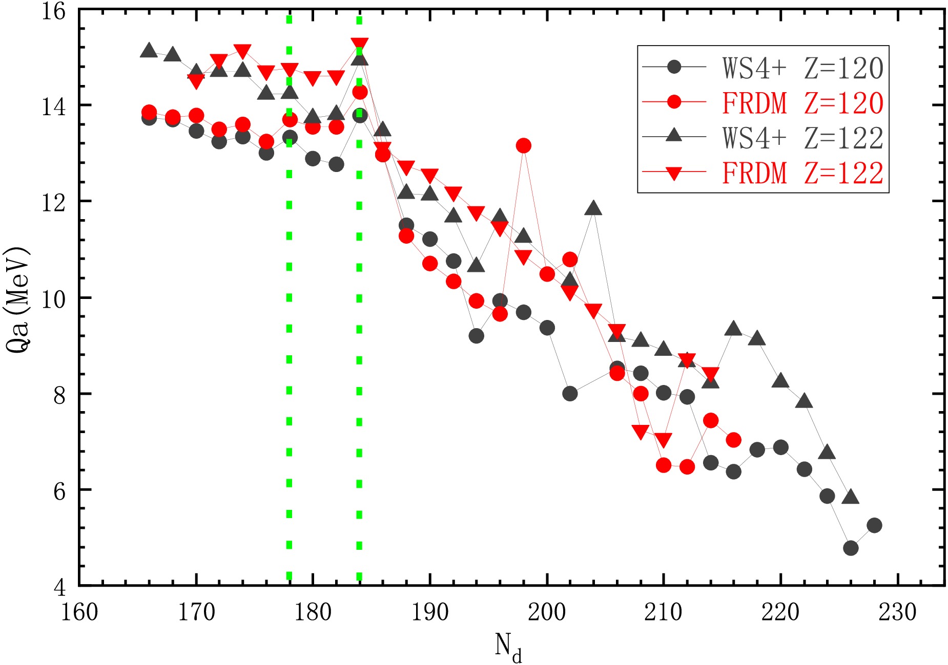
Figure 2. (color online) The predicted α decay energies
$Q_{\alpha}$ for even-even nuclei with$Z=120$ and 122 as functions of the neutron number$N_d$ of the daughter nucleus. The different symbols denote the results obtained from the WS4+ and FRDM mass models.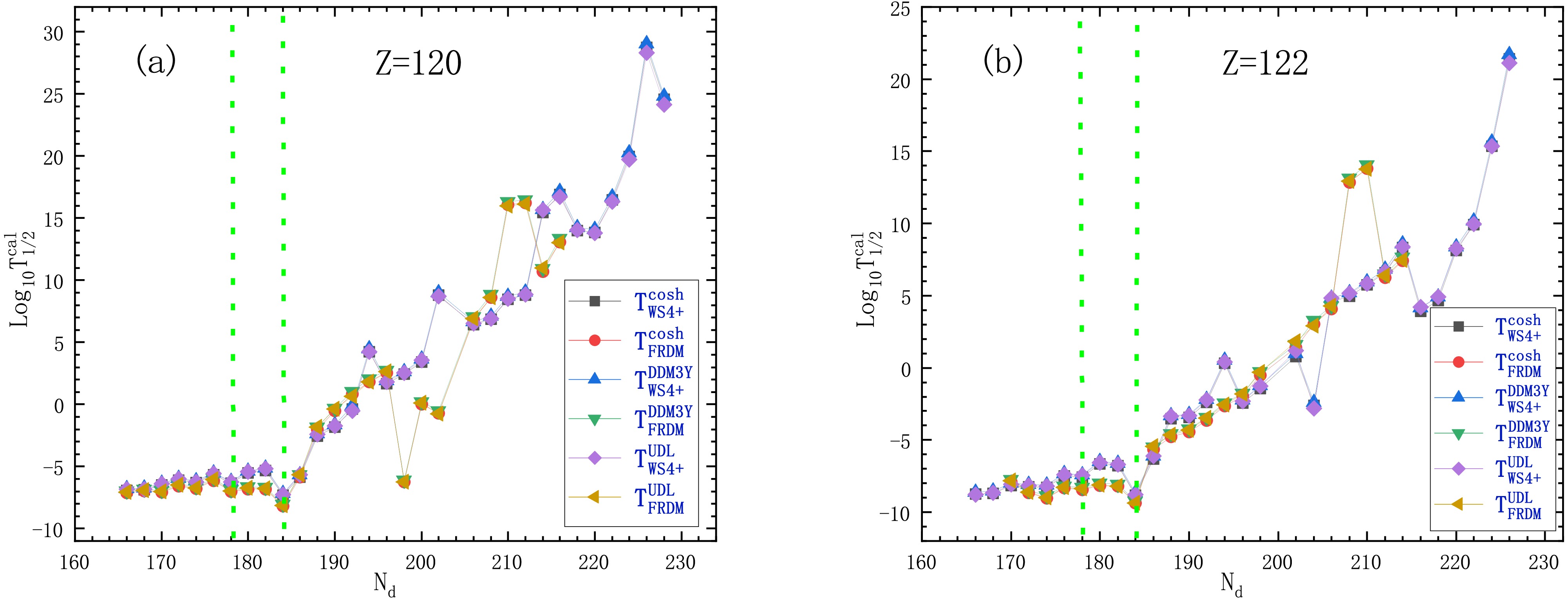
Figure 3. (color online) The predicted α-decay half-lives, in logarithmic form, of even-even nuclei with Z = 120 and 122. Different symbol types denote the results obtained using various nuclear potentials (Cosh or DDM3Y) and mass models (WS4+ or FRDM). The corresponding UDL predictions are also shown for comparison.
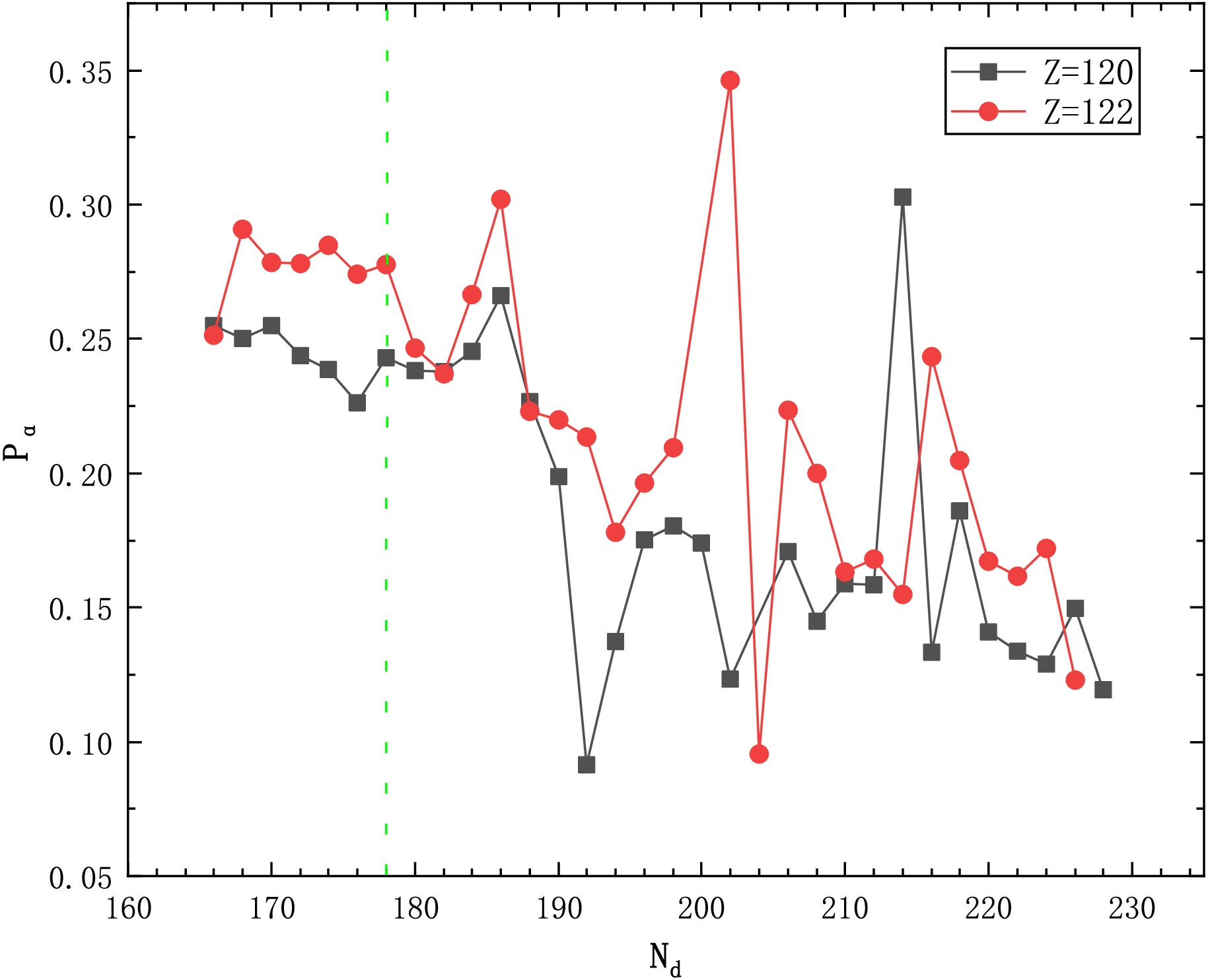
Figure 4. (color online) The CFM calculated preformation factors
$P_\alpha$ of$Z = 120$ and$ Z = 122$ plotted as a function of$N_d$ . -
We first combine the transition matrix method with the CFM to systematically calculate the α-decay half-lives of 177 even-even nuclei. To evaluate the accuracy of this model, we calculate the RMS deviation, which is defined as
$ \sigma = \left[ \frac{1}{n} \sum\limits_{i=1}^{n} \left( \log_{10} T_{1/2}^{\mathrm{exp}} - \log_{10} T_{1/2}^{\mathrm{cal}} \right)^2 \right]^{1/2}, $
(50) where
$ \log_{10} T_{1/2}^{\mathrm{exp}} $ and$ \log_{10} T_{1/2}^{\mathrm{cal}} $ are the logarithms of the experimental and calculated α-decay half-lives, respectively. In the spherical cosh-potential calculation, we determine the nuclear potential in Eq. (31) by fitting to the experimental half-lives of 177 even-even nuclei. The optimized parameters are$ V_0 $ = 186.25$ \mathrm{MeV} $ and a = 0.6719$ \mathrm{fm} $ . In this work, we use the transition matrix method instead of the traditional WKB approximation to calculate the penetration probability. Its main strength is that it can treat arbitrarily shaped barriers and produce accurate tunneling probabilities within a quantum-mechanical framework. Another key advance of this work is the direct calculation of$ P_\alpha $ from nuclear binding energies using the CFM, without parameter fitting, thereby providing independent predictive capability. The obtained$ P_\alpha $ values range from 0.10 to 0.28. This differs from the approach of Wu et al. [57], in which$ P_\alpha $ is determined either as a fitted constant or from microscopic corrections to the nuclear mass.Specifically, we perform four independent calculations for the same set of 177 even-even nuclei to quantify the effects of deformation and of the total interaction potential. These four calculations correspond to the spherical cosh-potential scenario, the deformed cosh-potential scenario, the spherical microscopic DDM3Y double-folding potential scenario, and the deformed microscopic DDM3Y double-folding potential scenario, respectively. It is important to note that the two potentials treat deformation differently. In the cosh potential, although the sharp radius
$R(\theta)$ accounts for deformation, the depth$V_0$ and diffuseness a of the nuclear potential are optimized by fitting the experimental data within a spherical baseline. Therefore, in the deformed cosh calculations, the nuclear potential retains its spherically symmetric form, and the deformation-induced variation arises only from the Coulomb interaction. In the microscopic DDM3Y double-folding potential, deformation is introduced directly into the density distribution of the daughter nucleus, making both the nuclear and Coulomb potentials orientation-dependent.The corresponding RMS deviations are summarized in Table 1. As shown in Table 1, in the cosh-potential calculation, the inclusion of deformation reduces the RMS deviation from 0.375 to 0.370, corresponding to a 1.3% improvement. In the microscopic DDM3Y double-folding potential calculation, the inclusion of deformation decreases the RMS deviation from 0.380 to 0.362, corresponding to a 4.7% improvement. It is noteworthy that the spherical microscopic DDM3Y double-folding potential result is globally slightly less accurate than the fitted spherical cosh-potential result, although the two RMS deviations are very close. This indicates that replacing a phenomenological potential with a microscopic interaction does not automatically reduce the RMS deviation. Nevertheless, the microscopic DDM3Y double-folding potential provides a density-based and independently constrained description of the nuclear interaction. Moreover, among the four calculations, the deformed microscopic DDM3Y double-folding potential shows the best agreement with the experimental data.
Potential model Without deformation deformation cosh 0.375 0.370 DDM3Y 0.380 0.362 Table 1. Root-mean-square deviations, σ, between the calculated α-decay half-lives and the experimental data for 177 even-even nuclei.
The detailed numerical results are presented in Table 2. In this table, the first five columns denote the α transition, the decay energies
$Q_{\alpha}$ , the preformation factors$P_{\alpha}$ calculated using the CFM, and the quadrupole ($\beta_2$ ) and hexadecapole ($\beta_4$ ) deformation parameters taken from the FRDM mass table. The next five columns show the experimental half-lives$T^{\mathrm{exp}}_{1/2}$ and the calculated half-lives obtained using the cosh potential and the microscopic DDM3Y double-folding potential under both spherical and deformation-averaged calculations, respectively. For a more intuitive comparison, the experimental data and calculated results are plotted on a logarithmic scale in Fig. 1. As shown in this figure, the four calculations exhibit a similar overall dependence on the parent mass number, and most logarithmic deviations remain within the interval from$ -0.5 $ to$ 0.5 $ . However, two conspicuous outliers appear at$ ^{268}\text{Hs} $ ($ Z = 108 $ ,$ N = 160 $ ) and$ ^{282}\text{Ds} $ ($ Z = 110 $ ,$ N = 172 $ ), where the deviations exceed one order of magnitude.
Figure 1. (color online) Logarithmic of deviations between the calculated half-lives and experimental data as a function of mass numbers. The results obtained with the spherical and deformed cosh and DDM3Y potentials are shown by different symbols.
α transition $Q_{\alpha}$ $P_{\alpha}$ $\beta_2$ $\beta_4$ $T_{1/2}^{\text{exp}}$ $T_{1/2}^{\text{Cosh}}$ $T_{1/2}^{\text{Cosh, Def.}}$ $T_{1/2}^{\text{DDM3Y}}$ $T_{1/2}^{\text{DDM3Y, Def.}}$ $^{146}\text{Sm}\to^{142}\text{Nd}$ 2.529 0.198 0.000 0.000 $2.15\times10^{15}$ $7.37\times10^{15}$ $7.37\times10^{15}$ $4.85\times10^{15}$ $4.85\times10^{15}$ $^{148}\text{Sm}\to^{144}\text{Nd}$ 1.987 0.195 0.000 0.000 $1.99\times10^{23}$ $1.03\times10^{24}$ $1.03\times10^{24}$ $6.64\times10^{23}$ $6.64\times10^{23}$ $^{148}\text{Gd}\to^{144}\text{Sm}$ 3.271 0.202 0.000 0.000 $2.25\times10^{9}$ $3.90\times10^{9}$ $3.90\times10^{9}$ $2.68\times10^{9}$ $2.68\times10^{9}$ $^{150}\text{Gd}\to^{146}\text{Sm}$ 2.807 0.202 0.000 0.000 $5.65\times10^{13}$ $1.36\times10^{14}$ $1.36\times10^{14}$ $9.27\times10^{13}$ $9.27\times10^{13}$ $^{152}\text{Gd}\to^{148}\text{Sm}$ 2.204 0.221 0.172 0.060 $3.41\times10^{21}$ $1.24\times10^{22}$ $1.18\times10^{22}$ $8.26\times10^{21}$ $5.48\times10^{21}$ $^{150}\text{Dy}\to^{146}\text{Gd}$ 4.351 0.236 0.000 0.000 $1.28\times10^{3}$ $1.13\times10^{3}$ $1.13\times10^{3}$ $8.12\times10^{2}$ $8.12\times10^{2}$ $^{152}\text{Dy}\to^{148}\text{Gd}$ 3.726 0.240 0.000 0.000 $8.51\times10^{6}$ $1.35\times10^{7}$ $1.35\times10^{7}$ $9.62\times10^{6}$ $9.62\times10^{6}$ $^{154}\text{Dy}\to^{150}\text{Gd}$ 2.945 0.238 0.172 0.047 $9.47\times10^{13}$ $1.13\times10^{14}$ $1.07\times10^{14}$ $7.87\times10^{13}$ $5.52\times10^{13}$ $^{152}\text{Er}\to^{148}\text{Dy}$ 4.934 0.239 0.011 0.000 $1.14\times10^{1}$ $1.00\times10^{1}$ $1.00\times10^{1}$ $7.42\times10^{0}$ $7.41\times10^{0}$ $^{154}\text{Er}\to^{150}\text{Dy}$ 4.280 0.257 0.000 0.000 $4.75\times10^{4}$ $3.71\times10^{4}$ $3.71\times10^{4}$ $2.72\times10^{4}$ $2.72\times10^{4}$ $^{156}\text{Er}\to^{152}\text{Dy}$ 3.481 0.252 0.172 0.035 $9.75\times10^{9}$ $2.25\times10^{10}$ $2.12\times10^{10}$ $1.62\times10^{10}$ $1.18\times10^{10}$ $^{154}\text{Yb}\to^{150}\text{Er}$ 5.474 0.235 0.011 0.000 $4.42\times10^{-1}$ $3.23\times10^{-1}$ $3.23\times10^{-1}$ $2.45\times10^{-1}$ $2.45\times10^{-1}$ $^{156}\text{Yb}\to^{152}\text{Er}$ 4.809 0.257 −0.084 0.014 $2.56\times10^{2}$ $4.46\times10^{2}$ $4.38\times10^{2}$ $3.36\times10^{2}$ $3.21\times10^{2}$ $^{156}\text{Hf}\to^{152}\text{Yb}$ 6.025 0.270 0.000 0.000 $2.30\times10^{-2}$ $1.35\times10^{-2}$ $1.35\times10^{-2}$ $1.05\times10^{-2}$ $1.05\times10^{-2}$ $^{158}\text{Hf}\to^{154}\text{Yb}$ 5.405 0.246 −0.104 0.028 $6.43\times10^{0}$ $5.66\times10^{0}$ $5.51\times10^{0}$ $4.38\times10^{0}$ $4.05\times10^{0}$ $^{160}\text{Hf}\to^{156}\text{Yb}$ 4.902 0.255 0.139 0.044 $1.89\times10^{3}$ $1.57\times10^{3}$ $1.50\times10^{3}$ $1.21\times10^{3}$ $9.71\times10^{2}$ $^{162}\text{Hf}\to^{158}\text{Yb}$ 4.417 0.241 0.183 0.025 $4.86\times10^{5}$ $9.82\times10^{5}$ $9.14\times10^{5}$ $7.55\times10^{5}$ $5.42\times10^{5}$ $^{158}\text{W}\to^{154}\text{Hf}$ 6.615 0.241 0.021 0.000 $1.43\times10^{-3}$ $8.14\times10^{-4}$ $8.13\times10^{-4}$ $6.46\times10^{-4}$ $6.45\times10^{-4}$ $^{160}\text{W}\to^{156}\text{Hf}$ 6.065 0.273 −0.084 0.014 $1.03\times10^{-1}$ $7.09\times10^{-2}$ $6.96\times10^{-2}$ $5.63\times10^{-2}$ $5.38\times10^{-2}$ $^{162}\text{W}\to^{158}\text{Hf}$ 5.678 0.244 0.128 0.030 $2.63\times10^{0}$ $2.96\times10^{0}$ $2.85\times10^{0}$ $2.35\times10^{0}$ $2.01\times10^{0}$ $^{164}\text{W}\to^{160}\text{Hf}$ 5.278 0.251 0.161 0.022 $1.65\times10^{2}$ $1.89\times10^{2}$ $1.78\times10^{2}$ $1.50\times10^{2}$ $1.18\times10^{2}$ $^{166}\text{W}\to^{162}\text{Hf}$ 4.856 0.231 0.183 0.013 $5.47\times10^{4}$ $3.05\times10^{4}$ $2.83\times10^{4}$ $2.41\times10^{4}$ $1.78\times10^{4}$ $^{168}\text{W}\to^{164}\text{Hf}$ 4.500 0.236 0.206 0.016 $1.59\times10^{6}$ $3.52\times10^{6}$ $3.20\times10^{6}$ $2.77\times10^{6}$ $1.83\times10^{6}$ $^{180}\text{W}\to^{176}\text{Hf}$ 2.515 0.162 0.278 −0.057 $5.02\times10^{25}$ $5.67\times10^{25}$ $4.84\times10^{25}$ $4.34\times10^{25}$ $2.11\times10^{25}$ $^{162}\text{Os}\to^{158}\text{W}$ 6.765 0.237 0.085 0.003 $2.10\times10^{-3}$ $1.64\times10^{-3}$ $1.61\times10^{-3}$ $1.33\times10^{-3}$ $1.27\times10^{-3}$ $^{164}\text{Os}\to^{160}\text{W}$ 6.485 0.271 0.128 0.018 $2.18\times10^{-2}$ $1.29\times10^{-2}$ $1.23\times10^{-2}$ $1.05\times10^{-2}$ $9.16\times10^{-3}$ $^{166}\text{Os}\to^{162}\text{W}$ 6.142 0.247 0.150 0.020 $2.55\times10^{-1}$ $2.63\times10^{-1}$ $2.49\times10^{-1}$ $2.14\times10^{-1}$ $1.76\times10^{-1}$ $^{168}\text{Os}\to^{164}\text{W}$ 5.816 0.247 0.173 −0.001 $4.84\times10^{0}$ $5.46\times10^{0}$ $5.07\times10^{0}$ $4.44\times10^{0}$ $3.51\times10^{0}$ $^{170}\text{Os}\to^{166}\text{W}$ 5.536 0.237 0.184 0.001 $7.75\times10^{1}$ $9.52\times10^{1}$ $8.77\times10^{1}$ $7.74\times10^{1}$ $5.84\times10^{1}$ $^{172}\text{Os}\to^{168}\text{W}$ 5.224 0.240 0.206 −0.009 $1.61\times10^{3}$ $2.92\times10^{3}$ $2.64\times10^{3}$ $2.38\times10^{3}$ $1.67\times10^{3}$ $^{174}\text{Os}\to^{170}\text{W}$ 4.871 0.226 0.217 −0.007 $1.78\times10^{5}$ $2.32\times10^{5}$ $2.08\times10^{5}$ $1.89\times10^{5}$ $1.25\times10^{5}$ $^{186}\text{Os}\to^{182}\text{W}$ 2.821 0.157 0.232 −0.066 $6.31\times10^{22}$ $9.44\times10^{22}$ $8.37\times10^{22}$ $7.50\times10^{22}$ $4.44\times10^{22}$ $^{166}\text{Pt}\to^{162}\text{Os}$ 7.295 0.238 0.107 −0.008 $2.94\times10^{-4}$ $1.81\times10^{-4}$ $1.75\times10^{-4}$ $1.50\times10^{-4}$ $1.39\times10^{-4}$ $^{168}\text{Pt}\to^{164}\text{Os}$ 6.985 0.272 0.129 0.006 $2.02\times10^{-3}$ $1.45\times10^{-3}$ $1.39\times10^{-3}$ $1.21\times10^{-3}$ $1.07\times10^{-3}$ $^{170}\text{Pt}\to^{166}\text{Os}$ 6.708 0.242 0.151 −0.004 $1.39\times10^{-2}$ $1.35\times10^{-2}$ $1.28\times10^{-2}$ $1.13\times10^{-2}$ $9.56\times10^{-3}$ $^{172}\text{Pt}\to^{168}\text{Os}$ 6.463 0.254 0.173 −0.013 $1.01\times10^{-1}$ $9.33\times10^{-2}$ $8.63\times10^{-2}$ $7.79\times10^{-2}$ $6.25\times10^{-2}$ $^{174}\text{Pt}\to^{170}\text{Os}$ 6.183 0.247 0.184 −0.012 $1.15\times10^{0}$ $1.09\times10^{0}$ $1.00\times10^{0}$ $9.15\times10^{-1}$ $6.98\times10^{-1}$ $^{176}\text{Pt}\to^{172}\text{Os}$ 5.885 0.261 0.195 −0.010 $1.57\times10^{1}$ $1.72\times10^{1}$ $1.56\times10^{1}$ $1.44\times10^{1}$ $1.06\times10^{1}$ $^{178}\text{Pt}\to^{174}\text{Os}$ 5.573 0.227 0.217 −0.007 $2.68\times10^{2}$ $4.83\times10^{2}$ $4.30\times10^{2}$ $4.04\times10^{2}$ $2.69\times10^{2}$ $^{180}\text{Pt}\to^{176}\text{Os}$ 5.276 0.205 0.218 −0.019 $1.07\times10^{4}$ $1.47\times10^{4}$ $1.31\times10^{4}$ $1.23\times10^{4}$ $8.22\times10^{3}$ $^{182}\text{Pt}\to^{178}\text{Os}$ 4.951 0.187 0.219 −0.031 $4.19\times10^{5}$ $8.79\times10^{5}$ $7.81\times10^{5}$ $7.36\times10^{5}$ $4.89\times10^{5}$ $^{184}\text{Pt}\to^{180}\text{Os}$ 4.599 0.186 0.219 −0.043 $5.86\times10^{7}$ $1.11\times10^{8}$ $9.87\times10^{7}$ $9.29\times10^{7}$ $6.13\times10^{7}$ $^{186}\text{Pt}\to^{182}\text{Os}$ 4.320 0.173 0.220 −0.056 $5.35\times10^{9}$ $8.29\times10^{9}$ $7.36\times10^{9}$ $6.92\times10^{9}$ $4.51\times10^{9}$ $^{188}\text{Pt}\to^{184}\text{Os}$ 4.007 0.216 0.220 −0.068 $3.38\times10^{12}$ $1.36\times10^{12}$ $1.21\times10^{12}$ $1.14\times10^{12}$ $7.26\times10^{11}$ $^{190}\text{Pt}\to^{186}\text{Os}$ 3.269 0.203 0.209 −0.083 $1.52\times10^{19}$ $9.46\times10^{18}$ $8.50\times10^{18}$ $7.80\times10^{18}$ $4.95\times10^{18}$ $^{172}\text{Hg}\to^{168}\text{Pt}$ 7.525 0.277 0.118 0.005 $2.31\times10^{-4}$ $1.55\times10^{-4}$ $1.49\times10^{-4}$ $1.31\times10^{-4}$ $1.19\times10^{-4}$ $^{174}\text{Hg}\to^{170}\text{Pt}$ 7.233 0.249 0.129 −0.006 $2.00\times10^{-3}$ $1.31\times10^{-3}$ $1.25\times10^{-3}$ $1.12\times10^{-3}$ $9.94\times10^{-4}$ $^{176}\text{Hg}\to^{172}\text{Pt}$ 6.897 0.267 0.140 −0.005 $2.23\times10^{-2}$ $1.53\times10^{-2}$ $1.45\times10^{-2}$ $1.31\times10^{-2}$ $1.13\times10^{-2}$ $^{178}\text{Hg}\to^{174}\text{Pt}$ 6.577 0.258 0.162 −0.003 $2.98\times10^{-1}$ $2.12\times10^{-1}$ $1.98\times10^{-1}$ $1.82\times10^{-1}$ $1.47\times10^{-1}$ $^{180}\text{Hg}\to^{176}\text{Pt}$ 6.258 0.265 0.239 0.021 $5.37\times10^{0}$ $3.42\times10^{0}$ $2.96\times10^{0}$ $2.93\times10^{0}$ $1.66\times10^{0}$ $^{182}\text{Hg}\to^{178}\text{Pt}$ 5.995 0.254 0.250 0.011 $7.80\times10^{1}$ $4.23\times10^{1}$ $3.61\times10^{1}$ $3.63\times10^{1}$ $1.99\times10^{1}$ $^{184}\text{Hg}\to^{180}\text{Pt}$ 5.660 0.242 0.251 −0.002 $2.77\times10^{3}$ $1.39\times10^{3}$ $1.19\times10^{3}$ $1.20\times10^{3}$ $6.63\times10^{2}$ $^{186}\text{Hg}\to^{182}\text{Pt}$ 5.204 0.247 0.219 −0.031 $5.02\times10^{5}$ $2.68\times10^{5}$ $2.37\times10^{5}$ $2.31\times10^{5}$ $1.52\times10^{5}$ $^{188}\text{Hg}\to^{184}\text{Pt}$ 4.709 0.239 0.219 −0.044 $5.27\times10^{8}$ $2.12\times10^{8}$ $1.87\times10^{8}$ $1.82\times10^{8}$ $1.18\times10^{8}$ $^{180}\text{Pb}\to^{176}\text{Hg}$ 7.419 0.248 −0.115 −0.030 $4.10\times10^{-3}$ $1.74\times10^{-3}$ $1.66\times10^{-3}$ $1.52\times10^{-3}$ $1.41\times10^{-3}$ $^{182}\text{Pb}\to^{178}\text{Hg}$ 7.065 0.234 −0.125 −0.017 $5.50\times10^{-2}$ $2.57\times10^{-2}$ $2.44\times10^{-2}$ $2.26\times10^{-2}$ $2.06\times10^{-2}$ $^{184}\text{Pb}\to^{180}\text{Hg}$ 6.774 0.236 −0.135 −0.005 $6.12\times10^{-1}$ $2.59\times10^{-1}$ $2.44\times10^{-1}$ $2.28\times10^{-1}$ $2.03\times10^{-1}$ $^{186}\text{Pb}\to^{182}\text{Hg}$ 6.471 0.230 −0.146 −0.004 $1.18\times10^{1}$ $3.56\times10^{0}$ $3.32\times10^{0}$ $3.14\times10^{0}$ $2.74\times10^{0}$ $^{188}\text{Pb}\to^{184}\text{Hg}$ 6.109 0.221 −0.146 −0.004 $2.94\times10^{2}$ $1.10\times10^{2}$ $1.02\times10^{2}$ $9.71\times10^{1}$ $8.42\times10^{1}$ $^{190}\text{Pb}\to^{186}\text{Hg}$ 5.697 0.216 −0.146 −0.004 $1.76\times10^{4}$ $8.24\times10^{3}$ $7.69\times10^{3}$ $7.29\times10^{3}$ $6.28\times10^{3}$ $^{192}\text{Pb}\to^{188}\text{Hg}$ 5.221 0.204 −0.146 −0.015 $3.52\times10^{6}$ $2.42\times10^{6}$ $2.26\times10^{6}$ $2.14\times10^{6}$ $1.84\times10^{6}$ $^{194}\text{Pb}\to^{190}\text{Hg}$ 4.738 0.195 −0.125 −0.017 $8.79\times10^{9}$ $1.86\times10^{9}$ $1.77\times10^{9}$ $1.65\times10^{9}$ $1.46\times10^{9}$ $^{210}\text{Pb}\to^{206}\text{Hg}$ 3.793 0.107 0.000 0.000 $3.69\times10^{16}$ $2.85\times10^{16}$ $2.85\times10^{16}$ $2.54\times10^{16}$ $2.54\times10^{16}$ $^{188}\text{Po}\to^{184}\text{Pb}$ 8.083 0.275 0.000 0.012 $2.70\times10^{-4}$ $6.48\times10^{-5}$ $6.48\times10^{-5}$ $5.80\times10^{-5}$ $5.79\times10^{-5}$ $^{190}\text{Po}\to^{186}\text{Pb}$ 7.693 0.262 0.000 0.000 $2.45\times10^{-3}$ $9.22\times10^{-4}$ $9.22\times10^{-4}$ $8.30\times10^{-4}$ $8.30\times10^{-4}$ $^{192}\text{Po}\to^{188}\text{Pb}$ 7.320 0.257 0.000 0.000 $3.22\times10^{-2}$ $1.40\times10^{-2}$ $1.40\times10^{-2}$ $1.26\times10^{-2}$ $1.26\times10^{-2}$ $^{194}\text{Po}\to^{190}\text{Pb}$ 6.987 0.235 0.000 0.000 $3.92\times10^{-1}$ $2.05\times10^{-1}$ $2.05\times10^{-1}$ $1.86\times10^{-1}$ $1.86\times10^{-1}$ $^{196}\text{Po}\to^{192}\text{Pb}$ 6.658 0.216 0.000 0.000 $5.96\times10^{0}$ $3.56\times10^{0}$ $3.56\times10^{0}$ $3.24\times10^{0}$ $3.24\times10^{0}$ $^{198}\text{Po}\to^{194}\text{Pb}$ 6.310 0.203 0.000 0.000 $1.85\times10^{2}$ $9.17\times10^{1}$ $9.17\times10^{1}$ $8.36\times10^{1}$ $8.36\times10^{1}$ $^{200}\text{Po}\to^{196}\text{Pb}$ 5.981 0.184 0.000 0.000 $6.20\times10^{3}$ $2.69\times10^{3}$ $2.69\times10^{3}$ $2.46\times10^{3}$ $2.46\times10^{3}$ $^{202}\text{Po}\to^{198}\text{Pb}$ 5.700 0.177 0.000 0.000 $1.39\times10^{5}$ $5.75\times10^{4}$ $5.75\times10^{4}$ $5.26\times10^{4}$ $5.26\times10^{4}$ $^{204}\text{Po}\to^{200}\text{Pb}$ 5.485 0.158 0.000 0.000 $1.88\times10^{6}$ $7.49\times10^{5}$ $7.49\times10^{5}$ $6.87\times10^{5}$ $6.87\times10^{5}$ $^{206}\text{Po}\to^{202}\text{Pb}$ 5.327 0.145 0.000 0.000 $1.39\times10^{7}$ $5.33\times10^{6}$ $5.33\times10^{6}$ $4.90\times10^{6}$ $4.90\times10^{6}$ $^{208}\text{Po}\to^{204}\text{Pb}$ 5.216 0.135 0.000 0.000 $9.15\times10^{7}$ $2.21\times10^{7}$ $2.21\times10^{7}$ $2.04\times10^{7}$ $2.04\times10^{7}$ $^{210}\text{Po}\to^{206}\text{Pb}$ 5.407 0.106 0.000 0.000 $1.20\times10^{7}$ $2.17\times10^{6}$ $2.17\times10^{6}$ $2.00\times10^{6}$ $2.00\times10^{6}$ $^{212}\text{Po}\to^{208}\text{Pb}$ 8.954 0.221 0.000 0.000 $2.94\times10^{-7}$ $1.19\times10^{-7}$ $1.19\times10^{-7}$ $1.09\times10^{-7}$ $1.09\times10^{-7}$ $^{214}\text{Po}\to^{210}\text{Pb}$ 7.833 0.213 0.000 0.000 $1.63\times10^{-4}$ $1.30\times10^{-4}$ $1.30\times10^{-4}$ $1.20\times10^{-4}$ $1.20\times10^{-4}$ $^{216}\text{Po}\to^{212}\text{Pb}$ 6.906 0.205 0.000 0.000 $1.44\times10^{-1}$ $1.60\times10^{-1}$ $1.60\times10^{-1}$ $1.49\times10^{-1}$ $1.49\times10^{-1}$ $^{218}\text{Po}\to^{214}\text{Pb}$ 6.115 0.196 0.000 0.000 $1.86\times10^{2}$ $2.58\times10^{2}$ $2.58\times10^{2}$ $2.41\times10^{2}$ $2.41\times10^{2}$ $^{194}\text{Rn}\to^{190}\text{Po}$ 7.863 0.261 −0.217 0.017 $7.80\times10^{-4}$ $1.51\times10^{-3}$ $1.27\times10^{-3}$ $1.39\times10^{-3}$ $1.04\times10^{-3}$ $^{196}\text{Rn}\to^{192}\text{Po}$ 7.616 0.256 −0.217 0.017 $4.70\times10^{-3}$ $8.53\times10^{-3}$ $7.16\times10^{-3}$ $7.89\times10^{-3}$ $5.83\times10^{-3}$ $^{198}\text{Rn}\to^{194}\text{Po}$ 7.350 0.239 −0.207 0.015 $6.87\times10^{-2}$ $6.48\times10^{-2}$ $5.53\times10^{-2}$ $6.02\times10^{-2}$ $4.53\times10^{-2}$ $^{200}\text{Rn}\to^{196}\text{Po}$ 7.044 0.221 0.085 0.003 $1.17\times10^{0}$ $7.86\times10^{-1}$ $7.68\times10^{-1}$ $7.32\times10^{-1}$ $6.86\times10^{-1}$ $^{202}\text{Rn}\to^{198}\text{Po}$ 6.773 0.209 0.075 0.002 $1.23\times10^{1}$ $8.10\times10^{0}$ $7.95\times10^{0}$ $7.57\times10^{0}$ $7.19\times10^{0}$ $^{204}\text{Rn}\to^{200}\text{Po}$ 6.547 0.191 −0.063 0.013 $1.03\times10^{2}$ $6.55\times10^{1}$ $6.46\times10^{1}$ $6.14\times10^{1}$ $6.05\times10^{1}$ $^{206}\text{Rn}\to^{202}\text{Po}$ 6.384 0.180 −0.063 0.001 $5.46\times10^{2}$ $3.07\times10^{2}$ $3.03\times10^{2}$ $2.89\times10^{2}$ $2.79\times10^{2}$ $^{208}\text{Rn}\to^{204}\text{Po}$ 6.261 0.163 −0.042 0.001 $2.33\times10^{3}$ $1.06\times10^{3}$ $1.06\times10^{3}$ $1.00\times10^{3}$ $9.88\times10^{2}$ $^{210}\text{Rn}\to^{206}\text{Po}$ 6.159 0.152 0.000 0.000 $8.99\times10^{3}$ $2.97\times10^{3}$ $2.97\times10^{3}$ $2.81\times10^{3}$ $2.81\times10^{3}$ $^{212}\text{Rn}\to^{208}\text{Po}$ 6.385 0.121 0.000 0.000 $1.43\times10^{3}$ $3.38\times10^{2}$ $3.38\times10^{2}$ $3.20\times10^{2}$ $3.20\times10^{2}$ $^{214}\text{Rn}\to^{210}\text{Po}$ 9.208 0.229 0.000 0.000 $2.59\times10^{-7}$ $1.36\times10^{-7}$ $1.36\times10^{-7}$ $1.27\times10^{-7}$ $1.27\times10^{-7}$ $^{216}\text{Rn}\to^{212}\text{Po}$ 8.197 0.237 0.000 0.000 $2.90\times10^{-5}$ $5.64\times10^{-5}$ $5.64\times10^{-5}$ $5.32\times10^{-5}$ $5.32\times10^{-5}$ $^{218}\text{Rn}\to^{214}\text{Po}$ 7.262 0.234 0.000 0.000 $3.38\times10^{-2}$ $5.04\times10^{-2}$ $5.04\times10^{-2}$ $4.79\times10^{-2}$ $4.79\times10^{-2}$ $^{220}\text{Rn}\to^{216}\text{Po}$ 6.405 0.221 0.000 0.000 $5.56\times10^{1}$ $1.04\times10^{2}$ $1.04\times10^{2}$ $9.91\times10^{1}$ $9.91\times10^{1}$ $^{222}\text{Rn}\to^{218}\text{Po}$ 5.590 0.222 0.056 0.028 $3.30\times10^{5}$ $7.04\times10^{5}$ $6.97\times10^{5}$ $6.75\times10^{5}$ $6.38\times10^{5}$ $^{202}\text{Ra}\to^{198}\text{Rn}$ 7.880 0.248 −0.227 0.019 $4.10\times10^{-3}$ $6.33\times10^{-3}$ $5.19\times10^{-3}$ $6.02\times10^{-3}$ $4.29\times10^{-3}$ $^{204}\text{Ra}\to^{200}\text{Rn}$ 7.636 0.231 −0.207 0.004 $6.00\times10^{-2}$ $3.83\times10^{-2}$ $3.24\times10^{-2}$ $3.65\times10^{-2}$ $2.77\times10^{-2}$ $^{206}\text{Ra}\to^{202}\text{Rn}$ 7.416 0.219 −0.115 0.017 $2.40\times10^{-1}$ $2.07\times10^{-1}$ $1.97\times10^{-1}$ $1.98\times10^{-1}$ $1.78\times10^{-1}$ $^{208}\text{Ra}\to^{204}\text{Rn}$ 7.273 0.195 −0.115 0.017 $1.27\times10^{0}$ $6.73\times10^{-1}$ $6.41\times10^{-1}$ $6.46\times10^{-1}$ $5.79\times10^{-1}$ $^{210}\text{Ra}\to^{206}\text{Rn}$ 7.151 0.187 −0.094 0.015 $4.00\times10^{0}$ $1.78\times10^{0}$ $1.72\times10^{0}$ $1.71\times10^{0}$ $1.59\times10^{0}$ $^{214}\text{Ra}\to^{210}\text{Rn}$ 7.273 0.138 0.000 0.000 $2.44\times10^{0}$ $7.08\times10^{-1}$ $7.08\times10^{-1}$ $6.85\times10^{-1}$ $6.85\times10^{-1}$ $^{216}\text{Ra}\to^{212}\text{Rn}$ 9.525 0.239 0.000 0.000 $1.72\times10^{-7}$ $1.09\times10^{-7}$ $1.09\times10^{-7}$ $1.04\times10^{-7}$ $1.04\times10^{-7}$ $^{218}\text{Ra}\to^{214}\text{Rn}$ 8.541 0.243 0.000 0.000 $2.59\times10^{-5}$ $3.21\times10^{-5}$ $3.21\times10^{-5}$ $3.09\times10^{-5}$ $3.09\times10^{-5}$ $^{220}\text{Ra}\to^{216}\text{Rn}$ 7.594 0.239 0.000 0.000 $1.81\times10^{-2}$ $2.35\times10^{-2}$ $2.35\times10^{-2}$ $2.28\times10^{-2}$ $2.28\times10^{-2}$ $^{222}\text{Ra}\to^{218}\text{Rn}$ 6.678 0.199 0.079 0.054 $3.36\times10^{1}$ $6.56\times10^{1}$ $6.42\times10^{1}$ $6.42\times10^{1}$ $5.52\times10^{1}$ $^{224}\text{Ra}\to^{220}\text{Rn}$ 5.789 0.184 0.110 0.068 $3.14\times10^{5}$ $7.84\times10^{5}$ $7.54\times10^{5}$ $7.71\times10^{5}$ $5.59\times10^{5}$ $^{226}\text{Ra}\to^{222}\text{Rn}$ 4.871 0.182 0.110 0.068 $5.05\times10^{10}$ $1.75\times10^{11}$ $1.69\times10^{11}$ $1.73\times10^{11}$ $1.22\times10^{11}$ $^{210}\text{Th}\to^{206}\text{Ra}$ 8.069 0.234 −0.125 0.018 $1.60\times10^{-2}$ $7.59\times10^{-3}$ $7.14\times10^{-3}$ $7.43\times10^{-3}$ $6.57\times10^{-3}$ $^{212}\text{Th}\to^{208}\text{Ra}$ 7.958 0.196 −0.125 0.018 $3.17\times10^{-2}$ $1.85\times10^{-2}$ $1.74\times10^{-2}$ $1.82\times10^{-2}$ $1.60\times10^{-2}$ $^{214}\text{Th}\to^{210}\text{Ra}$ 7.827 0.195 −0.084 −0.009 $8.70\times10^{-2}$ $4.48\times10^{-2}$ $4.36\times10^{-2}$ $4.41\times10^{-2}$ $4.19\times10^{-2}$ $^{216}\text{Th}\to^{212}\text{Ra}$ 8.073 0.159 −0.053 −0.011 $2.63\times10^{-2}$ $8.13\times10^{-3}$ $8.04\times10^{-3}$ $8.00\times10^{-3}$ $7.83\times10^{-3}$ $^{218}\text{Th}\to^{214}\text{Ra}$ 9.849 0.251 0.000 0.000 $1.22\times10^{-7}$ $8.54\times10^{-8}$ $8.54\times10^{-8}$ $8.27\times10^{-8}$ $8.27\times10^{-8}$ $^{220}\text{Th}\to^{216}\text{Ra}$ 8.974 0.243 0.000 0.000 $1.02\times10^{-5}$ $1.12\times10^{-5}$ $1.12\times10^{-5}$ $1.10\times10^{-5}$ $1.10\times10^{-5}$ $^{222}\text{Th}\to^{218}\text{Ra}$ 8.132 0.232 0.078 0.054 $2.24\times10^{-3}$ $2.73\times10^{-3}$ $2.67\times10^{-3}$ $2.71\times10^{-3}$ $2.36\times10^{-3}$ $^{224}\text{Th}\to^{220}\text{Ra}$ 7.299 0.198 0.111 0.081 $1.04\times10^{0}$ $1.86\times10^{0}$ $1.78\times10^{0}$ $1.86\times10^{0}$ $1.30\times10^{0}$ $^{226}\text{Th}\to^{222}\text{Ra}$ 6.453 0.182 0.122 0.082 $1.84\times10^{3}$ $4.77\times10^{3}$ $4.54\times10^{3}$ $4.81\times10^{3}$ $3.10\times10^{3}$ $^{228}\text{Th}\to^{224}\text{Ra}$ 5.520 0.183 0.143 0.084 $6.04\times10^{7}$ $2.06\times10^{8}$ $1.93\times10^{8}$ $2.08\times10^{8}$ $1.14\times10^{8}$ $^{230}\text{Th}\to^{226}\text{Ra}$ 4.770 0.183 0.164 0.098 $2.38\times10^{12}$ $1.06\times10^{13}$ $9.75\times10^{12}$ $1.07\times10^{13}$ $4.38\times10^{12}$ $^{232}\text{Th}\to^{228}\text{Ra}$ 4.082 0.160 0.174 0.099 $4.42\times10^{17}$ $3.42\times10^{18}$ $3.13\times10^{18}$ $3.47\times10^{18}$ $1.23\times10^{18}$ $^{218}\text{U}\to^{214}\text{Th}$ 8.775 0.188 −0.063 −0.022 $3.54\times10^{-4}$ $3.19\times10^{-4}$ $3.14\times10^{-4}$ $3.20\times10^{-4}$ $3.10\times10^{-4}$ $^{222}\text{U}\to^{218}\text{Th}$ 9.478 0.245 0.000 0.000 $4.70\times10^{-6}$ $2.83\times10^{-6}$ $2.83\times10^{-6}$ $2.82\times10^{-6}$ $2.82\times10^{-6}$ $^{224}\text{U}\to^{220}\text{Th}$ 8.628 0.247 0.090 0.055 $3.96\times10^{-4}$ $4.79\times10^{-4}$ $4.65\times10^{-4}$ $4.84\times10^{-4}$ $4.09\times10^{-4}$ $^{226}\text{U}\to^{222}\text{Th}$ 7.701 0.208 0.111 0.069 $2.69\times10^{-1}$ $4.36\times10^{-1}$ $4.17\times10^{-1}$ $4.46\times10^{-1}$ $3.30\times10^{-1}$ $^{228}\text{U}\to^{224}\text{Th}$ 6.799 0.190 0.144 0.084 $5.60\times10^{2}$ $1.17\times10^{3}$ $1.09\times10^{3}$ $1.21\times10^{3}$ $6.84\times10^{2}$ $^{230}\text{U}\to^{226}\text{Th}$ 5.992 0.187 0.154 0.085 $1.75\times10^{6}$ $5.86\times10^{6}$ $5.43\times10^{6}$ $6.09\times10^{6}$ $3.10\times10^{6}$ $^{232}\text{U}\to^{228}\text{Th}$ 5.414 0.169 0.174 0.100 $2.17\times10^{9}$ $9.24\times10^{9}$ $8.41\times10^{9}$ $9.64\times10^{9}$ $3.64\times10^{9}$ $^{234}\text{U}\to^{230}\text{Th}$ 4.858 0.150 0.195 0.114 $7.75\times10^{12}$ $3.83\times10^{13}$ $3.42\times10^{13}$ $4.00\times10^{13}$ $1.06\times10^{13}$ $^{236}\text{U}\to^{232}\text{Th}$ 4.573 0.153 0.205 0.103 $7.39\times10^{14}$ $4.32\times10^{15}$ $3.82\times10^{15}$ $4.53\times10^{15}$ $1.19\times10^{15}$ $^{238}\text{U}\to^{234}\text{Th}$ 4.270 0.137 0.226 0.095 $1.41\times10^{17}$ $1.30\times10^{18}$ $1.12\times10^{18}$ $1.36\times10^{18}$ $3.10\times10^{17}$ $^{230}\text{Pu}\to^{226}\text{U}$ 7.178 0.201 0.143 0.084 $1.05\times10^{2}$ $2.35\times10^{2}$ $2.19\times10^{2}$ $2.49\times10^{2}$ $1.41\times10^{2}$ $^{232}\text{Pu}\to^{228}\text{U}$ 6.716 0.165 0.186 0.126 $1.01\times10^{4}$ $2.18\times10^{4}$ $1.94\times10^{4}$ $2.31\times10^{4}$ $6.74\times10^{3}$ $^{234}\text{Pu}\to^{230}\text{U}$ 6.310 0.152 0.185 0.126 $5.28\times10^{5}$ $1.57\times10^{6}$ $1.41\times10^{6}$ $1.68\times10^{6}$ $4.74\times10^{5}$ $^{236}\text{Pu}\to^{232}\text{U}$ 5.867 0.140 0.206 0.116 $9.02\times10^{7}$ $2.82\times10^{8}$ $2.47\times10^{8}$ $3.03\times10^{8}$ $7.56\times10^{7}$ $^{238}\text{Pu}\to^{234}\text{U}$ 5.593 0.145 0.215 0.106 $2.77\times10^{9}$ $8.46\times10^{9}$ $7.33\times10^{9}$ $9.12\times10^{9}$ $2.25\times10^{9}$ $^{240}\text{Pu}\to^{236}\text{U}$ 5.256 0.129 0.226 0.108 $2.07\times10^{11}$ $9.83\times10^{11}$ $8.41\times10^{11}$ $1.06\times10^{12}$ $2.24\times10^{11}$ $^{242}\text{Pu}\to^{238}\text{U}$ 4.984 0.133 0.236 0.098 $1.18\times10^{13}$ $5.60\times10^{13}$ $4.74\times10^{13}$ $6.07\times10^{13}$ $1.25\times10^{13}$ $^{244}\text{Pu}\to^{240}\text{U}$ 4.666 0.127 0.237 0.086 $2.57\times10^{15}$ $1.13\times10^{16}$ $9.54\times10^{15}$ $1.23\times10^{16}$ $2.71\times10^{15}$ $^{234}\text{Cm}\to^{230}\text{Pu}$ 7.365 0.194 0.195 0.114 $1.93\times10^{2}$ $2.91\times10^{2}$ $2.56\times10^{2}$ $3.16\times10^{2}$ $9.75\times10^{1}$ $^{236}\text{Cm}\to^{232}\text{Pu}$ 7.067 0.157 0.206 0.116 $2.24\times10^{3}$ $5.09\times10^{3}$ $4.42\times10^{3}$ $5.56\times10^{3}$ $1.50\times10^{3}$ $^{238}\text{Cm}\to^{234}\text{Pu}$ 6.670 0.137 0.216 0.119 $2.06\times10^{5}$ $2.78\times10^{5}$ $2.39\times10^{5}$ $3.05\times10^{5}$ $7.01\times10^{4}$ $^{240}\text{Cm}\to^{236}\text{Pu}$ 6.398 0.137 0.215 0.106 $2.63\times10^{6}$ $4.71\times10^{6}$ $4.05\times10^{6}$ $5.19\times10^{6}$ $1.33\times10^{6}$ $^{242}\text{Cm}\to^{238}\text{Pu}$ 6.216 0.122 0.226 0.095 $1.41\times10^{7}$ $3.81\times10^{7}$ $3.23\times10^{7}$ $4.22\times10^{7}$ $1.07\times10^{7}$ $^{244}\text{Cm}\to^{240}\text{Pu}$ 5.902 0.144 0.237 0.086 $5.71\times10^{8}$ $1.31\times10^{9}$ $1.10\times10^{9}$ $1.46\times10^{9}$ $3.54\times10^{8}$ $^{246}\text{Cm}\to^{242}\text{Pu}$ 5.475 0.142 0.237 0.073 $1.49\times10^{11}$ $3.59\times10^{11}$ $3.00\times10^{11}$ $4.01\times10^{11}$ $1.05\times10^{11}$ $^{248}\text{Cm}\to^{244}\text{Pu}$ 5.162 0.146 0.237 0.061 $1.20\times10^{13}$ $3.27\times10^{13}$ $2.74\times10^{13}$ $3.66\times10^{13}$ $1.03\times10^{13}$ $^{238}\text{Cf}\to^{234}\text{Cm}$ 8.133 0.185 0.205 0.103 $8.39\times10^{-1}$ $2.95\times10^{0}$ $2.55\times10^{0}$ $3.27\times10^{0}$ $1.06\times10^{0}$ $^{240}\text{Cf}\to^{236}\text{Cm}$ 7.711 0.150 0.215 0.106 $4.09\times10^{1}$ $1.03\times10^{2}$ $8.82\times10^{1}$ $1.16\times10^{2}$ $3.22\times10^{1}$ $^{242}\text{Cf}\to^{238}\text{Cm}$ 7.517 0.145 0.226 0.095 $3.42\times10^{2}$ $5.21\times10^{2}$ $4.38\times10^{2}$ $5.85\times10^{2}$ $1.62\times10^{2}$ $^{244}\text{Cf}\to^{240}\text{Cm}$ 7.329 0.153 0.237 0.085 $1.55\times10^{3}$ $2.46\times10^{3}$ $2.03\times10^{3}$ $2.77\times10^{3}$ $7.54\times10^{2}$ $^{246}\text{Cf}\to^{242}\text{Cm}$ 6.862 0.155 0.237 0.086 $1.29\times10^{5}$ $2.03\times10^{5}$ $1.68\times10^{5}$ $2.31\times10^{5}$ $5.90\times10^{4}$ $^{248}\text{Cf}\to^{244}\text{Cm}$ 6.361 0.138 0.249 0.063 $2.88\times10^{7}$ $4.62\times10^{7}$ $3.76\times10^{7}$ $5.28\times10^{7}$ $1.43\times10^{7}$ $^{250}\text{Cf}\to^{246}\text{Cm}$ 6.128 0.136 0.249 0.051 $4.13\times10^{8}$ $6.67\times10^{8}$ $5.43\times10^{8}$ $7.66\times10^{8}$ $2.24\times10^{8}$ $^{252}\text{Cf}\to^{248}\text{Cm}$ 6.217 0.146 0.250 0.039 $8.61\times10^{7}$ $1.95\times10^{8}$ $1.58\times10^{8}$ $2.24\times10^{8}$ $7.21\times10^{7}$ $^{254}\text{Cf}\to^{250}\text{Cm}$ 5.926 0.154 0.250 0.026 $1.68\times10^{9}$ $6.07\times10^{9}$ $4.92\times10^{9}$ $7.01\times10^{9}$ $2.41\times10^{9}$ $^{244}\text{Fm}\to^{240}\text{Cf}$ 8.546 0.166 0.237 0.085 $3.12\times10^{-1}$ $6.99\times10^{-1}$ $5.73\times10^{-1}$ $7.97\times10^{-1}$ $2.34\times10^{-1}$ $^{246}\text{Fm}\to^{242}\text{Cf}$ 8.379 0.154 0.237 0.073 $1.65\times10^{0}$ $2.40\times10^{0}$ $1.97\times10^{0}$ $2.75\times10^{0}$ $8.81\times10^{-1}$ $^{248}\text{Fm}\to^{244}\text{Cf}$ 7.995 0.164 0.249 0.063 $3.45\times10^{1}$ $4.27\times10^{1}$ $3.43\times10^{1}$ $4.93\times10^{1}$ $1.51\times10^{1}$ $^{250}\text{Fm}\to^{246}\text{Cf}$ 7.557 0.149 0.249 0.051 $1.86\times10^{3}$ $1.82\times10^{3}$ $1.47\times10^{3}$ $2.12\times10^{3}$ $6.85\times10^{2}$ $^{252}\text{Fm}\to^{248}\text{Cf}$ 7.154 0.154 0.250 0.039 $9.14\times10^{4}$ $6.95\times10^{4}$ $5.59\times10^{4}$ $8.14\times10^{4}$ $2.75\times10^{4}$ $^{254}\text{Fm}\to^{250}\text{Cf}$ 7.307 0.135 0.250 0.027 $1.17\times10^{4}$ $1.66\times10^{4}$ $1.33\times10^{4}$ $1.95\times10^{4}$ $7.24\times10^{3}$ $^{256}\text{Fm}\to^{252}\text{Cf}$ 7.025 0.155 0.251 0.014 $1.16\times10^{5}$ $2.05\times10^{5}$ $1.64\times10^{5}$ $2.42\times10^{5}$ $9.46\times10^{4}$ $^{252}\text{No}\to^{248}\text{Fm}$ 8.548 0.158 0.249 0.051 $3.65\times10^{0}$ $3.12\times10^{0}$ $2.49\times10^{0}$ $3.69\times10^{0}$ $1.25\times10^{0}$ $^{254}\text{No}\to^{250}\text{Fm}$ 8.226 0.140 0.250 0.039 $5.68\times10^{1}$ $3.92\times10^{1}$ $3.12\times10^{1}$ $4.66\times10^{1}$ $1.66\times10^{1}$ $^{256}\text{No}\to^{252}\text{Fm}$ 8.581 0.153 0.250 0.027 $2.93\times10^{0}$ $2.09\times10^{0}$ $1.66\times10^{0}$ $2.48\times10^{0}$ $9.88\times10^{-1}$ $^{256}\text{Rf}\to^{252}\text{No}$ 8.926 0.156 0.250 0.027 $2.12\times10^{0}$ $1.00\times10^{0}$ $7.89\times10^{-1}$ $1.21\times10^{0}$ $4.80\times10^{-1}$ $^{258}\text{Rf}\to^{254}\text{No}$ 9.196 0.174 0.251 0.015 $2.54\times10^{-1}$ $1.23\times10^{-1}$ $9.64\times10^{-2}$ $1.48\times10^{-1}$ $6.40\times10^{-2}$ $^{260}\text{Sg}\to^{256}\text{Rf}$ 9.900 0.172 0.252 0.002 $1.69\times10^{-2}$ $6.27\times10^{-3}$ $4.86\times10^{-3}$ $7.68\times10^{-3}$ $3.58\times10^{-3}$ $^{266}\text{Hs}\to^{262}\text{Sg}$ 10.346 0.157 0.243 −0.037 $3.90\times10^{-3}$ $1.79\times10^{-3}$ $1.39\times10^{-3}$ $2.24\times10^{-3}$ $1.24\times10^{-3}$ $^{268}\text{Hs}\to^{264}\text{Sg}$ 9.765 0.171 0.232 −0.052 $1.40\times10^{0}$ $5.49\times10^{-2}$ $4.34\times10^{-2}$ $6.99\times10^{-2}$ $4.00\times10^{-2}$ $^{270}\text{Hs}\to^{266}\text{Sg}$ 9.065 0.155 0.232 −0.052 $9.00\times10^{0}$ $6.86\times10^{0}$ $5.44\times10^{0}$ $8.86\times10^{0}$ $4.91\times10^{0}$ $^{270}\text{Ds}\to^{266}\text{Hs}$ 11.115 0.179 0.232 −0.052 $2.05\times10^{-4}$ $8.14\times10^{-5}$ $6.37\times10^{-5}$ $1.03\times10^{-4}$ $6.16\times10^{-5}$ $^{282}\text{Ds}\to^{278}\text{Hs}$ 9.145 0.196 0.130 −0.042 $2.52\times10^{2}$ $1.05\times10^{1}$ $9.64\times10^{0}$ $1.41\times10^{1}$ $1.13\times10^{1}$ $^{286}\text{Cn}\to^{282}\text{Ds}$ 9.235 0.184 0.130 −0.043 $3.00\times10^{1}$ $2.82\times10^{1}$ $2.60\times10^{1}$ $3.91\times10^{1}$ $3.11\times10^{1}$ $^{286}\text{Fl}\to^{282}\text{Cn}$ 10.355 0.208 0.086 −0.009 $2.20\times10^{-1}$ $6.66\times10^{-2}$ $6.41\times10^{-2}$ $9.26\times10^{-2}$ $8.47\times10^{-2}$ $^{288}\text{Fl}\to^{284}\text{Cn}$ 10.075 0.198 0.086 −0.021 $6.53\times10^{-1}$ $3.88\times10^{-1}$ $3.73\times10^{-1}$ $5.43\times10^{-1}$ $4.94\times10^{-1}$ $^{290}\text{Lv}\to^{286}\text{Fl}$ 10.995 0.207 0.064 −0.010 $9.00\times10^{-3}$ $5.80\times10^{-3}$ $5.67\times10^{-3}$ $8.20\times10^{-3}$ $7.81\times10^{-3}$ $^{292}\text{Lv}\to^{288}\text{Fl}$ 10.785 0.202 −0.021 0.012 $1.60\times10^{-2}$ $1.88\times10^{-2}$ $1.88\times10^{-2}$ $2.68\times10^{-2}$ $2.66\times10^{-2}$ $^{294}\text{Og}\to^{290}\text{Lv}$ 11.835 0.211 0.064 −0.022 $7.00\times10^{-4}$ $2.09\times10^{-4}$ $2.05\times10^{-4}$ $2.99\times10^{-4}$ $2.83\times10^{-4}$ Table 2. Experimental and calculated α-decay half-lives of 177 even-even nuclei. The
$Q_{\alpha}$ values and experimental half-lives$T_{1/2}^{\mathrm{exp}}$ are taken from AME2020 [76] and NUBASE2020 [66], respectively. The preformation probabilities$P_{\alpha}$ are calculated using the CFM, and the theoretical half-lives are obtained using the TMM. The quantities$\beta_2$ and$\beta_4$ denote the quadrupole and hexadecapole deformation parameters, respectively, and their values are taken from Ref. [77]. The superscript "Def." denotes orientation-averaged deformation calculations. The units of$Q_{\alpha}$ and the half-lives are MeV and s, respectively.The conspicuous deviations associated with
$ ^{268}\mathrm{Hs} $ and$ ^{282}\mathrm{Ds} $ persist in all four calculations. This indicates that these anomalies are not removed simply by modifying the deformation framework or the nuclear potential, suggesting that they may stem from nuclear shell effects or inherent limitations of the present model. We next analyze the specific origins of these deviations. For$^{268}\text{Hs}$ , the neutron number$N = 160$ is close to the deformed neutron shell closure at$N = 162$ . The strong shell effect leads to a nonlinear variation in the binding energy with neutron number, which abnormally enhances the difference in the cluster-formation model (CFM) and consequently overestimates the preformation factor$P_\alpha = 0.171$ [51, 54]. The overestimation of$P_\alpha$ directly shortens the theoretical half-life, resulting in a significant deviation from the experimental data. For$^{282}\text{Ds}$ , its neutron number$N = 172$ lies in the transitional region between the deformed shell at$N = 162$ and the spherical shell at$N = 184$ [78], and it is also close to the subshell closure at$N = 178$ . This nucleus is located in a nonlinear region governed by competition between the two shells. The shell effect causes complex changes in the binding-energy gradient, and the linear difference scheme of the CFM fails to describe the formation probability of the α cluster accurately, leading to an anomalously high$P_\alpha$ value [51, 54]. Consequently, the theoretical half-life becomes shorter, causing a marked deviation from the experimental data. Notably, the same CFM-derived$P_{\alpha}$ values are adopted in all four calculations. Changing the nuclear potential or including deformation does not improve the half-life predictions for$^{268}\text{Hs}$ and$^{282}\text{Ds}$ . The persistence of these deviations indicates that the present CFM treatment of$P_{\alpha}$ may not fully capture the nucleus-specific structural effects induced by shell evolution. This constitutes a possible limitation of the model.Encouraged by the good agreement between the experimental and calculated α-decay half-lives within our model, we extend this method to predict the α-decay half-lives of 61 even-even nuclei with Z = 120 and 122. To examine the influence of the adopted decay energies, two sets of
$ Q_\alpha $ values predicted by the WS4+ [79] and FRDM [77] mass models are employed and compared in the half-life calculations. For comparison, the UDL is also used. The detailed spherical predictions are listed in Table 3. In this table, the first four columns denote the nuclides, the$Q_{\alpha}$ values predicted by the WS4+ and FRDM models, and the preformation factors$P_{\alpha}$ calculated using the CFM. The remaining six columns present the half-lives calculated with the cosh and microscopic DDM3Y double-folding potentials within the combined TMM and CFM framework, together with the corresponding UDL results for both sets of$Q_{\alpha}$ values. For a given$ Q_{\alpha} $ input, the cosh, DDM3Y, and UDL calculations generally exhibit similar trends along the$ Z=120 $ and 122 isotopic chains. The half-lives obtained with the microscopic DDM3Y potential are generally longer than those calculated with the phenomenological cosh potential, indicating a moderate dependence on the choice of the α-daughter interaction. Next, we discuss the influence of the$ Q_{\alpha} $ input. The α-decay half-life is highly sensitive to the decay energy. Differences between the predictions of the WS4+ and FRDM mass models lead to considerable variations in the calculated half-lives, particularly when their predicted$ Q_{\alpha} $ values differ appreciably. In contrast, the half-life predictions are similar when the two mass models provide comparable$ Q_{\alpha} $ values. These comparisons indicate that the choice of the$ Q_{\alpha} $ input is crucial for extrapolations toward superheavy nuclei.Nuclide $Q_{\alpha}^{\mathrm{WS4+}}$ /MeV$Q_{\alpha}^{\mathrm{FRDM}}$ /MeV$P_{\alpha}$ $T_{1/2}^{\mathrm{cosh}}$ WS4+ /s$T_{1/2}^{\mathrm{cosh}}$ FRDM /s$T_{1/2}^{\mathrm{DDM3Y}}$ WS4+ /s$T_{1/2}^{\mathrm{DDM3Y}}$ FRDM /s$T_{1/2}^{\mathrm{UDL}}$ WS4+ /s$T_{1/2}^{\mathrm{UDL}}$ FRDM /s${}^{288} 120$ 13.725 13.850 0.255 $1.23\times10^{-7}$ $7.34\times10^{-8}$ $1.74\times10^{-7}$ $1.03\times10^{-7}$ $1.47\times10^{-7}$ $8.59\times10^{-8}$ ${}^{290} 120$ 13.700 13.750 0.250 $1.28\times10^{-7}$ $1.04\times10^{-7}$ $1.82\times10^{-7}$ $1.47\times10^{-7}$ $1.52\times10^{-7}$ $1.22\times10^{-7}$ ${}^{292} 120$ 13.468 13.780 0.255 $3.14\times10^{-7}$ $8.30\times10^{-8}$ $4.48\times10^{-7}$ $1.17\times10^{-7}$ $3.93\times10^{-7}$ $9.95\times10^{-8}$ ${}^{294} 120$ 13.242 13.490 0.244 $8.13\times10^{-7}$ $2.74\times10^{-7}$ $1.17\times10^{-6}$ $3.92\times10^{-7}$ $1.01\times10^{-6}$ $3.30\times10^{-7}$ ${}^{296} 120$ 13.343 13.590 0.239 $4.87\times10^{-7}$ $1.67\times10^{-7}$ $7.02\times10^{-7}$ $2.39\times10^{-7}$ $5.90\times10^{-7}$ $1.95\times10^{-7}$ ${}^{298} 120$ 13.007 13.240 0.226 $2.14\times10^{-6}$ $7.47\times10^{-7}$ $3.13\times10^{-6}$ $1.08\times10^{-6}$ $2.59\times10^{-6}$ $8.77\times10^{-7}$ ${}^{300} 120$ 13.319 13.690 0.243 $4.51\times10^{-7}$ $9.11\times10^{-8}$ $6.53\times10^{-7}$ $1.30\times10^{-7}$ $5.66\times10^{-7}$ $1.08\times10^{-7}$ ${}^{302} 120$ 12.890 13.550 0.238 $2.95\times10^{-6}$ $1.55\times10^{-7}$ $4.34\times10^{-6}$ $2.23\times10^{-7}$ $3.89\times10^{-6}$ $1.86\times10^{-7}$ ${}^{304} 120$ 12.763 13.550 0.238 $4.93\times10^{-6}$ $1.43\times10^{-7}$ $7.30\times10^{-6}$ $2.06\times10^{-7}$ $6.64\times10^{-6}$ $1.72\times10^{-7}$ ${}^{306} 120$ 13.788 14.280 0.245 $4.69\times10^{-8}$ $6.42\times10^{-9}$ $6.74\times10^{-8}$ $9.07\times10^{-9}$ $5.65\times10^{-8}$ $7.10\times10^{-9}$ ${}^{308} 120$ 12.966 12.970 0.266 $1.45\times10^{-6}$ $1.43\times10^{-6}$ $2.14\times10^{-6}$ $2.11\times10^{-6}$ $2.16\times10^{-6}$ $2.12\times10^{-6}$ ${}^{310} 120$ 11.499 11.280 0.226 $2.70\times10^{-3}$ $9.37\times10^{-3}$ $4.18\times10^{-3}$ $1.46\times10^{-2}$ $4.06\times10^{-3}$ $1.43\times10^{-2}$ ${}^{312} 120$ 11.216 10.710 0.199 $1.42\times10^{-2}$ $3.04\times10^{-1}$ $2.22\times10^{-2}$ $4.82\times10^{-1}$ $1.93\times10^{-2}$ $4.25\times10^{-1}$ ${}^{314} 120$ 10.759 10.330 0.091 $4.48\times10^{-1}$ $7.06\times10^{0}$ $7.11\times10^{-1}$ $1.14\times10^{1}$ $2.90\times10^{-1}$ $4.65\times10^{0}$ ${}^{316} 120$ 9.192 9.930 0.137 $1.73\times10^{4}$ $6.72\times10^{1}$ $2.88\times10^{4}$ $1.10\times10^{2}$ $1.71\times10^{4}$ $6.75\times10^{1}$ ${}^{318} 120$ 9.931 9.660 0.175 $4.80\times10^{1}$ $3.41\times10^{2}$ $7.85\times10^{1}$ $5.61\times10^{2}$ $6.24\times10^{1}$ $4.42\times10^{2}$ ${}^{320} 120$ 9.678 13.160 0.180 $2.66\times10^{2}$ $5.50\times10^{-7}$ $4.39\times10^{2}$ $8.18\times10^{-7}$ $3.59\times10^{2}$ $5.61\times10^{-7}$ ${}^{322} 120$ 9.368 10.480 0.174 $2.65\times10^{3}$ $9.94\times10^{-1}$ $4.42\times10^{3}$ $1.61\times10^{0}$ $3.47\times10^{3}$ $1.30\times10^{0}$ ${}^{324} 120$ 7.994 10.780 0.124 $5.99\times10^{8}$ $1.92\times10^{-1}$ $1.04\times10^{9}$ $3.09\times10^{-1}$ $5.00\times10^{8}$ $1.77\times10^{-1}$ ${}^{328} 120$ 8.518 8.410 0.171 $2.55\times10^{6}$ $6.82\times10^{6}$ $4.39\times10^{6}$ $1.17\times10^{7}$ $3.24\times10^{6}$ $8.55\times10^{6}$ ${}^{330} 120$ 8.410 7.990 0.145 $7.43\times10^{6}$ $4.11\times10^{8}$ $1.28\times10^{7}$ $7.17\times10^{8}$ $8.00\times10^{6}$ $4.20\times10^{8}$ ${}^{332} 120$ 8.005 6.500 0.159 $2.96\times10^{8}$ $1.23\times10^{16}$ $5.18\times10^{8}$ $2.22\times10^{16}$ $3.38\times10^{8}$ $9.84\times10^{15}$ ${}^{334} 120$ 7.926 6.470 0.159 $6.03\times10^{8}$ $1.71\times10^{16}$ $1.06\times10^{9}$ $3.10\times10^{16}$ $6.87\times10^{8}$ $1.37\times10^{16}$ ${}^{336} 120$ 6.550 7.440 0.303 $2.74\times10^{15}$ $4.99\times10^{10}$ $4.97\times10^{15}$ $8.88\times10^{10}$ $4.40\times10^{15}$ $1.01\times10^{11}$ ${}^{338} 120$ 6.363 7.030 0.133 $7.64\times10^{16}$ $1.22\times10^{13}$ $1.39\times10^{17}$ $2.20\times10^{13}$ $5.14\times10^{16}$ $1.01\times10^{13}$ ${}^{340} 120$ 6.830 – 0.186 $9.67\times10^{13}$ – $1.75\times10^{14}$ – $1.07\times10^{14}$ – ${}^{342} 120$ 6.870 – 0.141 $7.11\times10^{13}$ – $1.29\times10^{14}$ – $6.12\times10^{13}$ – ${}^{344} 120$ 6.416 – 0.134 $2.85\times10^{16}$ – $5.22\times10^{16}$ – $2.05\times10^{16}$ – ${}^{346} 120$ 5.869 – 0.129 $9.71\times10^{19}$ – $1.80\times10^{20}$ – $5.51\times10^{19}$ – ${}^{348} 120$ 4.780 – 0.150 $5.63\times10^{28}$ – $1.07\times10^{29}$ – $1.98\times10^{28}$ – ${}^{350} 120$ 5.261 – 0.120 $3.60\times10^{24}$ – $6.80\times10^{24}$ – $1.43\times10^{24}$ – ${}^{290} 122$ 15.108 – 0.251 $1.79\times10^{-9}$ – $2.49\times10^{-9}$ – $1.70\times10^{-9}$ – ${}^{292} 122$ 15.015 – 0.291 $2.00\times10^{-9}$ – $2.80\times10^{-9}$ – $2.25\times10^{-9}$ – ${}^{294} 122$ 14.666 14.520 0.278 $7.14\times10^{-9}$ $1.26\times10^{-8}$ $1.01\times10^{-8}$ $1.79\times10^{-8}$ $8.20\times10^{-9}$ $1.48\times10^{-8}$ ${}^{296} 122$ 14.695 14.950 0.278 $5.90\times10^{-9}$ $2.26\times10^{-9}$ $8.38\times10^{-9}$ $3.17\times10^{-9}$ $6.78\times10^{-9}$ $2.48\times10^{-9}$ ${}^{298} 122$ 14.703 15.160 0.285 $5.14\times10^{-9}$ $9.40\times10^{-10}$ $7.30\times10^{-9}$ $1.32\times10^{-9}$ $6.07\times10^{-9}$ $1.02\times10^{-9}$ ${}^{300} 122$ 14.222 14.720 0.274 $3.25\times10^{-8}$ $4.61\times10^{-9}$ $4.71\times10^{-8}$ $6.57\times10^{-9}$ $4.03\times10^{-8}$ $5.26\times10^{-9}$ ${}^{302} 122$ 14.237 14.760 0.278 $2.78\times10^{-8}$ $3.61\times10^{-9}$ $4.04\times10^{-8}$ $5.14\times10^{-9}$ $3.51\times10^{-8}$ $4.15\times10^{-9}$ ${}^{304} 122$ 13.738 14.590 0.247 $2.28\times10^{-7}$ $7.17\times10^{-9}$ $3.37\times10^{-7}$ $1.03\times10^{-8}$ $2.78\times10^{-7}$ $7.60\times10^{-9}$ ${}^{306} 122$ 13.803 14.620 0.237 $1.66\times10^{-7}$ $6.14\times10^{-9}$ $2.45\times10^{-7}$ $8.82\times10^{-9}$ $1.94\times10^{-7}$ $6.24\times10^{-9}$ ${}^{308} 122$ 14.941 15.290 0.267 $1.50\times10^{-9}$ $4.21\times10^{-10}$ $2.14\times10^{-9}$ $5.93\times10^{-10}$ $1.63\times10^{-9}$ $4.27\times10^{-10}$ ${}^{310} 122$ 13.457 13.120 0.302 $4.95\times10^{-7}$ $2.26\times10^{-6}$ $7.42\times10^{-7}$ $3.42\times10^{-6}$ $7.85\times10^{-7}$ $3.76\times10^{-6}$ ${}^{312} 122$ 12.163 12.740 0.223 $3.06\times10^{-4}$ $1.69\times10^{-5}$ $4.79\times10^{-4}$ $2.60\times10^{-5}$ $4.25\times10^{-4}$ $2.20\times10^{-5}$ ${}^{314} 122$ 12.117 12.570 0.220 $3.63\times10^{-4}$ $3.62\times10^{-5}$ $5.70\times10^{-4}$ $5.61\times10^{-5}$ $5.02\times10^{-4}$ $4.78\times10^{-5}$ ${}^{316} 122$ 11.659 12.190 0.214 $4.09\times10^{-3}$ $2.35\times10^{-4}$ $6.53\times10^{-3}$ $3.70\times10^{-4}$ $5.79\times10^{-3}$ $3.17\times10^{-4}$ ${}^{318} 122$ 10.639 11.780 0.178 $2.05\times10^{0}$ $2.31\times10^{-3}$ $3.39\times10^{0}$ $3.69\times10^{-3}$ $2.60\times10^{0}$ $2.73\times10^{-3}$ ${}^{320} 122$ 11.656 11.470 0.196 $3.83\times10^{-3}$ $1.10\times10^{-2}$ $6.15\times10^{-3}$ $1.77\times10^{-2}$ $5.08\times10^{-3}$ $1.48\times10^{-2}$ ${}^{322} 122$ 11.240 10.880 0.210 $3.61\times10^{-2}$ $3.20\times10^{-1}$ $5.88\times10^{-2}$ $5.26\times10^{-1}$ $5.33\times10^{-2}$ $4.82\times10^{-1}$ ${}^{326} 122$ 10.330 10.120 0.346 $5.82\times10^{0}$ $2.47\times10^{1}$ $9.79\times10^{0}$ $4.17\times10^{1}$ $1.51\times10^{1}$ $6.43\times10^{1}$ ${}^{328} 122$ 11.811 9.760 0.096 $2.42\times10^{-3}$ $1.10\times10^{3}$ $3.90\times10^{-3}$ $1.88\times10^{3}$ $1.60\times10^{-3}$ $7.96\times10^{2}$ ${}^{330} 122$ 9.182 9.330 0.223 $3.85\times10^{4}$ $1.17\times10^{4}$ $6.71\times10^{4}$ $2.03\times10^{4}$ $6.50\times10^{4}$ $1.99\times10^{4}$ ${}^{332} 122$ 9.077 7.240 0.200 $9.40\times10^{4}$ $7.25\times10^{12}$ $1.65\times10^{5}$ $1.33\times10^{13}$ $1.43\times10^{5}$ $8.45\times10^{12}$ ${}^{334} 122$ 8.885 7.070 0.163 $5.34\times10^{5}$ $6.30\times10^{13}$ $9.44\times10^{5}$ $1.17\times10^{14}$ $6.65\times10^{5}$ $5.85\times10^{13}$ ${}^{336} 122$ 8.648 8.730 0.168 $3.79\times10^{6}$ $1.84\times10^{6}$ $6.76\times10^{6}$ $3.26\times10^{6}$ $4.83\times10^{6}$ $2.36\times10^{6}$ ${}^{338} 122$ 8.213 8.440 0.155 $2.18\times10^{8}$ $2.53\times10^{7}$ $3.95\times10^{8}$ $4.55\times10^{7}$ $2.47\times10^{8}$ $2.95\times10^{7}$ ${}^{340} 122$ 9.317 – 0.243 $7.88\times10^{3}$ – $1.39\times10^{4}$ – $1.55\times10^{4}$ – ${}^{342} 122$ 9.108 – 0.205 $4.72\times10^{4}$ – $8.53\times10^{4}$ – $7.85\times10^{4}$ – ${}^{344} 122$ 8.228 – 0.167 $1.37\times10^{8}$ – $2.54\times10^{8}$ – $1.75\times10^{8}$ – ${}^{346} 122$ 7.817 – 0.162 $8.23\times10^{9}$ – $1.55\times10^{10}$ – $9.71\times10^{9}$ – ${}^{348} 122$ 6.738 – 0.172 $2.27\times10^{15}$ – $4.38\times10^{15}$ – $2.25\times10^{15}$ – ${}^{350} 122$ 5.810 – 0.123 $2.65\times10^{21}$ – $5.23\times10^{21}$ – $1.33\times10^{21}$ – Table 3. Predicted α-decay half-lives of even-even nuclei with
$Z=120$ and 122, obtained using the$Q_{\alpha}$ values from the WS4+ and FRDM mass models. The preformation probabilities$P_{\alpha}$ are calculated using the CFM. The half-lives are calculated with the cosh potential, the microscopic DDM3Y double-folding potential, and the UDL. The$Q_{\alpha}$ values and half-lives are given in MeV and s, respectively.To assess the influence of daughter-nucleus deformation in the extrapolated superheavy region, we use the
$Q_{\alpha}$ values predicted by the WS4+ mass model to perform orientation-averaged calculations for the$Z=120$ and 122 isotopic chains. The quadrupole and hexadecapole deformation parameters are obtained from the FRDM mass table. Deformation parameters are available for 52 of the 61 nuclei considered, including 27 with$Z=120$ and 25 with$Z=122$ . The same preformation factors$P_{\alpha}$ as those in Table 3 are used and therefore are not repeated in Table 4. As shown in Table 4, the calculations with the deformed cosh and deformed microscopic DDM3Y double-folding potentials exhibit consistent qualitative trends for most nuclei. A comparison between Table 4 and the spherical results in Table 3 reveals that the inclusion of deformation leads to smaller half-life values. This confirms that incorporating deformation effects is essential for studying half-lives in the superheavy region.Nuclide $Q_\alpha^{\mathrm{WS4+}}$ /MeV$\beta_2$ $\beta_4$ $T_{1/2}^{\mathrm{cosh,Def.}}$ /s$T_{1/2}^{\mathrm{DDM3Y,Def.}}$ /s${}^{288}120$ 13.725 0.064 0.014 $1.21 \times 10^{-7}$ $1.65 \times 10^{-7}$ ${}^{290}120$ 13.700 0.075 0.014 $1.24 \times 10^{-7}$ $1.69 \times 10^{-7}$ ${}^{292}120$ 13.468 0.086 −0.009 $3.00 \times 10^{-7}$ $4.14 \times 10^{-7}$ ${}^{294}120$ 13.242 0.086 −0.021 $7.78 \times 10^{-7}$ $1.08 \times 10^{-6}$ ${}^{296}120$ 13.343 0.075 −0.034 $4.71 \times 10^{-7}$ $6.48 \times 10^{-7}$ ${}^{298}120$ 13.007 0.064 −0.034 $2.09 \times 10^{-6}$ $2.92 \times 10^{-6}$ ${}^{300}120$ 13.319 −0.063 0.002 $4.40 \times 10^{-7}$ $6.28 \times 10^{-7}$ ${}^{302}120$ 12.890 −0.032 −0.011 $2.93 \times 10^{-6}$ $4.28 \times 10^{-6}$ ${}^{304}120$ 12.763 0.000 0.000 $4.93 \times 10^{-6}$ $7.27 \times 10^{-6}$ ${}^{306}120$ 13.788 0.000 0.000 $4.69 \times 10^{-8}$ $6.73 \times 10^{-8}$ ${}^{308}120$ 12.966 0.000 0.000 $1.45 \times 10^{-6}$ $2.14 \times 10^{-6}$ ${}^{310}120$ 11.499 0.000 0.000 $2.70 \times 10^{-3}$ $4.15 \times 10^{-3}$ ${}^{312}120$ 11.216 −0.397 0.004 $4.93 \times 10^{-3}$ $7.23 \times 10^{-3}$ ${}^{314}120$ 10.759 −0.407 0.007 $1.49 \times 10^{-1}$ $2.11 \times 10^{-1}$ ${}^{316}120$ 9.192 −0.416 0.009 $5.70 \times 10^{3}$ $7.15 \times 10^{3}$ ${}^{318}120$ 9.931 −0.416 0.020 $1.56 \times 10^{1}$ $1.97 \times 10^{1}$ ${}^{320}120$ 9.678 0.552 0.102 $9.26 \times 10^{1}$ $1.92 \times 10^{0}$ ${}^{322}120$ 9.368 0.319 0.012 $1.69 \times 10^{3}$ $7.60 \times 10^{2}$ ${}^{324}120$ 7.994 0.308 0.010 $3.96 \times 10^{8}$ $1.71 \times 10^{8}$ ${}^{328}120$ 8.518 −0.465 0.025 $6.66 \times 10^{5}$ $7.33 \times 10^{5}$ ${}^{330}120$ 8.410 −0.474 0.030 $1.86 \times 10^{6}$ $1.97 \times 10^{6}$ ${}^{332}120$ 8.005 0.239 0.010 $2.27 \times 10^{8}$ $1.64 \times 10^{8}$ ${}^{334}120$ 7.926 0.313 −0.064 $3.84 \times 10^{8}$ $2.72 \times 10^{8}$ ${}^{336}120$ 6.550 0.408 0.088 $1.47 \times 10^{15}$ $6.87 \times 10^{13}$ ${}^{338}120$ 6.363 0.408 0.088 $4.12 \times 10^{16}$ $1.84 \times 10^{15}$ ${}^{340}120$ 6.830 0.119 −0.031 $8.97 \times 10^{13}$ $1.32 \times 10^{14}$ ${}^{342}120$ 6.870 0.097 −0.045 $6.75 \times 10^{13}$ $1.02 \times 10^{14}$ ${}^{344}120$ 6.416 – – – – ${}^{346}120$ 5.869 – – – – ${}^{348}120$ 4.780 – – – – ${}^{350}120$ 5.261 – – – – ${}^{290}122$ 15.108 – – – – ${}^{292}122$ 15.015 −0.104 0.016 $1.86 \times 10^{-9}$ $2.54 \times 10^{-9}$ ${}^{294}122$ 14.666 −0.125 0.018 $6.42 \times 10^{-9}$ $8.79 \times 10^{-9}$ ${}^{296}122$ 14.695 0.086 −0.034 $5.64 \times 10^{-9}$ $7.66 \times 10^{-9}$ ${}^{298}122$ 14.703 0.086 −0.046 $4.90 \times 10^{-9}$ $6.56 \times 10^{-9}$ ${}^{300}122$ 14.222 0.075 −0.046 $3.13 \times 10^{-8}$ $4.27 \times 10^{-8}$ ${}^{302}122$ 14.237 −0.063 0.002 $2.71 \times 10^{-8}$ $3.89 \times 10^{-8}$ ${}^{304}122$ 13.738 −0.032 −0.011 $2.26 \times 10^{-7}$ $3.32 \times 10^{-7}$ ${}^{306}122$ 13.803 0.000 0.000 $1.66 \times 10^{-7}$ $2.44 \times 10^{-7}$ ${}^{308}122$ 14.941 0.000 0.000 $1.50 \times 10^{-9}$ $2.14 \times 10^{-9}$ ${}^{310}122$ 13.457 0.000 0.000 $4.95 \times 10^{-7}$ $7.39 \times 10^{-7}$ ${}^{312}122$ 12.163 −0.407 −0.003 $9.68 \times 10^{-5}$ $1.60 \times 10^{-4}$ ${}^{314}122$ 12.117 −0.407 −0.003 $1.15 \times 10^{-4}$ $1.89 \times 10^{-4}$ ${}^{316}122$ 11.659 −0.416 0.010 $1.25 \times 10^{-3}$ $1.91 \times 10^{-3}$ ${}^{318}122$ 10.639 −0.426 0.012 $6.10 \times 10^{-1}$ $8.66 \times 10^{-1}$ ${}^{320}122$ 11.656 −0.426 0.012 $1.11 \times 10^{-3}$ $1.70 \times 10^{-3}$ ${}^{322}122$ 11.240 −0.436 0.015 $1.00 \times 10^{-2}$ $1.48 \times 10^{-2}$ ${}^{326}122$ 10.330 −0.445 0.029 $1.58 \times 10^{0}$ $2.04 \times 10^{0}$ ${}^{328}122$ 11.811 −0.445 0.030 $6.35 \times 10^{-4}$ $9.25 \times 10^{-4}$ ${}^{330}122$ 9.182 −0.455 0.033 $1.02 \times 10^{4}$ $1.16 \times 10^{4}$ ${}^{332}122$ 9.077 −0.464 0.036 $2.38 \times 10^{4}$ $2.65 \times 10^{4}$ ${}^{334}122$ 8.885 −0.464 0.036 $1.36 \times 10^{5}$ $1.49 \times 10^{5}$ ${}^{336}122$ 8.648 0.409 0.074 $1.94 \times 10^{6}$ $1.63 \times 10^{5}$ ${}^{338}122$ 8.213 0.409 0.074 $1.12 \times 10^{8}$ $8.66 \times 10^{6}$ ${}^{340}122$ 9.317 0.409 0.074 $3.99 \times 10^{3}$ $3.79 \times 10^{2}$ ${}^{342}122$ 9.108 0.421 0.065 $2.31 \times 10^{4}$ $2.16 \times 10^{3}$ ${}^{344}122$ 8.228 – – – – ${}^{346}122$ 7.817 – – – – ${}^{348}122$ 6.738 – – – – ${}^{350}122$ 5.810 – – – – Table 4. Orientation-averaged deformed α-decay half-lives of even-even nuclei with
$Z = 120$ and 122, obtained using$Q_\alpha$ values from the WS4+ mass model. The quadrupole and hexadecapole deformation parameters,$\beta_2$ and$\beta_4$ , of the daughter nuclei are taken from the adopted FRDM mass table [77]. The same preformation factors,$P_\alpha$ , as those in Table 3 are used and are therefore not repeated here. The$Q_\alpha$ values and half-lives are given in MeV and s, respectively. A single hyphen indicates that the deformation parameters for the corresponding nucleus are unavailable in the adopted FRDM(2012) mass table.For the sake of intuitively comparing these results, the
$ Q_\alpha $ calculated by WS4+ and FRDM mass models and the logarithmic form of α decay half-lives with Z = 120 and 122 are plotted in Figs. 2 and 3, respectively, as functions of the neutron number$ N_d $ of the daughter nucleus. From Fig. 2, a similar phenomenon can be seen as in the half-life behavior. From Fig. 3, we see that the α decay half-lives of isotope chains with Z = 120 and 122 predicted by using our methods and the UDL are in the same trend. This mutual consistency suggests that our combined approach provides a useful method for estimating the half-lives of superheavy nuclei. In addition, as can be seen in Fig. 3, for isotope chains with Z = 120 and 122, when the neutron number of the daughter nucleus$ N_d $ is less than 176, the half-lives of α decay shows a slow upward trend, then gradually decreases to a minimum value at$ N_d $ = 178. From$ N_d $ = 178 to 184, it keeps a steady change. Then suddenly drops to a lowest point at$ N_d $ = 184, after which an upward trend appears. Moreover, the half-life of α decay reaches a local minimum when the neutron number exceeds a magic neutron number by two nucleons. The parent nucleus tends to become more stable by emitting an α particle, which results in a shorter half-life [80]. The depth of the minimum depends upon the degree of stability of the daughter nucleus in the sense that the more stable nucleus corresponds to a deeper minimum. In contrast, Fig. 4 shows no common pronounced anomaly in$ P_\alpha $ for the Z = 120 and 122 isotopic chains at$ N_d $ = 184. The half-life minimum around this neutron number is therefore mainly driven by the enhanced$ Q_\alpha $ value and the resulting increase in the barrier penetration probability. Nevertheless, the fact that both mass models predict a similar local enhancement may indicate a possible shell or subshell-related features around$ N_d $ = 178 and 184 [32, 81].
Figure 2. (color online) The predicted α decay energies
$Q_{\alpha}$ for even-even nuclei with$Z=120$ and 122 as functions of the neutron number$N_d$ of the daughter nucleus. The different symbols denote the results obtained from the WS4+ and FRDM mass models.
Figure 3. (color online) The predicted α-decay half-lives, in logarithmic form, of even-even nuclei with Z = 120 and 122. Different symbol types denote the results obtained using various nuclear potentials (Cosh or DDM3Y) and mass models (WS4+ or FRDM). The corresponding UDL predictions are also shown for comparison.
Figure 4. (color online) The CFM calculated preformation factors
$P_\alpha$ of$Z = 120$ and$ Z = 122$ plotted as a function of$N_d$ . -
We first combine the transition matrix method with the CFM to systematically calculate the α-decay half-lives of 177 even-even nuclei. To evaluate the accuracy of this model, we calculate the RMS deviation, which is defined as
$ \sigma = \left[ \frac{1}{n} \sum\limits_{i=1}^{n} \left( \log_{10} T_{1/2}^{\mathrm{exp}} - \log_{10} T_{1/2}^{\mathrm{cal}} \right)^2 \right]^{1/2}, $
(50) where
$ \log_{10} T_{1/2}^{\mathrm{exp}} $ and$ \log_{10} T_{1/2}^{\mathrm{cal}} $ are the logarithms of the experimental and calculated α-decay half-lives, respectively. In the spherical cosh-potential calculation, we determine the nuclear potential in Eq. (31) by fitting to the experimental half-lives of 177 even-even nuclei. The optimized parameters are$ V_0 $ = 186.25$ \mathrm{MeV} $ and a = 0.6719$ \mathrm{fm} $ . In this work, we use the transition matrix method instead of the traditional WKB approximation to calculate the penetration probability. Its main strength is that it can treat arbitrarily shaped barriers and produce accurate tunneling probabilities within a quantum-mechanical framework. Another key advance of this work is the direct calculation of$ P_\alpha $ from nuclear binding energies using the CFM, without parameter fitting, thereby providing independent predictive capability. The obtained$ P_\alpha $ values range from 0.10 to 0.28. This differs from the approach of Wu et al. [57], in which$ P_\alpha $ is determined either as a fitted constant or from microscopic corrections to the nuclear mass.Specifically, we perform four independent calculations for the same set of 177 even-even nuclei to quantify the effects of deformation and of the total interaction potential. These four calculations correspond to the spherical cosh-potential scenario, the deformed cosh-potential scenario, the spherical microscopic DDM3Y double-folding potential scenario, and the deformed microscopic DDM3Y double-folding potential scenario, respectively. It is important to note that the two potentials treat deformation differently. In the cosh potential, although the sharp radius
$R(\theta)$ accounts for deformation, the depth$V_0$ and diffuseness a of the nuclear potential are optimized by fitting the experimental data within a spherical baseline. Therefore, in the deformed cosh calculations, the nuclear potential retains its spherically symmetric form, and the deformation-induced variation arises only from the Coulomb interaction. In the microscopic DDM3Y double-folding potential, deformation is introduced directly into the density distribution of the daughter nucleus, making both the nuclear and Coulomb potentials orientation-dependent.The corresponding RMS deviations are summarized in Table 1. As shown in Table 1, in the cosh-potential calculation, the inclusion of deformation reduces the RMS deviation from 0.375 to 0.370, corresponding to a 1.3% improvement. In the microscopic DDM3Y double-folding potential calculation, the inclusion of deformation decreases the RMS deviation from 0.380 to 0.362, corresponding to a 4.7% improvement. It is noteworthy that the spherical microscopic DDM3Y double-folding potential result is globally slightly less accurate than the fitted spherical cosh-potential result, although the two RMS deviations are very close. This indicates that replacing a phenomenological potential with a microscopic interaction does not automatically reduce the RMS deviation. Nevertheless, the microscopic DDM3Y double-folding potential provides a density-based and independently constrained description of the nuclear interaction. Moreover, among the four calculations, the deformed microscopic DDM3Y double-folding potential shows the best agreement with the experimental data.
Potential model Without deformation deformation cosh 0.375 0.370 DDM3Y 0.380 0.362 Table 1. Root-mean-square deviations, σ, between the calculated α-decay half-lives and the experimental data for 177 even-even nuclei.
The detailed numerical results are presented in Table 2. In this table, the first five columns denote the α transition, the decay energies
$Q_{\alpha}$ , the preformation factors$P_{\alpha}$ calculated using the CFM, and the quadrupole ($\beta_2$ ) and hexadecapole ($\beta_4$ ) deformation parameters taken from the FRDM mass table. The next five columns show the experimental half-lives$T^{\mathrm{exp}}_{1/2}$ and the calculated half-lives obtained using the cosh potential and the microscopic DDM3Y double-folding potential under both spherical and deformation-averaged calculations, respectively. For a more intuitive comparison, the experimental data and calculated results are plotted on a logarithmic scale in Fig. 1. As shown in this figure, the four calculations exhibit a similar overall dependence on the parent mass number, and most logarithmic deviations remain within the interval from$ -0.5 $ to$ 0.5 $ . However, two conspicuous outliers appear at$ ^{268}\text{Hs} $ ($ Z = 108 $ ,$ N = 160 $ ) and$ ^{282}\text{Ds} $ ($ Z = 110 $ ,$ N = 172 $ ), where the deviations exceed one order of magnitude.
Figure 1. (color online) Logarithmic of deviations between the calculated half-lives and experimental data as a function of mass numbers. The results obtained with the spherical and deformed cosh and DDM3Y potentials are shown by different symbols.
α transition $Q_{\alpha}$ $P_{\alpha}$ $\beta_2$ $\beta_4$ $T_{1/2}^{\text{exp}}$ $T_{1/2}^{\text{Cosh}}$ $T_{1/2}^{\text{Cosh, Def.}}$ $T_{1/2}^{\text{DDM3Y}}$ $T_{1/2}^{\text{DDM3Y, Def.}}$ $^{146}\text{Sm}\to^{142}\text{Nd}$ 2.529 0.198 0.000 0.000 $2.15\times10^{15}$ $7.37\times10^{15}$ $7.37\times10^{15}$ $4.85\times10^{15}$ $4.85\times10^{15}$ $^{148}\text{Sm}\to^{144}\text{Nd}$ 1.987 0.195 0.000 0.000 $1.99\times10^{23}$ $1.03\times10^{24}$ $1.03\times10^{24}$ $6.64\times10^{23}$ $6.64\times10^{23}$ $^{148}\text{Gd}\to^{144}\text{Sm}$ 3.271 0.202 0.000 0.000 $2.25\times10^{9}$ $3.90\times10^{9}$ $3.90\times10^{9}$ $2.68\times10^{9}$ $2.68\times10^{9}$ $^{150}\text{Gd}\to^{146}\text{Sm}$ 2.807 0.202 0.000 0.000 $5.65\times10^{13}$ $1.36\times10^{14}$ $1.36\times10^{14}$ $9.27\times10^{13}$ $9.27\times10^{13}$ $^{152}\text{Gd}\to^{148}\text{Sm}$ 2.204 0.221 0.172 0.060 $3.41\times10^{21}$ $1.24\times10^{22}$ $1.18\times10^{22}$ $8.26\times10^{21}$ $5.48\times10^{21}$ $^{150}\text{Dy}\to^{146}\text{Gd}$ 4.351 0.236 0.000 0.000 $1.28\times10^{3}$ $1.13\times10^{3}$ $1.13\times10^{3}$ $8.12\times10^{2}$ $8.12\times10^{2}$ $^{152}\text{Dy}\to^{148}\text{Gd}$ 3.726 0.240 0.000 0.000 $8.51\times10^{6}$ $1.35\times10^{7}$ $1.35\times10^{7}$ $9.62\times10^{6}$ $9.62\times10^{6}$ $^{154}\text{Dy}\to^{150}\text{Gd}$ 2.945 0.238 0.172 0.047 $9.47\times10^{13}$ $1.13\times10^{14}$ $1.07\times10^{14}$ $7.87\times10^{13}$ $5.52\times10^{13}$ $^{152}\text{Er}\to^{148}\text{Dy}$ 4.934 0.239 0.011 0.000 $1.14\times10^{1}$ $1.00\times10^{1}$ $1.00\times10^{1}$ $7.42\times10^{0}$ $7.41\times10^{0}$ $^{154}\text{Er}\to^{150}\text{Dy}$ 4.280 0.257 0.000 0.000 $4.75\times10^{4}$ $3.71\times10^{4}$ $3.71\times10^{4}$ $2.72\times10^{4}$ $2.72\times10^{4}$ $^{156}\text{Er}\to^{152}\text{Dy}$ 3.481 0.252 0.172 0.035 $9.75\times10^{9}$ $2.25\times10^{10}$ $2.12\times10^{10}$ $1.62\times10^{10}$ $1.18\times10^{10}$ $^{154}\text{Yb}\to^{150}\text{Er}$ 5.474 0.235 0.011 0.000 $4.42\times10^{-1}$ $3.23\times10^{-1}$ $3.23\times10^{-1}$ $2.45\times10^{-1}$ $2.45\times10^{-1}$ $^{156}\text{Yb}\to^{152}\text{Er}$ 4.809 0.257 −0.084 0.014 $2.56\times10^{2}$ $4.46\times10^{2}$ $4.38\times10^{2}$ $3.36\times10^{2}$ $3.21\times10^{2}$ $^{156}\text{Hf}\to^{152}\text{Yb}$ 6.025 0.270 0.000 0.000 $2.30\times10^{-2}$ $1.35\times10^{-2}$ $1.35\times10^{-2}$ $1.05\times10^{-2}$ $1.05\times10^{-2}$ $^{158}\text{Hf}\to^{154}\text{Yb}$ 5.405 0.246 −0.104 0.028 $6.43\times10^{0}$ $5.66\times10^{0}$ $5.51\times10^{0}$ $4.38\times10^{0}$ $4.05\times10^{0}$ $^{160}\text{Hf}\to^{156}\text{Yb}$ 4.902 0.255 0.139 0.044 $1.89\times10^{3}$ $1.57\times10^{3}$ $1.50\times10^{3}$ $1.21\times10^{3}$ $9.71\times10^{2}$ $^{162}\text{Hf}\to^{158}\text{Yb}$ 4.417 0.241 0.183 0.025 $4.86\times10^{5}$ $9.82\times10^{5}$ $9.14\times10^{5}$ $7.55\times10^{5}$ $5.42\times10^{5}$ $^{158}\text{W}\to^{154}\text{Hf}$ 6.615 0.241 0.021 0.000 $1.43\times10^{-3}$ $8.14\times10^{-4}$ $8.13\times10^{-4}$ $6.46\times10^{-4}$ $6.45\times10^{-4}$ $^{160}\text{W}\to^{156}\text{Hf}$ 6.065 0.273 −0.084 0.014 $1.03\times10^{-1}$ $7.09\times10^{-2}$ $6.96\times10^{-2}$ $5.63\times10^{-2}$ $5.38\times10^{-2}$ $^{162}\text{W}\to^{158}\text{Hf}$ 5.678 0.244 0.128 0.030 $2.63\times10^{0}$ $2.96\times10^{0}$ $2.85\times10^{0}$ $2.35\times10^{0}$ $2.01\times10^{0}$ $^{164}\text{W}\to^{160}\text{Hf}$ 5.278 0.251 0.161 0.022 $1.65\times10^{2}$ $1.89\times10^{2}$ $1.78\times10^{2}$ $1.50\times10^{2}$ $1.18\times10^{2}$ $^{166}\text{W}\to^{162}\text{Hf}$ 4.856 0.231 0.183 0.013 $5.47\times10^{4}$ $3.05\times10^{4}$ $2.83\times10^{4}$ $2.41\times10^{4}$ $1.78\times10^{4}$ $^{168}\text{W}\to^{164}\text{Hf}$ 4.500 0.236 0.206 0.016 $1.59\times10^{6}$ $3.52\times10^{6}$ $3.20\times10^{6}$ $2.77\times10^{6}$ $1.83\times10^{6}$ $^{180}\text{W}\to^{176}\text{Hf}$ 2.515 0.162 0.278 −0.057 $5.02\times10^{25}$ $5.67\times10^{25}$ $4.84\times10^{25}$ $4.34\times10^{25}$ $2.11\times10^{25}$ $^{162}\text{Os}\to^{158}\text{W}$ 6.765 0.237 0.085 0.003 $2.10\times10^{-3}$ $1.64\times10^{-3}$ $1.61\times10^{-3}$ $1.33\times10^{-3}$ $1.27\times10^{-3}$ $^{164}\text{Os}\to^{160}\text{W}$ 6.485 0.271 0.128 0.018 $2.18\times10^{-2}$ $1.29\times10^{-2}$ $1.23\times10^{-2}$ $1.05\times10^{-2}$ $9.16\times10^{-3}$ $^{166}\text{Os}\to^{162}\text{W}$ 6.142 0.247 0.150 0.020 $2.55\times10^{-1}$ $2.63\times10^{-1}$ $2.49\times10^{-1}$ $2.14\times10^{-1}$ $1.76\times10^{-1}$ $^{168}\text{Os}\to^{164}\text{W}$ 5.816 0.247 0.173 −0.001 $4.84\times10^{0}$ $5.46\times10^{0}$ $5.07\times10^{0}$ $4.44\times10^{0}$ $3.51\times10^{0}$ $^{170}\text{Os}\to^{166}\text{W}$ 5.536 0.237 0.184 0.001 $7.75\times10^{1}$ $9.52\times10^{1}$ $8.77\times10^{1}$ $7.74\times10^{1}$ $5.84\times10^{1}$ $^{172}\text{Os}\to^{168}\text{W}$ 5.224 0.240 0.206 −0.009 $1.61\times10^{3}$ $2.92\times10^{3}$ $2.64\times10^{3}$ $2.38\times10^{3}$ $1.67\times10^{3}$ $^{174}\text{Os}\to^{170}\text{W}$ 4.871 0.226 0.217 −0.007 $1.78\times10^{5}$ $2.32\times10^{5}$ $2.08\times10^{5}$ $1.89\times10^{5}$ $1.25\times10^{5}$ $^{186}\text{Os}\to^{182}\text{W}$ 2.821 0.157 0.232 −0.066 $6.31\times10^{22}$ $9.44\times10^{22}$ $8.37\times10^{22}$ $7.50\times10^{22}$ $4.44\times10^{22}$ $^{166}\text{Pt}\to^{162}\text{Os}$ 7.295 0.238 0.107 −0.008 $2.94\times10^{-4}$ $1.81\times10^{-4}$ $1.75\times10^{-4}$ $1.50\times10^{-4}$ $1.39\times10^{-4}$ $^{168}\text{Pt}\to^{164}\text{Os}$ 6.985 0.272 0.129 0.006 $2.02\times10^{-3}$ $1.45\times10^{-3}$ $1.39\times10^{-3}$ $1.21\times10^{-3}$ $1.07\times10^{-3}$ $^{170}\text{Pt}\to^{166}\text{Os}$ 6.708 0.242 0.151 −0.004 $1.39\times10^{-2}$ $1.35\times10^{-2}$ $1.28\times10^{-2}$ $1.13\times10^{-2}$ $9.56\times10^{-3}$ $^{172}\text{Pt}\to^{168}\text{Os}$ 6.463 0.254 0.173 −0.013 $1.01\times10^{-1}$ $9.33\times10^{-2}$ $8.63\times10^{-2}$ $7.79\times10^{-2}$ $6.25\times10^{-2}$ $^{174}\text{Pt}\to^{170}\text{Os}$ 6.183 0.247 0.184 −0.012 $1.15\times10^{0}$ $1.09\times10^{0}$ $1.00\times10^{0}$ $9.15\times10^{-1}$ $6.98\times10^{-1}$ $^{176}\text{Pt}\to^{172}\text{Os}$ 5.885 0.261 0.195 −0.010 $1.57\times10^{1}$ $1.72\times10^{1}$ $1.56\times10^{1}$ $1.44\times10^{1}$ $1.06\times10^{1}$ $^{178}\text{Pt}\to^{174}\text{Os}$ 5.573 0.227 0.217 −0.007 $2.68\times10^{2}$ $4.83\times10^{2}$ $4.30\times10^{2}$ $4.04\times10^{2}$ $2.69\times10^{2}$ $^{180}\text{Pt}\to^{176}\text{Os}$ 5.276 0.205 0.218 −0.019 $1.07\times10^{4}$ $1.47\times10^{4}$ $1.31\times10^{4}$ $1.23\times10^{4}$ $8.22\times10^{3}$ $^{182}\text{Pt}\to^{178}\text{Os}$ 4.951 0.187 0.219 −0.031 $4.19\times10^{5}$ $8.79\times10^{5}$ $7.81\times10^{5}$ $7.36\times10^{5}$ $4.89\times10^{5}$ $^{184}\text{Pt}\to^{180}\text{Os}$ 4.599 0.186 0.219 −0.043 $5.86\times10^{7}$ $1.11\times10^{8}$ $9.87\times10^{7}$ $9.29\times10^{7}$ $6.13\times10^{7}$ $^{186}\text{Pt}\to^{182}\text{Os}$ 4.320 0.173 0.220 −0.056 $5.35\times10^{9}$ $8.29\times10^{9}$ $7.36\times10^{9}$ $6.92\times10^{9}$ $4.51\times10^{9}$ $^{188}\text{Pt}\to^{184}\text{Os}$ 4.007 0.216 0.220 −0.068 $3.38\times10^{12}$ $1.36\times10^{12}$ $1.21\times10^{12}$ $1.14\times10^{12}$ $7.26\times10^{11}$ $^{190}\text{Pt}\to^{186}\text{Os}$ 3.269 0.203 0.209 −0.083 $1.52\times10^{19}$ $9.46\times10^{18}$ $8.50\times10^{18}$ $7.80\times10^{18}$ $4.95\times10^{18}$ $^{172}\text{Hg}\to^{168}\text{Pt}$ 7.525 0.277 0.118 0.005 $2.31\times10^{-4}$ $1.55\times10^{-4}$ $1.49\times10^{-4}$ $1.31\times10^{-4}$ $1.19\times10^{-4}$ $^{174}\text{Hg}\to^{170}\text{Pt}$ 7.233 0.249 0.129 −0.006 $2.00\times10^{-3}$ $1.31\times10^{-3}$ $1.25\times10^{-3}$ $1.12\times10^{-3}$ $9.94\times10^{-4}$ $^{176}\text{Hg}\to^{172}\text{Pt}$ 6.897 0.267 0.140 −0.005 $2.23\times10^{-2}$ $1.53\times10^{-2}$ $1.45\times10^{-2}$ $1.31\times10^{-2}$ $1.13\times10^{-2}$ $^{178}\text{Hg}\to^{174}\text{Pt}$ 6.577 0.258 0.162 −0.003 $2.98\times10^{-1}$ $2.12\times10^{-1}$ $1.98\times10^{-1}$ $1.82\times10^{-1}$ $1.47\times10^{-1}$ $^{180}\text{Hg}\to^{176}\text{Pt}$ 6.258 0.265 0.239 0.021 $5.37\times10^{0}$ $3.42\times10^{0}$ $2.96\times10^{0}$ $2.93\times10^{0}$ $1.66\times10^{0}$ $^{182}\text{Hg}\to^{178}\text{Pt}$ 5.995 0.254 0.250 0.011 $7.80\times10^{1}$ $4.23\times10^{1}$ $3.61\times10^{1}$ $3.63\times10^{1}$ $1.99\times10^{1}$ $^{184}\text{Hg}\to^{180}\text{Pt}$ 5.660 0.242 0.251 −0.002 $2.77\times10^{3}$ $1.39\times10^{3}$ $1.19\times10^{3}$ $1.20\times10^{3}$ $6.63\times10^{2}$ $^{186}\text{Hg}\to^{182}\text{Pt}$ 5.204 0.247 0.219 −0.031 $5.02\times10^{5}$ $2.68\times10^{5}$ $2.37\times10^{5}$ $2.31\times10^{5}$ $1.52\times10^{5}$ $^{188}\text{Hg}\to^{184}\text{Pt}$ 4.709 0.239 0.219 −0.044 $5.27\times10^{8}$ $2.12\times10^{8}$ $1.87\times10^{8}$ $1.82\times10^{8}$ $1.18\times10^{8}$ $^{180}\text{Pb}\to^{176}\text{Hg}$ 7.419 0.248 −0.115 −0.030 $4.10\times10^{-3}$ $1.74\times10^{-3}$ $1.66\times10^{-3}$ $1.52\times10^{-3}$ $1.41\times10^{-3}$ $^{182}\text{Pb}\to^{178}\text{Hg}$ 7.065 0.234 −0.125 −0.017 $5.50\times10^{-2}$ $2.57\times10^{-2}$ $2.44\times10^{-2}$ $2.26\times10^{-2}$ $2.06\times10^{-2}$ $^{184}\text{Pb}\to^{180}\text{Hg}$ 6.774 0.236 −0.135 −0.005 $6.12\times10^{-1}$ $2.59\times10^{-1}$ $2.44\times10^{-1}$ $2.28\times10^{-1}$ $2.03\times10^{-1}$ $^{186}\text{Pb}\to^{182}\text{Hg}$ 6.471 0.230 −0.146 −0.004 $1.18\times10^{1}$ $3.56\times10^{0}$ $3.32\times10^{0}$ $3.14\times10^{0}$ $2.74\times10^{0}$ $^{188}\text{Pb}\to^{184}\text{Hg}$ 6.109 0.221 −0.146 −0.004 $2.94\times10^{2}$ $1.10\times10^{2}$ $1.02\times10^{2}$ $9.71\times10^{1}$ $8.42\times10^{1}$ $^{190}\text{Pb}\to^{186}\text{Hg}$ 5.697 0.216 −0.146 −0.004 $1.76\times10^{4}$ $8.24\times10^{3}$ $7.69\times10^{3}$ $7.29\times10^{3}$ $6.28\times10^{3}$ $^{192}\text{Pb}\to^{188}\text{Hg}$ 5.221 0.204 −0.146 −0.015 $3.52\times10^{6}$ $2.42\times10^{6}$ $2.26\times10^{6}$ $2.14\times10^{6}$ $1.84\times10^{6}$ $^{194}\text{Pb}\to^{190}\text{Hg}$ 4.738 0.195 −0.125 −0.017 $8.79\times10^{9}$ $1.86\times10^{9}$ $1.77\times10^{9}$ $1.65\times10^{9}$ $1.46\times10^{9}$ $^{210}\text{Pb}\to^{206}\text{Hg}$ 3.793 0.107 0.000 0.000 $3.69\times10^{16}$ $2.85\times10^{16}$ $2.85\times10^{16}$ $2.54\times10^{16}$ $2.54\times10^{16}$ $^{188}\text{Po}\to^{184}\text{Pb}$ 8.083 0.275 0.000 0.012 $2.70\times10^{-4}$ $6.48\times10^{-5}$ $6.48\times10^{-5}$ $5.80\times10^{-5}$ $5.79\times10^{-5}$ $^{190}\text{Po}\to^{186}\text{Pb}$ 7.693 0.262 0.000 0.000 $2.45\times10^{-3}$ $9.22\times10^{-4}$ $9.22\times10^{-4}$ $8.30\times10^{-4}$ $8.30\times10^{-4}$ $^{192}\text{Po}\to^{188}\text{Pb}$ 7.320 0.257 0.000 0.000 $3.22\times10^{-2}$ $1.40\times10^{-2}$ $1.40\times10^{-2}$ $1.26\times10^{-2}$ $1.26\times10^{-2}$ $^{194}\text{Po}\to^{190}\text{Pb}$ 6.987 0.235 0.000 0.000 $3.92\times10^{-1}$ $2.05\times10^{-1}$ $2.05\times10^{-1}$ $1.86\times10^{-1}$ $1.86\times10^{-1}$ $^{196}\text{Po}\to^{192}\text{Pb}$ 6.658 0.216 0.000 0.000 $5.96\times10^{0}$ $3.56\times10^{0}$ $3.56\times10^{0}$ $3.24\times10^{0}$ $3.24\times10^{0}$ $^{198}\text{Po}\to^{194}\text{Pb}$ 6.310 0.203 0.000 0.000 $1.85\times10^{2}$ $9.17\times10^{1}$ $9.17\times10^{1}$ $8.36\times10^{1}$ $8.36\times10^{1}$ $^{200}\text{Po}\to^{196}\text{Pb}$ 5.981 0.184 0.000 0.000 $6.20\times10^{3}$ $2.69\times10^{3}$ $2.69\times10^{3}$ $2.46\times10^{3}$ $2.46\times10^{3}$ $^{202}\text{Po}\to^{198}\text{Pb}$ 5.700 0.177 0.000 0.000 $1.39\times10^{5}$ $5.75\times10^{4}$ $5.75\times10^{4}$ $5.26\times10^{4}$ $5.26\times10^{4}$ $^{204}\text{Po}\to^{200}\text{Pb}$ 5.485 0.158 0.000 0.000 $1.88\times10^{6}$ $7.49\times10^{5}$ $7.49\times10^{5}$ $6.87\times10^{5}$ $6.87\times10^{5}$ $^{206}\text{Po}\to^{202}\text{Pb}$ 5.327 0.145 0.000 0.000 $1.39\times10^{7}$ $5.33\times10^{6}$ $5.33\times10^{6}$ $4.90\times10^{6}$ $4.90\times10^{6}$ $^{208}\text{Po}\to^{204}\text{Pb}$ 5.216 0.135 0.000 0.000 $9.15\times10^{7}$ $2.21\times10^{7}$ $2.21\times10^{7}$ $2.04\times10^{7}$ $2.04\times10^{7}$ $^{210}\text{Po}\to^{206}\text{Pb}$ 5.407 0.106 0.000 0.000 $1.20\times10^{7}$ $2.17\times10^{6}$ $2.17\times10^{6}$ $2.00\times10^{6}$ $2.00\times10^{6}$ $^{212}\text{Po}\to^{208}\text{Pb}$ 8.954 0.221 0.000 0.000 $2.94\times10^{-7}$ $1.19\times10^{-7}$ $1.19\times10^{-7}$ $1.09\times10^{-7}$ $1.09\times10^{-7}$ $^{214}\text{Po}\to^{210}\text{Pb}$ 7.833 0.213 0.000 0.000 $1.63\times10^{-4}$ $1.30\times10^{-4}$ $1.30\times10^{-4}$ $1.20\times10^{-4}$ $1.20\times10^{-4}$ $^{216}\text{Po}\to^{212}\text{Pb}$ 6.906 0.205 0.000 0.000 $1.44\times10^{-1}$ $1.60\times10^{-1}$ $1.60\times10^{-1}$ $1.49\times10^{-1}$ $1.49\times10^{-1}$ $^{218}\text{Po}\to^{214}\text{Pb}$ 6.115 0.196 0.000 0.000 $1.86\times10^{2}$ $2.58\times10^{2}$ $2.58\times10^{2}$ $2.41\times10^{2}$ $2.41\times10^{2}$ $^{194}\text{Rn}\to^{190}\text{Po}$ 7.863 0.261 −0.217 0.017 $7.80\times10^{-4}$ $1.51\times10^{-3}$ $1.27\times10^{-3}$ $1.39\times10^{-3}$ $1.04\times10^{-3}$ $^{196}\text{Rn}\to^{192}\text{Po}$ 7.616 0.256 −0.217 0.017 $4.70\times10^{-3}$ $8.53\times10^{-3}$ $7.16\times10^{-3}$ $7.89\times10^{-3}$ $5.83\times10^{-3}$ $^{198}\text{Rn}\to^{194}\text{Po}$ 7.350 0.239 −0.207 0.015 $6.87\times10^{-2}$ $6.48\times10^{-2}$ $5.53\times10^{-2}$ $6.02\times10^{-2}$ $4.53\times10^{-2}$ $^{200}\text{Rn}\to^{196}\text{Po}$ 7.044 0.221 0.085 0.003 $1.17\times10^{0}$ $7.86\times10^{-1}$ $7.68\times10^{-1}$ $7.32\times10^{-1}$ $6.86\times10^{-1}$ $^{202}\text{Rn}\to^{198}\text{Po}$ 6.773 0.209 0.075 0.002 $1.23\times10^{1}$ $8.10\times10^{0}$ $7.95\times10^{0}$ $7.57\times10^{0}$ $7.19\times10^{0}$ $^{204}\text{Rn}\to^{200}\text{Po}$ 6.547 0.191 −0.063 0.013 $1.03\times10^{2}$ $6.55\times10^{1}$ $6.46\times10^{1}$ $6.14\times10^{1}$ $6.05\times10^{1}$ $^{206}\text{Rn}\to^{202}\text{Po}$ 6.384 0.180 −0.063 0.001 $5.46\times10^{2}$ $3.07\times10^{2}$ $3.03\times10^{2}$ $2.89\times10^{2}$ $2.79\times10^{2}$ $^{208}\text{Rn}\to^{204}\text{Po}$ 6.261 0.163 −0.042 0.001 $2.33\times10^{3}$ $1.06\times10^{3}$ $1.06\times10^{3}$ $1.00\times10^{3}$ $9.88\times10^{2}$ $^{210}\text{Rn}\to^{206}\text{Po}$ 6.159 0.152 0.000 0.000 $8.99\times10^{3}$ $2.97\times10^{3}$ $2.97\times10^{3}$ $2.81\times10^{3}$ $2.81\times10^{3}$ $^{212}\text{Rn}\to^{208}\text{Po}$ 6.385 0.121 0.000 0.000 $1.43\times10^{3}$ $3.38\times10^{2}$ $3.38\times10^{2}$ $3.20\times10^{2}$ $3.20\times10^{2}$ $^{214}\text{Rn}\to^{210}\text{Po}$ 9.208 0.229 0.000 0.000 $2.59\times10^{-7}$ $1.36\times10^{-7}$ $1.36\times10^{-7}$ $1.27\times10^{-7}$ $1.27\times10^{-7}$ $^{216}\text{Rn}\to^{212}\text{Po}$ 8.197 0.237 0.000 0.000 $2.90\times10^{-5}$ $5.64\times10^{-5}$ $5.64\times10^{-5}$ $5.32\times10^{-5}$ $5.32\times10^{-5}$ $^{218}\text{Rn}\to^{214}\text{Po}$ 7.262 0.234 0.000 0.000 $3.38\times10^{-2}$ $5.04\times10^{-2}$ $5.04\times10^{-2}$ $4.79\times10^{-2}$ $4.79\times10^{-2}$ $^{220}\text{Rn}\to^{216}\text{Po}$ 6.405 0.221 0.000 0.000 $5.56\times10^{1}$ $1.04\times10^{2}$ $1.04\times10^{2}$ $9.91\times10^{1}$ $9.91\times10^{1}$ $^{222}\text{Rn}\to^{218}\text{Po}$ 5.590 0.222 0.056 0.028 $3.30\times10^{5}$ $7.04\times10^{5}$ $6.97\times10^{5}$ $6.75\times10^{5}$ $6.38\times10^{5}$ $^{202}\text{Ra}\to^{198}\text{Rn}$ 7.880 0.248 −0.227 0.019 $4.10\times10^{-3}$ $6.33\times10^{-3}$ $5.19\times10^{-3}$ $6.02\times10^{-3}$ $4.29\times10^{-3}$ $^{204}\text{Ra}\to^{200}\text{Rn}$ 7.636 0.231 −0.207 0.004 $6.00\times10^{-2}$ $3.83\times10^{-2}$ $3.24\times10^{-2}$ $3.65\times10^{-2}$ $2.77\times10^{-2}$ $^{206}\text{Ra}\to^{202}\text{Rn}$ 7.416 0.219 −0.115 0.017 $2.40\times10^{-1}$ $2.07\times10^{-1}$ $1.97\times10^{-1}$ $1.98\times10^{-1}$ $1.78\times10^{-1}$ $^{208}\text{Ra}\to^{204}\text{Rn}$ 7.273 0.195 −0.115 0.017 $1.27\times10^{0}$ $6.73\times10^{-1}$ $6.41\times10^{-1}$ $6.46\times10^{-1}$ $5.79\times10^{-1}$ $^{210}\text{Ra}\to^{206}\text{Rn}$ 7.151 0.187 −0.094 0.015 $4.00\times10^{0}$ $1.78\times10^{0}$ $1.72\times10^{0}$ $1.71\times10^{0}$ $1.59\times10^{0}$ $^{214}\text{Ra}\to^{210}\text{Rn}$ 7.273 0.138 0.000 0.000 $2.44\times10^{0}$ $7.08\times10^{-1}$ $7.08\times10^{-1}$ $6.85\times10^{-1}$ $6.85\times10^{-1}$ $^{216}\text{Ra}\to^{212}\text{Rn}$ 9.525 0.239 0.000 0.000 $1.72\times10^{-7}$ $1.09\times10^{-7}$ $1.09\times10^{-7}$ $1.04\times10^{-7}$ $1.04\times10^{-7}$ $^{218}\text{Ra}\to^{214}\text{Rn}$ 8.541 0.243 0.000 0.000 $2.59\times10^{-5}$ $3.21\times10^{-5}$ $3.21\times10^{-5}$ $3.09\times10^{-5}$ $3.09\times10^{-5}$ $^{220}\text{Ra}\to^{216}\text{Rn}$ 7.594 0.239 0.000 0.000 $1.81\times10^{-2}$ $2.35\times10^{-2}$ $2.35\times10^{-2}$ $2.28\times10^{-2}$ $2.28\times10^{-2}$ $^{222}\text{Ra}\to^{218}\text{Rn}$ 6.678 0.199 0.079 0.054 $3.36\times10^{1}$ $6.56\times10^{1}$ $6.42\times10^{1}$ $6.42\times10^{1}$ $5.52\times10^{1}$ $^{224}\text{Ra}\to^{220}\text{Rn}$ 5.789 0.184 0.110 0.068 $3.14\times10^{5}$ $7.84\times10^{5}$ $7.54\times10^{5}$ $7.71\times10^{5}$ $5.59\times10^{5}$ $^{226}\text{Ra}\to^{222}\text{Rn}$ 4.871 0.182 0.110 0.068 $5.05\times10^{10}$ $1.75\times10^{11}$ $1.69\times10^{11}$ $1.73\times10^{11}$ $1.22\times10^{11}$ $^{210}\text{Th}\to^{206}\text{Ra}$ 8.069 0.234 −0.125 0.018 $1.60\times10^{-2}$ $7.59\times10^{-3}$ $7.14\times10^{-3}$ $7.43\times10^{-3}$ $6.57\times10^{-3}$ $^{212}\text{Th}\to^{208}\text{Ra}$ 7.958 0.196 −0.125 0.018 $3.17\times10^{-2}$ $1.85\times10^{-2}$ $1.74\times10^{-2}$ $1.82\times10^{-2}$ $1.60\times10^{-2}$ $^{214}\text{Th}\to^{210}\text{Ra}$ 7.827 0.195 −0.084 −0.009 $8.70\times10^{-2}$ $4.48\times10^{-2}$ $4.36\times10^{-2}$ $4.41\times10^{-2}$ $4.19\times10^{-2}$ $^{216}\text{Th}\to^{212}\text{Ra}$ 8.073 0.159 −0.053 −0.011 $2.63\times10^{-2}$ $8.13\times10^{-3}$ $8.04\times10^{-3}$ $8.00\times10^{-3}$ $7.83\times10^{-3}$ $^{218}\text{Th}\to^{214}\text{Ra}$ 9.849 0.251 0.000 0.000 $1.22\times10^{-7}$ $8.54\times10^{-8}$ $8.54\times10^{-8}$ $8.27\times10^{-8}$ $8.27\times10^{-8}$ $^{220}\text{Th}\to^{216}\text{Ra}$ 8.974 0.243 0.000 0.000 $1.02\times10^{-5}$ $1.12\times10^{-5}$ $1.12\times10^{-5}$ $1.10\times10^{-5}$ $1.10\times10^{-5}$ $^{222}\text{Th}\to^{218}\text{Ra}$ 8.132 0.232 0.078 0.054 $2.24\times10^{-3}$ $2.73\times10^{-3}$ $2.67\times10^{-3}$ $2.71\times10^{-3}$ $2.36\times10^{-3}$ $^{224}\text{Th}\to^{220}\text{Ra}$ 7.299 0.198 0.111 0.081 $1.04\times10^{0}$ $1.86\times10^{0}$ $1.78\times10^{0}$ $1.86\times10^{0}$ $1.30\times10^{0}$ $^{226}\text{Th}\to^{222}\text{Ra}$ 6.453 0.182 0.122 0.082 $1.84\times10^{3}$ $4.77\times10^{3}$ $4.54\times10^{3}$ $4.81\times10^{3}$ $3.10\times10^{3}$ $^{228}\text{Th}\to^{224}\text{Ra}$ 5.520 0.183 0.143 0.084 $6.04\times10^{7}$ $2.06\times10^{8}$ $1.93\times10^{8}$ $2.08\times10^{8}$ $1.14\times10^{8}$ $^{230}\text{Th}\to^{226}\text{Ra}$ 4.770 0.183 0.164 0.098 $2.38\times10^{12}$ $1.06\times10^{13}$ $9.75\times10^{12}$ $1.07\times10^{13}$ $4.38\times10^{12}$ $^{232}\text{Th}\to^{228}\text{Ra}$ 4.082 0.160 0.174 0.099 $4.42\times10^{17}$ $3.42\times10^{18}$ $3.13\times10^{18}$ $3.47\times10^{18}$ $1.23\times10^{18}$ $^{218}\text{U}\to^{214}\text{Th}$ 8.775 0.188 −0.063 −0.022 $3.54\times10^{-4}$ $3.19\times10^{-4}$ $3.14\times10^{-4}$ $3.20\times10^{-4}$ $3.10\times10^{-4}$ $^{222}\text{U}\to^{218}\text{Th}$ 9.478 0.245 0.000 0.000 $4.70\times10^{-6}$ $2.83\times10^{-6}$ $2.83\times10^{-6}$ $2.82\times10^{-6}$ $2.82\times10^{-6}$ $^{224}\text{U}\to^{220}\text{Th}$ 8.628 0.247 0.090 0.055 $3.96\times10^{-4}$ $4.79\times10^{-4}$ $4.65\times10^{-4}$ $4.84\times10^{-4}$ $4.09\times10^{-4}$ $^{226}\text{U}\to^{222}\text{Th}$ 7.701 0.208 0.111 0.069 $2.69\times10^{-1}$ $4.36\times10^{-1}$ $4.17\times10^{-1}$ $4.46\times10^{-1}$ $3.30\times10^{-1}$ $^{228}\text{U}\to^{224}\text{Th}$ 6.799 0.190 0.144 0.084 $5.60\times10^{2}$ $1.17\times10^{3}$ $1.09\times10^{3}$ $1.21\times10^{3}$ $6.84\times10^{2}$ $^{230}\text{U}\to^{226}\text{Th}$ 5.992 0.187 0.154 0.085 $1.75\times10^{6}$ $5.86\times10^{6}$ $5.43\times10^{6}$ $6.09\times10^{6}$ $3.10\times10^{6}$ $^{232}\text{U}\to^{228}\text{Th}$ 5.414 0.169 0.174 0.100 $2.17\times10^{9}$ $9.24\times10^{9}$ $8.41\times10^{9}$ $9.64\times10^{9}$ $3.64\times10^{9}$ $^{234}\text{U}\to^{230}\text{Th}$ 4.858 0.150 0.195 0.114 $7.75\times10^{12}$ $3.83\times10^{13}$ $3.42\times10^{13}$ $4.00\times10^{13}$ $1.06\times10^{13}$ $^{236}\text{U}\to^{232}\text{Th}$ 4.573 0.153 0.205 0.103 $7.39\times10^{14}$ $4.32\times10^{15}$ $3.82\times10^{15}$ $4.53\times10^{15}$ $1.19\times10^{15}$ $^{238}\text{U}\to^{234}\text{Th}$ 4.270 0.137 0.226 0.095 $1.41\times10^{17}$ $1.30\times10^{18}$ $1.12\times10^{18}$ $1.36\times10^{18}$ $3.10\times10^{17}$ $^{230}\text{Pu}\to^{226}\text{U}$ 7.178 0.201 0.143 0.084 $1.05\times10^{2}$ $2.35\times10^{2}$ $2.19\times10^{2}$ $2.49\times10^{2}$ $1.41\times10^{2}$ $^{232}\text{Pu}\to^{228}\text{U}$ 6.716 0.165 0.186 0.126 $1.01\times10^{4}$ $2.18\times10^{4}$ $1.94\times10^{4}$ $2.31\times10^{4}$ $6.74\times10^{3}$ $^{234}\text{Pu}\to^{230}\text{U}$ 6.310 0.152 0.185 0.126 $5.28\times10^{5}$ $1.57\times10^{6}$ $1.41\times10^{6}$ $1.68\times10^{6}$ $4.74\times10^{5}$ $^{236}\text{Pu}\to^{232}\text{U}$ 5.867 0.140 0.206 0.116 $9.02\times10^{7}$ $2.82\times10^{8}$ $2.47\times10^{8}$ $3.03\times10^{8}$ $7.56\times10^{7}$ $^{238}\text{Pu}\to^{234}\text{U}$ 5.593 0.145 0.215 0.106 $2.77\times10^{9}$ $8.46\times10^{9}$ $7.33\times10^{9}$ $9.12\times10^{9}$ $2.25\times10^{9}$ $^{240}\text{Pu}\to^{236}\text{U}$ 5.256 0.129 0.226 0.108 $2.07\times10^{11}$ $9.83\times10^{11}$ $8.41\times10^{11}$ $1.06\times10^{12}$ $2.24\times10^{11}$ $^{242}\text{Pu}\to^{238}\text{U}$ 4.984 0.133 0.236 0.098 $1.18\times10^{13}$ $5.60\times10^{13}$ $4.74\times10^{13}$ $6.07\times10^{13}$ $1.25\times10^{13}$ $^{244}\text{Pu}\to^{240}\text{U}$ 4.666 0.127 0.237 0.086 $2.57\times10^{15}$ $1.13\times10^{16}$ $9.54\times10^{15}$ $1.23\times10^{16}$ $2.71\times10^{15}$ $^{234}\text{Cm}\to^{230}\text{Pu}$ 7.365 0.194 0.195 0.114 $1.93\times10^{2}$ $2.91\times10^{2}$ $2.56\times10^{2}$ $3.16\times10^{2}$ $9.75\times10^{1}$ $^{236}\text{Cm}\to^{232}\text{Pu}$ 7.067 0.157 0.206 0.116 $2.24\times10^{3}$ $5.09\times10^{3}$ $4.42\times10^{3}$ $5.56\times10^{3}$ $1.50\times10^{3}$ $^{238}\text{Cm}\to^{234}\text{Pu}$ 6.670 0.137 0.216 0.119 $2.06\times10^{5}$ $2.78\times10^{5}$ $2.39\times10^{5}$ $3.05\times10^{5}$ $7.01\times10^{4}$ $^{240}\text{Cm}\to^{236}\text{Pu}$ 6.398 0.137 0.215 0.106 $2.63\times10^{6}$ $4.71\times10^{6}$ $4.05\times10^{6}$ $5.19\times10^{6}$ $1.33\times10^{6}$ $^{242}\text{Cm}\to^{238}\text{Pu}$ 6.216 0.122 0.226 0.095 $1.41\times10^{7}$ $3.81\times10^{7}$ $3.23\times10^{7}$ $4.22\times10^{7}$ $1.07\times10^{7}$ $^{244}\text{Cm}\to^{240}\text{Pu}$ 5.902 0.144 0.237 0.086 $5.71\times10^{8}$ $1.31\times10^{9}$ $1.10\times10^{9}$ $1.46\times10^{9}$ $3.54\times10^{8}$ $^{246}\text{Cm}\to^{242}\text{Pu}$ 5.475 0.142 0.237 0.073 $1.49\times10^{11}$ $3.59\times10^{11}$ $3.00\times10^{11}$ $4.01\times10^{11}$ $1.05\times10^{11}$ $^{248}\text{Cm}\to^{244}\text{Pu}$ 5.162 0.146 0.237 0.061 $1.20\times10^{13}$ $3.27\times10^{13}$ $2.74\times10^{13}$ $3.66\times10^{13}$ $1.03\times10^{13}$ $^{238}\text{Cf}\to^{234}\text{Cm}$ 8.133 0.185 0.205 0.103 $8.39\times10^{-1}$ $2.95\times10^{0}$ $2.55\times10^{0}$ $3.27\times10^{0}$ $1.06\times10^{0}$ $^{240}\text{Cf}\to^{236}\text{Cm}$ 7.711 0.150 0.215 0.106 $4.09\times10^{1}$ $1.03\times10^{2}$ $8.82\times10^{1}$ $1.16\times10^{2}$ $3.22\times10^{1}$ $^{242}\text{Cf}\to^{238}\text{Cm}$ 7.517 0.145 0.226 0.095 $3.42\times10^{2}$ $5.21\times10^{2}$ $4.38\times10^{2}$ $5.85\times10^{2}$ $1.62\times10^{2}$ $^{244}\text{Cf}\to^{240}\text{Cm}$ 7.329 0.153 0.237 0.085 $1.55\times10^{3}$ $2.46\times10^{3}$ $2.03\times10^{3}$ $2.77\times10^{3}$ $7.54\times10^{2}$ $^{246}\text{Cf}\to^{242}\text{Cm}$ 6.862 0.155 0.237 0.086 $1.29\times10^{5}$ $2.03\times10^{5}$ $1.68\times10^{5}$ $2.31\times10^{5}$ $5.90\times10^{4}$ $^{248}\text{Cf}\to^{244}\text{Cm}$ 6.361 0.138 0.249 0.063 $2.88\times10^{7}$ $4.62\times10^{7}$ $3.76\times10^{7}$ $5.28\times10^{7}$ $1.43\times10^{7}$ $^{250}\text{Cf}\to^{246}\text{Cm}$ 6.128 0.136 0.249 0.051 $4.13\times10^{8}$ $6.67\times10^{8}$ $5.43\times10^{8}$ $7.66\times10^{8}$ $2.24\times10^{8}$ $^{252}\text{Cf}\to^{248}\text{Cm}$ 6.217 0.146 0.250 0.039 $8.61\times10^{7}$ $1.95\times10^{8}$ $1.58\times10^{8}$ $2.24\times10^{8}$ $7.21\times10^{7}$ $^{254}\text{Cf}\to^{250}\text{Cm}$ 5.926 0.154 0.250 0.026 $1.68\times10^{9}$ $6.07\times10^{9}$ $4.92\times10^{9}$ $7.01\times10^{9}$ $2.41\times10^{9}$ $^{244}\text{Fm}\to^{240}\text{Cf}$ 8.546 0.166 0.237 0.085 $3.12\times10^{-1}$ $6.99\times10^{-1}$ $5.73\times10^{-1}$ $7.97\times10^{-1}$ $2.34\times10^{-1}$ $^{246}\text{Fm}\to^{242}\text{Cf}$ 8.379 0.154 0.237 0.073 $1.65\times10^{0}$ $2.40\times10^{0}$ $1.97\times10^{0}$ $2.75\times10^{0}$ $8.81\times10^{-1}$ $^{248}\text{Fm}\to^{244}\text{Cf}$ 7.995 0.164 0.249 0.063 $3.45\times10^{1}$ $4.27\times10^{1}$ $3.43\times10^{1}$ $4.93\times10^{1}$ $1.51\times10^{1}$ $^{250}\text{Fm}\to^{246}\text{Cf}$ 7.557 0.149 0.249 0.051 $1.86\times10^{3}$ $1.82\times10^{3}$ $1.47\times10^{3}$ $2.12\times10^{3}$ $6.85\times10^{2}$ $^{252}\text{Fm}\to^{248}\text{Cf}$ 7.154 0.154 0.250 0.039 $9.14\times10^{4}$ $6.95\times10^{4}$ $5.59\times10^{4}$ $8.14\times10^{4}$ $2.75\times10^{4}$ $^{254}\text{Fm}\to^{250}\text{Cf}$ 7.307 0.135 0.250 0.027 $1.17\times10^{4}$ $1.66\times10^{4}$ $1.33\times10^{4}$ $1.95\times10^{4}$ $7.24\times10^{3}$ $^{256}\text{Fm}\to^{252}\text{Cf}$ 7.025 0.155 0.251 0.014 $1.16\times10^{5}$ $2.05\times10^{5}$ $1.64\times10^{5}$ $2.42\times10^{5}$ $9.46\times10^{4}$ $^{252}\text{No}\to^{248}\text{Fm}$ 8.548 0.158 0.249 0.051 $3.65\times10^{0}$ $3.12\times10^{0}$ $2.49\times10^{0}$ $3.69\times10^{0}$ $1.25\times10^{0}$ $^{254}\text{No}\to^{250}\text{Fm}$ 8.226 0.140 0.250 0.039 $5.68\times10^{1}$ $3.92\times10^{1}$ $3.12\times10^{1}$ $4.66\times10^{1}$ $1.66\times10^{1}$ $^{256}\text{No}\to^{252}\text{Fm}$ 8.581 0.153 0.250 0.027 $2.93\times10^{0}$ $2.09\times10^{0}$ $1.66\times10^{0}$ $2.48\times10^{0}$ $9.88\times10^{-1}$ $^{256}\text{Rf}\to^{252}\text{No}$ 8.926 0.156 0.250 0.027 $2.12\times10^{0}$ $1.00\times10^{0}$ $7.89\times10^{-1}$ $1.21\times10^{0}$ $4.80\times10^{-1}$ $^{258}\text{Rf}\to^{254}\text{No}$ 9.196 0.174 0.251 0.015 $2.54\times10^{-1}$ $1.23\times10^{-1}$ $9.64\times10^{-2}$ $1.48\times10^{-1}$ $6.40\times10^{-2}$ $^{260}\text{Sg}\to^{256}\text{Rf}$ 9.900 0.172 0.252 0.002 $1.69\times10^{-2}$ $6.27\times10^{-3}$ $4.86\times10^{-3}$ $7.68\times10^{-3}$ $3.58\times10^{-3}$ $^{266}\text{Hs}\to^{262}\text{Sg}$ 10.346 0.157 0.243 −0.037 $3.90\times10^{-3}$ $1.79\times10^{-3}$ $1.39\times10^{-3}$ $2.24\times10^{-3}$ $1.24\times10^{-3}$ $^{268}\text{Hs}\to^{264}\text{Sg}$ 9.765 0.171 0.232 −0.052 $1.40\times10^{0}$ $5.49\times10^{-2}$ $4.34\times10^{-2}$ $6.99\times10^{-2}$ $4.00\times10^{-2}$ $^{270}\text{Hs}\to^{266}\text{Sg}$ 9.065 0.155 0.232 −0.052 $9.00\times10^{0}$ $6.86\times10^{0}$ $5.44\times10^{0}$ $8.86\times10^{0}$ $4.91\times10^{0}$ $^{270}\text{Ds}\to^{266}\text{Hs}$ 11.115 0.179 0.232 −0.052 $2.05\times10^{-4}$ $8.14\times10^{-5}$ $6.37\times10^{-5}$ $1.03\times10^{-4}$ $6.16\times10^{-5}$ $^{282}\text{Ds}\to^{278}\text{Hs}$ 9.145 0.196 0.130 −0.042 $2.52\times10^{2}$ $1.05\times10^{1}$ $9.64\times10^{0}$ $1.41\times10^{1}$ $1.13\times10^{1}$ $^{286}\text{Cn}\to^{282}\text{Ds}$ 9.235 0.184 0.130 −0.043 $3.00\times10^{1}$ $2.82\times10^{1}$ $2.60\times10^{1}$ $3.91\times10^{1}$ $3.11\times10^{1}$ $^{286}\text{Fl}\to^{282}\text{Cn}$ 10.355 0.208 0.086 −0.009 $2.20\times10^{-1}$ $6.66\times10^{-2}$ $6.41\times10^{-2}$ $9.26\times10^{-2}$ $8.47\times10^{-2}$ $^{288}\text{Fl}\to^{284}\text{Cn}$ 10.075 0.198 0.086 −0.021 $6.53\times10^{-1}$ $3.88\times10^{-1}$ $3.73\times10^{-1}$ $5.43\times10^{-1}$ $4.94\times10^{-1}$ $^{290}\text{Lv}\to^{286}\text{Fl}$ 10.995 0.207 0.064 −0.010 $9.00\times10^{-3}$ $5.80\times10^{-3}$ $5.67\times10^{-3}$ $8.20\times10^{-3}$ $7.81\times10^{-3}$ $^{292}\text{Lv}\to^{288}\text{Fl}$ 10.785 0.202 −0.021 0.012 $1.60\times10^{-2}$ $1.88\times10^{-2}$ $1.88\times10^{-2}$ $2.68\times10^{-2}$ $2.66\times10^{-2}$ $^{294}\text{Og}\to^{290}\text{Lv}$ 11.835 0.211 0.064 −0.022 $7.00\times10^{-4}$ $2.09\times10^{-4}$ $2.05\times10^{-4}$ $2.99\times10^{-4}$ $2.83\times10^{-4}$ Table 2. Experimental and calculated α-decay half-lives of 177 even-even nuclei. The
$Q_{\alpha}$ values and experimental half-lives$T_{1/2}^{\mathrm{exp}}$ are taken from AME2020 [76] and NUBASE2020 [66], respectively. The preformation probabilities$P_{\alpha}$ are calculated using the CFM, and the theoretical half-lives are obtained using the TMM. The quantities$\beta_2$ and$\beta_4$ denote the quadrupole and hexadecapole deformation parameters, respectively, and their values are taken from Ref. [77]. The superscript "Def." denotes orientation-averaged deformation calculations. The units of$Q_{\alpha}$ and the half-lives are MeV and s, respectively.The conspicuous deviations associated with
$ ^{268}\mathrm{Hs} $ and$ ^{282}\mathrm{Ds} $ persist in all four calculations. This indicates that these anomalies are not removed simply by modifying the deformation framework or the nuclear potential, suggesting that they may stem from nuclear shell effects or inherent limitations of the present model. We next analyze the specific origins of these deviations. For$^{268}\text{Hs}$ , the neutron number$N = 160$ is close to the deformed neutron shell closure at$N = 162$ . The strong shell effect leads to a nonlinear variation in the binding energy with neutron number, which abnormally enhances the difference in the cluster-formation model (CFM) and consequently overestimates the preformation factor$P_\alpha = 0.171$ [51, 54]. The overestimation of$P_\alpha$ directly shortens the theoretical half-life, resulting in a significant deviation from the experimental data. For$^{282}\text{Ds}$ , its neutron number$N = 172$ lies in the transitional region between the deformed shell at$N = 162$ and the spherical shell at$N = 184$ [78], and it is also close to the subshell closure at$N = 178$ . This nucleus is located in a nonlinear region governed by competition between the two shells. The shell effect causes complex changes in the binding-energy gradient, and the linear difference scheme of the CFM fails to describe the formation probability of the α cluster accurately, leading to an anomalously high$P_\alpha$ value [51, 54]. Consequently, the theoretical half-life becomes shorter, causing a marked deviation from the experimental data. Notably, the same CFM-derived$P_{\alpha}$ values are adopted in all four calculations. Changing the nuclear potential or including deformation does not improve the half-life predictions for$^{268}\text{Hs}$ and$^{282}\text{Ds}$ . The persistence of these deviations indicates that the present CFM treatment of$P_{\alpha}$ may not fully capture the nucleus-specific structural effects induced by shell evolution. This constitutes a possible limitation of the model.Encouraged by the good agreement between the experimental and calculated α-decay half-lives within our model, we extend this method to predict the α-decay half-lives of 61 even-even nuclei with Z = 120 and 122. To examine the influence of the adopted decay energies, two sets of
$ Q_\alpha $ values predicted by the WS4+ [79] and FRDM [77] mass models are employed and compared in the half-life calculations. For comparison, the UDL is also used. The detailed spherical predictions are listed in Table 3. In this table, the first four columns denote the nuclides, the$Q_{\alpha}$ values predicted by the WS4+ and FRDM models, and the preformation factors$P_{\alpha}$ calculated using the CFM. The remaining six columns present the half-lives calculated with the cosh and microscopic DDM3Y double-folding potentials within the combined TMM and CFM framework, together with the corresponding UDL results for both sets of$Q_{\alpha}$ values. For a given$ Q_{\alpha} $ input, the cosh, DDM3Y, and UDL calculations generally exhibit similar trends along the$ Z=120 $ and 122 isotopic chains. The half-lives obtained with the microscopic DDM3Y potential are generally longer than those calculated with the phenomenological cosh potential, indicating a moderate dependence on the choice of the α-daughter interaction. Next, we discuss the influence of the$ Q_{\alpha} $ input. The α-decay half-life is highly sensitive to the decay energy. Differences between the predictions of the WS4+ and FRDM mass models lead to considerable variations in the calculated half-lives, particularly when their predicted$ Q_{\alpha} $ values differ appreciably. In contrast, the half-life predictions are similar when the two mass models provide comparable$ Q_{\alpha} $ values. These comparisons indicate that the choice of the$ Q_{\alpha} $ input is crucial for extrapolations toward superheavy nuclei.Nuclide $Q_{\alpha}^{\mathrm{WS4+}}$ /MeV$Q_{\alpha}^{\mathrm{FRDM}}$ /MeV$P_{\alpha}$ $T_{1/2}^{\mathrm{cosh}}$ WS4+ /s$T_{1/2}^{\mathrm{cosh}}$ FRDM /s$T_{1/2}^{\mathrm{DDM3Y}}$ WS4+ /s$T_{1/2}^{\mathrm{DDM3Y}}$ FRDM /s$T_{1/2}^{\mathrm{UDL}}$ WS4+ /s$T_{1/2}^{\mathrm{UDL}}$ FRDM /s${}^{288} 120$ 13.725 13.850 0.255 $1.23\times10^{-7}$ $7.34\times10^{-8}$ $1.74\times10^{-7}$ $1.03\times10^{-7}$ $1.47\times10^{-7}$ $8.59\times10^{-8}$ ${}^{290} 120$ 13.700 13.750 0.250 $1.28\times10^{-7}$ $1.04\times10^{-7}$ $1.82\times10^{-7}$ $1.47\times10^{-7}$ $1.52\times10^{-7}$ $1.22\times10^{-7}$ ${}^{292} 120$ 13.468 13.780 0.255 $3.14\times10^{-7}$ $8.30\times10^{-8}$ $4.48\times10^{-7}$ $1.17\times10^{-7}$ $3.93\times10^{-7}$ $9.95\times10^{-8}$ ${}^{294} 120$ 13.242 13.490 0.244 $8.13\times10^{-7}$ $2.74\times10^{-7}$ $1.17\times10^{-6}$ $3.92\times10^{-7}$ $1.01\times10^{-6}$ $3.30\times10^{-7}$ ${}^{296} 120$ 13.343 13.590 0.239 $4.87\times10^{-7}$ $1.67\times10^{-7}$ $7.02\times10^{-7}$ $2.39\times10^{-7}$ $5.90\times10^{-7}$ $1.95\times10^{-7}$ ${}^{298} 120$ 13.007 13.240 0.226 $2.14\times10^{-6}$ $7.47\times10^{-7}$ $3.13\times10^{-6}$ $1.08\times10^{-6}$ $2.59\times10^{-6}$ $8.77\times10^{-7}$ ${}^{300} 120$ 13.319 13.690 0.243 $4.51\times10^{-7}$ $9.11\times10^{-8}$ $6.53\times10^{-7}$ $1.30\times10^{-7}$ $5.66\times10^{-7}$ $1.08\times10^{-7}$ ${}^{302} 120$ 12.890 13.550 0.238 $2.95\times10^{-6}$ $1.55\times10^{-7}$ $4.34\times10^{-6}$ $2.23\times10^{-7}$ $3.89\times10^{-6}$ $1.86\times10^{-7}$ ${}^{304} 120$ 12.763 13.550 0.238 $4.93\times10^{-6}$ $1.43\times10^{-7}$ $7.30\times10^{-6}$ $2.06\times10^{-7}$ $6.64\times10^{-6}$ $1.72\times10^{-7}$ ${}^{306} 120$ 13.788 14.280 0.245 $4.69\times10^{-8}$ $6.42\times10^{-9}$ $6.74\times10^{-8}$ $9.07\times10^{-9}$ $5.65\times10^{-8}$ $7.10\times10^{-9}$ ${}^{308} 120$ 12.966 12.970 0.266 $1.45\times10^{-6}$ $1.43\times10^{-6}$ $2.14\times10^{-6}$ $2.11\times10^{-6}$ $2.16\times10^{-6}$ $2.12\times10^{-6}$ ${}^{310} 120$ 11.499 11.280 0.226 $2.70\times10^{-3}$ $9.37\times10^{-3}$ $4.18\times10^{-3}$ $1.46\times10^{-2}$ $4.06\times10^{-3}$ $1.43\times10^{-2}$ ${}^{312} 120$ 11.216 10.710 0.199 $1.42\times10^{-2}$ $3.04\times10^{-1}$ $2.22\times10^{-2}$ $4.82\times10^{-1}$ $1.93\times10^{-2}$ $4.25\times10^{-1}$ ${}^{314} 120$ 10.759 10.330 0.091 $4.48\times10^{-1}$ $7.06\times10^{0}$ $7.11\times10^{-1}$ $1.14\times10^{1}$ $2.90\times10^{-1}$ $4.65\times10^{0}$ ${}^{316} 120$ 9.192 9.930 0.137 $1.73\times10^{4}$ $6.72\times10^{1}$ $2.88\times10^{4}$ $1.10\times10^{2}$ $1.71\times10^{4}$ $6.75\times10^{1}$ ${}^{318} 120$ 9.931 9.660 0.175 $4.80\times10^{1}$ $3.41\times10^{2}$ $7.85\times10^{1}$ $5.61\times10^{2}$ $6.24\times10^{1}$ $4.42\times10^{2}$ ${}^{320} 120$ 9.678 13.160 0.180 $2.66\times10^{2}$ $5.50\times10^{-7}$ $4.39\times10^{2}$ $8.18\times10^{-7}$ $3.59\times10^{2}$ $5.61\times10^{-7}$ ${}^{322} 120$ 9.368 10.480 0.174 $2.65\times10^{3}$ $9.94\times10^{-1}$ $4.42\times10^{3}$ $1.61\times10^{0}$ $3.47\times10^{3}$ $1.30\times10^{0}$ ${}^{324} 120$ 7.994 10.780 0.124 $5.99\times10^{8}$ $1.92\times10^{-1}$ $1.04\times10^{9}$ $3.09\times10^{-1}$ $5.00\times10^{8}$ $1.77\times10^{-1}$ ${}^{328} 120$ 8.518 8.410 0.171 $2.55\times10^{6}$ $6.82\times10^{6}$ $4.39\times10^{6}$ $1.17\times10^{7}$ $3.24\times10^{6}$ $8.55\times10^{6}$ ${}^{330} 120$ 8.410 7.990 0.145 $7.43\times10^{6}$ $4.11\times10^{8}$ $1.28\times10^{7}$ $7.17\times10^{8}$ $8.00\times10^{6}$ $4.20\times10^{8}$ ${}^{332} 120$ 8.005 6.500 0.159 $2.96\times10^{8}$ $1.23\times10^{16}$ $5.18\times10^{8}$ $2.22\times10^{16}$ $3.38\times10^{8}$ $9.84\times10^{15}$ ${}^{334} 120$ 7.926 6.470 0.159 $6.03\times10^{8}$ $1.71\times10^{16}$ $1.06\times10^{9}$ $3.10\times10^{16}$ $6.87\times10^{8}$ $1.37\times10^{16}$ ${}^{336} 120$ 6.550 7.440 0.303 $2.74\times10^{15}$ $4.99\times10^{10}$ $4.97\times10^{15}$ $8.88\times10^{10}$ $4.40\times10^{15}$ $1.01\times10^{11}$ ${}^{338} 120$ 6.363 7.030 0.133 $7.64\times10^{16}$ $1.22\times10^{13}$ $1.39\times10^{17}$ $2.20\times10^{13}$ $5.14\times10^{16}$ $1.01\times10^{13}$ ${}^{340} 120$ 6.830 – 0.186 $9.67\times10^{13}$ – $1.75\times10^{14}$ – $1.07\times10^{14}$ – ${}^{342} 120$ 6.870 – 0.141 $7.11\times10^{13}$ – $1.29\times10^{14}$ – $6.12\times10^{13}$ – ${}^{344} 120$ 6.416 – 0.134 $2.85\times10^{16}$ – $5.22\times10^{16}$ – $2.05\times10^{16}$ – ${}^{346} 120$ 5.869 – 0.129 $9.71\times10^{19}$ – $1.80\times10^{20}$ – $5.51\times10^{19}$ – ${}^{348} 120$ 4.780 – 0.150 $5.63\times10^{28}$ – $1.07\times10^{29}$ – $1.98\times10^{28}$ – ${}^{350} 120$ 5.261 – 0.120 $3.60\times10^{24}$ – $6.80\times10^{24}$ – $1.43\times10^{24}$ – ${}^{290} 122$ 15.108 – 0.251 $1.79\times10^{-9}$ – $2.49\times10^{-9}$ – $1.70\times10^{-9}$ – ${}^{292} 122$ 15.015 – 0.291 $2.00\times10^{-9}$ – $2.80\times10^{-9}$ – $2.25\times10^{-9}$ – ${}^{294} 122$ 14.666 14.520 0.278 $7.14\times10^{-9}$ $1.26\times10^{-8}$ $1.01\times10^{-8}$ $1.79\times10^{-8}$ $8.20\times10^{-9}$ $1.48\times10^{-8}$ ${}^{296} 122$ 14.695 14.950 0.278 $5.90\times10^{-9}$ $2.26\times10^{-9}$ $8.38\times10^{-9}$ $3.17\times10^{-9}$ $6.78\times10^{-9}$ $2.48\times10^{-9}$ ${}^{298} 122$ 14.703 15.160 0.285 $5.14\times10^{-9}$ $9.40\times10^{-10}$ $7.30\times10^{-9}$ $1.32\times10^{-9}$ $6.07\times10^{-9}$ $1.02\times10^{-9}$ ${}^{300} 122$ 14.222 14.720 0.274 $3.25\times10^{-8}$ $4.61\times10^{-9}$ $4.71\times10^{-8}$ $6.57\times10^{-9}$ $4.03\times10^{-8}$ $5.26\times10^{-9}$ ${}^{302} 122$ 14.237 14.760 0.278 $2.78\times10^{-8}$ $3.61\times10^{-9}$ $4.04\times10^{-8}$ $5.14\times10^{-9}$ $3.51\times10^{-8}$ $4.15\times10^{-9}$ ${}^{304} 122$ 13.738 14.590 0.247 $2.28\times10^{-7}$ $7.17\times10^{-9}$ $3.37\times10^{-7}$ $1.03\times10^{-8}$ $2.78\times10^{-7}$ $7.60\times10^{-9}$ ${}^{306} 122$ 13.803 14.620 0.237 $1.66\times10^{-7}$ $6.14\times10^{-9}$ $2.45\times10^{-7}$ $8.82\times10^{-9}$ $1.94\times10^{-7}$ $6.24\times10^{-9}$ ${}^{308} 122$ 14.941 15.290 0.267 $1.50\times10^{-9}$ $4.21\times10^{-10}$ $2.14\times10^{-9}$ $5.93\times10^{-10}$ $1.63\times10^{-9}$ $4.27\times10^{-10}$ ${}^{310} 122$ 13.457 13.120 0.302 $4.95\times10^{-7}$ $2.26\times10^{-6}$ $7.42\times10^{-7}$ $3.42\times10^{-6}$ $7.85\times10^{-7}$ $3.76\times10^{-6}$ ${}^{312} 122$ 12.163 12.740 0.223 $3.06\times10^{-4}$ $1.69\times10^{-5}$ $4.79\times10^{-4}$ $2.60\times10^{-5}$ $4.25\times10^{-4}$ $2.20\times10^{-5}$ ${}^{314} 122$ 12.117 12.570 0.220 $3.63\times10^{-4}$ $3.62\times10^{-5}$ $5.70\times10^{-4}$ $5.61\times10^{-5}$ $5.02\times10^{-4}$ $4.78\times10^{-5}$ ${}^{316} 122$ 11.659 12.190 0.214 $4.09\times10^{-3}$ $2.35\times10^{-4}$ $6.53\times10^{-3}$ $3.70\times10^{-4}$ $5.79\times10^{-3}$ $3.17\times10^{-4}$ ${}^{318} 122$ 10.639 11.780 0.178 $2.05\times10^{0}$ $2.31\times10^{-3}$ $3.39\times10^{0}$ $3.69\times10^{-3}$ $2.60\times10^{0}$ $2.73\times10^{-3}$ ${}^{320} 122$ 11.656 11.470 0.196 $3.83\times10^{-3}$ $1.10\times10^{-2}$ $6.15\times10^{-3}$ $1.77\times10^{-2}$ $5.08\times10^{-3}$ $1.48\times10^{-2}$ ${}^{322} 122$ 11.240 10.880 0.210 $3.61\times10^{-2}$ $3.20\times10^{-1}$ $5.88\times10^{-2}$ $5.26\times10^{-1}$ $5.33\times10^{-2}$ $4.82\times10^{-1}$ ${}^{326} 122$ 10.330 10.120 0.346 $5.82\times10^{0}$ $2.47\times10^{1}$ $9.79\times10^{0}$ $4.17\times10^{1}$ $1.51\times10^{1}$ $6.43\times10^{1}$ ${}^{328} 122$ 11.811 9.760 0.096 $2.42\times10^{-3}$ $1.10\times10^{3}$ $3.90\times10^{-3}$ $1.88\times10^{3}$ $1.60\times10^{-3}$ $7.96\times10^{2}$ ${}^{330} 122$ 9.182 9.330 0.223 $3.85\times10^{4}$ $1.17\times10^{4}$ $6.71\times10^{4}$ $2.03\times10^{4}$ $6.50\times10^{4}$ $1.99\times10^{4}$ ${}^{332} 122$ 9.077 7.240 0.200 $9.40\times10^{4}$ $7.25\times10^{12}$ $1.65\times10^{5}$ $1.33\times10^{13}$ $1.43\times10^{5}$ $8.45\times10^{12}$ ${}^{334} 122$ 8.885 7.070 0.163 $5.34\times10^{5}$ $6.30\times10^{13}$ $9.44\times10^{5}$ $1.17\times10^{14}$ $6.65\times10^{5}$ $5.85\times10^{13}$ ${}^{336} 122$ 8.648 8.730 0.168 $3.79\times10^{6}$ $1.84\times10^{6}$ $6.76\times10^{6}$ $3.26\times10^{6}$ $4.83\times10^{6}$ $2.36\times10^{6}$ ${}^{338} 122$ 8.213 8.440 0.155 $2.18\times10^{8}$ $2.53\times10^{7}$ $3.95\times10^{8}$ $4.55\times10^{7}$ $2.47\times10^{8}$ $2.95\times10^{7}$ ${}^{340} 122$ 9.317 – 0.243 $7.88\times10^{3}$ – $1.39\times10^{4}$ – $1.55\times10^{4}$ – ${}^{342} 122$ 9.108 – 0.205 $4.72\times10^{4}$ – $8.53\times10^{4}$ – $7.85\times10^{4}$ – ${}^{344} 122$ 8.228 – 0.167 $1.37\times10^{8}$ – $2.54\times10^{8}$ – $1.75\times10^{8}$ – ${}^{346} 122$ 7.817 – 0.162 $8.23\times10^{9}$ – $1.55\times10^{10}$ – $9.71\times10^{9}$ – ${}^{348} 122$ 6.738 – 0.172 $2.27\times10^{15}$ – $4.38\times10^{15}$ – $2.25\times10^{15}$ – ${}^{350} 122$ 5.810 – 0.123 $2.65\times10^{21}$ – $5.23\times10^{21}$ – $1.33\times10^{21}$ – Table 3. Predicted α-decay half-lives of even-even nuclei with
$Z=120$ and 122, obtained using the$Q_{\alpha}$ values from the WS4+ and FRDM mass models. The preformation probabilities$P_{\alpha}$ are calculated using the CFM. The half-lives are calculated with the cosh potential, the microscopic DDM3Y double-folding potential, and the UDL. The$Q_{\alpha}$ values and half-lives are given in MeV and s, respectively.To assess the influence of daughter-nucleus deformation in the extrapolated superheavy region, we use the
$Q_{\alpha}$ values predicted by the WS4+ mass model to perform orientation-averaged calculations for the$Z=120$ and 122 isotopic chains. The quadrupole and hexadecapole deformation parameters are obtained from the FRDM mass table. Deformation parameters are available for 52 of the 61 nuclei considered, including 27 with$Z=120$ and 25 with$Z=122$ . The same preformation factors$P_{\alpha}$ as those in Table 3 are used and therefore are not repeated in Table 4. As shown in Table 4, the calculations with the deformed cosh and deformed microscopic DDM3Y double-folding potentials exhibit consistent qualitative trends for most nuclei. A comparison between Table 4 and the spherical results in Table 3 reveals that the inclusion of deformation leads to smaller half-life values. This confirms that incorporating deformation effects is essential for studying half-lives in the superheavy region.Nuclide $Q_\alpha^{\mathrm{WS4+}}$ /MeV$\beta_2$ $\beta_4$ $T_{1/2}^{\mathrm{cosh,Def.}}$ /s$T_{1/2}^{\mathrm{DDM3Y,Def.}}$ /s${}^{288}120$ 13.725 0.064 0.014 $1.21 \times 10^{-7}$ $1.65 \times 10^{-7}$ ${}^{290}120$ 13.700 0.075 0.014 $1.24 \times 10^{-7}$ $1.69 \times 10^{-7}$ ${}^{292}120$ 13.468 0.086 −0.009 $3.00 \times 10^{-7}$ $4.14 \times 10^{-7}$ ${}^{294}120$ 13.242 0.086 −0.021 $7.78 \times 10^{-7}$ $1.08 \times 10^{-6}$ ${}^{296}120$ 13.343 0.075 −0.034 $4.71 \times 10^{-7}$ $6.48 \times 10^{-7}$ ${}^{298}120$ 13.007 0.064 −0.034 $2.09 \times 10^{-6}$ $2.92 \times 10^{-6}$ ${}^{300}120$ 13.319 −0.063 0.002 $4.40 \times 10^{-7}$ $6.28 \times 10^{-7}$ ${}^{302}120$ 12.890 −0.032 −0.011 $2.93 \times 10^{-6}$ $4.28 \times 10^{-6}$ ${}^{304}120$ 12.763 0.000 0.000 $4.93 \times 10^{-6}$ $7.27 \times 10^{-6}$ ${}^{306}120$ 13.788 0.000 0.000 $4.69 \times 10^{-8}$ $6.73 \times 10^{-8}$ ${}^{308}120$ 12.966 0.000 0.000 $1.45 \times 10^{-6}$ $2.14 \times 10^{-6}$ ${}^{310}120$ 11.499 0.000 0.000 $2.70 \times 10^{-3}$ $4.15 \times 10^{-3}$ ${}^{312}120$ 11.216 −0.397 0.004 $4.93 \times 10^{-3}$ $7.23 \times 10^{-3}$ ${}^{314}120$ 10.759 −0.407 0.007 $1.49 \times 10^{-1}$ $2.11 \times 10^{-1}$ ${}^{316}120$ 9.192 −0.416 0.009 $5.70 \times 10^{3}$ $7.15 \times 10^{3}$ ${}^{318}120$ 9.931 −0.416 0.020 $1.56 \times 10^{1}$ $1.97 \times 10^{1}$ ${}^{320}120$ 9.678 0.552 0.102 $9.26 \times 10^{1}$ $1.92 \times 10^{0}$ ${}^{322}120$ 9.368 0.319 0.012 $1.69 \times 10^{3}$ $7.60 \times 10^{2}$ ${}^{324}120$ 7.994 0.308 0.010 $3.96 \times 10^{8}$ $1.71 \times 10^{8}$ ${}^{328}120$ 8.518 −0.465 0.025 $6.66 \times 10^{5}$ $7.33 \times 10^{5}$ ${}^{330}120$ 8.410 −0.474 0.030 $1.86 \times 10^{6}$ $1.97 \times 10^{6}$ ${}^{332}120$ 8.005 0.239 0.010 $2.27 \times 10^{8}$ $1.64 \times 10^{8}$ ${}^{334}120$ 7.926 0.313 −0.064 $3.84 \times 10^{8}$ $2.72 \times 10^{8}$ ${}^{336}120$ 6.550 0.408 0.088 $1.47 \times 10^{15}$ $6.87 \times 10^{13}$ ${}^{338}120$ 6.363 0.408 0.088 $4.12 \times 10^{16}$ $1.84 \times 10^{15}$ ${}^{340}120$ 6.830 0.119 −0.031 $8.97 \times 10^{13}$ $1.32 \times 10^{14}$ ${}^{342}120$ 6.870 0.097 −0.045 $6.75 \times 10^{13}$ $1.02 \times 10^{14}$ ${}^{344}120$ 6.416 – – – – ${}^{346}120$ 5.869 – – – – ${}^{348}120$ 4.780 – – – – ${}^{350}120$ 5.261 – – – – ${}^{290}122$ 15.108 – – – – ${}^{292}122$ 15.015 −0.104 0.016 $1.86 \times 10^{-9}$ $2.54 \times 10^{-9}$ ${}^{294}122$ 14.666 −0.125 0.018 $6.42 \times 10^{-9}$ $8.79 \times 10^{-9}$ ${}^{296}122$ 14.695 0.086 −0.034 $5.64 \times 10^{-9}$ $7.66 \times 10^{-9}$ ${}^{298}122$ 14.703 0.086 −0.046 $4.90 \times 10^{-9}$ $6.56 \times 10^{-9}$ ${}^{300}122$ 14.222 0.075 −0.046 $3.13 \times 10^{-8}$ $4.27 \times 10^{-8}$ ${}^{302}122$ 14.237 −0.063 0.002 $2.71 \times 10^{-8}$ $3.89 \times 10^{-8}$ ${}^{304}122$ 13.738 −0.032 −0.011 $2.26 \times 10^{-7}$ $3.32 \times 10^{-7}$ ${}^{306}122$ 13.803 0.000 0.000 $1.66 \times 10^{-7}$ $2.44 \times 10^{-7}$ ${}^{308}122$ 14.941 0.000 0.000 $1.50 \times 10^{-9}$ $2.14 \times 10^{-9}$ ${}^{310}122$ 13.457 0.000 0.000 $4.95 \times 10^{-7}$ $7.39 \times 10^{-7}$ ${}^{312}122$ 12.163 −0.407 −0.003 $9.68 \times 10^{-5}$ $1.60 \times 10^{-4}$ ${}^{314}122$ 12.117 −0.407 −0.003 $1.15 \times 10^{-4}$ $1.89 \times 10^{-4}$ ${}^{316}122$ 11.659 −0.416 0.010 $1.25 \times 10^{-3}$ $1.91 \times 10^{-3}$ ${}^{318}122$ 10.639 −0.426 0.012 $6.10 \times 10^{-1}$ $8.66 \times 10^{-1}$ ${}^{320}122$ 11.656 −0.426 0.012 $1.11 \times 10^{-3}$ $1.70 \times 10^{-3}$ ${}^{322}122$ 11.240 −0.436 0.015 $1.00 \times 10^{-2}$ $1.48 \times 10^{-2}$ ${}^{326}122$ 10.330 −0.445 0.029 $1.58 \times 10^{0}$ $2.04 \times 10^{0}$ ${}^{328}122$ 11.811 −0.445 0.030 $6.35 \times 10^{-4}$ $9.25 \times 10^{-4}$ ${}^{330}122$ 9.182 −0.455 0.033 $1.02 \times 10^{4}$ $1.16 \times 10^{4}$ ${}^{332}122$ 9.077 −0.464 0.036 $2.38 \times 10^{4}$ $2.65 \times 10^{4}$ ${}^{334}122$ 8.885 −0.464 0.036 $1.36 \times 10^{5}$ $1.49 \times 10^{5}$ ${}^{336}122$ 8.648 0.409 0.074 $1.94 \times 10^{6}$ $1.63 \times 10^{5}$ ${}^{338}122$ 8.213 0.409 0.074 $1.12 \times 10^{8}$ $8.66 \times 10^{6}$ ${}^{340}122$ 9.317 0.409 0.074 $3.99 \times 10^{3}$ $3.79 \times 10^{2}$ ${}^{342}122$ 9.108 0.421 0.065 $2.31 \times 10^{4}$ $2.16 \times 10^{3}$ ${}^{344}122$ 8.228 – – – – ${}^{346}122$ 7.817 – – – – ${}^{348}122$ 6.738 – – – – ${}^{350}122$ 5.810 – – – – Table 4. Orientation-averaged deformed α-decay half-lives of even-even nuclei with
$Z = 120$ and 122, obtained using$Q_\alpha$ values from the WS4+ mass model. The quadrupole and hexadecapole deformation parameters,$\beta_2$ and$\beta_4$ , of the daughter nuclei are taken from the adopted FRDM mass table [77]. The same preformation factors,$P_\alpha$ , as those in Table 3 are used and are therefore not repeated here. The$Q_\alpha$ values and half-lives are given in MeV and s, respectively. A single hyphen indicates that the deformation parameters for the corresponding nucleus are unavailable in the adopted FRDM(2012) mass table.For the sake of intuitively comparing these results, the
$ Q_\alpha $ calculated by WS4+ and FRDM mass models and the logarithmic form of α decay half-lives with Z = 120 and 122 are plotted in Figs. 2 and 3, respectively, as functions of the neutron number$ N_d $ of the daughter nucleus. From Fig. 2, a similar phenomenon can be seen as in the half-life behavior. From Fig. 3, we see that the α decay half-lives of isotope chains with Z = 120 and 122 predicted by using our methods and the UDL are in the same trend. This mutual consistency suggests that our combined approach provides a useful method for estimating the half-lives of superheavy nuclei. In addition, as can be seen in Fig. 3, for isotope chains with Z = 120 and 122, when the neutron number of the daughter nucleus$ N_d $ is less than 176, the half-lives of α decay shows a slow upward trend, then gradually decreases to a minimum value at$ N_d $ = 178. From$ N_d $ = 178 to 184, it keeps a steady change. Then suddenly drops to a lowest point at$ N_d $ = 184, after which an upward trend appears. Moreover, the half-life of α decay reaches a local minimum when the neutron number exceeds a magic neutron number by two nucleons. The parent nucleus tends to become more stable by emitting an α particle, which results in a shorter half-life [80]. The depth of the minimum depends upon the degree of stability of the daughter nucleus in the sense that the more stable nucleus corresponds to a deeper minimum. In contrast, Fig. 4 shows no common pronounced anomaly in$ P_\alpha $ for the Z = 120 and 122 isotopic chains at$ N_d $ = 184. The half-life minimum around this neutron number is therefore mainly driven by the enhanced$ Q_\alpha $ value and the resulting increase in the barrier penetration probability. Nevertheless, the fact that both mass models predict a similar local enhancement may indicate a possible shell or subshell-related features around$ N_d $ = 178 and 184 [32, 81].
Figure 2. (color online) The predicted α decay energies
$Q_{\alpha}$ for even-even nuclei with$Z=120$ and 122 as functions of the neutron number$N_d$ of the daughter nucleus. The different symbols denote the results obtained from the WS4+ and FRDM mass models.
Figure 3. (color online) The predicted α-decay half-lives, in logarithmic form, of even-even nuclei with Z = 120 and 122. Different symbol types denote the results obtained using various nuclear potentials (Cosh or DDM3Y) and mass models (WS4+ or FRDM). The corresponding UDL predictions are also shown for comparison.
Figure 4. (color online) The CFM calculated preformation factors
$P_\alpha$ of$Z = 120$ and$ Z = 122$ plotted as a function of$N_d$ . -
In summary, this work presents a unified framework for calculating α-decay half-lives of 177 even-even nuclei. It employs the transition matrix method to calculate the quantum tunneling probability and the CFM to calculate the preformation factor. We compare the phenomenological cosh potential with the microscopic DDM3Y double-folding potential and incorporate quadrupole and hexadecapole deformations through orientation averaging. These resulting half-lives show good agreement with the available experimental data. Moreover, this approach is extended to predict the half-lives of 61 even-even nuclei with Z = 120 and 122. For comparison, the UDL is also used. It is obviously found that our predicted results are consistent with the ones using UDL. The results of this work can provide some information for future experimental studies.
-
In summary, this work presents a unified framework for calculating α-decay half-lives of 177 even-even nuclei. It employs the transition matrix method to calculate the quantum tunneling probability and the CFM to calculate the preformation factor. We compare the phenomenological cosh potential with the microscopic DDM3Y double-folding potential and incorporate quadrupole and hexadecapole deformations through orientation averaging. These resulting half-lives show good agreement with the available experimental data. Moreover, this approach is extended to predict the half-lives of 61 even-even nuclei with Z = 120 and 122. For comparison, the UDL is also used. It is obviously found that our predicted results are consistent with the ones using UDL. The results of this work can provide some information for future experimental studies.
-
In summary, this work presents a unified framework for calculating α-decay half-lives of 177 even-even nuclei. It employs the transition matrix method to calculate the quantum tunneling probability and the CFM to calculate the preformation factor. We compare the phenomenological cosh potential with the microscopic DDM3Y double-folding potential and incorporate quadrupole and hexadecapole deformations through orientation averaging. These resulting half-lives show good agreement with the available experimental data. Moreover, this approach is extended to predict the half-lives of 61 even-even nuclei with Z = 120 and 122. For comparison, the UDL is also used. It is obviously found that our predicted results are consistent with the ones using UDL. The results of this work can provide some information for future experimental studies.
α decay half-lives for even-even nuclei within the transition matrix method and the cluster-formation model
- Received Date: 2026-04-25
- Available Online: 2026-11-15
Abstract: α decay plays a key role in the natural radioactivity of heavy and superheavy nuclei. In the present work, we systematically calculate the α-decay half-lives of 177 even-even nuclei by applying the transition matrix method within the cluster-formation model (CFM). Specifically, we employ both the phenomenological cosh potential and the microscopic double-folding potential based on the density-dependent M3Y (DDM3Y) interaction to describe the α-daughter interaction. The quadrupole and hexadecapole deformation effects of the daughter nuclei are taken into account through orientation averaging. The calculated results are in good agreement with the experimental data, with root-mean-square (RMS) deviations of 0.375 and 0.370 for the spherical and deformed cosh calculations, respectively, and 0.380 and 0.362 for the spherical and deformed DDM3Y calculations, respectively. Furthermore, we extend this method to predict the α-decay half-lives of 61 even-even nuclei with Z = 120 and 122. For comparison, the universal decay law (UDL) proposed by Qi et al. [Phys. Rev. Lett. 103, 072501 (2009)] is also used. These predicted results are consistent with one another.



 DownLoad: