Two-loop QCD corrections to CP-even Higgs boson decays into Vγ in the Type-I Two-Higgs-Doublet Model

In July 2012, the ATLAS and CMS collaborations independently reported the observation of a new scalar boson at the Large Hadron Collider (LHC) [1, 2]. The observed particle was subsequently identified as the Higgs boson predicted by the Standard Model (SM) through comprehensive measurements of its mass, spin, and charge-parity ($ CP $) properties [3, 4]. The Higgs boson plays a central role in electroweak (EW) symmetry breaking and serves as a sensitive probe of physics beyond the SM (BSM). In particular, loop-induced decay channels such as $ h\to V\gamma $ ($ V = Z,\, \gamma $) are especially susceptible to virtual contributions from new particles, making them powerful probes of potential BSM dynamics.

The $ h\to\gamma\gamma $ channel offers excellent mass resolution and was instrumental in the initial discovery. A combined fit incorporating $ h \to ZZ^{*} \to 4\ell $ data yields a determination of the Higgs boson mass with a relative precision of 0.09% [5]. Notably, localised excesses have been reported in the diphoton invariant mass spectrum: a local significance of $ 2.9\sigma $ near $ m_{\gamma\gamma}\approx 95\; \mathrm{GeV} $ [6] and $ 3.3\sigma $ near $ m_{\gamma\gamma}\approx 684\; \mathrm{GeV} $ [7], which may hint at resonant production of as-yet-unidentified states. The $ h\to Z\gamma $ decay, for which first evidence was recently reported at the LHC [8], yields a measured signal strength of $ \mu = 2.2 \pm 0.7 $ relative to the SM prediction. These intriguing deviations, although not yet statistically conclusive, motivate both improved experimental measurements and refined theoretical predictions within and beyond the SM.

At the high-luminosity phase of the LHC (HL-LHC), the branching ratios of $ h\to\gamma\gamma $ and $ h\to Z\gamma $ are projected to be measured with expected precisions of approximately 1.8% and 9.8%, respectively [9]. Disentangling potential BSM effects at this level of precision requires theoretical predictions of comparable accuracy. In the SM, the $ h\to\gamma\gamma $ amplitude was first evaluated at leading order (LO) in Ref. [10]. The next-to-leading order (NLO) QCD corrections were subsequently derived in Refs. [11−16], whereas NLO EW corrections were incorporated in Refs. [17−20]. The decay width has further been evaluated up to NNLO accuracy [21, 22], with $ \text{N}^3\text{LO} $ and $ \text{N}^4\text{LO} $ QCD corrections additionally determined in Ref. [23]. The $ h\to Z\gamma $ decay has been computed to NLO precision, encompassing both QCD [24−26] and EW corrections [27, 28]. Beyond the SM, the process $ \phi \to \gamma\gamma $ (ϕ denoting a generic neutral Higgs state) has been analysed at NLO within several extended frameworks [29−33]. A number of studies have also investigated BSM effects at LO and examined the correlations between the $ \gamma\gamma $ and $ Z\gamma $ channels [34−39].

The Two-Higgs-Doublet model (THDM) extends the Higgs sector by introducing an additional scalar doublet, thereby giving rise to five physical Higgs bosons: two $ CP $-even (h and H), one $ CP $-odd (A), and two charged bosons ($ H^{\pm} $). We identify h with the 125 GeV Higgs boson discovered at the LHC, and H denotes the heavier $ CP $-even state. In the present work, we investigate the decays $ H \to V\gamma $ ($ V = Z,\, \gamma $) within the Type-I THDM. The Type-I THDM is generally less constrained by flavour observables, leaving a broader region of parameter space open at low $ \tan\beta $. The decay of the heavy $ CP $-even Higgs boson was examined at NLO in Ref. [40], where the authors used the package $ \mathrm{H-COUP}$ 3.0 [41, 42]. However, their analysis did not include the $ H \to V\gamma $ channels, and the QCD corrections were derived under the large-top-quark-mass approximation, thereby restricting the validity of the results to the regime of relatively light Higgs boson masses. Here, we evaluate the QCD contributions to these processes while retaining the full mass dependence and analyse the impact of the relevant THDM parameters.

The remainder of this paper is organised as follows. In Sec. II, we briefly review the THDM and delineate the phenomenological constraints imposed. Sec. III describes the tensor decomposition of the $ H \to V\gamma $ amplitude, the renormalisation procedure, and the computational tools employed. In Sec. IV, we present numerical results for the LO and NLO decay widths, analyse their dependence on the THDM parameters, and compare the two channels. Finally, Sec. V summarises our main results.

The THDM extends the SM Higgs sector by introducing two $ SU(2)_L $ scalar doublets, $ \Phi_1 $ and $ \Phi_2 $, which can be parameterised as

Here, $ v_i $ denotes the vacuum expectation value (VEV) of $ \Phi_i $, with the SM VEV given by $ v=\sqrt{v_1^2+v_2^2}= (\sqrt{2}G_F)^{-1/2}\approx 246\; \mathrm{GeV} $.

To suppress tree-level flavour-changing neutral currents (FCNCs), we impose a softly broken discrete $ Z_2 $ symmetry under which $ \Phi_1 \to -\Phi_1 $. The resulting scalar potential takes the form

This potential involves five dimensionless couplings $ \lambda_i $ and three mass-dimension-two parameters $ m_{ij}^2 $. We restrict our attention to the $ CP $-conserving scenario, in which all parameters are real.

The mass eigenstates are obtained by diagonalizing the quadratic terms of the scalar potential and are related to the gauge eigenstates via

Here,

Here, α and β denote the mixing angles. The ratio of the two VEVs is defined as $ \tan\beta = v_{2}/v_{1} $, and the mixing angle α is fixed by the relation

where $ M^{2} \equiv m_{12}^{2}/(s_{\beta}c_{\beta}) $. After spontaneous symmetry breaking, the physical scalar spectrum consists of two $ CP $-even Higgs bosons (h, H), one $ CP $-odd Higgs boson (A), and a pair of charged Higgs bosons ($ H^{\pm} $), while the three Goldstone bosons ($ G^{0} $, $ G^{\pm} $) are absorbed as the longitudinal degrees of freedom of the Z and $ W^{\pm} $ gauge bosons. The masses of the physical Higgs bosons are given by

The four types of THDM are distinguished by the assignment of Yukawa couplings between the two Higgs doublets and the right-handed fermions [43, 44]. The Yukawa Lagrangian is given by

where $ I_f^3 = \pm \tfrac{1}{2} $ denotes the third component of the weak isospin, $ u_i $ and $ d_i $ represent the up- and down-type quarks, $ \nu_i $ and $ l_i $ denote the neutrinos and charged leptons, $ {\cal{P}}_{L/R} $ are the chiral projection operators, and $ V_{CKM}^{ij} $ is the Cabibbo–Kobayashi–Maskawa (CKM) matrix element. The coupling modifiers $ \kappa_{f,\phi} $ satisfy the relations

where the values of $ \kappa_{f,A} $ for the four THDM types are listed in Table I.

For the subsequent phenomenological analysis, the Higgs sector is conveniently parameterized by the following eight independent quantities:

where $ m_h \simeq 125\; \mathrm{GeV} $ and $ v \simeq 246\; \mathrm{GeV} $ are fixed to their SM values. We consider $ s_{\beta-\alpha} $ and $ \tan\beta \ge 0 $.

To ensure the phenomenological viability of the model, we impose both theoretical and experimental constraints on the parameter space. The constraints adopted are listed below:

● Vacuum stability: Vacuum stability requires the scalar potential to be bounded from below, which leads to the following conditions on the quartic couplings $ \lambda_i $ [45]:

● Perturbativity and unitarity: Perturbativity is imposed to ensure the reliability of the perturbative expansion. We require the quartic scalar couplings to remain below the perturbative bound, e.g. $ |\lambda_i| \leq 4\pi $, or equivalently that the physical quartic couplings satisfy $ |g_{h_i h_j h_k h_l}| \leq 4\pi $. Furthermore, tree-level unitarity of scalar–scalar scattering amplitudes imposes additional constraints on certain linear combinations of the quartic couplings in the scalar potential. The complete set of unitarity conditions in the THDM is collected in [46].

● Oblique parameters: Electroweak precision observables provide stringent constraints on new physics (NP). The oblique parameters S, T, and U [47, 48], defined in terms of gauge-boson self-energies, are particularly sensitive to loop-level manifestations of NP. In the THDM, one-loop contributions to these parameters impose strong constraints on the mass splittings among the non-SM-like Higgs bosons [49−51]. To satisfy electroweak precision constraints and simplify the parameter scan, we assume mass degeneracy among the additional Higgs bosons, i.e. $ m_H = m_A = m_{H^{\pm}} $. For the oblique parameters, we employ the values extracted from the most recent PDG global electroweak fit [52] as

where $ \rho_{ij} $ denotes an element of the correlation matrix.

● SM-like Higgs coupling strength measurements: The couplings of the observed 125 GeV Higgs boson have been measured precisely at the LHC [53, 54]. Within the THDM framework, these measurements constrain the couplings of h to the gauge bosons W, Z, and γ, as well as its couplings to fermions through the modifiers $ \kappa_{f,h} $. Consequently, the parameter $ s_{\beta-\alpha} $ is driven toward unity, corresponding to the so-called alignment limit [49, 50].

● Direct searches for exotic Higgs bosons: Although no statistically significant excess attributable to additional Higgs states has been observed [55, 56], direct searches have established exclusion limits on their masses and couplings. For instance, in the Type-I THDM, LEP data constrain $ m_{H^{\pm}} \gt 75 $ GeV [57], while in the Type-II THDM, LHC data require $ m_{H^{\pm}} \gt 150\; \mathrm{GeV} $ [58]. The parameter $ \tan\beta $ is subject to more stringent constraints in the Type-II, -III, and -IV scenarios than in Type-I, owing to measurements of $ \phi \to f\bar{f} $ processes, in which the couplings to leptons or down-type quarks exhibit $ \tan\beta $-enhanced scaling.

Theoretical predictions and constraints are evaluated using 2HDMC [59−61]. Constraints from measurements of the SM-like Higgs boson and searches for exotic Higgs states are imposed using HiggsSignals [62−65] and HiggsBounds [66−71], respectively. A parameter point is considered viable if the theoretical predictions are consistent with the experimental data at the 95% confidence level.

In general, the amplitude for $ H\to V\gamma $ can be decomposed as

where $ {\cal{M}}^{\mu\nu} $ denotes the tensor amplitude, and $ \varepsilon_{\mu}^{*}(p_{2}) $ and $ \varepsilon_{\nu}^{*}(p_{3}) $ denote the polarization vectors of V and γ, respectively. The most general Lorentz decomposition of $ {\cal{M}}^{\mu\nu} $ is given by

Imposing the Ward identity, $ {\cal{M}}^{\mu\nu} p_{3\nu} = 0 $, yields

For C-conserving interactions, $ A_6 $ vanishes. Furthermore, by virtue of the transversality condition $ p_{i}^{\nu}\cdot \varepsilon^*_{\nu}(p_i)=0 $, the coefficients $ A_2 $ and $ A_3 $ do not contribute. Thus,

The partial decay widths are accordingly given by

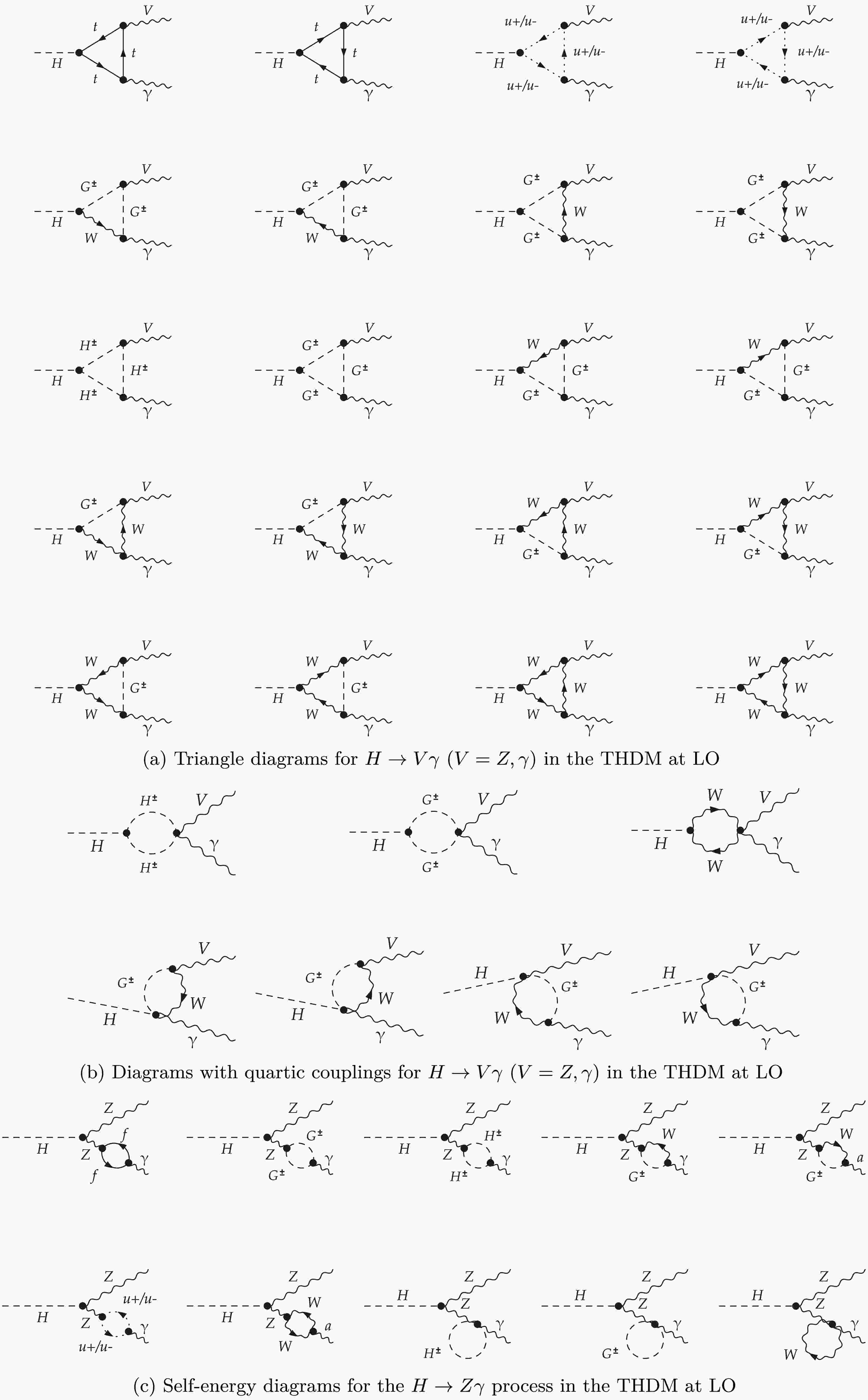
Note that the $ H\to\gamma\gamma $ width includes the statistical factor of $ 1/2 $ for identical final-state photons.

Both processes are loop-induced. The corresponding LO Feynman diagrams are shown in Figure 1. At LO, 31 and 50 Feynman diagrams contribute to the $ H \to \gamma\gamma $ and $ H \to Z\gamma $ processes, respectively. The topologies common to both processes are displayed in Figures 1a and 1b. The self-energy diagrams arise exclusively in the $ H\to Z\gamma $ channel, as illustrated in Fig. 1c. These diagrams contribute only to $ A_2 $ and $ A_5 $ and serve to cancel ultraviolet divergences. In practice, if Eq. (14) is applied first and only the form factor $ A_4 $ is retained, the self-energy diagrams can be discarded directly. We have explicitly verified the Ward identity at both LO and NLO. The LO amplitude can be decomposed into three contributions: top-quark loops, the W-boson sector (diagrams involving the W boson, ghosts, or Goldstone bosons), and charged-Higgs loops. These combine as

Figure 1.  Feynman diagrams for the $ H \to V\gamma $ $ (V=Z,\gamma) $ process in the THDM at LO

The corresponding LO expressions are presented in Appendix A, and the relevant THDM couplings for both processes are summarised in Table II.

The NLO QCD Feynman diagrams are shown in Figure 2. The calculation involves 24 two-loop diagrams, together with the corresponding counterterm diagrams. The counterterm diagrams include the Z–γ mixing contribution relevant to the $ H\to Z\gamma $ channel. In the on-shell (OS) renormalisation scheme, the following identity holds for an on-shell external photon: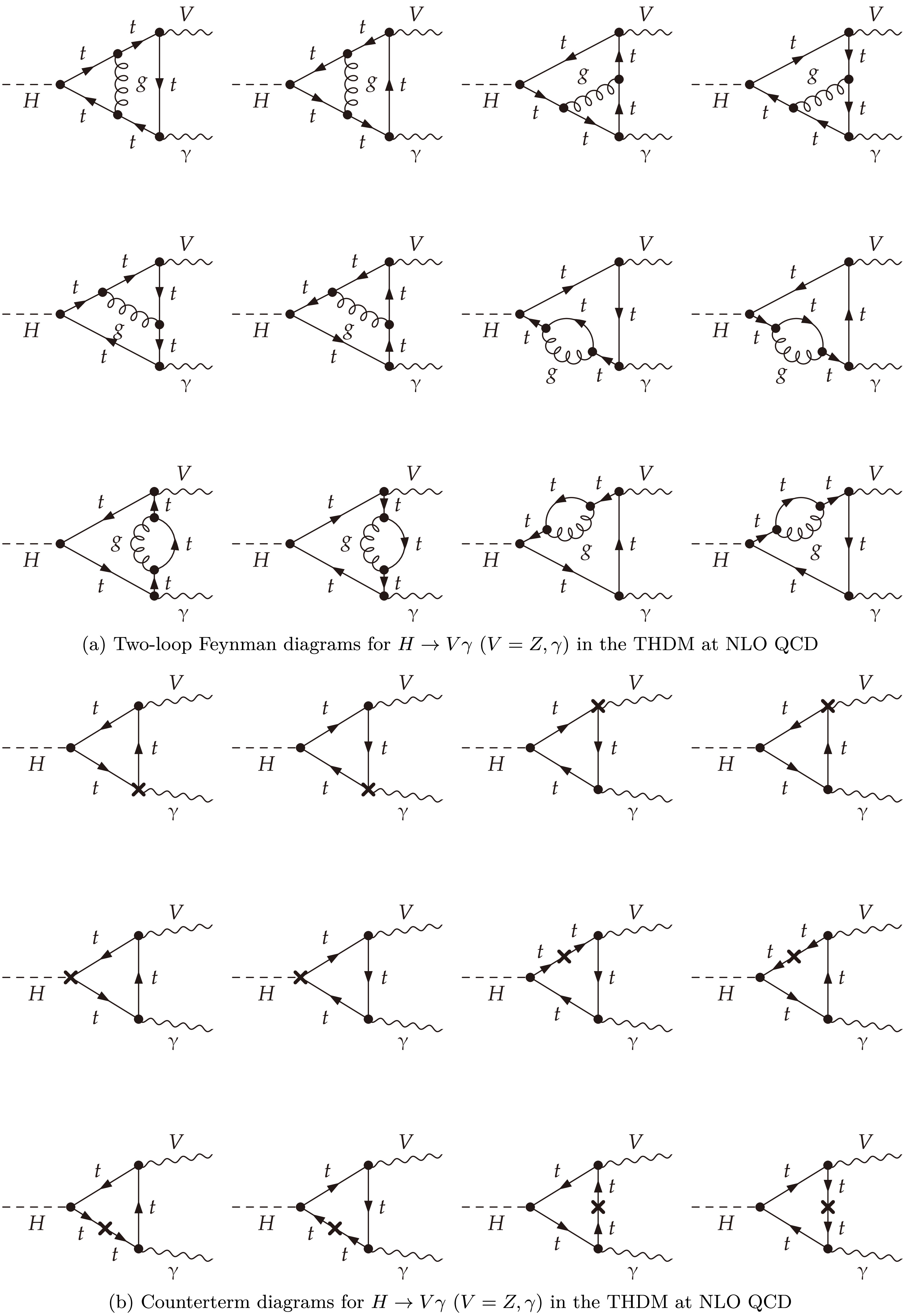

Figure 2.  Feynman diagrams for $ H \to V\gamma $ $ (V=Z,\gamma) $ in the THDM at NLO QCD

(18)

The rightmost diagram corresponds to the self-energy diagram shown in Fig. 1c. This identity can be readily established by explicitly writing out the relevant amplitudes. The contribution from the $ HZ\gamma $ vertex counterterm (first diagram) is

while the Z–γ mixing counterterm insertion (second diagram) is given by

Thus, the first two diagrams cancel exactly, and only the renormalised Z–γ mixing self-energy insertion on the external photon leg remains. This cancellation, which ensures that no net $ H\to ZZ $ contribution enters the $ H\to Z\gamma $ amplitude through the mixing counterterm, is the standard treatment adopted in previous $ HZ\gamma $ calculations [37, 72, 73]. Moreover, at NLO QCD, the unrenormalised Z–γ mixing self-energy vanishes for an on-shell external photon, $ {\Sigma}_{Z\gamma}(0)=0 $ [74], so no additional mixing contribution is required at this order. Because all fermion Yukawa couplings in the Type-I THDM scale as $ \cot\beta $, the bottom-quark loop is suppressed relative to the top-quark loop by $ (m_b/m_t)^2\approx 5\times 10^{-4} $ and can therefore be neglected.

The top-quark wave-function renormalisation constant $ \delta Z_f $ does not appear explicitly in the final physical amplitude, because its contributions cancel in the sum of all counterterm diagrams. For a fermion field, the bare and renormalised fields are related by

so that the fermion propagator counterterm reads

　　　　　　　　(22)

Inserting this counterterm into the fermion propagator yields

(23)

For the $ Sf\bar{f} $ and $ Vf\bar{f} $ vertices, similar contributions from fermion-field renormalisation enter the vertex counterterms. Summing over all counterterm diagrams, the contributions from $ \delta Z_f $ cancel exactly, leaving no net effect on the physical NLO amplitude. The only renormalisation constant required is the quark-mass counterterm, which in the OS scheme takes the form [75]

where μ is the renormalisation scale, $ C_F = 4/3 $, and $ d = 4 - 2\epsilon $ is the spacetime dimension.

In this work, the one-loop form factors are denoted by $ A_i^{\text{(1-loop)}} $, whereas the two-loop contributions at $ {\cal{O}}(\alpha_s) $ are denoted by $ A_i^{\text{(2-loop)}} $. At LO, the squared amplitude reduces to

At NLO, the squared amplitude is expanded to $ {\cal{O}}(\alpha_s) $, yielding

The decay width at each perturbative order is obtained by substituting the corresponding squared amplitude into Eq. (16).

To quantify the impact of QCD corrections beyond LO, we introduce the relative correction, defined as

where $ \Delta_{\mathrm{QCD}}=\Gamma_{\mathrm{NLO}} - \Gamma_{\mathrm{LO}} $.

The Feynman diagrams and corresponding amplitudes are generated using the Mathematica package FeynArts 3.11 [76] and are subsequently simplified with FeynCalc 10.0.0 [77−80]. All calculations are carried out in the 't Hooft–Feynman gauge. At LO, the one-loop integrals are decomposed into Passarino–Veltman functions and numerically evaluated with Package-X [81, 82]. The NLO QCD corrections involve a substantial number of two-loop scalar integrals. The integration-by-parts (IBP) reduction is performed with Kira 2.3 [83, 84]. The resulting master integrals (MIs) are computed using the auxiliary mass flow (AMF) method [85−87], which provides an efficient numerical framework based on differential equations with systematically determined boundary conditions. In practice, we use the package AMFlow [88], which implements the AMF method, to obtain high-precision numerical results for all MIs. Finally, the one-loop results have been cross-checked against those from the program H-COUP 3.0, thereby validating the correctness of our implementation.

The SM input parameters are taken as follows [52]:

The strong coupling constant $ \alpha_s(\mu) $ is evolved from $ \mu = m_Z $ to the relevant energy scale $ \mu = \sqrt{s} $ using the $ \mathrm{RunDec}$ package [89, 90].

The parameter space is scanned over the following ranges:

We first consider the alignment limit, i.e., $ s_{\beta-\alpha}=1 $. A sample of 5000 parameter points that satisfy all theoretical and experimental constraints detailed in Sec. II is retained.

In Figure 3, the LO decay widths for the two processes are projected onto various parameter planes. The results for $ H \to \gamma\gamma $ and $ H \to Z\gamma $ are shown in the left and right panels, respectively. The viable points cluster predominantly at small values of $ \tan\beta $, with $ M^2 $ approximately proportional to $ m_H^2 $; this feature is driven primarily by theoretical constraints. The irregular structure in the region $ m_H \sim 200 $–$ 400\; \mathrm{GeV} $ originates from experimental constraints on $ H^+ \to q q^{\prime} $ [91, 92] and $ \phi \to \gamma\gamma / \tau\tau $ [93, 94], consistent with the behaviour reported in Ref. [58]. The decay widths of both processes exhibit similar patterns across the projected planes. As the neutral Higgs mass increases, the decay widths tend to grow owing to the enlarged phase space. Overall, the decay width for $ H \to \gamma\gamma $ systematically exceeds that for $ H \to Z\gamma $. For $ m_H \lesssim 400\; \mathrm{GeV} $ and $ M^2 \lt 8\times10^4\; \mathrm{GeV}^2 $, the decay widths for both processes are strongly suppressed, falling below approximately $ 1\times10^{-5} $ and $ 3\times10^{-6} $ for $ H \to \gamma\gamma $ and $ H \to Z\gamma $, respectively.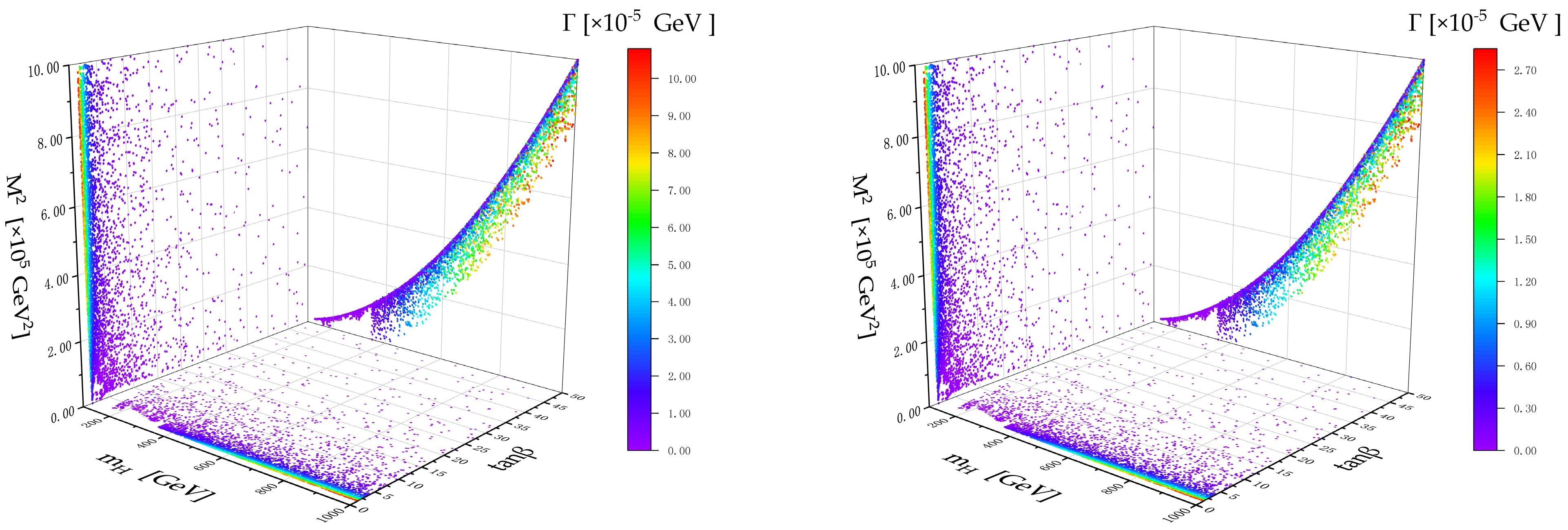

Figure 3.  Leading-order decay widths for $ H \to \gamma\gamma $ (left panel) and $ H \to Z\gamma $ (right panel), projected onto different parameter planes for the 5000 viable parameter points in the alignment limit ($ s_{\beta-\alpha}=1 $).

As also shown in Figure 3, the decay widths decrease rapidly with increasing $ \tan\beta $. This decrease is monotonic and admits a simple explanation. In the alignment limit ($ c_{\beta-\alpha}=0 $), the $ HWW $ coupling vanishes, implying $ A_W^{(1\text{-}\mathrm{loop})}=0 $. The LO decay width therefore receives contributions only from the top-quark loop, the charged-Higgs loop, and their interference,

From Eqs. (A5) and (A6), the scalar loop function $ {\cal{A}}_0 $ is of the same order as the fermionic one, $ {\cal{A}}_{1/2} $. In the alignment limit, however, Eq. (A2) shows that the charged-Higgs contribution is further suppressed by the effective trilinear coupling

which remains small over most of the viable parameter space. As a result, unless $ \tan\beta $ becomes very large, both the pure charged-Higgs contribution and the interference term are numerically negligible compared with the top-quark loop. The total decay width is therefore well approximated by

which naturally explains the observed monotonic decrease with increasing $ \tan\beta $. Figure 4 illustrates how each contribution scales with $ \tan\beta $: $ \Gamma_{\mathrm{top}} $ exceeds both $ \Gamma_{H^\pm} $ and $ \Gamma_{t\text{-}H^\pm} $ by several orders of magnitude over nearly the entire $ \tan\beta $ range. Because the viable THDM parameter space is concentrated at moderate $ \tan\beta $, this $ \cot^2\beta $ scaling governs the decay widths throughout the phenomenologically relevant region.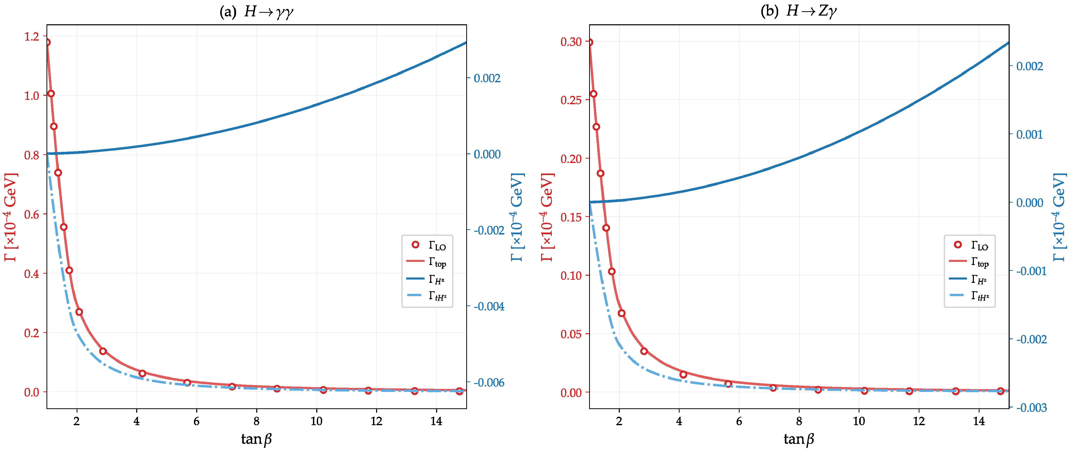

Figure 4.  Decomposition of the LO decay width into top-quark ($ \Gamma_{\mathrm{top}} $, red solid line), charged-Higgs ($ \Gamma_{H^\pm} $, blue solid line), and interference ($ \Gamma_{t\text{-}H^\pm} $, blue dashed line) contributions in the alignment limit ($ s_{\beta-\alpha}=1 $), for $ m_H=489 $ GeV and $ M^2=226674 $ GeV$ ^2 $. The red curves should be read using the left axis, and the blue curves using the right axis. The red circles indicate the total LO width $ \Gamma_{\mathrm{LO}} $. Panel (a): $ H\to\gamma\gamma $; panel (b): $ H\to Z\gamma $.

The relative corrections for the two processes are presented in Figure 5. Results for $ H \to \gamma\gamma $ appear in the left panels, and those for $ H \to Z\gamma $ in the right panels. The relative corrections exhibit no appreciable dependence on $ \tan\beta $ and depend primarily on $ m_H $. On both the $ m_H $–$ \tan\beta $ and $ m_H $–$ M^2 $ planes, distinct colour-coded bands corresponding to different values of $ m_H $ are clearly visible. As $ m_H $ increases, the relative correction first rises and then falls, attaining its maximum in the vicinity of the $ t\bar{t} $ production threshold. Beyond this threshold, the relative correction decreases monotonically and eventually changes sign from positive to negative. At $ m_H \sim 1000\; \mathrm{GeV} $, the relative correction is approximately $ -20$%. At very small values of $ m_H $ or $ M^2 $, a few isolated outliers appear, where the relative corrections become appreciably large. This behaviour is attributable to the strong suppression of the LO decay width in these regions, while the NLO contribution retains a moderate magnitude, as shown in Figure 3 and Figure 6.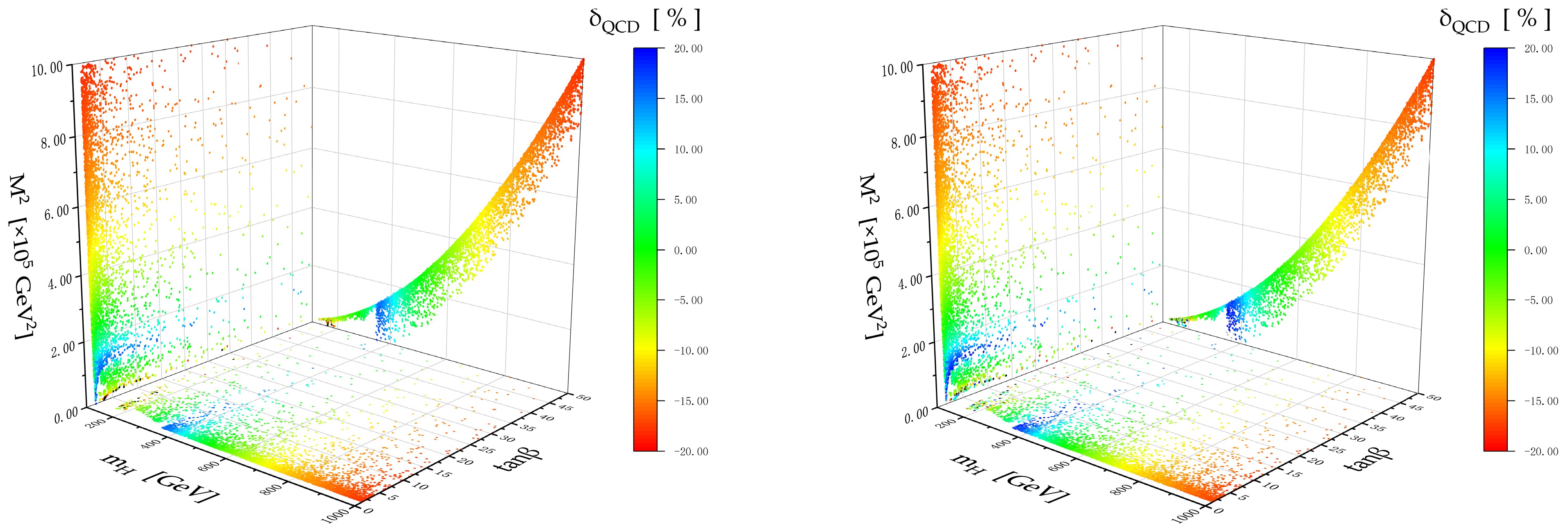

Figure 5.  Relative corrections $ \delta_{\mathrm{QCD}} $ for $ H \to \gamma\gamma $ (left panel) and $ H \to Z\gamma $ (right panel) at NLO, projected onto different parameter planes.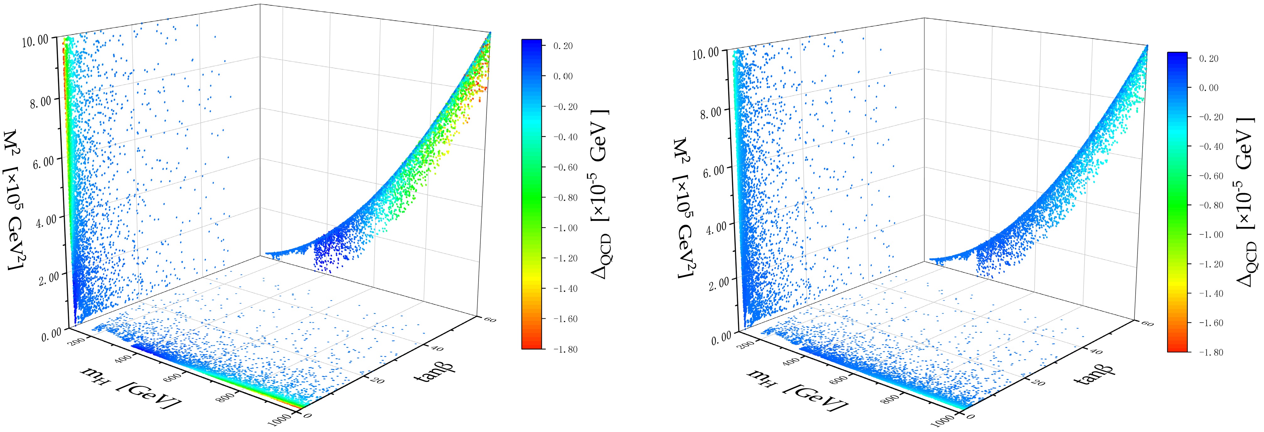

Figure 6.  Absolute corrections, $ \Delta_{\mathrm{QCD}} $, for $ H \to \gamma\gamma $ (left panel) and $ H \to Z\gamma $ (right panel) at NLO, projected onto different parameter planes for the same parameter sample as in Figure 3.

Figure 6 displays the NLO contributions $ \Delta_{\text{QCD}} $. The parametric dependence of the NLO contributions mirrors that observed at LO. The NLO corrections arise from the top-quark loop, whose Yukawa coupling scales as $ \cot\beta $. Consequently, the interference between the two-loop and one-loop amplitudes reproduces the LO pattern.

To illustrate the individual parameter dependences more transparently, one-dimensional projections are presented below. Figure 7 displays the decay widths and corresponding NLO QCD relative corrections as functions of $ \tan\beta $ for $ H \to \gamma\gamma $ (left panel) and $ H \to Z\gamma $ (right panel), with $ M^2 = m_H^2 $. In each panel, three curves are shown, corresponding to $ s_{\beta-\alpha} = 0.98,\, 0.99, $ and $ 1 $. Results are presented for $ m_H = 350,\, 550, $ and $ 850\; \mathrm{GeV} $, thereby facilitating a direct comparison of the mass dependence across different $ m_H $ values.

Figure 7.  Decay widths and relative corrections for $ H \to \gamma\gamma $ (left) and $ H \to Z\gamma $ (right) as functions of $ \tan\beta $ for different values of $ m_H $ and $ s_{\beta-\alpha} $, with $ M^2=m_H^2 $. From top to bottom: $ m_H=350 $, $ 550 $, and $ 850\; \mathrm{GeV} $. In each panel, the upper plot shows the LO and NLO decay widths for $ s_{\beta-\alpha}=0.98 $, $ 0.99 $, and 1, and the lower plot shows the corresponding relative correction $ \delta_{\mathrm{QCD}} $.

In both channels, the decay widths decrease monotonically with increasing $ \tan\beta $. In the $ H \to \gamma\gamma $ channel, the three $ s_{\beta-\alpha} $ curves are most widely separated at $ m_H = 350\; \mathrm{GeV} $. As $ m_H $ increases, the differences between the curves progressively diminish, and by $ m_H = 550\; \mathrm{GeV} $ the decay-width curves nearly converge. In contrast, in the $ H \to Z\gamma $ channel, the three curves remain discernibly separated over the full $ m_H $ range, although the spacing between them decreases as $ m_H $ increases. In general, the decay width is enhanced for smaller $ s_{\beta-\alpha} $, because the $ HWW $ coupling is proportional to $ c_{\beta-\alpha} $ and the magnitude of $ \kappa_{f,H} $ increases as $ s_{\beta-\alpha} $ decreases, as shown in Table II. For $ m_H = 350\; \mathrm{GeV} $, the corrections with $ s_{\beta-\alpha}\neq 1 $ decrease monotonically with increasing $ \tan\beta $, crossing zero at $ \tan\beta\approx 5 $ ($ s_{\beta-\alpha}=0.98 $) and $ \tan\beta\approx 7 $ ($ s_{\beta-\alpha}=0.99 $); by contrast, the $ s_{\beta-\alpha}=1 $ curve remains flat, since the $ \cot^2 \beta $ scaling cancels exactly in the ratio $ \delta_{\mathrm{QCD}} $. At $ m_H = 550\; \mathrm{GeV} $, the $ s_{\beta-\alpha}\neq 1 $ curves become mildly non-monotonic. In the $ H\to\gamma\gamma $ channel, they begin slightly negative at small $ \tan\beta $, rise to a shallow positive maximum of about $ 0.6$% near $ \tan\beta\approx 3 $–$ 5 $, and then decrease to progressively more negative values. In the $ H\to Z\gamma $ channel, they start positive (around $ 3$%), peak near $ \tan\beta\approx 1 $–$ 2 $, and subsequently decrease, eventually becoming negative at large $ \tan\beta $. By contrast, at $ m_H = 850\; \mathrm{GeV} $, the corrections with $ s_{\beta-\alpha}\neq 1 $ increase monotonically with $ \tan\beta $ in both channels, reaching about $ +38$% for $ s_{\beta-\alpha}=0.98 $ in the $ H\to\gamma\gamma $ channel at large $ \tan\beta $. In the $ H\to Z\gamma $ channel, these curves likewise cross zero and become positive, attaining roughly $ +2$% for $ s_{\beta-\alpha}=0.98 $.

The QCD corrections to the amplitude originate solely from top-quark loops. A top-only analysis therefore already captures the essential features, in particular the neutral-Higgs mass dependence shown in Figure 3. We accordingly define the decoupling limit as the regime in which only the top-quark loop contributes, corresponding to $ s_{\beta-\alpha}=1 $ together with $ m_{H}^2=M^2 $.

In Figure 8, we depict the decay widths and relative QCD corrections for the $ H \to \gamma\gamma $ and $ H \to Z\gamma $ channels in this case, choosing $ \tan\beta = 1.5 $, as functions of the heavy Higgs mass $ m_H $. Within the $ m_H $ range considered, the decay widths and relative corrections for both channels exhibit closely analogous behaviour. The decay widths increase with $ m_H $. Quantitatively, the $ H \to \gamma\gamma $ decay width exceeds that of $ H \to Z\gamma $ by approximately a factor of four. The relative QCD corrections range from $ -20$% to $ +20$%, following nearly identical trends in the two channels. A pronounced peak is evident near the $ t\bar{t} $ production threshold, where the corrections reach approximately $ 15$%. Beyond this threshold, the QCD corrections become negative and continue to decrease with increasing $ m_H $.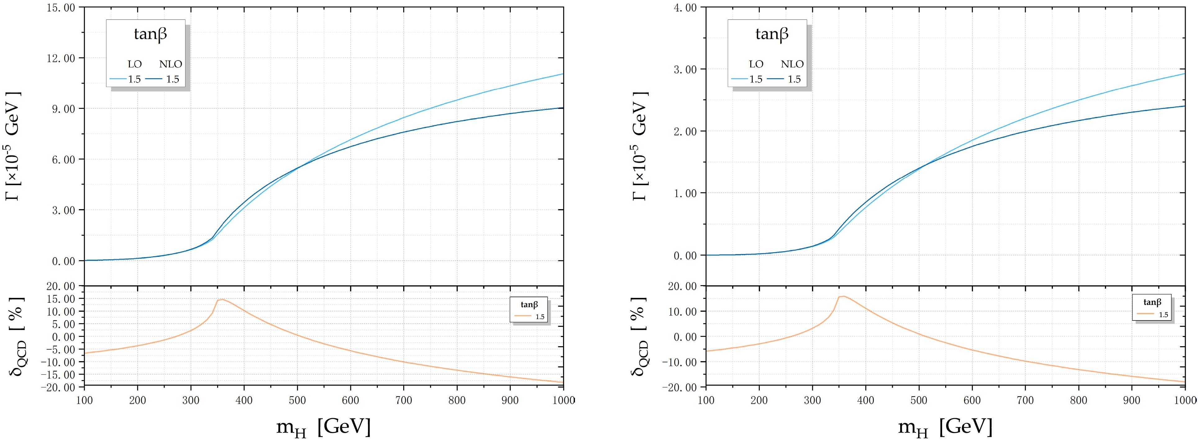

Figure 8.  Decay widths and relative corrections for $ H \to \gamma\gamma $ (left) and $ H \to Z\gamma $ (right) as functions of $ m_H $ for $ \tan\beta = 1.5 $, in the decoupling limit ($ s_{\beta-\alpha}=1 $ and $ M^2=m_H^2 $). In each panel, the upper plot shows the decay widths at LO and NLO, and the lower plot shows the relative correction $ \delta_{\mathrm{QCD}} $.

The pronounced enhancement near the $ t\bar t $ threshold in Fig. 8 prompts the question of whether the fixed-order QCD prediction remains reliable in that region. Unlike processes dominated by an S-wave heavy-quark pair, the threshold behaviour of the scalar Higgs decay amplitudes is governed by a P-wave configuration, for which Coulomb effects are strongly suppressed [95]. This suppression follows directly from the quantum numbers of the intermediate $ t\bar t $ state.

For a $ CP $-even Higgs boson, the Yukawa interaction $ y_t\bar t tH $ conserves $ CP $, requiring the intermediate $ t\bar t $ pair to have quantum numbers

The lowest S-wave configuration, $ {}^{1}S_{0} $, instead carries

and is therefore forbidden by $ CP $ conservation. Consequently, the lowest allowed threshold state is the $ {}^{3}P_{0} $ configuration, implying that the production amplitude is proportional to the relative momentum of the heavy quarks.

Near threshold, multiple Coulomb-gluon exchanges are conventionally resummed into the Sommerfeld factor [95−97],

where

and $ \beta_t=\sqrt{1-4m_t^2/m_H^2} $ denotes the top-quark velocity. Since the real part of the amplitude can be reconstructed from its imaginary part through a dispersion relation, the threshold behavior is most transparently understood by first examining the imaginary part.

Taking $ H\to\gamma\gamma $ as an example, the amplitude reads

where $ {\cal{A}}_{1/2}^{\text{(2-loop)}} $ is taken from Refs. [16, 30], and the full expression is given in Eq. (A8) of Appendix A. The one-loop form factor admits the threshold expansion

which immediately gives

As shown in Ref. [95], the Coulomb correction factor $ C_{\text{Coul}} $ modifies the imaginary part of a P-wave amplitude only through terms that vanish at threshold, whereas the corresponding correction to an S-wave process approaches a finite constant owing to the familiar Sommerfeld enhancement. Eq. (35) then implies a $ \beta_t^2 $ suppression of the Coulomb-corrected imaginary part. Through the dispersion relation, the real part likewise receives only finite corrections and varies smoothly across the threshold, in contrast to the logarithmic singularity characteristic of an S-wave amplitude. Consequently, the Coulomb effect produces only a negligible modification to the threshold behavior of the present processes. These features already suggest that the fixed-order prediction remains well behaved across the threshold.

We now explicitly expand the result near threshold at $ {\cal{O}}(\alpha_s) $. For the $ H\to\gamma\gamma $ amplitude, the threshold expansion of the two-loop form factor is

where the threshold constant is

$ \widetilde{c}_2 = -8 + \dfrac{9}{2}\pi^2 - 7\pi^2\ln 2 $ is a real constant, and Θ denotes the Heaviside step function. Compared with the LO expansion in Eq. (38), this result shows that the leading contribution to the real part remains finite at threshold, while the first non-analytic correction is proportional to $ \beta_t^2\ln\beta_t $. Meanwhile, the imaginary part is given by

which is consistent with Eq. (35). Therefore, the two-loop QCD correction preserves the same qualitative threshold structure already present at leading order: no Coulomb singularity develops, and the enhancement observed in Fig. 8 should be interpreted as a genuine perturbative threshold effect rather than as a manifestation of the breakdown of fixed-order perturbation theory. Moreover, the relative correction at the threshold is

which is approximately $ 1.22\alpha_s $, indicating well-behaved perturbative convergence near the threshold.

Strictly speaking, in the asymptotic threshold region where $ \beta_t\sim\alpha_s $, higher-order non-relativistic effects can still be incorporated systematically through threshold resummation. However, owing to the absence of Sommerfeld enhancement in the $ {}^{3}P_{0} $ channel, these contributions provide only finite quantitative modifications and do not alter the analytic structure established above. We therefore expect the fixed-order calculation presented here to provide a reliable description of the overall magnitude, sign, and threshold behaviour of the QCD corrections, although the detailed line shape in an extremely narrow region around $ m_H\simeq2m_t $ may receive moderate higher-order refinements.

To assess the residual perturbative uncertainty of the NLO predictions presented above, we vary the renormalisation scale over the range $ \mu\in[m_H/2,\,2m_H] $. In our calculation, the strong coupling constant is renormalised in the $ \overline{\mathrm{MS}} $ scheme, while the quark mass is renormalised on shell, so that the μ dependence at NLO enters only through the coupling,

with $ \Delta=\Delta_{\mathrm{QCD}}/\alpha_s(\mu) $ and $ \Gamma_{\mathrm{LO}} $ independent of μ. We define the scale-variation uncertainty as

and, using the one-loop running $ \alpha_s(k\mu)\simeq\alpha_s(\mu)- \beta_0\,\alpha_s^2(\mu)\ln k $ with $ \beta_0=(33-2n_f)/(6\pi) $, one obtains $ R(\mu)\simeq 2\beta_0\,\alpha_s(\mu)\ln 2\simeq 1.69\,\alpha_s(\mu) $ for $ n_f=5 $. In the range $ 126\; \mathrm{GeV}<\mu<1000\; \mathrm{GeV} $, $ \alpha_s(\mu)\simeq 0.09 $–$ 0.11 $, which gives $ R(\mu)\simeq 0.15 $–$ 0.19 $. Since the relative corrections satisfy $ |\delta_{\mathrm{QCD}}|\lesssim 20$% over the viable parameter space, the resulting perturbative uncertainty is bounded by $ \varepsilon\simeq 0 $–$ 3.8$%. The factor $ 1/(1+\delta_{\mathrm{QCD}}) $ does enhance ε for negative corrections. However, these occur only at large $ m_H $, where $ \alpha_s(\mu) $ (and hence $ R(\mu) $) is smallest, so the bound still holds. Representative values in the decoupling limit ($ s_{\beta-\alpha}=1 $, $ M^2=m_H^2 $) are collected in Table III. The largest uncertainty, $ \varepsilon=3.1$% at $ m_H=1000\; \mathrm{GeV} $, lies safely within this estimate, and the $ m_H $ dependence of the tabulated values follows that of $ \delta_{\mathrm{QCD}} $ shown in Figure 8, confirming that the NLO corrections are perturbatively stable over the full mass range considered.

To investigate the phenomenological implications of the NLO QCD corrections, we evaluate $ \sigma(gg\to H)\times \mathrm{Br}(H\to V\gamma) $ for both the $ \gamma\gamma $ and $ Z\gamma $ final states and compare the results with the existing ATLAS upper limits at $ \sqrt{s}=13 $ TeV. The gluon-fusion production cross section is evaluated as $ \sigma(gg\to H) = \sigma_{\mathrm{SM}}^{\mathrm{NNLO+NNLL}}(m_H)\times\cot^{2}\beta $, where $ \sigma_{\mathrm{SM}}^{\mathrm{NNLO+NNLL}}(m_H) $ denotes the SM Higgs boson production cross section at NNLO+NNLL accuracy, as tabulated by the LHC Higgs Cross Section Working Group [98]. In the alignment limit of the Type-I THDM, every fermion coupling to H scales as $ \kappa_{f,H}=-\cot\beta $; hence, $ \kappa_{t,H}^{2}=\cot^{2}\beta $, and the rescaling is exact at the amplitude level. The branching ratios are computed as $ \mathrm{Br}(H\to V\gamma)= \Gamma(H\to V\gamma)/\Gamma_{\mathrm{total}}(H) $, where the numerator is evaluated at LO and NLO as described in Sec. III, and $ \Gamma_{\mathrm{total}}(H) $ is the total decay width of H obtained using $ \mathrm{H-COUP}$ 3.0. The same $ \sigma(gg\to H) $ and $ \Gamma_{\mathrm{total}}(H) $ are used for both the LO and NLO predictions, so that the difference arises solely from the NLO QCD correction to $ \Gamma(H\to V\gamma) $.

The results are presented in Fig. 9. In the $ H\to\gamma\gamma $ channel [panel (a)], the predictions are compared with the ATLAS diphoton search based on 139 fb$ ^{-1} $ [7]. The experimental limits are reported as fiducial cross sections; accordingly, the theoretical predictions are multiplied by the acceptance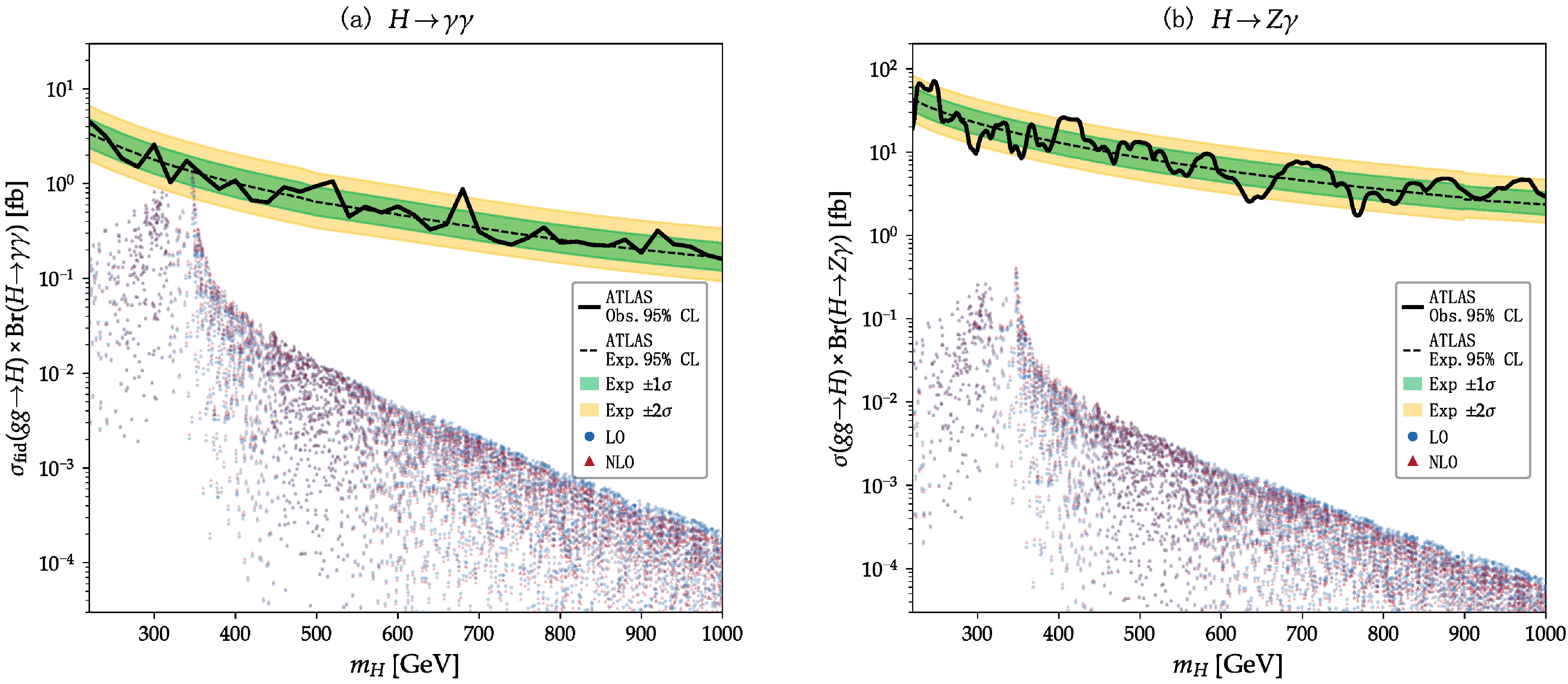

Figure 9.  Predictions for $ \sigma(gg\to H)\times\mathrm{Br}(H\to V\gamma) $ at LO and NLO QCD, compared with the ATLAS 95% CL upper limits for $ H\to\gamma\gamma $ (a) and $ H\to Z\gamma $ (b). The blue circles and red triangles denote the LO and NLO predictions for the 5000 viable parameter points, respectively. The solid and dashed black curves indicate the observed and expected limits, while the green and yellow bands represent the $ \pm1\sigma $ and $ \pm2\sigma $ ranges of the expected limit.

parametrised in the same reference. The NLO fiducial prediction reaches about 1.30 fb at $ m_H\approx 347 $ GeV, which is roughly 83% of the observed ATLAS limit of 1.56 fb, compared with 1.13 fb (73%) at LO. The $ \sim +15$% NLO correction therefore reduces the gap from 0.43 fb to 0.26 fb. In the $ H\to Z\gamma $ channel [panel (b)], the predictions are compared with the ATLAS search based on 140 fb⁻¹ [99]. The maximum $ \sigma\times\mathrm{Br} $ at NLO is approximately 0.41 fb near the $ t\bar{t} $ threshold ($ m_H\approx 347 $ GeV), which is about 30 times below the observed ATLAS limit of approximately 12 fb. Thus, the $ Z\gamma $ channel does not yet constrain the alignment-limit parameter space. With the anticipated luminosity increase at the HL-LHC, the $ {\cal{O}} $(15%) NLO corrections may alter the exclusion boundary in the $ (m_{H},\,\tan\beta) $ plane.

In this work, we have investigated the decays of the heavy neutral $ CP $-even Higgs boson into diphoton and $ Z\gamma $ final states within the framework of the Type-I THDM. A complete numerical evaluation has been carried out while retaining the full quark-mass dependence. Working in the alignment limit, we imposed the phenomenological constraints and evaluated the decay widths of both processes at NLO QCD accuracy for all viable parameter points. To elucidate the dependence on individual parameters, one-dimensional projections were also presented. Our findings indicate that the $ H \to \gamma\gamma $ decay width typically exceeds that of $ H \to Z\gamma $ by approximately a factor of four. The decay widths grow monotonically with $ m_H $ owing to the enlarged phase space, while decreasing with increasing $ \tan\beta $, since the dominant top-quark contribution to the width scales as $ \cot^2\beta $. The LO amplitude is dominated by the top-quark loop, with the W-boson contribution vanishing in the alignment limit and the charged-Higgs contribution suppressed across most of the viable parameter space. The QCD corrections span approximately from $ -20$% to $ +20$%, depending on the parameter configuration. The relative corrections exhibit a pronounced peak in the vicinity of the $ t\bar{t} $ production threshold and become negative for heavier Higgs-boson masses. Away from the alignment limit, the relative corrections in the $ H \to \gamma\gamma $ channel can reach values as large as $ +38$% at elevated $ \tan\beta $, while in the $ H\to Z\gamma $ channel the corrections for $ s_{\beta-\alpha}\neq 1 $ likewise cross zero and become positive. Analytic expressions for the one-loop amplitudes in the alignment limit have been provided, with $ H\to\gamma\gamma $ taken as an example. Owing to $ CP $ conservation, the intermediate $ t\bar t $ pair is produced in the $ {}^{3}P_{0} $ state, for which Coulomb effects are strongly suppressed and the threshold behaviour remains perturbative. The threshold expansion of the complete two-loop amplitude confirms that the QCD correction remains finite, with an imaginary part proportional to $ \beta_t^2 $ and a finite real part at threshold, in agreement with the expected P-wave behaviour. These results demonstrate that the fixed-order prediction provides a stable description of both the overall size and the threshold behaviour of the QCD corrections for the two processes, while any higher-order threshold effects are expected to induce only finite quantitative modifications. The residual perturbative uncertainty, estimated by varying the renormalisation scale over $ \mu\in[m_H/2,\,2m_H] $, is bounded by approximately $ 3.8$% across the viable parameter space, well below the typical size of the corrections themselves. A phenomenological analysis comparing $ \sigma(gg\to H)\times\mathrm{Br}(H\to V\gamma) $ with the ATLAS 95% CL upper limits reveals that the $ H\to\gamma\gamma $ predictions at NLO already reach approximately 83% of the observed limit near the $ t\bar{t} $ threshold, whereas the $ H\to Z\gamma $ channel remains roughly 30 times below the current sensitivity. Should the experimental sensitivity approach the current exclusion limit with the increased luminosity at the HL-LHC, the $ {\cal{O}} $(15%) NLO corrections may become relevant for interpreting the exclusion boundary in the $ (m_H,\,\tan\beta) $ plane. These results provide a comprehensive characterisation of the loop-induced decay properties of the heavy neutral Higgs boson in the Type-I THDM and may serve as valuable input for forthcoming experimental searches and precision measurements at hadron colliders.

In this appendix, we collect the analytic expressions entering the calculation of $ H\to V\gamma $ ($ V=Z,\gamma $) within the Type-I THDM. The kinematic variables are

The complete one-loop amplitude for $ H\to V\gamma $ can be written in the compact form

where the coefficients are

and the effective trilinear Higgs–charged-Higgs coupling is

The scalar form factors for spin-$ \tfrac12 $, spin-$ 0 $, and spin-$ 1 $ intermediate states can be expressed in terms of the two basic integrals $ I_1 $ and $ I_2 $ as

The integrals $ I_1 $ and $ I_2 $ are defined as

where the primary functions $ f(\tau) $ and $ g(\tau) $ are

For completeness, we also present the two-loop form factor $ {\cal{A}}_{1/2}^{\text{(2-loop)}} $ for the $ H\to\gamma\gamma $ channel, which corresponds to the $ {\cal{A}}_{1/2}^{\text{(2-loop)}} $ term in Eq. (37):

with

For the $ H\to Z\gamma $ channel, the two-loop form factor involves 28 master integrals that depend on three mass scales and is expressed in terms of logarithms, the polylogarithms $ \mathrm{Li}_n $ ($ n=2,3,4 $), and the two-variable function $ \mathrm{Li}_{2,2} $. We evaluate these master integrals using $ \mathrm{AMFlow}$ and find agreement with Ref. [25]. The full analytic expression is too lengthy to be presented here.