


 Abstract
 HTML
 Reference
 Related
 PDF



-
The ringdown stage of a perturbed black hole (BH) is governed by its quasinormal modes (QNMs), whose complex frequencies determine the oscillation rates and damping times of the spacetime response. QNMs therefore play a central role in BH spectroscopy and provide a direct link between gravitational-wave (GW) observations and the properties of compact objects [1−5]. In the standard description, the ringdown signal is written as a superposition of exponentially damped modes. A fundamental issue, however, is how reliably these modes can be identified and extracted from time-domain waveforms, especially when several modes contribute at comparable levels or when the relevant frequencies are nearly degenerate [6−8].
Previous studies have developed rigorous spectral formulations of QNMs using operator-theoretic methods and hyperboloidal spectral decompositions [9−11]. The non-self-adjoint character of the QNM problem is closely tied to the radiative boundary conditions, namely purely ingoing waves at the horizon and purely outgoing waves at spatial infinity. This connects the QNM spectral problem to the broader framework of non-Hermitian physics [12−14]. As a result, the spectrum can exhibit pronounced sensitivity to perturbations, pseudospectral broadening, resonance, and other effects familiar from non-Hermitian theory [15−23]. Among these, exceptional points (EPs) have attracted increasing attention in BH perturbation theory, especially with the advent of high-precision GW astronomy [24−28]. An EP is a spectral degeneracy at which two eigenvalues and their associated eigenfunctions coalesce [29−37]. Near such a point, the spectrum develops the characteristic square-root branch structure, which is associated with a variety of phenomena, including mode switching, hysteresis, and resonant behavior [38−41].
EPs generally require a parameter space with dimension greater than one. A representative example is provided by massive scalar perturbations of Kerr BHs, where EPs appear in the parameter space spanned by the BH spin and the scalar mass [39, 42−45]. A related construction can also be realized by adding a Gaussian bump to the curvature effective potential that governs BH perturbations, and this idea has recently been extended from isolated EPs to continuous exceptional lines [40, 46, 47]. By contrast, when only a restricted one-parameter scan is available, an exact EP is generically replaced by mode repulsion or an avoided crossing, which can be understood as the one-dimensional trace of a nearby EP in a higher-dimensional parameter space [38, 48−55].
These features are important not only for organizing the QNM spectrum in the frequency domain, but also for describing ringdown signals in the time domain. Near an EP, the usual expansion in terms of independent exponentially damped QNMs is modified by a resonant contribution containing both an exponential factor and a term linear in time [40]. Consequently, the presence of an EP can leave a characteristic imprint on the waveform and affect the extraction and interpretation of ringdown signals. Recent studies have also indicated that an EP-based description can capture near-resonant BH ringdown more naturally than the standard superposition of independent damped modes [41, 56].
Most existing studies of EPs in BH perturbation theory have focused on BHs satisfying the no-hair theorem, whereas the corresponding problem in hairy BH backgrounds remains much less explored. This naturally raises the question of whether similar non-Hermitian structures also arise in BH solutions with nontrivial hair. In particular, hairy BHs in the Einstein-Maxwell-scalar (EMS) theory provide a useful setting in which to investigate this issue. The theory admits asymptotically flat BH solutions with scalar hair and contains two independent control parameters, allowing for a richer spectral structure [57−68]. More importantly, recent studies of the scalar QNM spectrum of EMS hairy BHs have identified two distinct families of modes with different spectral stability properties: peak modes, which are localized near the potential peak and are associated with the photon sphere, and off-peak modes, which are localized away from the potential peak and retain an imprint of the valley structure arising in the double-peaked effective potential [69]. An avoided crossing between a peak-mode branch and an off-peak-mode branch was also observed, suggesting that an EP may emerge once the full two-parameter space is explored.
In this paper, we study EPs in the scalar QNM spectrum of hairy BHs in the EMS model and investigate their implications for ringdown signals. Specifically, we identify an EP in the QNM spectrum and compare the corresponding time-domain extraction using the standard QNM ansatz and an EP-based ansatz. The remainder of this paper is organized as follows. In Sec. II, we briefly review the background hairy BH solutions and the numerical framework. In Sec. III, we present the QNM spectrum and discuss the EP structure. In Sec. IV, we analyze the corresponding ringdown signal and its extraction. We conclude in Sec. V with a summary and discussion. Throughout this work, we employ geometrized units with
$ G=c=1 $ . -
The ringdown stage of a perturbed black hole (BH) is governed by its quasinormal modes (QNMs), whose complex frequencies determine the oscillation rates and damping times of the spacetime response. QNMs therefore play a central role in BH spectroscopy and provide a direct link between gravitational-wave (GW) observations and the properties of compact objects [1−5]. In the standard description, the ringdown signal is written as a superposition of exponentially damped modes. A fundamental issue, however, is how reliably these modes can be identified and extracted from time-domain waveforms, especially when several modes contribute at comparable levels or when the relevant frequencies are nearly degenerate [6−8].
Previous studies have developed rigorous spectral formulations of QNMs using operator-theoretic methods and hyperboloidal spectral decompositions [9−11]. The non-self-adjoint character of the QNM problem is closely tied to the radiative boundary conditions, namely purely ingoing waves at the horizon and purely outgoing waves at spatial infinity. This connects the QNM spectral problem to the broader framework of non-Hermitian physics [12−14]. As a result, the spectrum can exhibit pronounced sensitivity to perturbations, pseudospectral broadening, resonance, and other effects familiar from non-Hermitian theory [15−23]. Among these, exceptional points (EPs) have attracted increasing attention in BH perturbation theory, especially with the advent of high-precision GW astronomy [24−28]. An EP is a spectral degeneracy at which two eigenvalues and their associated eigenfunctions coalesce [29−37]. Near such a point, the spectrum develops the characteristic square-root branch structure, which is associated with a variety of phenomena, including mode switching, hysteresis, and resonant behavior [38−41].
EPs generally require a parameter space with dimension greater than one. A representative example is provided by massive scalar perturbations of Kerr BHs, where EPs appear in the parameter space spanned by the BH spin and the scalar mass [39, 42−45]. A related construction can also be realized by adding a Gaussian bump to the curvature effective potential that governs BH perturbations, and this idea has recently been extended from isolated EPs to continuous exceptional lines [40, 46, 47]. By contrast, when only a restricted one-parameter scan is available, an exact EP is generically replaced by mode repulsion or an avoided crossing, which can be understood as the one-dimensional trace of a nearby EP in a higher-dimensional parameter space [38, 48−55].
These features are important not only for organizing the QNM spectrum in the frequency domain, but also for describing ringdown signals in the time domain. Near an EP, the usual expansion in terms of independent exponentially damped QNMs is modified by a resonant contribution containing both an exponential factor and a term linear in time [40]. Consequently, the presence of an EP can leave a characteristic imprint on the waveform and affect the extraction and interpretation of ringdown signals. Recent studies have also indicated that an EP-based description can capture near-resonant BH ringdown more naturally than the standard superposition of independent damped modes [41, 56].
Most existing studies of EPs in BH perturbation theory have focused on BHs satisfying the no-hair theorem, whereas the corresponding problem in hairy BH backgrounds remains much less explored. This naturally raises the question of whether similar non-Hermitian structures also arise in BH solutions with nontrivial hair. In particular, hairy BHs in the Einstein-Maxwell-scalar (EMS) theory provide a useful setting in which to investigate this issue. The theory admits asymptotically flat BH solutions with scalar hair and contains two independent control parameters, allowing for a richer spectral structure [57−68]. More importantly, recent studies of the scalar QNM spectrum of EMS hairy BHs have identified two distinct families of modes with different spectral stability properties: peak modes, which are localized near the potential peak and are associated with the photon sphere, and off-peak modes, which are localized away from the potential peak and retain an imprint of the valley structure arising in the double-peaked effective potential [69]. An avoided crossing between a peak-mode branch and an off-peak-mode branch was also observed, suggesting that an EP may emerge once the full two-parameter space is explored.
In this paper, we study EPs in the scalar QNM spectrum of hairy BHs in the EMS model and investigate their implications for ringdown signals. Specifically, we identify an EP in the QNM spectrum and compare the corresponding time-domain extraction using the standard QNM ansatz and an EP-based ansatz. The remainder of this paper is organized as follows. In Sec. II, we briefly review the background hairy BH solutions and the numerical framework. In Sec. III, we present the QNM spectrum and discuss the EP structure. In Sec. IV, we analyze the corresponding ringdown signal and its extraction. We conclude in Sec. V with a summary and discussion. Throughout this work, we employ geometrized units with
$ G=c=1 $ . -
In this section, we outline the background BH solutions and the framework used to compute the QNM spectrum of a test scalar field. We also summarize our numerical strategy, which includes the frequency-domain spectral method and time-domain waveform extraction.
-
In this section, we outline the background BH solutions and the framework used to compute the QNM spectrum of a test scalar field. We also summarize our numerical strategy, which includes the frequency-domain spectral method and time-domain waveform extraction.
-
We study the scalar QNM spectrum of static, spherically symmetric BH backgrounds in the Einstein-Maxwell-scalar (EMS) theory. This theory contains a real scalar field ϕ that is minimally coupled to the spacetime metric and nonminimally coupled to the electromagnetic field
$ A_{\mu} $ . Its dynamics is governed by the action [58]$ S=\int d^{4}x\,\sqrt{-g}\left[ \,R-2\left( \partial\phi\right) ^{2}-e^{\alpha\phi^{2}}F^{\mu\nu}F_{\mu\nu}\right] , $
(1) where
$ F_{\mu\nu}=\partial_{\mu}A_{\nu}-\partial_{\nu}A_{\mu} $ is the electromagnetic field-strength tensor. The coupling function$ e^{\alpha \phi^{2}} $ describes the interaction between ϕ and$ A_{\mu} $ , with α denoting the coupling constant.Within this framework, the equations of motion admit static, spherically symmetric, asymptotically flat BH solutions with nontrivial scalar hair. Adopting the metric ansatz
$ ds^{2}=-N\left( r\right) e^{-2\delta\left( r\right) }dt^{2}+\frac{dr^{2} }{N\left( r\right) }+r^{2}d\Omega^{2}, $
(2) Together with the electrostatic potential
$ A_{\mu}dx^{\mu}=\Phi(r)\,dt $ , the equations of motion reduce to four coupled ordinary differential equations for$ N(r) $ ,$ \delta(r) $ ,$ \phi(r) $ , and$ \Phi(r) $ :$ \begin{aligned} N^{\prime}\left( r\right) =&\; \frac{1-N\left( r\right) }{r}-\frac{Q^{2} }{r^{3}e^{\alpha\phi^{2}\left( r\right) }}-rN\left( r\right) \left[ \phi^{\prime}\left( r\right) \right] ^{2},\\ \left[ r^{2}N\left( r\right) \phi^{\prime}\left( r\right) \right] ^{\prime} =&\; -\frac{\alpha Q^{2}\phi\left( r\right) }{r^{2}e^{\alpha \phi^{2}\left( r\right) }}-r^{3}N\left( r\right) \left[ \phi^{\prime }\left( r\right) \right] ^{3},\\ \delta^{\prime}\left( r\right) = & -r\left[ \phi^{\prime}\left( r\right) \right] ^{2},\\ \Phi^{\prime}\left( r\right) = &\frac{Q}{r^{2}e^{\alpha\phi^{2}\left( r\right) }}e^{-\delta\left( r\right) }, \end{aligned}$
(3) where Q is the electric charge and primes denote derivatives with respect to the areal radius r. Regularity at the event horizon and asymptotic flatness at spatial infinity determine the boundary conditions. Owing to a scaling symmetry of the field equations, the family of solutions can be parameterized by the dimensionless pair
$ (\alpha,q) $ , where$ q\equiv Q/M $ and M denotes the ADM mass of the BH. Following [69], we construct the hairy BH solutions using a spectral method.The hairy BH solutions considered here are also referred to as scalarized Reissner-Nordström (RN) BHs. In the EMS theory, the nonminimal coupling between the scalar and electromagnetic fields can trigger a tachyonic instability, enabling an initially bald RN BH to dynamically evolve into a scalarized BH. Studying the dynamical properties of these scalarized BHs therefore provides useful insight into the mechanism of spontaneous scalarization [70−77]. In addition, these scalarized BHs can exhibit multiple light rings in the equatorial plane [78, 79], leading to distinctive optical signatures in BH imaging [80−84].
-
We study the scalar QNM spectrum of static, spherically symmetric BH backgrounds in the Einstein-Maxwell-scalar (EMS) theory. This theory contains a real scalar field ϕ that is minimally coupled to the spacetime metric and nonminimally coupled to the electromagnetic field
$ A_{\mu} $ . Its dynamics is governed by the action [58]$ S=\int {\rm d}^{4}x\,\sqrt{-g}\left[ \,R-2\left( \partial\phi\right) ^{2}-{\rm e}^{\alpha\phi^{2}}F^{\mu\nu}F_{\mu\nu}\right] , $
(1) where
$ F_{\mu\nu}=\partial_{\mu}A_{\nu}-\partial_{\nu}A_{\mu} $ is the electromagnetic field-strength tensor. The coupling function${\rm e}^{\alpha \phi^{2}}$ describes the interaction between ϕ and$ A_{\mu} $ , with α denoting the coupling constant.Within this framework, the equations of motion admit static, spherically symmetric, asymptotically flat BH solutions with nontrivial scalar hair. Adopting the metric ansatz
$ {\rm d}s^{2}=-N\left( r\right) {\rm e}^{-2\delta\left( r\right) }{\rm d}t^{2}+\frac{{\rm d}r^{2} }{N\left( r\right) }+r^{2}{\rm d}\Omega^{2}, $
(2) Together with the electrostatic potential
$A_{\mu}{\rm d}x^{\mu}=\Phi(r)\,{\rm d}t$ , the equations of motion reduce to four coupled ordinary differential equations for$ N(r) $ ,$ \delta(r) $ ,$ \phi(r) $ , and$ \Phi(r) $ :$ \begin{aligned} N^{\prime}\left( r\right) =&\; \frac{1-N\left( r\right) }{r}-\frac{Q^{2} }{r^{3}{\rm e}^{\alpha\phi^{2}\left( r\right) }}-rN\left( r\right) \left[ \phi^{\prime}\left( r\right) \right] ^{2},\\ \left[ r^{2}N\left( r\right) \phi^{\prime}\left( r\right) \right] ^{\prime} =&\; -\frac{\alpha Q^{2}\phi\left( r\right) }{r^{2}{\rm e}^{\alpha \phi^{2}\left( r\right) }}-r^{3}N\left( r\right) \left[ \phi^{\prime }\left( r\right) \right] ^{3},\\ \delta^{\prime}\left( r\right) = & -r\left[ \phi^{\prime}\left( r\right) \right] ^{2},\\ \Phi^{\prime}\left( r\right) = &\frac{Q}{r^{2}{\rm e}^{\alpha\phi^{2}\left( r\right) }}{\rm e}^{-\delta\left( r\right) }, \end{aligned}$
(3) where Q is the electric charge and primes denote derivatives with respect to the areal radius r. Regularity at the event horizon and asymptotic flatness at spatial infinity determine the boundary conditions. Owing to a scaling symmetry of the field equations, the family of solutions can be parameterized by the dimensionless pair
$ (\alpha,q) $ , where$ q\equiv Q/M $ and M denotes the ADM mass of the BH. Following [69], we construct the hairy BH solutions using a spectral method.The hairy BH solutions considered here are also referred to as scalarized Reissner-Nordström (RN) BHs. In the EMS theory, the nonminimal coupling between the scalar and electromagnetic fields can trigger a tachyonic instability, enabling an initially bald RN BH to dynamically evolve into a scalarized BH. Studying the dynamical properties of these scalarized BHs therefore provides useful insight into the mechanism of spontaneous scalarization [70−77]. In addition, these scalarized BHs can exhibit multiple light rings in the equatorial plane [78, 79], leading to distinctive optical signatures in BH imaging [80−84].
-
For simplicity, we consider a massless, neutral test scalar field Ψ propagating on the hairy BH background. In the test-field approximation, Ψ is assumed to be sufficiently weak that its backreaction on the background spacetime can be neglected. The scalar field Ψ satisfies the Klein-Gordon equation
$ \frac{1}{\sqrt{-g}}\partial_{\mu} \left( g^{\mu\nu}\sqrt{-g}\,\partial_{\nu }\Psi\right) =0. $
(4) Exploiting the spherical symmetry of the background spacetime, we decompose the scalar field as
$ \Psi\left( t,r,\theta,\varphi\right) =\frac{1}{r}\sum\limits_{l,m}\psi_{lm}\left( t,r\right) Y_{l,m}\left( \theta,\varphi\right) . $
(5) Substituting this decomposition into Eq. (4) yields a one-dimensional Regge–Wheeler–Zerilli-type wave equation
$ \left( -\frac{\partial^{2}}{\partial t^{2}}+\frac{\partial^{2}}{\partial r^{\ast2}}-V_{\mathrm{eff}}\left( r\right) \right) \psi\left( t,r\right) =0, $
(6) where the tortoise coordinate
$ r^{\ast} $ is defined by$ \frac{{\rm e}r^{\ast}}{{\rm d}r}\equiv\frac{{\rm e}^{\delta(r)}}{N(r)}, $
(7) and the effective potential is
$ V_{\mathrm{eff}}\left( r\right) =\frac{{\rm e}^{-2\delta(r)}N(r)}{r^{2}}\left[ l(l+1)+1-N(r)-\frac{Q^{2}}{r^{2}{\rm e}^{\alpha\phi^{2}(r)}}\right] . $
(8) Here, l denotes the angular quantum number.
To obtain the QNM spectrum, we work in the frequency domain by Fourier decomposing
$ \psi\left( t,r\right) =\int {\rm d}\omega\,\widetilde{\psi}\left( \omega ,r\right) {\rm e}^{-{\rm i}\omega t}, $
(9) which yields the frequency-domain master equation
$ \left( \frac{{\rm d}^{2}}{{\rm d}r^{\ast2}}+\omega^{2}-V_{\mathrm{eff}}\left( r\right) \right) \widetilde{\psi}\left( \omega,r\right) =0. $
(10) The QNM frequencies ω are determined by imposing purely ingoing boundary conditions at the event horizon (
$ r=r_{H} $ ) and purely outgoing boundary conditions at spatial infinity ($ r\rightarrow \infty $ ). Asymptotically, the wave function behaves as$ \begin{array}{l} \widetilde{\psi}\left( \omega,r\right) \sim\left( r-r_{H}\right) ^{-{\rm i}\omega/\sqrt{f_{H}h_{H}}},\qquad r\rightarrow r_{H},\\ \widetilde{\psi}\left( \omega,r\right) \sim {\rm e}^{{\rm i}\omega r}\left( r/r_{H}\right) ^{-{\rm i}\left( f_{I}+h_{I}\right) \omega/2},\qquad r\rightarrow \infty. \end{array} $
(11) The coefficients
$ f_{H} $ ,$ h_{H} $ ,$ f_{I} $ , and$ h_{I} $ are obtained from the near-horizon and asymptotic expansions of the metric functions,$ \begin{array}{l} N\left( r\right) {\rm e}^{-2\delta\left( r\right) } \sim f_{H}\left( r-r_{H}\right) ,\qquad N\left( r\right) \sim h_{H}\left( r-r_{H}\right) ,\\ N\left( r\right) {\rm e}^{-2\delta\left( r\right) } \sim1+f_{I}/r,\qquad N\left( r\right) \sim1+h_{I}/r, \end{array} $
(12) where the second line is valid in the limit
$ r\rightarrow \infty $ . For stable QNMs, for which$ \mathrm{Im}(\omega)<0 $ , the corresponding solutions diverge both at the horizon and at spatial infinity. To facilitate numerical computation, we therefore factor out the known asymptotic behavior by writing$ \widetilde{\psi}\left( \omega,r\right) ={\rm e}^{{\rm i}\omega r}\left( r/r_{H}\right) ^{-{\rm i}\frac{\left( f_{I}+h_{I}\right) \omega}{2}}\left( 1-r_{H}/r\right) ^{-\frac{{\rm i}\omega}{\sqrt{f_{H}h_{H}}}}u\left( r\right) . $
(13) Substituting this ansatz into Eq. (10) yields an ordinary differential equation for
$ u(r) $ .For the numerical computation, we introduce the compactified radial coordinate
$ x=1-2r_{H}/r $ , which maps$ r\in\lbrack r_{H},\infty) $ to$ x\in\lbrack-1,1] $ . In this coordinate,$ u(x) $ is approximated by a truncated Chebyshev spectral expansion,$ u\left( x\right) \simeq\sum\limits_{n=0}^{N_{x}-1}c_{n}\,T_{n}(x), $
(14) where
$ c_{n} $ are the spectral coefficients,$ T_{n}(x) $ are the Chebyshev polynomials of the first kind, and$ N_{x} $ denotes the number of collocation points, i.e., the spectral resolution. Evaluating the differential equation for$ u(x) $ at the Chebyshev collocation points yields a set of$ N_{x} $ coupled algebraic equations for the$ N_{x} $ unknown coefficients$ c_{n} $ . To remove the linear scaling invariance of Eq. (10), we impose a normalization condition by fixing$ u(-1)=1 $ , which provides one additional algebraic constraint. To maintain a square system, we treat the QNM frequency ω as an additional unknown, so that the total number of equations matches the total number of variables.The resulting nonlinear algebraic system for
$ \{c_{n}\} $ and ω is solved in the complex plane using the Newton-Raphson method. Starting from an initial guess, each iteration linearizes the residual equations around the current estimate and updates the solution by solving the associated linear system for the correction. In our implementation, the linear system at each step is solved using the built-in$ \mathrm{LinearSolve}$ function in MATHEMATICA. The iteration is terminated when the difference between successive iterates falls below$ 10^{-10} $ , indicating numerical convergence. The background BH and QNM calculations use separate Chebyshev collocation grids, with resolutions denoted by$ N_{\mathrm{BH}} $ and$ N_x $ , respectively. The results reported below use$ N_{\mathrm{BH}}=100 $ for the background solution and$ N_x=70 $ for the QNM problem, with 50-digit working precision. Numerical convergence with respect to both resolutions is examined in the Appendix.In our previous work [69], we also computed QNMs using a linearized generalized eigenvalue formulation and verified that implementations with and without hyperboloidal slicing yield numerically consistent spectra. In the present study, however, we found this formulation less robust for resolving and continuously tracking the two nearly coalescing modes in the immediate vicinity of the EP. We therefore employ the Newton-Raphson method, which allows each mode branch to be followed continuously in parameter space by using the solution at a neighboring point as the initial guess.
-
For simplicity, we consider a massless, neutral test scalar field Ψ propagating on the hairy BH background. In the test-field approximation, Ψ is assumed to be sufficiently weak that its backreaction on the background spacetime can be neglected. The scalar field Ψ satisfies the Klein-Gordon equation
$ \frac{1}{\sqrt{-g}}\partial_{\mu} \left( g^{\mu\nu}\sqrt{-g}\,\partial_{\nu }\Psi\right) =0. $
(4) Exploiting the spherical symmetry of the background spacetime, we decompose the scalar field as
$ \Psi\left( t,r,\theta,\varphi\right) =\frac{1}{r}\sum\limits_{l,m}\psi_{lm}\left( t,r\right) Y_{l,m}\left( \theta,\varphi\right) . $
(5) Substituting this decomposition into Eq. (4) yields a one-dimensional Regge–Wheeler–Zerilli-type wave equation,
$ \left( -\frac{\partial^{2}}{\partial t^{2}}+\frac{\partial^{2}}{\partial r^{\ast2}}-V_{\mathrm{eff}}\left( r\right) \right) \psi\left( t,r\right) =0, $
(6) where the tortoise coordinate
$ r^{\ast} $ is defined by$ \frac{dr^{\ast}}{dr}\equiv\frac{e^{\delta(r)}}{N(r)}, $
(7) and the effective potential is
$ V_{\mathrm{eff}}\left( r\right) =\frac{e^{-2\delta(r)}N(r)}{r^{2}}\left[ l(l+1)+1-N(r)-\frac{Q^{2}}{r^{2}e^{\alpha\phi^{2}(r)}}\right] . $
(8) Here, l denotes the angular quantum number.
To obtain the QNM spectrum, we work in the frequency domain by Fourier decomposing
$ \psi\left( t,r\right) =\int d\omega\,\widetilde{\psi}\left( \omega ,r\right) e^{-i\omega t}, $
(9) which yields the frequency-domain master equation
$ \left( \frac{d^{2}}{dr^{\ast2}}+\omega^{2}-V_{\mathrm{eff}}\left( r\right) \right) \widetilde{\psi}\left( \omega,r\right) =0. $
(10) The QNM frequencies ω are determined by imposing purely ingoing boundary conditions at the event horizon (
$ r=r_{H} $ ) and purely outgoing boundary conditions at spatial infinity ($ r\rightarrow \infty $ ). Asymptotically, the wave function behaves as$ \begin{array}{l} \widetilde{\psi}\left( \omega,r\right) \sim\left( r-r_{H}\right) ^{-i\omega/\sqrt{f_{H}h_{H}}},\qquad r\rightarrow r_{H},\\ \widetilde{\psi}\left( \omega,r\right) \sim e^{i\omega r}\left( r/r_{H}\right) ^{-i\left( f_{I}+h_{I}\right) \omega/2},\qquad r\rightarrow \infty. \end{array} $
(11) The coefficients
$ f_{H} $ ,$ h_{H} $ ,$ f_{I} $ , and$ h_{I} $ are obtained from the near-horizon and asymptotic expansions of the metric functions,$ \begin{array}{l} N\left( r\right) e^{-2\delta\left( r\right) } \sim f_{H}\left( r-r_{H}\right) ,\qquad N\left( r\right) \sim h_{H}\left( r-r_{H}\right) ,\\ N\left( r\right) e^{-2\delta\left( r\right) } \sim1+f_{I}/r,\qquad N\left( r\right) \sim1+h_{I}/r, \end{array} $
(12) where the second line is valid in the limit
$ r\rightarrow \infty $ . For stable QNMs, for which$ \mathrm{Im}(\omega)<0 $ , the corresponding solutions diverge both at the horizon and at spatial infinity. To facilitate numerical computation, we therefore factor out the known asymptotic behavior by writing$ \widetilde{\psi}\left( \omega,r\right) =e^{i\omega r}\left( r/r_{H}\right) ^{-i\frac{\left( f_{I}+h_{I}\right) \omega}{2}}\left( 1-r_{H}/r\right) ^{-\frac{i\omega}{\sqrt{f_{H}h_{H}}}}u\left( r\right) . $
(13) Substituting this ansatz into Eq. (10) yields an ordinary differential equation for
$ u(r) $ .For the numerical computation, we introduce the compactified radial coordinate
$ x=1-2r_{H}/r $ , which maps$ r\in\lbrack r_{H},\infty) $ to$ x\in\lbrack-1,1] $ . In this coordinate,$ u(x) $ is approximated by a truncated Chebyshev spectral expansion,$ u\left( x\right) \simeq\sum\limits_{n=0}^{N_{x}-1}c_{n}\,T_{n}(x), $
(14) where
$ c_{n} $ are the spectral coefficients,$ T_{n}(x) $ are the Chebyshev polynomials of the first kind, and$ N_{x} $ denotes the number of collocation points, i.e., the spectral resolution. Evaluating the differential equation for$ u(x) $ at the Chebyshev collocation points yields a set of$ N_{x} $ coupled algebraic equations for the$ N_{x} $ unknown coefficients$ c_{n} $ . To remove the linear scaling invariance of Eq. (10), we impose a normalization condition by fixing$ u(-1)=1 $ , which provides one additional algebraic constraint. To maintain a square system, we treat the QNM frequency ω as an additional unknown, so that the total number of equations matches the total number of variables.The resulting nonlinear algebraic system for
$ \{c_{n}\} $ and ω is solved in the complex plane using the Newton-Raphson method. Starting from an initial guess, each iteration linearizes the residual equations around the current estimate and updates the solution by solving the associated linear system for the correction. In our implementation, the linear system at each step is solved using the built-in$ \mathrm{LinearSolve}$ function in MATHEMATICA. The iteration is terminated when the difference between successive iterates falls below$ 10^{-10} $ , indicating numerical convergence. The background BH and QNM calculations use separate Chebyshev collocation grids, with resolutions denoted by$ N_{\mathrm{BH}} $ and$ N_x $ , respectively. The results reported below use$ N_{\mathrm{BH}}=100 $ for the background solution and$ N_x=70 $ for the QNM problem, with 50-digit working precision. Numerical convergence with respect to both resolutions is examined in the Appendix.In our previous work [69], we also computed QNMs using a linearized generalized eigenvalue formulation and verified that implementations with and without hyperboloidal slicing yield numerically consistent spectra. In the present study, however, we found this formulation less robust for resolving and continuously tracking the two nearly coalescing modes in the immediate vicinity of the EP. We therefore employ the Newton-Raphson method, which allows each mode branch to be followed continuously in parameter space by using the solution at a neighboring point as the initial guess.
-
Alternatively, the QNMs of the scalar field Ψ can be extracted from its time-domain waveform. The waveform is obtained by numerically integrating Eq. (6) using a second-order leapfrog method. Defining
$ \psi_{i,j}\equiv \psi(i\Delta t,j\Delta r^{\ast}) $ and$ V_{j}\equiv V_{\mathrm{eff}}(j\Delta r^{\ast}) $ , the evolution is implemented as$\begin{aligned} \psi_{i+1,j}= 2\psi_{i,j}-\psi_{i-1,j} + \frac{\Delta t^2}{\Delta r_*^2} (\psi_{i,j+1}+\psi_{i,j-1}-2\psi_{i,j}) -\Delta t^2V_j\psi_{i,j}. \end{aligned} $
(15) We set
$ \Delta t/\Delta r^{\ast}=1/2 $ to ensure numerical stability. The initial data are specified as a Gaussian pulse centered near the peak of the effective potential,$ \psi(t=0,r^{\ast})=\exp \left[ -\frac{(r^{\ast}-a)^{2}}{2\sigma^{2}}\right] , $
(16) where a denotes the location of the peak, and we set
$ \psi(t<0,r^{\ast})=0 $ .The late-time waveform can be approximated by a superposition of N exponentially damped sinusoids associated with individual QNMs,
$ \psi(t)\simeq\mathrm{Re}\sum\limits_{n=0}^{N-1}A_{n}{\rm e}^{-{\rm i}\left( \omega_{n}t-\phi _{n}\right) }. $
(17) Here,
$ \omega_{n} $ ,$ A_{n} $ , and$ \phi_{n} $ denote the frequency, amplitude, and phase of the nth mode, respectively. However, when two QNMs coalesce at an EP, the QNM expansion is modified as [41]$ \psi(t)\simeq\mathrm{Re}\sum\limits_{n\neq\mathrm{EP}}A_{n}{\rm e}^{-{\rm i}\left( \omega _{n}t-\phi_{n}\right) }+\mathrm{Re}\left[ \left( A_{0}^{\mathrm{EP} }{\rm e}^{{\rm i}\phi_{0}^{\mathrm{EP}}}+A_{1}^{\mathrm{EP}}{\rm e}^{{\rm i}\phi_{1}^{\mathrm{EP}} }t\right) {\rm e}^{-{\rm i}\omega_{\mathrm{EP}}t}\right] , $
(18) where
$ \omega_{\mathrm{EP}} $ denotes the QNM frequency at the EP. The coefficients$ A_{0}^{\mathrm{EP}} $ and$ A_{1}^{\mathrm{EP}} $ characterize the time-independent and linear-in-time contributions, respectively, while$ \phi_{0}^{\mathrm{EP}} $ and$ \phi_{1}^{\mathrm{EP}} $ are the corresponding phases. In the following, when extracting QNMs via waveform fitting, we refer to the ansatzes in Eqs. (17) and (18) as the standard and EP ansatzes, respectively. In addition, for the nth peak (off-peak) mode, the corresponding frequency, amplitude, and phase are denoted by$ \omega_{n}^{p} $ ,$ A_{n}^{p} $ , and$ \phi_{n}^{p} $ ($ \omega_{n}^{o} $ ,$ A_{n}^{o} $ , and$ \phi_{n}^{o} $ ), respectively. More generally, scattering resonance expansions allow contributions of the form$t^\ell {\rm e}^{-{\rm i}\omega_n t}$ when a resonance has nontrivial algebraic multiplicity [85]. The EP ansatz in Eq. (18) corresponds to the simplest case associated with a second-order resonance, for which the expansion contains the two terms${\rm e}^{-{\rm i}\omega_{\rm{EP}}t}$ and$t {\rm e}^{-{\rm i}\omega_{\rm{EP}}t}$ . In principle, the coefficients of these terms can be determined directly from the initial data through the corresponding residues of the resolvent. In the present work, we instead determine them from the numerically generated waveform to investigate their time-domain extraction.We employ two fitting schemes to extract QNMs from the time-domain waveform: (i) Strong (agnostic) fit: all parameters are treated as free, and we use the
$ \mathrm{NonlinearModelFit}$ function in MATHEMATICA to determine them. The resulting QNM frequencies provide an independent cross-check of the frequency-domain results. (ii) Weak fit: the frequencies are fixed to the values obtained in the frequency domain, while only the amplitudes and phases are treated as fitting parameters. In this case, the fitting procedure reduces to a linear regression problem [69], which we solve using the$ \mathrm{LinearModelFit}$ function in MATHEMATICA. The extracted amplitudes then quantify the relative contribution of each QNM to the time-domain signal.To assess the robustness of the extraction, we perform the fit over a sequence of time windows with varying start times and a fixed end time. If the waveform is well described by the chosen QNM ansatz, the fitted parameters exhibit a stable plateau and remain nearly constant over a range of start times [7, 8].
-
Alternatively, the QNMs of the scalar field Ψ can be extracted from its time-domain waveform. The waveform is obtained by numerically integrating Eq. (6) using a second-order leapfrog method. Defining
$ \psi_{i,j}\equiv \psi(i\Delta t,j\Delta r^{\ast}) $ and$ V_{j}\equiv V_{\mathrm{eff}}(j\Delta r^{\ast}) $ , the evolution is implemented as$ \psi_{i+1,j}=-\psi_{i-1,j}+\frac{\Delta t^{2}}{\Delta r^{\ast2}}\left( \psi_{i,j+1}+\psi_{i,j-1}-2\psi_{i,j}\right) -\Delta t^{2}V_{j}\psi_{i,j}. $
(15) We set
$ \Delta t/\Delta r^{\ast}=1/2 $ to ensure numerical stability. The initial data are specified as a Gaussian pulse centered near the peak of the effective potential,$ \psi(t=0,r^{\ast})=\exp \left[ -\frac{(r^{\ast}-a)^{2}}{2\sigma^{2}}\right] , $
(16) where a denotes the location of the peak, and we set
$ \psi(t<0,r^{\ast})=0 $ .The late-time waveform can be approximated by a superposition of N exponentially damped sinusoids associated with individual QNMs,
$ \psi(t)\simeq\mathrm{Re}\sum\limits_{n=0}^{N-1}A_{n}e^{-i\left( \omega_{n}t-\phi _{n}\right) }. $
(17) Here,
$ \omega_{n} $ ,$ A_{n} $ , and$ \phi_{n} $ denote the frequency, amplitude, and phase of the nth mode, respectively. However, when two QNMs coalesce at an EP, the QNM expansion is modified as [41]$ \psi(t)\simeq\mathrm{Re}\sum\limits_{n\neq\mathrm{EP}}A_{n}e^{-i\left( \omega _{n}t-\phi_{n}\right) }+\mathrm{Re}\left[ \left( A_{0}^{\mathrm{EP} }e^{i\phi_{0}^{\mathrm{EP}}}+A_{1}^{\mathrm{EP}}e^{i\phi_{1}^{\mathrm{EP}} }t\right) e^{-i\omega_{\mathrm{EP}}t}\right] , $
(18) where
$ \omega_{\mathrm{EP}} $ denotes the QNM frequency at the EP. The coefficients$ A_{0}^{\mathrm{EP}} $ and$ A_{1}^{\mathrm{EP}} $ characterize the time-independent and linear-in-time contributions, respectively, while$ \phi_{0}^{\mathrm{EP}} $ and$ \phi_{1}^{\mathrm{EP}} $ are the corresponding phases. In the following, when extracting QNMs via waveform fitting, we refer to the ansatzes in Eqs. (17) and (18) as the standard and EP ansatzes, respectively. In addition, for the nth peak (off-peak) mode, the corresponding frequency, amplitude, and phase are denoted by$ \omega_{n}^{p} $ ,$ A_{n}^{p} $ , and$ \phi_{n}^{p} $ ($ \omega_{n}^{o} $ ,$ A_{n}^{o} $ , and$ \phi_{n}^{o} $ ), respectively. More generally, scattering resonance expansions allow contributions of the form$ t^\ell e^{-i\omega_n t} $ when a resonance has nontrivial algebraic multiplicity [85]. The EP ansatz in Eq. (18) corresponds to the simplest case associated with a second-order resonance, for which the expansion contains the two terms$ e^{-i\omega_{\rm{EP}}t} $ and$ t e^{-i\omega_{\rm{EP}}t} $ . In principle, the coefficients of these terms can be determined directly from the initial data through the corresponding residues of the resolvent. In the present work, we instead determine them from the numerically generated waveform to investigate their time-domain extraction.We employ two fitting schemes to extract QNMs from the time-domain waveform: (i) Strong (agnostic) fit: all parameters are treated as free, and we use the
$ \mathrm{NonlinearModelFit}$ function in MATHEMATICA to determine them. The resulting QNM frequencies provide an independent cross-check of the frequency-domain results. (ii) Weak fit: the frequencies are fixed to the values obtained in the frequency domain, while only the amplitudes and phases are treated as fitting parameters. In this case, the fitting procedure reduces to a linear regression problem [69], which we solve using the$ \mathrm{LinearModelFit}$ function in MATHEMATICA. The extracted amplitudes then quantify the relative contribution of each QNM to the time-domain signal.To assess the robustness of the extraction, we perform the fit over a sequence of time windows with varying start times and a fixed end time. If the waveform is well described by the chosen QNM ansatz, the fitted parameters exhibit a stable plateau and remain nearly constant over a range of start times [7, 8].
-
The emergence of an EP in the QNM spectrum is generally associated with the variation of at least two control parameters in the underlying non-Hermitian eigenvalue problem. In the EMS model, this requirement is naturally satisfied by the coupling constant α and the BH charge q. Motivated by this structure, in this section we perform a frequency-domain search for EPs in the QNM spectrum. Our strategy is to fix α and scan over q to track the evolution of adjacent QNM branches. If no coalescence is observed, we then adjust α and repeat the scan. Following this procedure, for
$ l=2 $ we identify a numerically resolved coalescence point at$ \alpha=\alpha_{\mathrm{EP}}\simeq $ 0.79040751953125 and$ q=q_{\mathrm{EP}}\simeq1.0421911480 $ . Because the numerical location of an exact EP is necessarily limited by the spectral resolution, the parameter search, and the coalescence criterion, the full numerical values quoted here specify the parameter point used in our calculations rather than mathematically exact EP coordinates. Within our numerical accuracy, we refer to this point as the EP hereafter. The convergence tests supporting this identification are presented in the Appendix.We show the QNM spectrum at
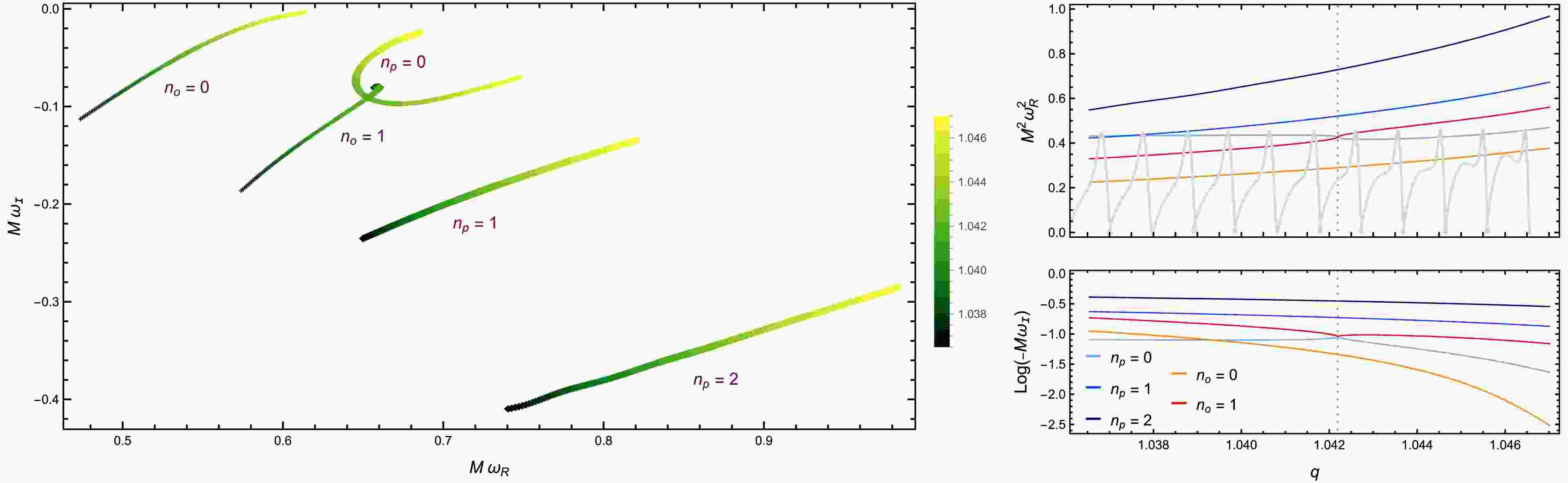
$ \alpha=\alpha_{\mathrm{EP}} $ in Fig. 1. The left panel shows the trajectories of the QNM frequencies in the complex ω plane as q varies. The color bar indicates the value of q, with darker green corresponding to smaller q. The spectrum is organized into five distinct branches, two of which meet at the EP located at$ q=q_{\mathrm{EP}} $ . These QNM branches can be further classified into peak and off-peak modes, labeled by$ n_{p} $ and$ n_{o} $ , respectively [69]. A notable feature is that each of the two branches participating in the EP is divided by the EP into an upper and a lower segment. The two upper segments recombine to form the branch labeled by$ n_{p}=0 $ , whereas the two lower segments recombine to form the branch labeled by$ n_{o}=1 $ . This branch reorganization reflects the local square-root structure of the non-Hermitian spectrum near the EP and is consistent with mode-switching or hysteretic behavior under parameter variation around an EP [40]. Hereafter, we refer to the two modes involved in the spectral coalescence, namely the$ n_{p}=0 $ and$ n_{o}=1 $ modes, as the EP modes.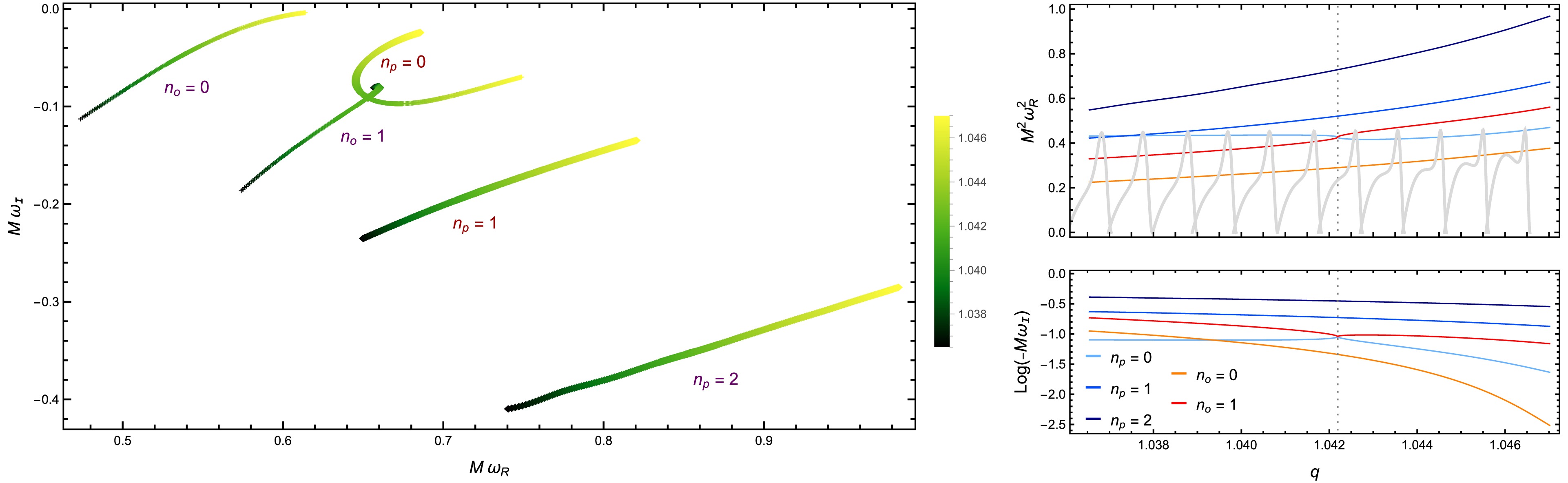
Figure 1. (color online) QNM spectrum of the test scalar field at
$ \alpha=\alpha_{\mathrm{EP}} $ for$ l=2 $ . Left: Trajectories of the QNM frequencies in the complex ω plane as the black-hole charge q is varied. The color bar indicates the value of q. The spectrum is organized into five branches, two of which meet at an EP at$ q=q_{\mathrm{EP} } $ . Near the EP, each of the two participating branches splits into upper and lower segments; the two upper (lower) segments recombine into the branch labeled by$ n_{p}=0 $ ($ n_{o}=1 $ ). Peak and off-peak modes are indexed by$ n_{p} $ and$ n_{o} $ , respectively. Upper right: Squared real part of the QNM frequencies,$ \omega_{R}^{2} $ , as a function of q. The gray dotted line marks$ q_{\mathrm{EP}} $ , where the real parts of the$ n_{p}=0 $ and$ n_{o}=1 $ branches cross. The panel also shows the effective potential$ V_{\mathrm{eff}} $ for several representative values of q, with each curve aligned so that its highest peak corresponds to the selected value of q. As q increases,$ V_{\mathrm{eff}} $ changes from a single-peaked to a double-peaked structure. In the single-peak regime, peak and off-peak modes are distinguished by the location of$ \omega_{R}^{2} $ : the former lie close to the peak value of$ V_{\mathrm{eff}} $ , whereas the latter have values appreciably below it. Lower right: Imaginary part of the QNM frequencies as a function of q. At$ q=q_{\mathrm{EP}} $ , the imaginary parts of the$ n_{p}=0 $ and$ n_{o}=1 $ modes coincide.The coalescence of this particular pair can be understood from the QNM spectrum of EMS hairy BHs analyzed in [69]. Off-peak modes undergo substantially larger spectral shifts as q varies than the relatively stable low-lying peak modes. In the relevant parameter region, the
$ n_p=0 $ and$ n_o=1 $ modes are the closest pair drawn from the two families. The stronger migration of the$ n_o=1 $ mode therefore brings it into resonance with the$ n_p=0 $ mode as the background parameters vary, allowing the two modes to coalesce at the EP.The upper-right and lower-right panels of Fig. 1 show
$ (M\omega_{R})^{2} $ and$ \log(-M\omega_{I}) $ as functions of q, respectively, where$ \omega_{R}\equiv\mathrm{Re}(\omega) $ and$ \omega _{I}\equiv\mathrm{Im}(\omega) $ . The value of$ q_{\mathrm{EP}} $ is marked by the gray dotted line. The upper-right panel shows that the squared real components of the frequencies of the$ n_{p}=0 $ and$ n_{o}=1 $ branches cross at$ q=q_{\mathrm{EP}} $ . The same panel also displays the effective potential$ V_{\mathrm{eff}} $ for several representative values of q. For sufficiently small q, the effective potential has a single peak. The peak and off-peak modes labeled by$ n_{p} $ and$ n_{o} $ correspond to modes localized near the potential peak and appreciably below it, respectively.1 The peak and off-peak modes are ordered according to their decay rates, with
$ n_{p}=0 $ and$ n_{o}=0 $ denoting the least damped peak and off-peak modes, respectively. As shown in the lower-right panel, increasing q causes the$ n_{p}=0 $ and$ n_{o}=0 $ modes to undergo fundamental-mode overtaking. In addition, the imaginary parts of the frequencies of the$ n_{p}=0 $ and$ n_{o}=1 $ modes coincide at$ q=q_{\mathrm{EP}} $ . At$ q=q_{\mathrm{EP}} $ , the fundamental mode is the$ n_{o}=0 $ mode, whereas the EP modes constitute the lowest overtone. The lower-right panel also shows that branch reorganization occurs for the$ n_{p}=0 $ and$ n_{o}=1 $ modes near the EP. The branch reorganization shown in the left panel, together with the behavior of$ (M\omega_R)^2 $ in the upper-right panel, indicates an exchange of mode character across the EP. Tracing the two local spectral trajectories through the near-EP region shows that their values of$ (M\omega_R)^2 $ are characteristic of peak and off-peak modes, respectively, for$ q<q_{\rm{EP}} $ , whereas this correspondence is reversed for$ q>q_{\rm{EP}} $ . The branch reorganization can therefore be interpreted as an exchange of peak/off-peak character between the two modes.To further resolve the QNM behavior in the immediate vicinity of the EP, Fig. 2 shows the dependence of both the frequency splitting and the eigenfunction mismatch on q for the
$ n_{p}=0 $ and$ n_{o}=1 $ modes. The left panel displays the squared frequency splitting,$ \delta \omega^{2}\equiv\left\vert \omega_{1}^{o}-\omega_{0}^{p}\right\vert ^{2} $ , as a function of q near$ q_{\mathrm{EP}} $ , indicated by the gray dotted line. We observe a pronounced cusp at$ q=q_{\mathrm{EP}} $ :$ \delta\omega^{2} $ decreases approximately linearly as q approaches$ q_{\mathrm{EP}} $ from either side and increases again after passing through the EP. This behavior is characteristic of a second-order EP, where the local eigenvalue splitting scales as the square root of the control parameter; consequently, the squared splitting becomes linear sufficiently close to the EP [40]. At$ q=q_{\mathrm{EP}} $ , the numerical splitting does not vanish identically but remains below our numerical tolerance of$ 10^{-6} $ .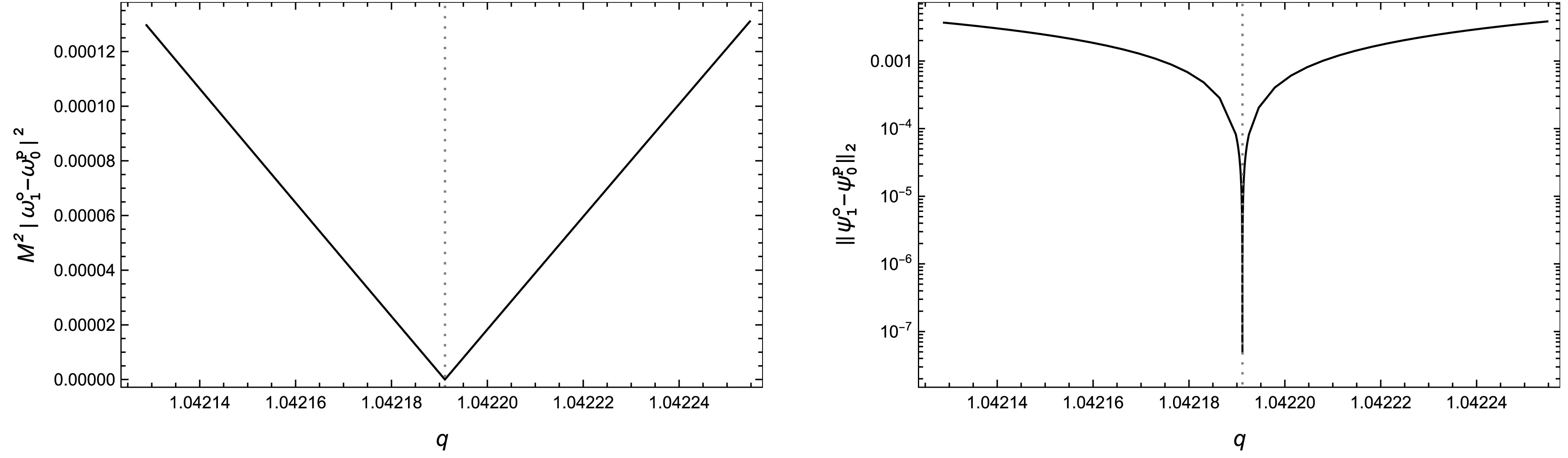
Figure 2. Squared difference between the QNM frequencies
$ \omega_{0}^{p} $ and$ \omega_{1}^{o} $ for the$ n_{p}=0 $ and$ n_{o}=1 $ modes (Left), and the$ L^{2} $ norm of the difference between the corresponding eigenfunctions$ \psi_{1}^{o} $ and$ \psi_{0}^{p} $ (Right), as functions of the BH charge q. In both panels, the gray dotted line indicates the EP location at$ q=q_{\mathrm{EP}} $ . As q approaches$ q_{\mathrm{EP}} $ , the squared frequency difference decreases approximately linearly to an extremely small value, whereas the eigenfunction difference decreases sharply, indicating the near coalescence of the two eigenfunctions. The simultaneous strong suppression of the eigenvalue and eigenfunction differences provides direct numerical evidence for the EP in the QNM spectrum.The right panel shows the corresponding
$ L^{2} $ mismatch$ \left\Vert \psi _{1}^{o}-\psi_{0}^{p}\right\Vert _{2} $ between the two eigenfunctions$ \psi_{1}^{o} $ and$ \psi_{0}^{p} $ . As q approaches$ q_{\mathrm{EP}} $ , this quantity decreases sharply to an extremely small value, indicating that the two eigenfunctions become nearly indistinguishable. The simultaneous near-vanishing of the eigenvalue splitting and the eigenfunction mismatch provides direct numerical evidence for the coalescence of both eigenvalues and eigenfunctions, which is the defining signature of an EP in a non-Hermitian QNM problem. Away from the exact EP, the degeneracy is lifted continuously: the two modes acquire a finite frequency splitting, and their eigenfunctions become distinguishable. Thus, nearby values of$ (\alpha,q) $ do not produce an abrupt change in the spectrum but instead exhibit a continuous crossover from the coalesced EP to two distinct QNMs. -
The emergence of an EP in the QNM spectrum is generally associated with the variation of at least two control parameters in the underlying non-Hermitian eigenvalue problem. In the EMS model, this requirement is naturally satisfied by the coupling constant α and the BH charge q. Motivated by this structure, in this section we perform a frequency-domain search for EPs in the QNM spectrum. Our strategy is to fix α and scan over q to track the evolution of adjacent QNM branches. If no coalescence is observed, we then adjust α and repeat the scan. Following this procedure, for
$ l=2 $ we identify a numerically resolved coalescence point at$ \alpha=\alpha_{\mathrm{EP}}\simeq $ 0.79040751953125 and$ q=q_{\mathrm{EP}}\simeq1.0421911480 $ . Because the numerical location of an exact EP is necessarily limited by the spectral resolution, the parameter search, and the coalescence criterion, the full numerical values quoted here specify the parameter point used in our calculations rather than mathematically exact EP coordinates. Within our numerical accuracy, we refer to this point as the EP hereafter. The convergence tests supporting this identification are presented in the Appendix.We show the QNM spectrum at
$ \alpha=\alpha_{\mathrm{EP}} $ in Fig. 1. The left panel shows the trajectories of the QNM frequencies in the complex ω plane as q varies. The color bar indicates the value of q, with darker green corresponding to smaller q. The spectrum is organized into five distinct branches, two of which meet at the EP located at$ q=q_{\mathrm{EP}} $ . These QNM branches can be further classified into peak and off-peak modes, labeled by$ n_{p} $ and$ n_{o} $ , respectively [69]. A notable feature is that each of the two branches participating in the EP is divided by the EP into an upper and a lower segment. The two upper segments recombine to form the branch labeled by$ n_{p}=0 $ , whereas the two lower segments recombine to form the branch labeled by$ n_{o}=1 $ . This branch reorganization reflects the local square-root structure of the non-Hermitian spectrum near the EP and is consistent with mode-switching or hysteretic behavior under parameter variation around an EP [40]. Hereafter, we refer to the two modes involved in the spectral coalescence, namely the$ n_{p}=0 $ and$ n_{o}=1 $ modes, as the EP modes.
Figure 1. (color online) QNM spectrum of the test scalar field at
$ \alpha=\alpha_{\mathrm{EP}} $ for$ l=2 $ . Left: Trajectories of the QNM frequencies in the complex ω plane as the black-hole charge q is varied. The color bar indicates the value of q. The spectrum is organized into five branches, two of which meet at an EP at$ q=q_{\mathrm{EP} } $ . Near the EP, each of the two participating branches splits into upper and lower segments; the two upper (lower) segments recombine into the branch labeled by$ n_{p}=0 $ ($ n_{o}=1 $ ). Peak and off-peak modes are indexed by$ n_{p} $ and$ n_{o} $ , respectively. Upper right: Squared real part of the QNM frequencies,$ \omega_{R}^{2} $ , as a function of q. The gray dotted line marks$ q_{\mathrm{EP}} $ , where the real parts of the$ n_{p}=0 $ and$ n_{o}=1 $ branches cross. The panel also shows the effective potential$ V_{\mathrm{eff}} $ for several representative values of q, with each curve aligned so that its highest peak corresponds to the selected value of q. As q increases,$ V_{\mathrm{eff}} $ changes from a single-peaked to a double-peaked structure. In the single-peak regime, peak and off-peak modes are distinguished by the location of$ \omega_{R}^{2} $ : the former lie close to the peak value of$ V_{\mathrm{eff}} $ , whereas the latter have values appreciably below it. Lower right: Imaginary part of the QNM frequencies as a function of q. At$ q=q_{\mathrm{EP}} $ , the imaginary parts of the$ n_{p}=0 $ and$ n_{o}=1 $ modes coincide.The coalescence of this particular pair can be understood from the QNM spectrum of EMS hairy BHs analyzed in [69]. Off-peak modes undergo substantially larger spectral shifts as q varies than the relatively stable low-lying peak modes. In the relevant parameter region, the
$ n_p=0 $ and$ n_o=1 $ modes are the closest pair drawn from the two families. The stronger migration of the$ n_o=1 $ mode therefore brings it into resonance with the$ n_p=0 $ mode as the background parameters vary, allowing the two modes to coalesce at the EP.The upper-right and lower-right panels of Fig. 1 show
$ (M\omega_{R})^{2} $ and$ \log(-M\omega_{I}) $ as functions of q, respectively, where$ \omega_{R}\equiv\mathrm{Re}(\omega) $ and$ \omega _{I}\equiv\mathrm{Im}(\omega) $ . The value of$ q_{\mathrm{EP}} $ is marked by the gray dotted line. The upper-right panel shows that the squared real components of the frequencies of the$ n_{p}=0 $ and$ n_{o}=1 $ branches cross at$ q=q_{\mathrm{EP}} $ . The same panel also displays the effective potential$ V_{\mathrm{eff}} $ for several representative values of q. For sufficiently small q, the effective potential has a single peak. The peak and off-peak modes labeled by$ n_{p} $ and$ n_{o} $ correspond to modes localized near the potential peak and appreciably below it, respectively.1 The peak and off-peak modes are ordered according to their decay rates, with
$ n_{p}=0 $ and$ n_{o}=0 $ denoting the least damped peak and off-peak modes, respectively. As shown in the lower-right panel, increasing q causes the$ n_{p}=0 $ and$ n_{o}=0 $ modes to undergo fundamental-mode overtaking. In addition, the imaginary parts of the frequencies of the$ n_{p}=0 $ and$ n_{o}=1 $ modes coincide at$ q=q_{\mathrm{EP}} $ . At$ q=q_{\mathrm{EP}} $ , the fundamental mode is the$ n_{o}=0 $ mode, whereas the EP modes constitute the lowest overtone. The lower-right panel also shows that branch reorganization occurs for the$ n_{p}=0 $ and$ n_{o}=1 $ modes near the EP. The branch reorganization shown in the left panel, together with the behavior of$ (M\omega_R)^2 $ in the upper-right panel, indicates an exchange of mode character across the EP. Tracing the two local spectral trajectories through the near-EP region shows that their values of$ (M\omega_R)^2 $ are characteristic of peak and off-peak modes, respectively, for$ q<q_{\rm{EP}} $ , whereas this correspondence is reversed for$ q>q_{\rm{EP}} $ . The branch reorganization can therefore be interpreted as an exchange of peak/off-peak character between the two modes.To further resolve the QNM behavior in the immediate vicinity of the EP, Fig. 2 shows the dependence of both the frequency splitting and the eigenfunction mismatch on q for the
$ n_{p}=0 $ and$ n_{o}=1 $ modes. The left panel displays the squared frequency splitting,$ \delta \omega^{2}\equiv\left\vert \omega_{1}^{o}-\omega_{0}^{p}\right\vert ^{2} $ , as a function of q near$ q_{\mathrm{EP}} $ , indicated by the gray dotted line. We observe a pronounced cusp at$ q=q_{\mathrm{EP}} $ :$ \delta\omega^{2} $ decreases approximately linearly as q approaches$ q_{\mathrm{EP}} $ from either side and increases again after passing through the EP. This behavior is characteristic of a second-order EP, where the local eigenvalue splitting scales as the square root of the control parameter; consequently, the squared splitting becomes linear sufficiently close to the EP [40]. At$ q=q_{\mathrm{EP}} $ , the numerical splitting does not vanish identically but remains below our numerical tolerance of$ 10^{-6} $ .
Figure 2. Squared difference between the QNM frequencies
$ \omega_{0}^{p} $ and$ \omega_{1}^{o} $ for the$ n_{p}=0 $ and$ n_{o}=1 $ modes (Left), and the$ L^{2} $ norm of the difference between the corresponding eigenfunctions$ \psi_{1}^{o} $ and$ \psi_{0}^{p} $ (Right), as functions of the BH charge q. In both panels, the gray dotted line indicates the EP location at$ q=q_{\mathrm{EP}} $ . As q approaches$ q_{\mathrm{EP}} $ , the squared frequency difference decreases approximately linearly to an extremely small value, whereas the eigenfunction difference decreases sharply, indicating the near coalescence of the two eigenfunctions. The simultaneous strong suppression of the eigenvalue and eigenfunction differences provides direct numerical evidence for the EP in the QNM spectrum.The right panel shows the corresponding
$ L^{2} $ mismatch$ \left\Vert \psi _{1}^{o}-\psi_{0}^{p}\right\Vert _{2} $ between the two eigenfunctions$ \psi_{1}^{o} $ and$ \psi_{0}^{p} $ . As q approaches$ q_{\mathrm{EP}} $ , this quantity decreases sharply to an extremely small value, indicating that the two eigenfunctions become nearly indistinguishable. The simultaneous near-vanishing of the eigenvalue splitting and the eigenfunction mismatch provides direct numerical evidence for the coalescence of both eigenvalues and eigenfunctions, which is the defining signature of an EP in a non-Hermitian QNM problem. Away from the exact EP, the degeneracy is lifted continuously: the two modes acquire a finite frequency splitting, and their eigenfunctions become distinguishable. Thus, nearby values of$ (\alpha,q) $ do not produce an abrupt change in the spectrum but instead exhibit a continuous crossover from the coalesced EP to two distinct QNMs. -
In this section, we extract QNMs from the time-domain waveform at
$ \alpha=\alpha_{\mathrm{EP}} $ and$ q=q_{\mathrm{EP}} $ , where the frequency-domain analysis indicates the presence of an EP associated with the coalescence of two spectral branches. The waveform used for the extraction is shown in Fig. 3. We consider both the standard and EP ansatzes, given in Eqs. (17) and (18), respectively, to assess the effect of the ansatz choice on the extracted frequencies and amplitudes. The extraction is performed using both the weak-fit and strong-fit schemes. For each scheme, we repeat the fit while varying the start time$ t_{0} $ over the interval$ (t_{0}-t_{\mathrm{peak}})/M\in\lbrack0,130] $ . Here,$ t_{\mathrm{peak} } $ denotes the time at which the waveform amplitude reaches its maximum.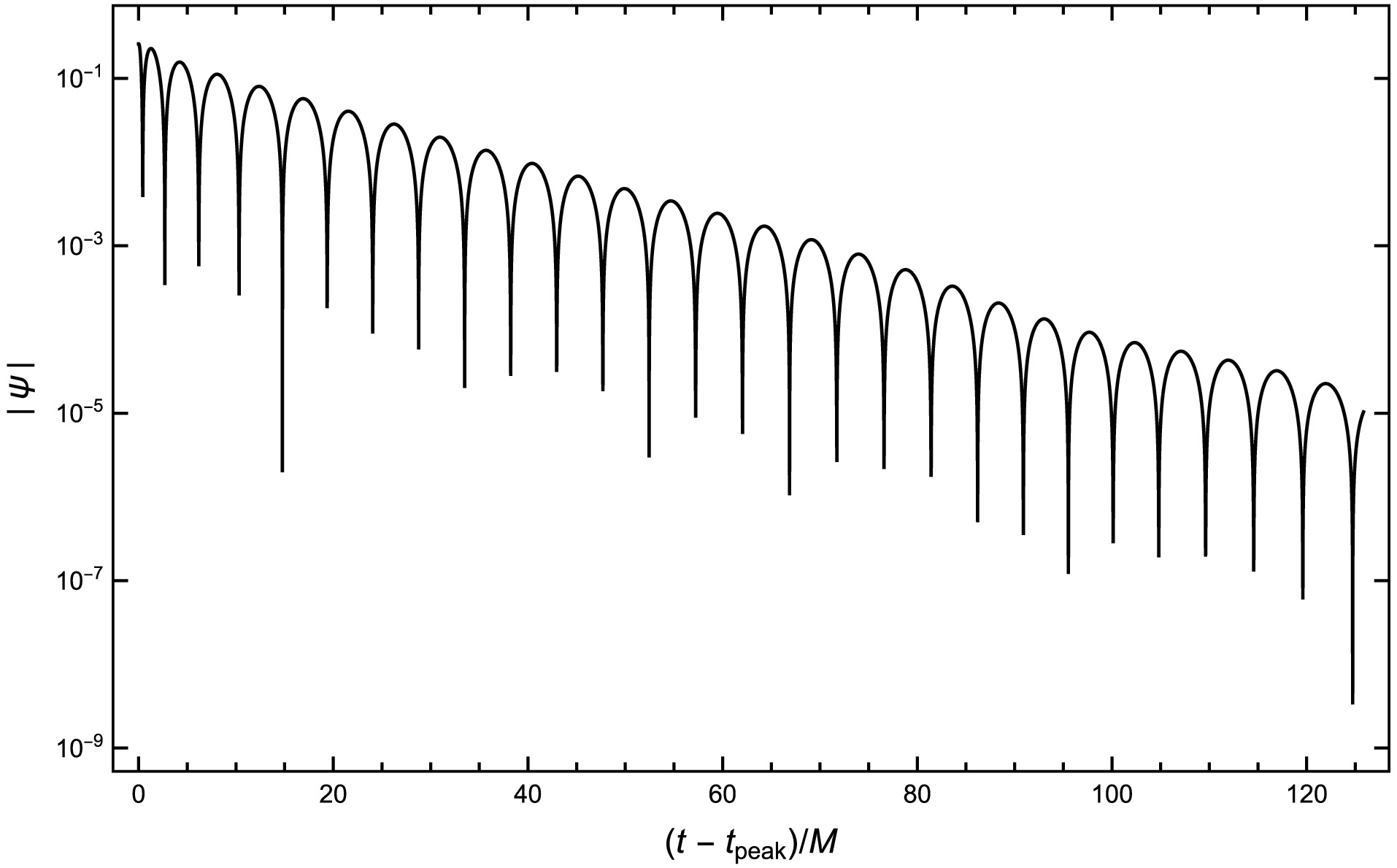
Figure 3. The time-domain ringdown waveform ψ of the scalar field at
$ \alpha=\alpha_{\mathrm{EP}} $ and$ q=q_{\mathrm{EP}} $ is plotted as a function of$ (t-t_{\mathrm{peak}})/M $ . Here,$ t_{\mathrm{peak}} $ denotes the time at which the waveform amplitude reaches its maximum. The observer is located at$ r=27.452M $ . -
In this section, we extract QNMs from the time-domain waveform at
$ \alpha=\alpha_{\mathrm{EP}} $ and$ q=q_{\mathrm{EP}} $ , where the frequency-domain analysis indicates the presence of an EP associated with the coalescence of two spectral branches. The waveform used for the extraction is shown in Fig. 3. We consider both the standard and EP ansatzes, given in Eqs. (17) and (18), respectively, to assess the effect of the ansatz choice on the extracted frequencies and amplitudes. The extraction is performed using both the weak-fit and strong-fit schemes. For each scheme, we repeat the fit while varying the start time$ t_{0} $ over the interval$ (t_{0}-t_{\mathrm{peak}})/M\in\lbrack0,130] $ . Here,$ t_{\mathrm{peak} } $ denotes the time at which the waveform amplitude reaches its maximum.
Figure 3. The time-domain ringdown waveform ψ of the scalar field at
$ \alpha=\alpha_{\mathrm{EP}} $ and$ q=q_{\mathrm{EP}} $ is plotted as a function of$ (t-t_{\mathrm{peak}})/M $ . Here,$ t_{\mathrm{peak}} $ denotes the time at which the waveform amplitude reaches its maximum. The observer is located at$ r=27.452M $ . -
We first apply the weak-fitting scheme based on the standard ansatz in Eq. (17) to extract the amplitudes and phases from the time-domain waveform. In this fit, we include the four least damped modes, namely the
$ n_{p}=0,1 $ peak modes and the$ n_{o}=0,1 $ off-peak modes, with their frequencies fixed by the frequency-domain analysis. The left and right panels of Fig. 4 show the extracted amplitudes$ A_{n} $ and phases$ \phi_{n} $ , respectively, as functions of the start time$ (t_{0}-t_{\mathrm{peak}})/M $ . For three of the four modes, namely$ n_{p}=0 $ ,$ n_{o}=0 $ , and$ n_{o}=1 $ , both the amplitudes and phases approach well-defined plateaus for$ (t_{0}-t_{\mathrm{peak}})/M\gtrsim20 $ , indicating that these modes can be extracted reliably within this time window. By contrast, the$ n_{p}=1 $ mode exhibits a substantially stronger dependence on$ t_{0} $ . Because it is the most strongly damped of the four modes, its extraction is feasible only over a relatively early interval, roughly$ 20\lesssim(t_{0}-t_{\mathrm{peak}})/M\lesssim40 $ , and is therefore less robust.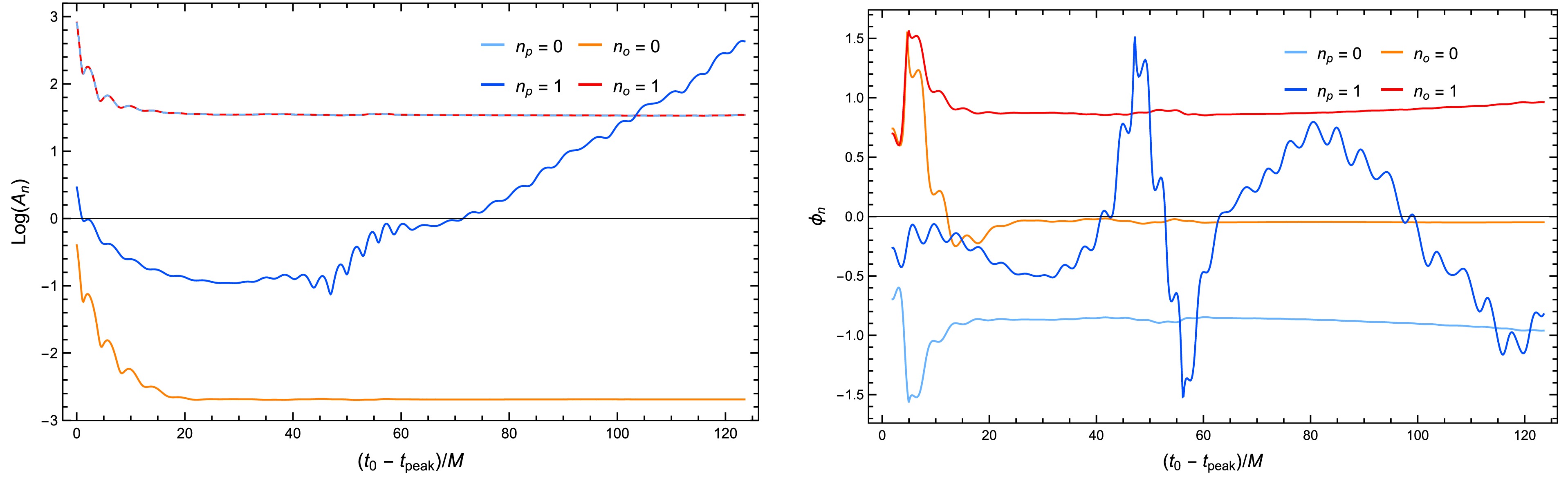
Figure 4. (color online) Extracted amplitudes
$ A_{n} $ (Left) and phases$ \phi_{n} $ (Right) obtained with the standard ansatz, plotted as functions of the starting time$ (t_{0} -t_{\mathrm{peak}})/M $ . The fit includes the four least damped modes, namely the$ n_{p}=0,1 $ peak modes and the$ n_{o}=0,1 $ off-peak modes, with frequencies fixed by the frequency-domain analysis. The two EP modes,$ n_{p}=0 $ and$ n_{o}=1 $ , have nearly equal amplitudes and dominate over the other fitted modes. Their phases are approximately opposite, indicating destructive interference between their contributions.A particularly notable feature is that the EP modes, namely the
$ n_{p}=0 $ and$ n_{o}=1 $ modes, have nearly equal extracted amplitudes, both exceeding those of the other two modes by at least two orders of magnitude. This hierarchy indicates that the contribution from each individual EP mode is strongly enhanced in the ringdown signal. At the same time, these two dominant modes have approximately opposite phases, so their contributions nearly cancel in the waveform. This pattern is consistent with recent analyses of ringdown near an EP, in which the resonant pair is strongly amplified, while destructive interference between the dominant components suppresses the net contribution to the waveform [52].We next repeat the weak-fit analysis using the EP ansatz, in which the two EP modes are replaced by a single EP contribution, while the nonresonant modes
$ n_{o}=0 $ and$ n_{p}=1 $ are retained explicitly. The left and right panels of Fig. 5 show the extracted amplitudes and phases, respectively, as functions of the starting time$ (t_{0}-t_{\mathrm{peak}})/M $ . A notable feature is that the EP contribution can be cleanly decomposed into a time-independent term and a term linear in time, both of which exhibit relatively stable plateaus over a broad fitting window. In contrast to the standard ansatz, in which the two EP modes are treated separately and acquire very large extracted amplitudes, the EP ansatz absorbs their combined effect into a single resonant contribution with substantially smaller coefficients. This behavior indicates that the large amplitudes found in Fig. 4 arise primarily from forcing the nearly coalescing pair into two independent QNMs, whereas the EP ansatz captures the ringdown more economically in terms of the resonant structure near the EP. It is also worth noting that the time-independent and time-linear EP terms have almost identical phases, so they add nearly in phase and together form a coherent resonant contribution. Overall, Fig. 5 shows that the EP ansatz provides a more natural and stable description of the waveform in the near-EP regime. Moreover, since the$ n_{o}=0 $ fundamental mode belongs to the off-peak family and is spectrally less stable, its contribution is suppressed relative to the EP contribution [69].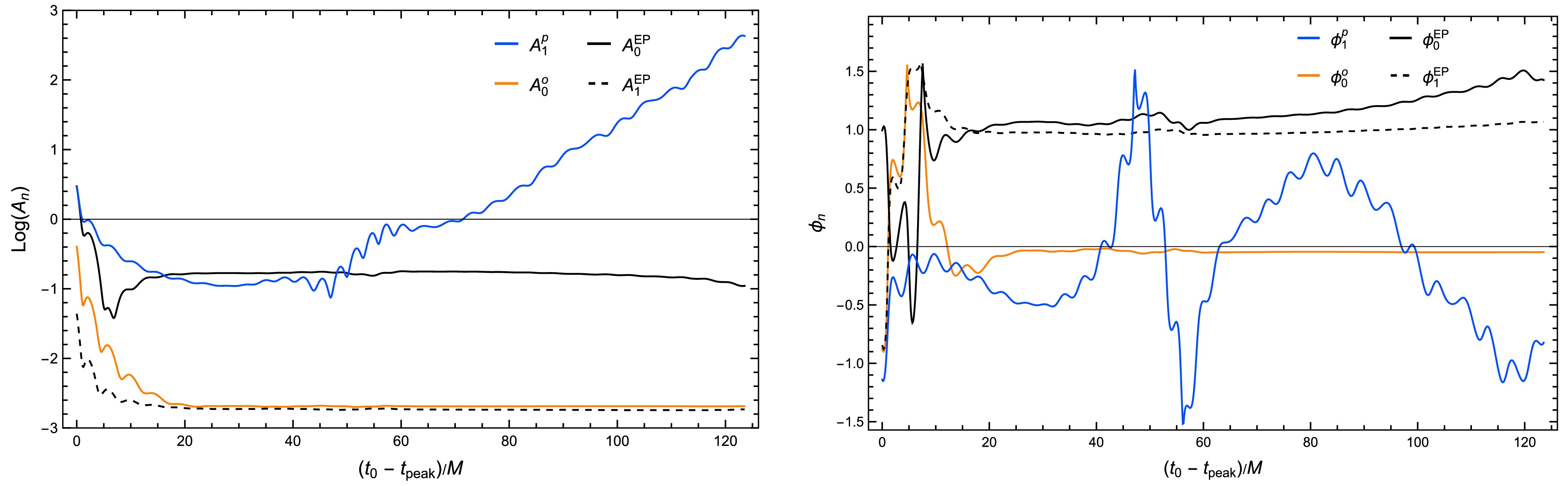
Figure 5. (color online) The extracted amplitudes
$ A_{n} $ (Left) and phases$ \phi_{n} $ (Right) obtained with the EP ansatz are shown as functions of the start time$ (t_{0}-t_{\mathrm{peak} })/M $ . The fit includes two nonresonant modes,$ n_{o}=0 $ and$ n_{p}=1 $ , together with the EP contribution, with frequencies fixed by the frequency-domain analysis. The EP contribution is decomposed into a time-independent term (solid black) and a term linear in time (dashed black). Their amplitudes are substantially smaller than the individual amplitudes of the EP modes obtained with the standard ansatz in Fig. 4, indicating that the EP ansatz provides a more economical description of the near-EP ringdown. -
We first apply the weak-fitting scheme based on the standard ansatz in Eq. (17) to extract the amplitudes and phases from the time-domain waveform. In this fit, we include the four least damped modes, namely the
$ n_{p}=0,1 $ peak modes and the$ n_{o}=0,1 $ off-peak modes, with their frequencies fixed by the frequency-domain analysis. The left and right panels of Fig. 4 show the extracted amplitudes$ A_{n} $ and phases$ \phi_{n} $ , respectively, as functions of the start time$ (t_{0}-t_{\mathrm{peak}})/M $ . For three of the four modes, namely$ n_{p}=0 $ ,$ n_{o}=0 $ , and$ n_{o}=1 $ , both the amplitudes and phases approach well-defined plateaus for$ (t_{0}-t_{\mathrm{peak}})/M\gtrsim20 $ , indicating that these modes can be extracted reliably within this time window. By contrast, the$ n_{p}=1 $ mode exhibits a substantially stronger dependence on$ t_{0} $ . Because it is the most strongly damped of the four modes, its extraction is feasible only over a relatively early interval, roughly$ 20\lesssim(t_{0}-t_{\mathrm{peak}})/M\lesssim40 $ , and is therefore less robust.
Figure 4. (color online) Extracted amplitudes
$ A_{n} $ (Left) and phases$ \phi_{n} $ (Right) obtained with the standard ansatz, plotted as functions of the starting time$ (t_{0} -t_{\mathrm{peak}})/M $ . The fit includes the four least damped modes, namely the$ n_{p}=0,1 $ peak modes and the$ n_{o}=0,1 $ off-peak modes, with frequencies fixed by the frequency-domain analysis. The two EP modes,$ n_{p}=0 $ and$ n_{o}=1 $ , have nearly equal amplitudes and dominate over the other fitted modes. Their phases are approximately opposite, indicating destructive interference between their contributions.A particularly notable feature is that the EP modes, namely the
$ n_{p}=0 $ and$ n_{o}=1 $ modes, have nearly equal extracted amplitudes, both exceeding those of the other two modes by at least two orders of magnitude. This hierarchy indicates that the contribution from each individual EP mode is strongly enhanced in the ringdown signal. At the same time, these two dominant modes have approximately opposite phases, so their contributions nearly cancel in the waveform. This pattern is consistent with recent analyses of ringdown near an EP, in which the resonant pair is strongly amplified, while destructive interference between the dominant components suppresses the net contribution to the waveform [52].We next repeat the weak-fit analysis using the EP ansatz, in which the two EP modes are replaced by a single EP contribution, while the nonresonant modes
$ n_{o}=0 $ and$ n_{p}=1 $ are retained explicitly. The left and right panels of Fig. 5 show the extracted amplitudes and phases, respectively, as functions of the starting time$ (t_{0}-t_{\mathrm{peak}})/M $ . A notable feature is that the EP contribution can be cleanly decomposed into a time-independent term and a term linear in time, both of which exhibit relatively stable plateaus over a broad fitting window. In contrast to the standard ansatz, in which the two EP modes are treated separately and acquire very large extracted amplitudes, the EP ansatz absorbs their combined effect into a single resonant contribution with substantially smaller coefficients. This behavior indicates that the large amplitudes found in Fig. 4 arise primarily from forcing the nearly coalescing pair into two independent QNMs, whereas the EP ansatz captures the ringdown more economically in terms of the resonant structure near the EP. It is also worth noting that the time-independent and time-linear EP terms have almost identical phases, so they add nearly in phase and together form a coherent resonant contribution. Overall, Fig. 5 shows that the EP ansatz provides a more natural and stable description of the waveform in the near-EP regime. Moreover, since the$ n_{o}=0 $ fundamental mode belongs to the off-peak family and is spectrally less stable, its contribution is suppressed relative to the EP contribution [69].
Figure 5. (color online) The extracted amplitudes
$ A_{n} $ (Left) and phases$ \phi_{n} $ (Right) obtained with the EP ansatz are shown as functions of the start time$ (t_{0}-t_{\mathrm{peak} })/M $ . The fit includes two nonresonant modes,$ n_{o}=0 $ and$ n_{p}=1 $ , together with the EP contribution, with frequencies fixed by the frequency-domain analysis. The EP contribution is decomposed into a time-independent term (solid black) and a term linear in time (dashed black). Their amplitudes are substantially smaller than the individual amplitudes of the EP modes obtained with the standard ansatz in Fig. 4, indicating that the EP ansatz provides a more economical description of the near-EP ringdown. -
In the strong-fit scheme, we extract not only the amplitudes
$ A_{n} $ and phases$ \phi_{n} $ , but also the frequencies$ \omega_{n} $ of the fitted modes. To assess the robustness of this extraction, we introduce the frequency deviation,$ \delta\omega_{n}\equiv\left\vert \omega_{n}-\omega_{\mathrm{FD} }^{n}\right\vert $ , which quantifies the difference between the frequency obtained from the time-domain fit and the corresponding frequency-domain value. For both the standard and EP ansatzes, we consider fits that include either one mode or two modes.We first examine the standard ansatz in Eq. (17). When only a single QNM is included in the fit, the only mode that can be extracted reliably is the one that asymptotically becomes the fundamental mode at late times. In this regime, the overtones, including the EP modes, have already decayed substantially, making their contributions to the waveform difficult to resolve.
The results of the two-mode fit with the standard ansatz are shown in Fig. 6. These results indicate that the frequencies of both the fundamental and EP modes can be extracted reliably for
$ (t_{0}-t_{\mathrm{peak}})/M\gtrsim20 $ . The left panel displays the extracted QNM frequencies in the complex ω plane for$ 115\lesssim(t_{0}-t_{\mathrm{peak}})/M\lesssim127 $ , where the frequency deviations$ \delta\omega $ are close to their minimum values. The inset further shows that the frequency deviation$ \delta\omega_{0} $ for the fundamental mode reaches a minimum of order$ 10^{-4} $ , whereas the corresponding deviation$ \delta\omega_{1} $ for the EP mode reaches a minimum of order$ 10^{-3} $ . Notably, the lower-right panel shows that, for$ (t_{0}-t_{\mathrm{peak}})/M\gtrsim20 $ , the extracted amplitude$ A_{0} $ of the fundamental mode remains approximately constant, whereas the extracted amplitude$ A_{1} $ of the EP mode increases almost linearly with the start time. This behavior is precisely what is expected from the time-linear term in the EP ansatz. In this sense, even when the waveform is fitted with the standard ansatz, the resulting fit tends to reproduce the characteristic structure encoded in the EP ansatz.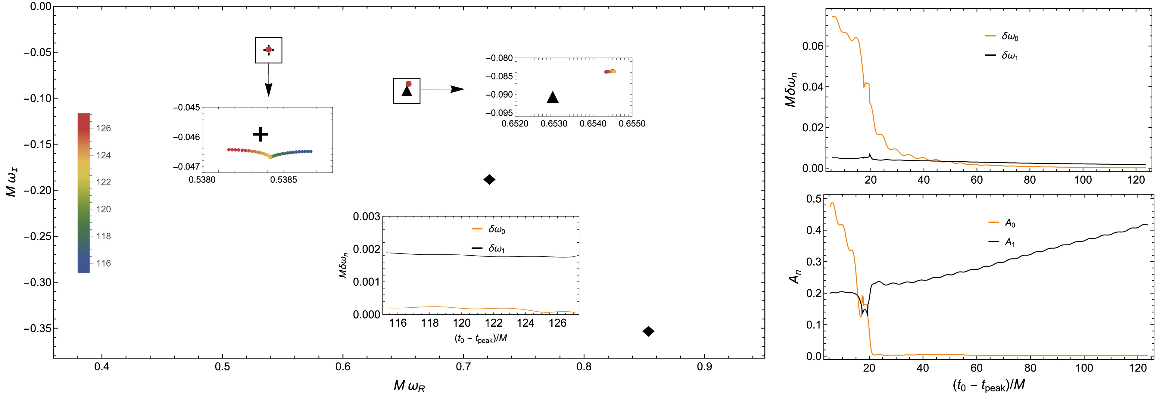
Figure 6. (color online) Results of the strong fit obtained using the standard ansatz with two included modes. Left: Extracted QNM frequencies in the complex ω plane for different start times, shown as shaded dots. The color bar indicates the start time. The plus, triangle, and diamond markers denote the frequency-domain values of the fundamental mode, the EP modes, and the peak-mode overtones, respectively. The frequencies of the fundamental and EP modes are extracted reliably. Upper right: Frequency deviations
$ \delta\omega_{0} $ and$ \delta\omega_{1} $ for the fundamental and EP modes, plotted as functions of$ (t_{0}-t_{\mathrm{peak}})/M $ . The inset in the left panel shows that their minimum values are of order$ 10^{-4} $ and$ 10^{-3} $ , respectively. Lower right: Extracted amplitudes$ A_{0} $ and$ A_{1} $ for the fundamental and EP modes, plotted as functions of$ (t_{0}-t_{\mathrm{peak} })/M $ . For$ (t_{0}-t_{\mathrm{peak}})/M\gtrsim20 $ ,$ A_{0} $ remains approximately constant, whereas$ A_{1} $ increases nearly linearly with the start time.Fig. 7 shows the strong-fit results obtained using the EP ansatz, including only the EP contribution. The lower-right panel displays the extracted amplitudes
$ A_{0}^{\mathrm{EP}} $ and$ A_{1}^{\mathrm{EP}} $ as functions of the start time. For$ (t_{0}-t_{\mathrm{peak}})/M\lesssim40 $ , both amplitudes remain approximately stable, indicating that, within this time window, the waveform can be described reasonably well by the EP contribution alone. At later times, however, the amplitudes become increasingly unstable, and the frequency deviation$ \delta\omega_{\mathrm{EP}} $ also increases. This behavior suggests that the EP ansatz containing only the EP terms is effective only over an early fitting window and becomes insufficient once the fundamental mode begins to dominate the waveform. The left panel shows the extracted frequencies in the complex ω plane as the start time varies over$ 14\lesssim(t_{0}-t_{\mathrm{peak}})/M\lesssim22 $ , indicating that the extracted frequencies remain close to the frequency-domain value of$ \omega_{\mathrm{EP}} $ . The inset further shows that the frequency deviation$ \delta\omega_{\mathrm{EP}} $ reaches a minimum on the order of$ 10^{-4} $ around$ (t_{0}-t_{\mathrm{peak}})/M\sim16 $ .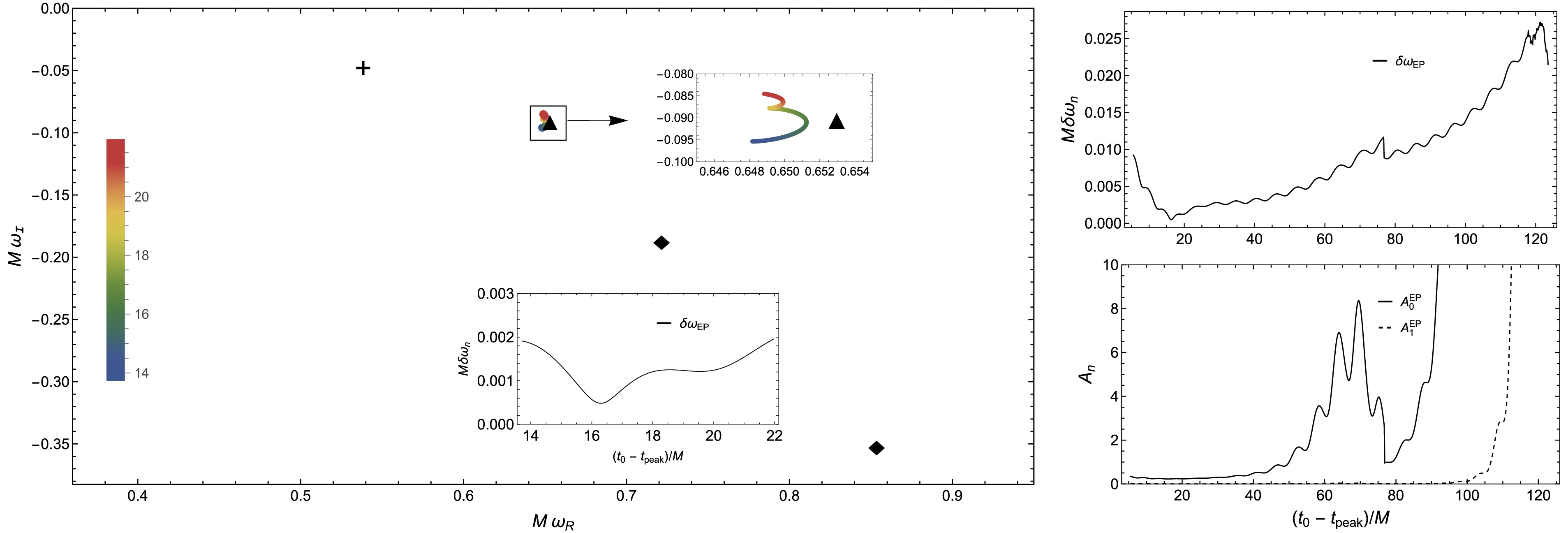
Figure 7. (color online) Results of the strong fit obtained using the EP ansatz with only the EP terms included. Left: Extracted frequencies in the complex ω plane for
$ 14\lesssim(t_{0}-t_{\mathrm{peak}})/M\lesssim22 $ . Throughout this interval, the extracted frequencies remain close to the frequency-domain value of$ \omega_{\mathrm{EP}} $ . The inset shows that the frequency deviation$ \delta\omega_{\mathrm{EP}} $ reaches a minimum of order$ 10^{-4} $ around$ (t_{0}-t_{\mathrm{peak}})/M\sim16 $ . The reference markers are the same as in Fig. 6. Upper right: Frequency deviation$ \delta \omega_{\mathrm{EP}} $ as a function of the start time. Lower right: Extracted amplitudes$ A_{0}^{\mathrm{EP}} $ and$ A_{1}^{\mathrm{EP}} $ as functions of the start time. For$ (t_{0}-t_{\mathrm{peak}})/M\lesssim40 $ , both amplitudes remain approximately stable, indicating that the fit is reliable within this time window. At later times, they become increasingly unstable, accompanied by an increase in$ \delta\omega_{\mathrm{EP}} $ .We finally consider the two-mode strong fit based on the EP ansatz, in which the waveform is described by the EP contribution together with one additional QNM contribution. The results are shown in Fig. 8. The left panel shows the extracted frequencies in the complex ω plane for
$ 40\lesssim(t_{0}-t_{\mathrm{peak}})/M\lesssim60 $ , demonstrating that the extracted frequencies are concentrated near the fundamental and EP modes. The inset shows that the minimum frequency deviations are of order$ 10^{-5} $ . Compared with the two-mode fit based on the standard ansatz, the minimum frequency deviations of the fundamental and EP modes are smaller by about one and two orders of magnitude, respectively. The lower-right panel shows the extracted amplitudes of the two contributions as functions of the start time, with the EP contribution decomposed into$ A_{0}^{\mathrm{EP}} $ and$ A_{1}^{\mathrm{EP}} $ . In contrast to the single-mode fit in Fig. 7, including the additional mode significantly improves the stability of the extraction and yields broad plateaus for both contributions. This indicates that, in this regime, the waveform is more accurately described by the combined contribution of the fundamental and EP modes.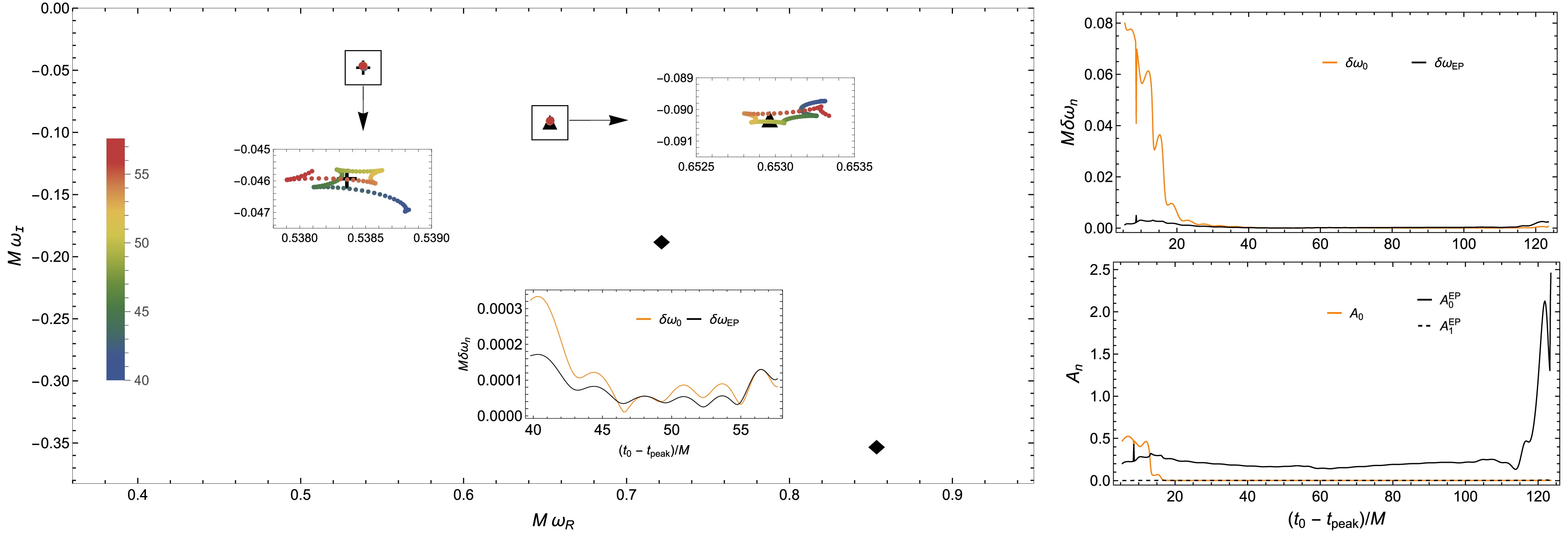
Figure 8. (color online) Results from the strong fit obtained with the two-mode EP ansatz. Left: Extracted frequencies in the complex ω plane as the start time varies over
$ 40\lesssim(t_{0}-t_{\mathrm{peak}})/M\lesssim60 $ , with the color bar indicating$ (t_{0}-t_{\mathrm{peak}})/M $ . The reference markers are the same as those in Fig. 6. The extracted frequencies cluster near the fundamental and EP modes. The inset shows that the minimum frequency deviations are of order$ 10^{-5} $ . Upper right: Frequency deviations$ \delta\omega_{0} $ and$ \delta\omega_{\mathrm{EP}} $ as functions of the start time. Lower right: Extracted amplitudes of the two contributions. The EP contribution is shown in black, with$ A_{0}^{\mathrm{EP}} $ plotted as a solid line and$ A_{1}^{\mathrm{EP}} $ as a dashed line. Compared with Fig. 7, including the additional mode leads to a more stable extraction and yields extended plateaus for both contributions.It is also useful to ask whether the time-domain behavior at the exact EP is qualitatively distinct from that at nearby parameter values. Away from the EP, the coalesced mode splits into two distinct QNMs. When the frequency splitting remains sufficiently small, however, the combined contribution of the two modes approaches the resonant behavior characteristic of the EP, which contains a term proportional to time [40]. Thus, one should not expect an abrupt change in the time-domain waveform when moving away from the exact EP. The distinctive structure of the exact EP is the resonant contribution proportional to time, whereas sufficiently near the EP, two closely spaced QNMs can mimic this behavior over a finite time interval. As the frequency splitting increases, the two modes become progressively distinguishable, and the waveform returns to the usual superposition of separate QNMs.
-
In the strong-fit scheme, we extract not only the amplitudes
$ A_{n} $ and phases$ \phi_{n} $ , but also the frequencies$ \omega_{n} $ of the fitted modes. To assess the robustness of this extraction, we introduce the frequency deviation,$ \delta\omega_{n}\equiv\left\vert \omega_{n}-\omega_{\mathrm{FD} }^{n}\right\vert $ , which quantifies the difference between the frequency obtained from the time-domain fit and the corresponding frequency-domain value. For both the standard and EP ansatzes, we consider fits that include either one mode or two modes.We first examine the standard ansatz in Eq. (17). When only a single QNM is included in the fit, the only mode that can be extracted reliably is the one that asymptotically becomes the fundamental mode at late times. In this regime, the overtones, including the EP modes, have already decayed substantially, making their contributions to the waveform difficult to resolve.
The results of the two-mode fit with the standard ansatz are shown in Fig. 6. These results indicate that the frequencies of both the fundamental and EP modes can be extracted reliably for
$ (t_{0}-t_{\mathrm{peak}})/M\gtrsim20 $ . The left panel displays the extracted QNM frequencies in the complex ω plane for$ 115\lesssim(t_{0}-t_{\mathrm{peak}})/M\lesssim127 $ , where the frequency deviations$ \delta\omega $ are close to their minimum values. The inset further shows that the frequency deviation$ \delta\omega_{0} $ for the fundamental mode reaches a minimum of order$ 10^{-4} $ , whereas the corresponding deviation$ \delta\omega_{1} $ for the EP mode reaches a minimum of order$ 10^{-3} $ . Notably, the lower-right panel shows that, for$ (t_{0}-t_{\mathrm{peak}})/M\gtrsim20 $ , the extracted amplitude$ A_{0} $ of the fundamental mode remains approximately constant, whereas the extracted amplitude$ A_{1} $ of the EP mode increases almost linearly with the start time. This behavior is precisely what is expected from the time-linear term in the EP ansatz. In this sense, even when the waveform is fitted with the standard ansatz, the resulting fit tends to reproduce the characteristic structure encoded in the EP ansatz.
Figure 6. (color online) Results of the strong fit obtained using the standard ansatz with two included modes. Left: Extracted QNM frequencies in the complex ω plane for different start times, shown as shaded dots. The color bar indicates the start time. The plus, triangle, and diamond markers denote the frequency-domain values of the fundamental mode, the EP modes, and the peak-mode overtones, respectively. The frequencies of the fundamental and EP modes are extracted reliably. Upper right: Frequency deviations
$ \delta\omega_{0} $ and$ \delta\omega_{1} $ for the fundamental and EP modes, plotted as functions of$ (t_{0}-t_{\mathrm{peak}})/M $ . The inset in the left panel shows that their minimum values are of order$ 10^{-4} $ and$ 10^{-3} $ , respectively. Lower right: Extracted amplitudes$ A_{0} $ and$ A_{1} $ for the fundamental and EP modes, plotted as functions of$ (t_{0}-t_{\mathrm{peak} })/M $ . For$ (t_{0}-t_{\mathrm{peak}})/M\gtrsim20 $ ,$ A_{0} $ remains approximately constant, whereas$ A_{1} $ increases nearly linearly with the start time.Figure 7 shows the strong-fit results obtained using the EP ansatz, including only the EP contribution. The lower-right panel displays the extracted amplitudes
$ A_{0}^{\mathrm{EP}} $ and$ A_{1}^{\mathrm{EP}} $ as functions of the start time. For$ (t_{0}-t_{\mathrm{peak}})/ M\lesssim40 $ , both amplitudes remain approximately stable, indicating that, within this time window, the waveform can be described reasonably well by the EP contribution alone. At later times, however, the amplitudes become increasingly unstable, and the frequency deviation$ \delta\omega_{\mathrm{EP}} $ also increases. This behavior suggests that the EP ansatz containing only the EP terms is effective only over an early fitting window and becomes insufficient once the fundamental mode begins to dominate the waveform. The left panel shows the extracted frequencies in the complex ω plane as the start time varies over$ 14\lesssim(t_{0}-t_{\mathrm{peak}})/ M\lesssim22 $ , indicating that the extracted frequencies remain close to the frequency-domain value of$ \omega_{\mathrm{EP}} $ . The inset further shows that the frequency deviation$ \delta\omega_{\mathrm{EP}} $ reaches a minimum on the order of$ 10^{-4} $ around$ (t_{0}-t_{\mathrm{peak}})/M\sim16 $ .
Figure 7. (color online) Results of the strong fit obtained using the EP ansatz with only the EP terms included. Left: Extracted frequencies in the complex ω plane for
$ 14\lesssim(t_{0}-t_{\mathrm{peak}})/M\lesssim22 $ . Throughout this interval, the extracted frequencies remain close to the frequency-domain value of$ \omega_{\mathrm{EP}} $ . The inset shows that the frequency deviation$ \delta\omega_{\mathrm{EP}} $ reaches a minimum of order$ 10^{-4} $ around$ (t_{0}-t_{\mathrm{peak}})/M\sim16 $ . The reference markers are the same as in Fig. 6. Upper right: Frequency deviation$ \delta \omega_{\mathrm{EP}} $ as a function of the start time. Lower right: Extracted amplitudes$ A_{0}^{\mathrm{EP}} $ and$ A_{1}^{\mathrm{EP}} $ as functions of the start time. For$ (t_{0}-t_{\mathrm{peak}})/M\lesssim40 $ , both amplitudes remain approximately stable, indicating that the fit is reliable within this time window. At later times, they become increasingly unstable, accompanied by an increase in$ \delta\omega_{\mathrm{EP}} $ .We finally consider the two-mode strong fit based on the EP ansatz, in which the waveform is described by the EP contribution together with one additional QNM contribution. The results are shown in Fig. 8. The left panel shows the extracted frequencies in the complex ω plane for
$ 40\lesssim(t_{0}-t_{\mathrm{peak}})/M\lesssim60 $ , demonstrating that the extracted frequencies are concentrated near the fundamental and EP modes. The inset shows that the minimum frequency deviations are of order$ 10^{-5} $ . Compared with the two-mode fit based on the standard ansatz, the minimum frequency deviations of the fundamental and EP modes are smaller by about one and two orders of magnitude, respectively. The lower-right panel shows the extracted amplitudes of the two contributions as functions of the start time, with the EP contribution decomposed into$ A_{0}^{\mathrm{EP}} $ and$ A_{1}^{\mathrm{EP}} $ . In contrast to the single-mode fit in Fig. 7, including the additional mode significantly improves the stability of the extraction and yields broad plateaus for both contributions. This indicates that, in this regime, the waveform is more accurately described by the combined contribution of the fundamental and EP modes.
Figure 8. (color online) Results from the strong fit obtained with the two-mode EP ansatz. Left: Extracted frequencies in the complex ω plane as the start time varies over
$ 40\lesssim(t_{0}-t_{\mathrm{peak}})/M\lesssim60 $ , with the color bar indicating$ (t_{0}-t_{\mathrm{peak}})/M $ . The reference markers are the same as those in Fig. 6. The extracted frequencies cluster near the fundamental and EP modes. The inset shows that the minimum frequency deviations are of order$ 10^{-5} $ . Upper right: Frequency deviations$ \delta\omega_{0} $ and$ \delta\omega_{\mathrm{EP}} $ as functions of the start time. Lower right: Extracted amplitudes of the two contributions. The EP contribution is shown in black, with$ A_{0}^{\mathrm{EP}} $ plotted as a solid line and$ A_{1}^{\mathrm{EP}} $ as a dashed line. Compared with Fig. 7, including the additional mode leads to a more stable extraction and yields extended plateaus for both contributions.It is also useful to ask whether the time-domain behavior at the exact EP is qualitatively distinct from that at nearby parameter values. Away from the EP, the coalesced mode splits into two distinct QNMs. When the frequency splitting remains sufficiently small, however, the combined contribution of the two modes approaches the resonant behavior characteristic of the EP, which contains a term proportional to time [40]. Thus, one should not expect an abrupt change in the time-domain waveform when moving away from the exact EP. The distinctive structure of the exact EP is the resonant contribution proportional to time, whereas sufficiently near the EP, two closely spaced QNMs can mimic this behavior over a finite time interval. As the frequency splitting increases, the two modes become progressively distinguishable, and the waveform returns to the usual superposition of separate QNMs.
-
In this work, we investigated the QNM spectrum of a test massless scalar field on hairy BHs in EMS theory. By exploring the parameter space spanned by the coupling constant α and the BH charge q, we identified an EP in the frequency-domain spectrum at
$ \alpha=\alpha_{\mathrm{EP}} $ and$ q=q_{\mathrm{EP}} $ , where two QNMs coalesce. Our analysis showed that this coalescence occurs not only in the complex frequencies but also in the corresponding eigenfunctions. These results establish that EPs can arise in the scalar QNM spectra of hairy BHs and provide a concrete realization of non-Hermitian spectral degeneracies in BH perturbation theory.Because the QNM frequencies are complex, bringing a generic pair of modes into exact coalescence imposes two real conditions, corresponding to the vanishing of the real and imaginary parts of their frequency splitting. The two independent parameters
$ (\alpha,q) $ therefore generally need to be adjusted simultaneously, so exact second-order EPs are expected to occur at isolated points in the two-dimensional parameter space. This reflects the generic codimension-two nature of a second-order EP in a non-Hermitian spectrum, rather than additional fine-tuning specific to the EMS model considered here. Nevertheless, the associated near-EP behavior persists in a finite neighborhood of the exact EP. Whether analogous EPs arise in other EMS models or in other perturbation sectors must be examined case by case.We then investigated the time-domain signatures of the EP by extracting QNMs from the ringdown waveform at
$ \alpha=\alpha_{\mathrm{EP}} $ and$ q=q_{\mathrm{EP}} $ . Using both weak-fit and strong-fit schemes, we compared the standard ansatz, based on the usual superposition of QNMs, with the EP ansatz, which incorporates the resonant contribution associated with the spectral degeneracy. In the weak-fit analysis, with the frequencies fixed by the frequency-domain results, we found that the amplitudes of the two coalescing modes are much larger than those of the other modes, while destructive interference between their contributions strongly suppresses their net effect on the waveform. By contrast, the EP ansatz absorbs their combined effect into a single resonant contribution consisting of a time-independent term and a term linear in time, whose amplitudes are comparable to those of the other modes.In the strong-fit analysis, where the QNM frequencies are treated as fitting variables, the standard ansatz yields an amplitude that grows approximately linearly with the start time, reflecting the linear time dependence encoded in the EP ansatz. Moreover, the EP ansatz, especially in the two-mode fit, gives significantly smaller differences between the extracted frequencies and their frequency-domain counterparts. Together with the absence of the strong amplitude hierarchy found in the standard ansatz, these results indicate that the EP ansatz provides a more natural and robust description of ringdown signals near EPs.
Overall, our results show that EPs in QNM spectra are not merely features of the frequency-domain spectrum but can also leave characteristic signatures in ringdown signals. This highlights the importance of the non-Hermitian spectral structure underlying BH perturbations and suggests that EP-based descriptions may be useful for analyzing ringdown in systems with nearly degenerate QNMs. The exact EP identified here occurs at a specific point in the two-dimensional
$ (\alpha,q) $ parameter space and therefore requires tuning of both parameters. The existence of two independent parameters, however, does not by itself guarantee the presence of an EP in a given EMS model. Rather, our results suggest that when two interacting QNM branches are brought sufficiently close as the background parameters vary, the two-parameter space provides a natural setting in which they can be tuned to an isolated EP. Moreover, the associated near-EP resonant behavior persists in a finite neighborhood of the exact EP. Whether analogous spectral structures and EPs arise in other regions of the parameter space, in other perturbation sectors, or in other EMS models depends on the detailed QNM spectrum and must be investigated case by case.Another interesting extension is to consider a charged complex scalar field. Its charge provides an additional tunable parameter and modifies the coupling of the scalar perturbation to the electromagnetic background, which can substantially alter the migration and interaction of QNM branches. The enlarged parameter space may therefore support a richer EP structure, potentially including exceptional lines rather than isolated points, although the existence of such structures must again be determined from the detailed QNM spectrum. Possible extensions of the present work include exploring these possibilities and systematically investigating their implications for BH spectroscopy.
-
In this work, we investigated the QNM spectrum of a test massless scalar field on hairy BHs in EMS theory. By exploring the parameter space spanned by the coupling constant α and the BH charge q, we identified an EP in the frequency-domain spectrum at
$ \alpha=\alpha_{\mathrm{EP}} $ and$ q=q_{\mathrm{EP}} $ , where two QNMs coalesce. Our analysis showed that this coalescence occurs not only in the complex frequencies but also in the corresponding eigenfunctions. These results establish that EPs can arise in the scalar QNM spectra of hairy BHs and provide a concrete realization of non-Hermitian spectral degeneracies in BH perturbation theory.Because the QNM frequencies are complex, bringing a generic pair of modes into exact coalescence imposes two real conditions, corresponding to the vanishing of the real and imaginary parts of their frequency splitting. The two independent parameters
$ (\alpha,q) $ therefore generally need to be adjusted simultaneously, so exact second-order EPs are expected to occur at isolated points in the two-dimensional parameter space. This reflects the generic codimension-two nature of a second-order EP in a non-Hermitian spectrum, rather than additional fine-tuning specific to the EMS model considered here. Nevertheless, the associated near-EP behavior persists in a finite neighborhood of the exact EP. Whether analogous EPs arise in other EMS models or in other perturbation sectors must be examined case by case.We then investigated the time-domain signatures of the EP by extracting QNMs from the ringdown waveform at
$ \alpha=\alpha_{\mathrm{EP}} $ and$ q=q_{\mathrm{EP}} $ . Using both weak-fit and strong-fit schemes, we compared the standard ansatz, based on the usual superposition of QNMs, with the EP ansatz, which incorporates the resonant contribution associated with the spectral degeneracy. In the weak-fit analysis, with the frequencies fixed by the frequency-domain results, we found that the amplitudes of the two coalescing modes are much larger than those of the other modes, while destructive interference between their contributions strongly suppresses their net effect on the waveform. By contrast, the EP ansatz absorbs their combined effect into a single resonant contribution consisting of a time-independent term and a term linear in time, whose amplitudes are comparable to those of the other modes.In the strong-fit analysis, where the QNM frequencies are treated as fitting variables, the standard ansatz yields an amplitude that grows approximately linearly with the start time, reflecting the linear time dependence encoded in the EP ansatz. Moreover, the EP ansatz, especially in the two-mode fit, gives significantly smaller differences between the extracted frequencies and their frequency-domain counterparts. Together with the absence of the strong amplitude hierarchy found in the standard ansatz, these results indicate that the EP ansatz provides a more natural and robust description of ringdown signals near EPs.
Overall, our results show that EPs in QNM spectra are not merely features of the frequency-domain spectrum but can also leave characteristic signatures in ringdown signals. This highlights the importance of the non-Hermitian spectral structure underlying BH perturbations and suggests that EP-based descriptions may be useful for analyzing ringdown in systems with nearly degenerate QNMs. The exact EP identified here occurs at a specific point in the two-dimensional
$ (\alpha,q) $ parameter space and therefore requires tuning of both parameters. The existence of two independent parameters, however, does not by itself guarantee the presence of an EP in a given EMS model. Rather, our results suggest that when two interacting QNM branches are brought sufficiently close as the background parameters vary, the two-parameter space provides a natural setting in which they can be tuned to an isolated EP. Moreover, the associated near-EP resonant behavior persists in a finite neighborhood of the exact EP. Whether analogous spectral structures and EPs arise in other regions of the parameter space, in other perturbation sectors, or in other EMS models depends on the detailed QNM spectrum and must be investigated case by case.Another interesting extension is to consider a charged complex scalar field. Its charge provides an additional tunable parameter and modifies the coupling of the scalar perturbation to the electromagnetic background, which can substantially alter the migration and interaction of QNM branches. The enlarged parameter space may therefore support a richer EP structure, potentially including exceptional lines rather than isolated points, although the existence of such structures must again be determined from the detailed QNM spectrum. Possible extensions of the present work include exploring these possibilities and systematically investigating their implications for BH spectroscopy.
-
We are grateful to Yiqian Chen and Guangzhou Guo for helpful discussions and valuable comments.
-
We are grateful to Yiqian Chen and Guangzhou Guo for helpful discussions and valuable comments.
-
The background BH solution and QNM calculations use separate Chebyshev collocation grids, with resolutions denoted by
$ N_{\mathrm{BH}} $ and$ N_x $ , respectively. All calculations are performed using 50-digit working precision. The results reported in the main text use$ N_{\mathrm{BH}}=100 $ for the background solution and$ N_x=70 $ for the QNM problem.We perform the convergence tests at
$ \alpha=\alpha_{\mathrm{EP}}\simeq $ 0.79040751953125 and$ q=q_{\mathrm{EP}}\simeq1.0421911480 $ . For a numerical solution obtained with resolution$ N_{\mathrm{BH}} $ or$ N_x $ , we define$ E_{\mathrm{BH}} $ as the maximum absolute residual among the background field equations and$ E_{\mathrm{QNM}} $ as the maximum absolute residual of the radial QNM equation. These residuals are evaluated on uniform radial grids containing$ N_{\mathrm{BH}} $ and$ N_x $ points, respectively. As shown in Fig. A1, both residuals decrease approximately exponentially as the resolution increases and reach values of order$ 10^{-10} $ at the resolutions used in the main text.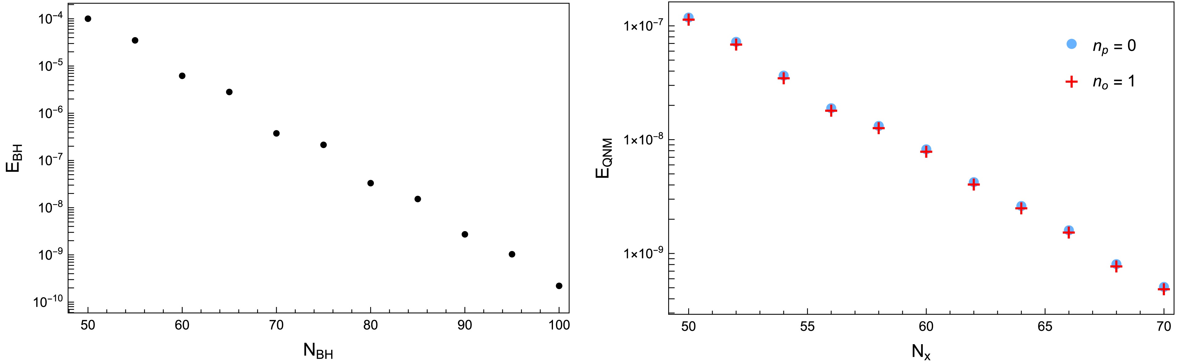
Figure A1. (color online) Residual convergence for
$ \alpha=\alpha_{\mathrm{EP}}\simeq0.79040751953125 $ and$ q=q_{\mathrm{EP}}\simeq1.0421911480 $ . Left: Maximum residual$ E_{\mathrm{BH}} $ of the background equations as$ N_{\mathrm{BH}} $ increases. Right: Maximum residual$ E_{\mathrm{QNM}} $ of the QNM equation as$ N_x $ increases for the$ n_p=0 $ and$ n_o=1 $ modes. Both residuals decrease approximately exponentially with increasing spectral resolution.We further examine the resolution dependence of the two modes involved in the near-coalescence. As shown in the left panel of Fig. A2, the
$ L^2 $ difference between the normalized radial wave functions of the$ n_p=0 $ and$ n_o=1 $ modes decreases rapidly as$ N_x $ increases. This indicates that the two eigenfunctions approach each other with increasing spectral resolution. For each mode, we also define the frequency difference relative to the corresponding result at$ N_x=70 $ as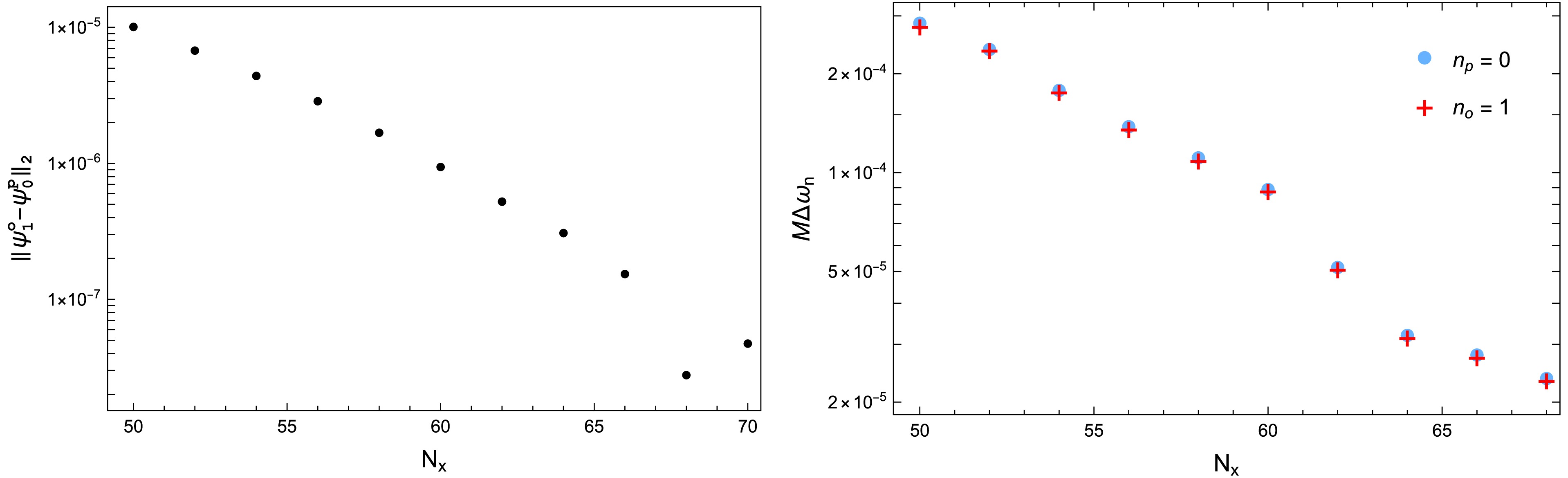
Figure A2. (color online) Resolution dependence of the two QNMs involved in the near coalescence, evaluated at
$ \alpha=\alpha_{\mathrm{EP}}\simeq $ $ 0.79040751953125 $ and$ q=q_{\mathrm{EP}}\simeq1.0421911480 $ . Left:$ L^2 $ difference between the normalized radial wave functions of the$ n_p=0 $ and$ n_o=1 $ modes. Right: Frequency difference$ \Delta\omega_n $ for each mode relative to its corresponding$ N_x=70 $ result. The wave-function difference decreases rapidly as$ N_x $ increases, while the frequency differences relative to the$ N_x=70 $ results decrease approximately exponentially.$ \Delta\omega_n(N_x) \equiv \left|\omega_n(N_x)-\omega_n(70)\right|. $
(A1) As shown in the right panel,
$ \Delta\omega_n $ decreases approximately exponentially as$ N_x $ increases, demonstrating the numerical stabilization of both QNM frequencies.These convergence tests are performed at the parameter point quoted in the main text and do not include a separate determination of
$ \alpha_{\mathrm{EP}} $ and$ q_{\mathrm{EP}} $ . Locating the EP requires an independent two-dimensional scan, whose numerical accuracy depends not only on$ N_x $ but also on the numerical precision of the parameter search and the coalescence criterion. Variations in the resulting EP coordinates would therefore not isolate the dependence on$ N_x $ alone. Instead, we keep the quoted parameter point fixed and directly test the convergence of the background solution, the two QNM solutions, and their eigenfunction coalescence as the spectral resolution increases. The quoted values of$ \alpha_{\mathrm{EP}} $ and$ q_{\mathrm{EP}} $ should therefore be understood as specifying the parameter point used throughout our numerical analysis, rather than as EP coordinates converged to all displayed digits. -
The background BH solution and QNM calculations use separate Chebyshev collocation grids, with resolutions denoted by
$ N_{\mathrm{BH}} $ and$ N_x $ , respectively. All calculations are performed using 50-digit working precision. The results reported in the main text use$ N_{\mathrm{BH}}=100 $ for the background solution and$ N_x=70 $ for the QNM problem.We perform the convergence tests at
$ \alpha=\alpha_{\mathrm{EP}}\simeq $ 0.79040751953125 and$ q=q_{\mathrm{EP}}\simeq1.0421911480 $ . For a numerical solution obtained with resolution$ N_{\mathrm{BH}} $ or$ N_x $ , we define$ E_{\mathrm{BH}} $ as the maximum absolute residual among the background field equations and$ E_{\mathrm{QNM}} $ as the maximum absolute residual of the radial QNM equation. These residuals are evaluated on uniform radial grids containing$ N_{\mathrm{BH}} $ and$ N_x $ points, respectively. As shown in Fig. 9, both residuals decrease approximately exponentially as the resolution increases and reach values of order$ 10^{-10} $ at the resolutions used in the main text.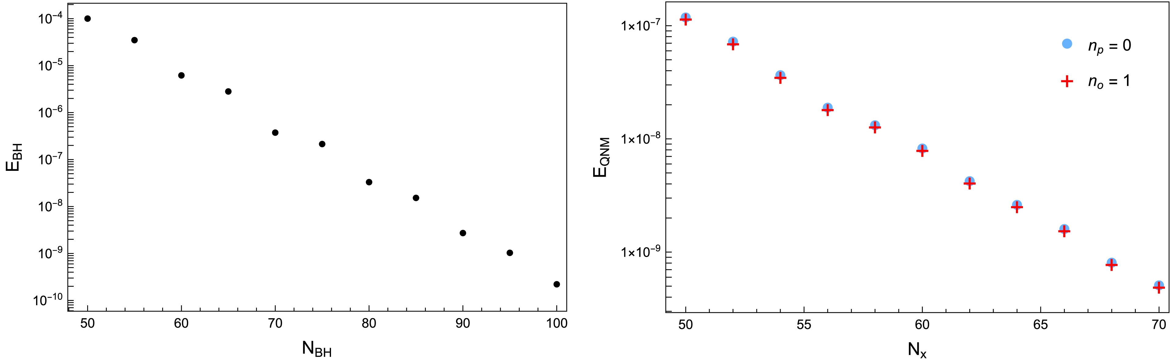
Figure 9. (color online) Residual convergence for
$ \alpha=\alpha_{\mathrm{EP}}\simeq0.79040751953125 $ and$ q=q_{\mathrm{EP}}\simeq1.0421911480 $ . Left: Maximum residual$ E_{\mathrm{BH}} $ of the background equations as$ N_{\mathrm{BH}} $ increases. Right: Maximum residual$ E_{\mathrm{QNM}} $ of the QNM equation as$ N_x $ increases for the$ n_p=0 $ and$ n_o=1 $ modes. Both residuals decrease approximately exponentially with increasing spectral resolution.We further examine the resolution dependence of the two modes involved in the near-coalescence. As shown in the left panel of Fig. 10, the
$ L^2 $ difference between the normalized radial wave functions of the$ n_p=0 $ and$ n_o=1 $ modes decreases rapidly as$ N_x $ increases. This indicates that the two eigenfunctions approach each other with increasing spectral resolution. For each mode, we also define the frequency difference relative to the corresponding result at$ N_x=70 $ as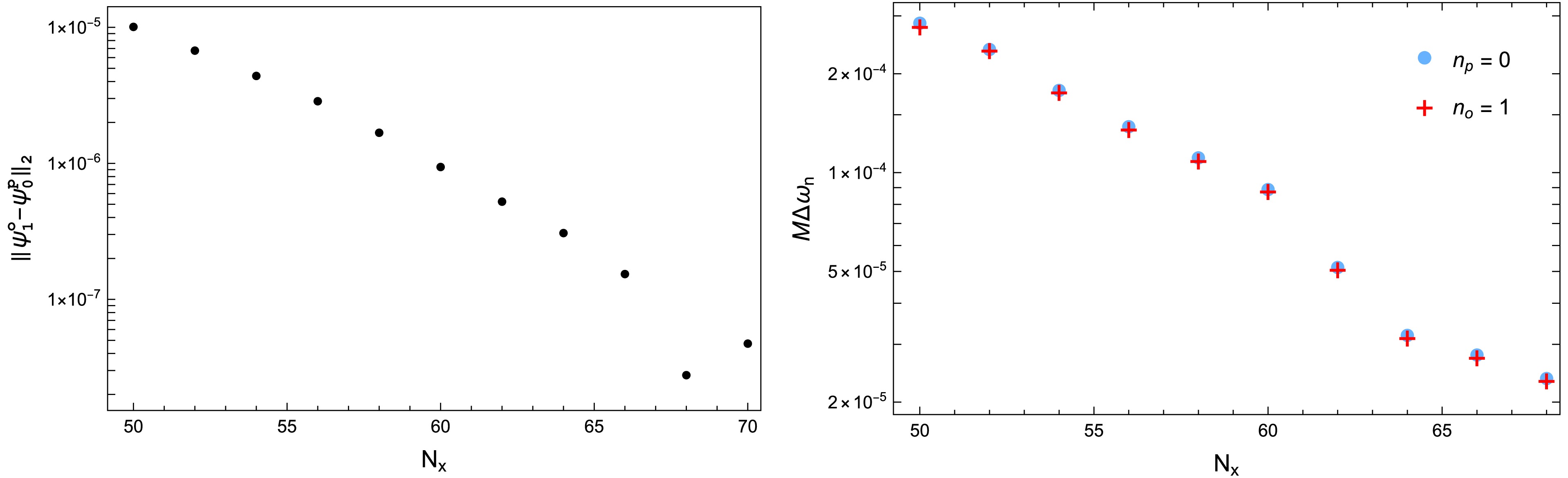
Figure 10. (color online) Resolution dependence of the two QNMs involved in the near coalescence, evaluated at
$ \alpha=\alpha_{\mathrm{EP}}\simeq0.79040751953125 $ and$ q=q_{\mathrm{EP}}\simeq1.0421911480 $ . Left:$ L^2 $ difference between the normalized radial wave functions of the$ n_p=0 $ and$ n_o=1 $ modes. Right: Frequency difference$ \Delta\omega_n $ for each mode relative to its corresponding$ N_x=70 $ result. The wave-function difference decreases rapidly as$ N_x $ increases, while the frequency differences relative to the$ N_x=70 $ results decrease approximately exponentially.$ \Delta\omega_n(N_x) \equiv \left|\omega_n(N_x)-\omega_n(70)\right|. $
(19) As shown in the right panel,
$ \Delta\omega_n $ decreases approximately exponentially as$ N_x $ increases, demonstrating the numerical stabilization of both QNM frequencies.These convergence tests are performed at the parameter point quoted in the main text and do not include a separate determination of
$ \alpha_{\mathrm{EP}} $ and$ q_{\mathrm{EP}} $ . Locating the EP requires an independent two-dimensional scan, whose numerical accuracy depends not only on$ N_x $ but also on the numerical precision of the parameter search and the coalescence criterion. Variations in the resulting EP coordinates would therefore not isolate the dependence on$ N_x $ alone. Instead, we keep the quoted parameter point fixed and directly test the convergence of the background solution, the two QNM solutions, and their eigenfunction coalescence as the spectral resolution increases. The quoted values of$ \alpha_{\mathrm{EP}} $ and$ q_{\mathrm{EP}} $ should therefore be understood as specifying the parameter point used throughout our numerical analysis, rather than as EP coordinates converged to all displayed digits.
Exceptional points in quasinormal spectra of hairy black holes
- Received Date: 2026-06-24
- Available Online: 2027-02-15
Abstract: Exceptional points (EPs) in quasinormal mode (QNM) spectra are non-Hermitian degeneracies at which both eigenvalues and eigenfunctions coalesce. In this paper, we identify an EP in the scalar QNM spectrum of hairy black holes in the Einstein-Maxwell-scalar theory by scanning the parameter space. We then investigate its implications for ringdown signals by extracting QNMs from time-domain waveforms. Our results show that an EP ansatz, which includes a resonant contribution containing a term linear in time, provides a more robust description of the ringdown at the EP than the standard ansatz based on a superposition of independent damped modes. In particular, it captures the resonant contribution associated with spectral coalescence more naturally. Moreover, even when the waveform is fitted with the standard ansatz, the resulting fit may still exhibit characteristic features of the EP ansatz.



 DownLoad: