Digital Quantum Simulation of Nonequilibrium Dynamics in the Schwinger Model under a Strong External Electric Field

Vacuum instability in strong-field quantum electrodynamics is a central problem in nonperturbative quantum field theory. In a sufficiently strong electric field, the quantum vacuum can decay via tunneling, producing particle–antiparticle pairs, a process known as the Schwinger effect [1−5]. This process exhibits a characteristic nonperturbative exponential dependence and is intrinsically a real-time nonequilibrium phenomenon [3, 6−8]. It is therefore difficult to describe reliably using traditional perturbation theory. Numerical methods that directly track the real-time evolution of quantum states are essential for understanding vacuum structure, pair production, and energy-transfer mechanisms in strong-field QED [9−12].

Lattice gauge theory provides a first-principles framework for studying nonperturbative quantum field theory [13−17]. In Euclidean path-integral Monte Carlo simulations, efficient importance sampling is possible when the weight can be interpreted as a nonnegative probability distribution. However, when the weight becomes complex, nonpositive, or highly oscillatory due to a chemical potential, a topological term, a fermion determinant, or a real-time phase factor, severe cancellations occur among different field configurations, and the statistical error grows rapidly with the system volume or the evolution time. This difficulty is usually referred to as the sign problem [18−20]. The Hamiltonian formalism is not by itself a source of quantum speedup, but it does not rely on Euclidean probability-weight sampling and can therefore bypass this class of sign problems associated with nonpositive sampling weights. The corresponding difficulty is then shifted to the direct treatment of an exponentially large Hilbert space. Quantum computation and quantum simulation provide natural platforms for real-time lattice field theory, since quantum many-body states and unitary time evolution can be directly represented with qubits [21−24].

The Schwinger model, namely quantum electrodynamics in 1+1 dimensions, is a standard low-dimensional model for studying strong-field nonequilibrium dynamics [25, 26]. Although it is much simpler than QED in 3+1 dimensions, it retains several essential features, including local U(1) gauge invariance, charge screening, confinement, chiral condensation, and vacuum instability [9, 10, 27−36]. In addition, gauge fields in one spatial dimension have no independent degrees of freedom. Under open boundary conditions, Gauss's law allows the electric field on each link to be expressed as a function of the matter charge distribution and the boundary electric field, thereby reducing the model to a purely fermionic Hamiltonian or, after a Jordan–Wigner transformation, a qubit Hamiltonian [29, 30, 37−39]. This feature makes the Schwinger model a useful benchmark platform for digital quantum simulation of lattice theories [40−48].

In recent years, the Schwinger model has become an important testbed for quantum simulations in high-energy physics. The real-time dynamics, pair production, thermalization, phase structure, and finite-temperature properties of the Schwinger model and related lattice models have been studied using platforms such as trapped ions, superconducting qubits, tensor networks, and cold atoms [11, 12, 43, 44, 49−61]. Related analog and digital quantum-simulation studies have also investigated gauge invariance, thermalization, topological θ angles, confinement dynamics, scattering processes, and higher-dimensional gauge-theory dynamics [62−72]. In particular, quenches in which an external electric field is suddenly switched on have been used to investigate strong-field-induced particle–antiparticle production and vacuum response [9, 11, 12]. In related studies, the zero-field ground state is often prepared using VQE, evolved under the Hamiltonian with an external field, and compared with results from exact diagonalization or tensor-network calculations [9, 12, 73−76].

In this work, we study the lattice Schwinger model with a constant external electric field and focus on the finite-size nonequilibrium dynamics after an electric-field quench. We first construct the lattice Hamiltonian under open boundary conditions and map it to a Pauli-operator form using the Jordan–Wigner transformation. We then use VQE to prepare the zero-field vacuum state, which is taken as the initial state when the external field is switched on. The real-time evolution is implemented using a second-order Trotter–Suzuki decomposition. In contrast to approaches based on the McLachlan variational principle and fixed-depth variational real-time evolution, the present work uses explicit digital Trotter evolution and examines the total charge, total energy, spatial-point charge distribution, vacuum-state fidelity, and electric-field energy [11, 12, 77−81]. By comparing these quantities with ED results, we assess the reliability of the protocol for describing strong-field dynamics in finite lattice systems. The numerical implementation is based on the Qiskit quantum computing framework [82, 83]. We also perform scans over the external field and analyze the chiral condensate, the low-energy levels, and the finite-size critical external field.

The paper is organized as follows. Section II introduces the lattice Schwinger model with an external electric field, the Gauss-law reduction, and the qubit encoding. Section III describes the VQE state preparation and the second-order Trotter–Suzuki evolution. Section IV presents numerical results. Section V summarizes the work and discusses possible extensions, including larger system sizes, improved ansatzes, and implementation on noisy quantum hardware. Appendix A provides dynamical checks for the $ N = 12 $.

In natural units, the continuum Lagrangian density of the Schwinger model is given by [25, 26, 28].

where $ D_{\mu} = \partial_{\mu} + igA_{\mu} $ is the covariant derivative, ψ is the fermion field, m is the bare fermion mass, g is the gauge coupling, and $ A_{\mu} $ is the $ U(1) $ gauge field. The field-strength tensor is defined as $ F_{\mu\nu} = \partial_{\mu}A_{\nu} - \partial_{\nu}A_{\mu} $. In $ 1+1 $ dimensions, the electric field is the only independent component of the field-strength tensor; we adopt the convention $ E \equiv F_{01} = \partial_{0}A_{1} - \partial_{1}A_{0} $. In the temporal gauge $ A_{0} = 0 $, this reduces to $ E = \partial_{0}A_{1} $. The Hamiltonian is

To simulate this theory with a finite number of qubits, the continuum field theory is discretized on a finite lattice using the Kogut–Susskind staggered-fermion formulation [14, 29, 30]. The continuum Dirac field is written as $ \psi(x)=(\psi_1(x),\psi_2(x))^T $, and its two spinor components are assigned to neighboring staggered lattice sites. The mapping is

Here, $ i=1,\ldots,N/2 $ labels the physical spatial points, each of which is represented by two neighboring staggered lattice sites. The fermionic degrees of freedom therefore reside on the lattice sites, whereas the gauge degrees of freedom reside on the links between neighboring sites.

Consider a system with N lattice sites and lattice spacing a, where the sites are labeled by $ n = 0,1,\ldots,N-1 $. The discretized Hamiltonian is

Here, $ \phi_{n} $ is the staggered-fermion operator at the n-th lattice site, $ U_n \equiv U_{n,n+1} $ is the gauge-link variable on the link connecting sites n and $ n+1 $, and $ L_{n} $ is the corresponding lattice electric field. The first term describes hopping between neighboring lattice sites; the second term is the staggered mass term; and the third term is the electric-field energy. Unless otherwise specified, all numerical calculations in this work are performed in lattice units with $ a = m = g $.

In $ 1 + 1 $ dimensions, the gauge field has no independent propagating degrees of freedom, and the electric field on each link is fully determined by Gauss's law and the boundary conditions. The lattice Gauss law is given in [14, 29, 30]

In this work, we impose open boundary conditions and set the electric field at the left boundary to a constant external field ε, with $ L_{-1}=\varepsilon $ [12, 28, 57, 60]. Iterating Gauss's law from the left boundary gives

Here, l denotes the summation index over lattice sites from the left boundary to site n.

Therefore, the external field ε is not introduced as an independent potential-energy term. Instead, it enters the Hamiltonian through the link and the corresponding electric-field energy [12, 28, 57]. It modifies the background electric-field configuration and thereby affects both the ground-state structure and the real-time dynamics.

A further gauge transformation can absorb the link variable $ U_{n} $ into the hopping term [12, 29, 30, 57]. The Hamiltonian can then be written in a purely fermionic form as

This expression shows that, once the gauge field is eliminated, the electric-field energy becomes a long-range interaction induced by the charge distribution. The external field ε, together with the lattice charge distribution, determines the electric field on each link and is a key ingredient in the strong-field dynamics studied in this work.

To implement the model described above for digital quantum simulation, the fermionic operators must be mapped to Pauli operators. In this work, we employ the Jordan-Wigner transformation [37−39],

After the Jordan-Wigner mapping, the lattice Schwinger model can be expressed as a Pauli Hamiltonian

where the kinetic term is

the mass term is

and the electric-field energy term is

Since $ H_{E} $ contains the cumulative charge from the left boundary up to the n-th lattice site, it generates long-range interactions in the Pauli representation. This nonlocal structure is a direct consequence of eliminating the gauge degrees of freedom in one spatial dimension, and it distinguishes the present model from ordinary nearest-neighbor spin chains [12, 29, 30, 57].

To characterize the nonequilibrium dynamics under a strong external electric field, we focus primarily on the following observables.

The total charge operator is defined as

The total charge is a conserved quantity associated with the $ U(1) $ gauge symmetry [11, 12, 53]. In real-time evolution, total-charge conservation provides a basic check of the correctness of the initial state, the Gauss-law constraint, and the time-evolution algorithm.

The local charge density at the n-th lattice site is

To display the physical charge distribution more clearly, we also measure the local charge density at each spatial point, defined as the sum of the charge densities at neighboring staggered lattice sites. For each spatial point i, the spatial-point charge is then defined

This observable is used to characterize the spatial separation between positive and negative charges induced by the external electric field.

The corresponding total electric-field energy is evaluated as the expectation value of the electric-field-energy operator in Eq.(12)

Here, $ \langle\cdots\rangle_t $ denotes the expectation value in the time-evolved state $ |\psi(t)\rangle $.

To quantify the stability of the initial vacuum state under the external field, we define the vacuum-state fidelity as [3, 9, 12, 49]

where $ \psi_{0} $ is the zero-field ground state and $ \psi(t) $ is the state evolved following the electric-field quench.

For the static scan over the external field, we also introduce the chiral condensate density [9, 10, 27, 28, 31−36, 59, 60],

which identifies field-induced ground-state reconstruction in finite-size systems.

For a given system size N, lattice spacing a, fermion mass m, gauge coupling g, and external-field strength ε, we construct the sparse-matrix Hamiltonian of the lattice Schwinger model and use exact diagonalization (ED) to obtain the ground state, the low-energy spectrum, and benchmark real-time dynamics. These results are used to assess the accuracy of the quantum algorithms.

The initial state for real-time evolution is taken to be the ground state of the zero-field Hamiltonian $ H_{\varepsilon = 0} $. In this work, we use the variational quantum eigensolver (VQE) to prepare this initial vacuum state [73−76]. For a trial state $ \psi(\theta) $ generated by a parameterized quantum circuit, where $ \theta=(\theta_1,\theta_2,\ldots) $ denotes the set of variational circuit parameters, VQE approximates the ground-state energy and wave function by minimizing the expectation value of energy

We employ the hardware-efficient RealAmplitudes parameterized circuit and use the Sequential Least Squares Programming (SLSQP) algorithm as the classical optimizer [75, 82, 83]. To mitigate the influence of local minima, multiple restarts with random initial parameters are used during optimization [84]. The accuracy of the VQE-prepared initial state is evaluated by comparing the ground-state energy and wave-function fidelity with the ED results. In addition to the zero-field initial-state preparation, VQE is also used in the static external-field scan to estimate the ground-state energy $ E_{0}(\varepsilon) $ and the corresponding chiral condensate at different external-field strengths.

To further compare the low-energy structure, the first excited-state energy is estimated using the variational quantum deflation (VQD) method with an orthogonality penalty [85]. After obtaining the approximate VQE ground state $ \psi_{0}^{VQE} $, the variational objective function for the first excited state is

where β denotes the orthogonality-penalty coefficient. The second term suppresses the overlap between the candidate state and the VQE ground state, thereby driving the optimization toward the first-excited-state subspace. After optimization, the first-excited-state energy is evaluated as

Its accuracy is assessed by comparison with the ED result $ E_{1}^{ED} $. In the external-field scan, the optimized parameters from the previous field point are used as the initial parameters for the next field point to improve optimization stability. Thus, the quantum-algorithm results in the static external-field scan consist of two parts: VQE provides the ground-state energy and the chiral condensate, while VQD provides the first excited-state energy.

After obtaining the zero-field ground state, we study the real-time dynamics following the sudden switch-on of the external electric field. The initial state is taken as the ground state at $ \varepsilon = 0 $. After the quench, the system evolves under the Hamiltonian $ H_\epsilon $

Because the Hamiltonian is decomposed into several noncommuting terms, the full time-evolution operator cannot be implemented directly [77−81]. If the total Hamiltonian is expressed as a sum of L terms, $ H = \sum\nolimits_{j = 1}^{L}H_{j} $, and the total evolution time T is divided into r time steps, the second-order Trotter-Suzuki decomposition is

where $ \Delta t = T/r $. The local error per time step is $ O\left( \Delta t^{3} \right) $, and the global error is second order in $ \Delta t $ for a fixed total evolution time. Compared with the first-order decomposition, the symmetric second-order formula provides higher accuracy for the same time step, at the cost of an increased circuit depth [77−81].

In the numerical implementation, the full Pauli Hamiltonian is passed to a second-order Suzuki–Trotter synthesizer, and Suzuki–Trotter (order=2, reps=1) is used to generate the evolution circuit for a single time step. The primary time step is chosen as $ \Delta t = 0.1 $, and the total evolution time is taken in the range $ T/a \in [0,12] $. A time-step convergence check using $ \Delta t=0.2 $, $ 0.1 $, and $ 0.05 $ confirms the expected second-order convergence and shows that $ \Delta t=0.1 $ provides sufficient accuracy for the dynamical observables considered here. The representative external-field strengths in the dynamical calculations are selected according to the observable under consideration. In particular, the spatial-point charge distribution and electric-field energy response are studied primarily for $ \varepsilon = 0.5,1.0,1.5,2.0 $, while the analysis of the vacuum-state fidelity and the effective decay rate is further extended to stronger external fields. The numerical implementation is based on Qiskit and standard scientific Python packages [82, 83, 86−88]. The present simulations are performed on classical computers and do not account for quantum errors. In the present encoding, the circuit width is equal to the lattice size N. For the two-layer RealAmplitudes ansatz used in most dynamical calculations, the circuit depths are 24 and 36 for $ N=8 $ and $ N=12 $, respectively. After decomposition into elementary one- and two-qubit gates, the depths of a single second-order Suzuki–Trotter step are approximately 287 and 455, respectively, and the total real-time evolution depth increases linearly with the number of Trotter steps.

The main results are summarized as follows. For the system with $ N = 8 $ and $ a = m = g = 1 $, VQE prepares the ground state with high accuracy. We scan over the external field strength and calculate the chiral condensate and energy gap. These features are consistent with the flip of the finite-volume ground state. We then investigate the electric-field quench of the zero-field ground state. The second-order Trotter-Suzuki evolution preserves the total charge and total energy, and it shows good agreement with the ED results. The external electric field drives oscillations of the spatial point charges near the open boundaries. The vacuum-state fidelity exhibits an effective exponential decay within the early-time window, while the electric-field energy shows quasiperiodic behavior, reflecting finite-size energy redistribution between the electric-field energy and the fermion sectors.

We first examine the VQE preparation of the zero-field ground state for $ N = 8 $, $ a = m = g = 1 $, and $ \varepsilon = 0 $. The results are shown in Table I. The fidelity is defined as $ F=|\langle\psi_{0}^{\mathrm{ED}}|\psi_{0}^{\mathrm{VQE}}\rangle|^{2} $. These results indicate that the chosen parameterized circuit can approximate the zero-field ground state with high accuracy at the present system size, providing a reliable initial state for the subsequent electric-field-quench dynamics.

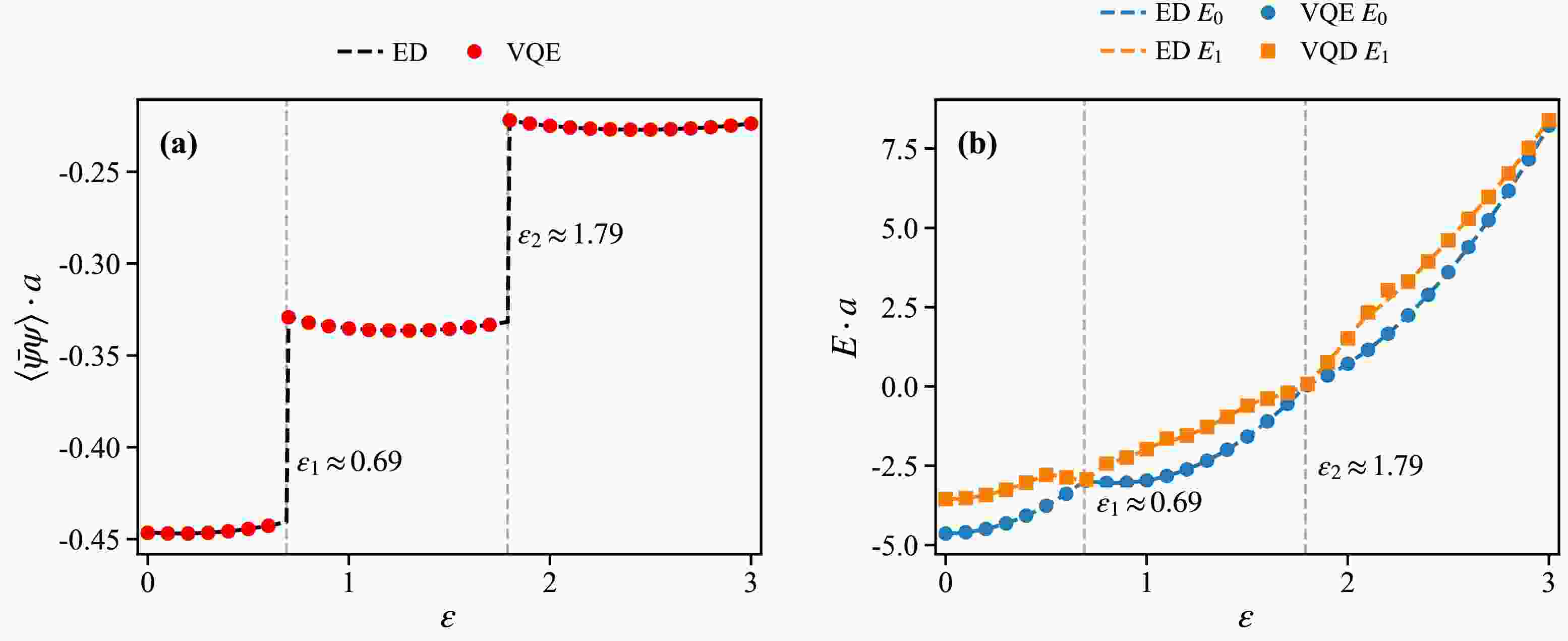
We then turn on the external field and prepare the ground and first excited states. We calculate the chiral condensate $ \langle\bar\psi\psi\rangle $ of the ground state, as shown in Figure 1(a), and the ground state energy $ E_0 $ and the first excited state energy $ E_1 $, as shown in Figure 1(b).

Figure 1.  Static observables as functions of the external-field strength ε. The left figure shows the chiral condensate of the ground state, while the right figure shows the energies of the ground state and the first excited state

The chiral condensate closely resembles a step function, with jumps occurring when the energy gap between the ground state and the first excited state vanishes. This result indicates that the external electric field can modify the vacuum structure of the finite system, driving the ground state from one to another. This phenomenon corresponds to a first-order phase transition at zero temperature, as observed in various studies of 1+1D models [28, 32, 59]. The VQE results are in overall agreement with the ED ones.

We emphasize that the external-field scan discussed here is performed in finite-size systems; consequently, the location of the low-energy spectral reconstruction depends on the system size. For each lattice size N, we define the energy gap as $ \Delta(\varepsilon,N)=E_1(\varepsilon,N)-E_0(\varepsilon,N) $, and denote by $ \varepsilon_c(N) $ the lowest positive external-field strength ε at which $ \Delta(\varepsilon,N) = 0 $. As a simple estimate, we adopt the following picture: for $ \varepsilon \lt \varepsilon_c $, the ground state has a trivial particle distribution, whereas the first excited state has an antiparticle at the left boundary that screens the external field. In this configuration, the antiparticle corresponds to a local charge $ q_1=-1 $ on the odd staggered site $ n=1 $; according to Gauss's law, $ L_0 $ remains equal to ε, whereas the remaining $ N-2 $ internal links, $ L_1,\ldots,L_{N-2} $, are shifted from ε to $ \varepsilon-1 $. The energy gap then arises mainly from the mass of the particles and the difference in the electric field energy, $ \Delta(\varepsilon,N)\approx \dfrac{1}{2}(N-2)(\varepsilon-1)^2 + m-\dfrac{1}{2}(N-2)\varepsilon^2=\dfrac{1}{2}(N-2)(1-2\varepsilon)+m $. Thus, the critical field is $ \varepsilon_c(N)\approx \dfrac{m}{(N-2)}+\dfrac{1}{2} $. We plot $ \varepsilon_c(N) $ as a function of $ 1/(N-2) $ in Figure 2. The data exhibit an approximately linear dependence on this variable, and linear extrapolation gives $ \varepsilon_c(\infty)\approx0.496 $. The infinite-size value $ \dfrac{1}{2} $ can also be derived from Coleman's analysis of the massive Schwinger model: $ \theta=\pi $ is the special point associated with the first-order transition [28]. In the equivalent background-field description, $ \varepsilon=\theta/(2\pi) $. Therefore, the Coleman point $ \theta=\pi $ corresponds to the theoretical reference value $ \varepsilon= \dfrac{1}{2} $.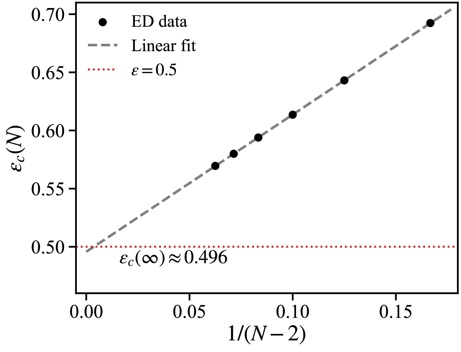

Figure 2.  Finite-size critical field $ \varepsilon_c(N) $ as a function of the boundary-shifted inverse size $ 1/(N-2) $.

We now turn to the main part of this work. We prepare the ground state in the absence of an external field, then turn the field on at $ t=0 $ and study the time evolution of the state.

First, we test the conservation laws after the electric-field quench. For different external-field strengths, the total charge $ Q_N(t) $ remains extremely close to zero throughout the time evolution. This indicates that the second-order Trotter-Suzuki evolution preserves the $ U(1) $ charge, as expected.

We also calculate the total energy shift, $ \Delta E(t) = E(t) - E(0) $. $ \Delta E(t) $ remains very close to zero throughout the simulated time interval. This shows that, with the chosen time step, the time evolution is numerically stable. The results are shown in Figure 3.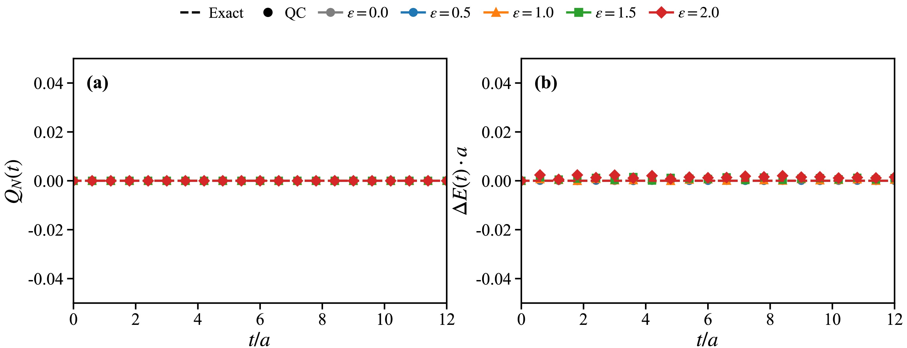

Figure 3.  Time evolution of the total charge $ Q_N(t) $ (left) and the total energy shift $ \Delta E(t) = E(t) - E(0) $ (right). In both panels, dashed lines denote ED results, while dots denote the results obtained from the quantum algorithm.

Although the total charge is conserved, the spatial charge distribution $ Q_i(t) $ undergoes a pronounced rearrangement, as displayed in Figure 4. After the field quench, a charge-anticharge pair is periodically produced and annihilated at the boundary of the system. The period and amplitude of the oscillation increase with the external field strength. The response is strongly enhanced near the open boundaries, whereas $ Q_2(t) $ and $ Q_3(t) $ exhibit only weaker oscillations around zero. This behavior can be understood as the screening effect: a pair of charges at the boundary provides more effective screening of the external background field. As a related quantity, we also calculate the time evolution of the total electric-field energy $ H_E(t) $ for different ε, as shown in Figure 5. When the charge pair is produced, energy is transferred from the electric field to the fermions, and when it is annihilated, the energy returns to the field. However, $ H_E(t) $ does not exhibit as simple a periodic pattern as $ Q_i(t) $.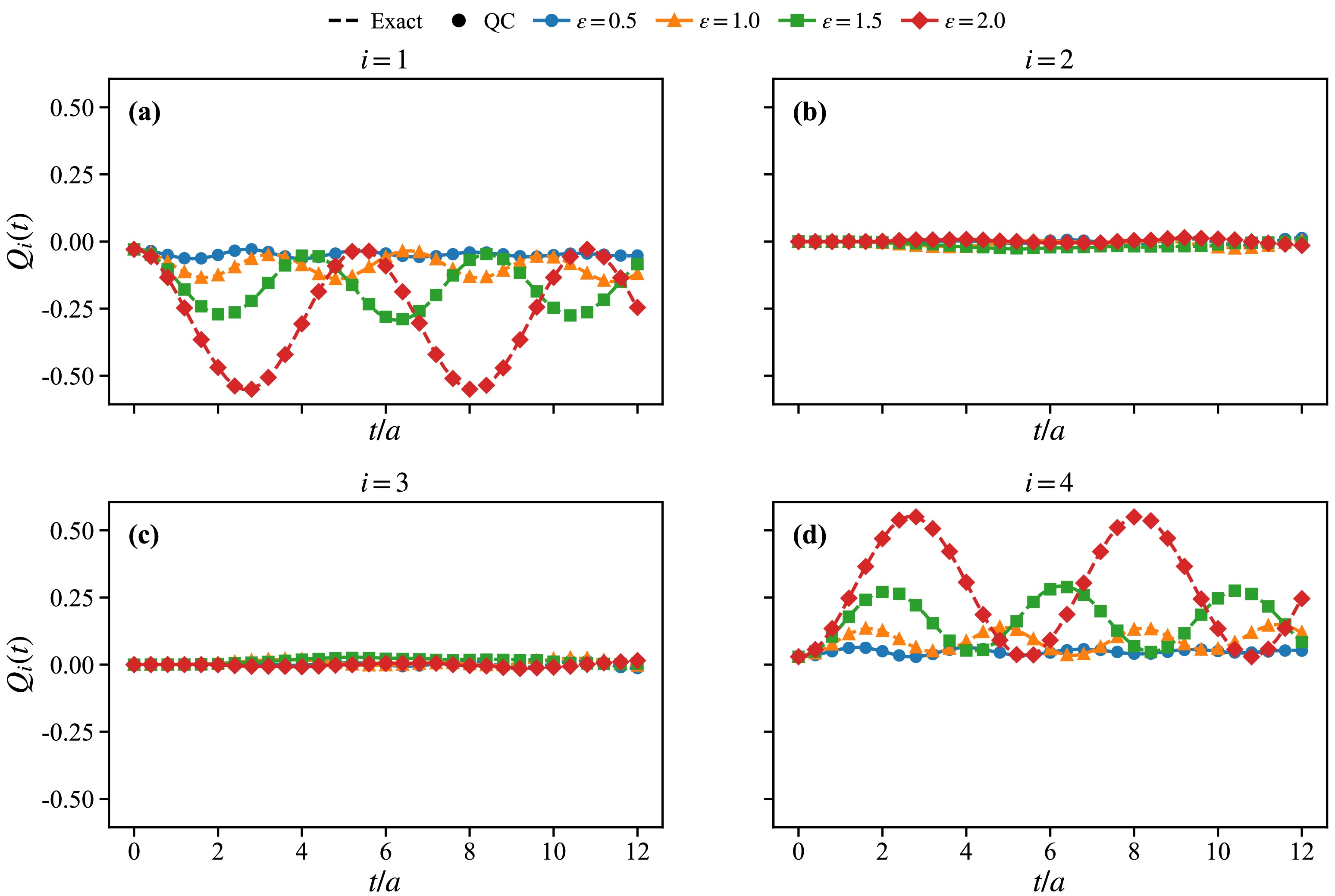

Figure 4.  Time Evolution of the Spatial Charge

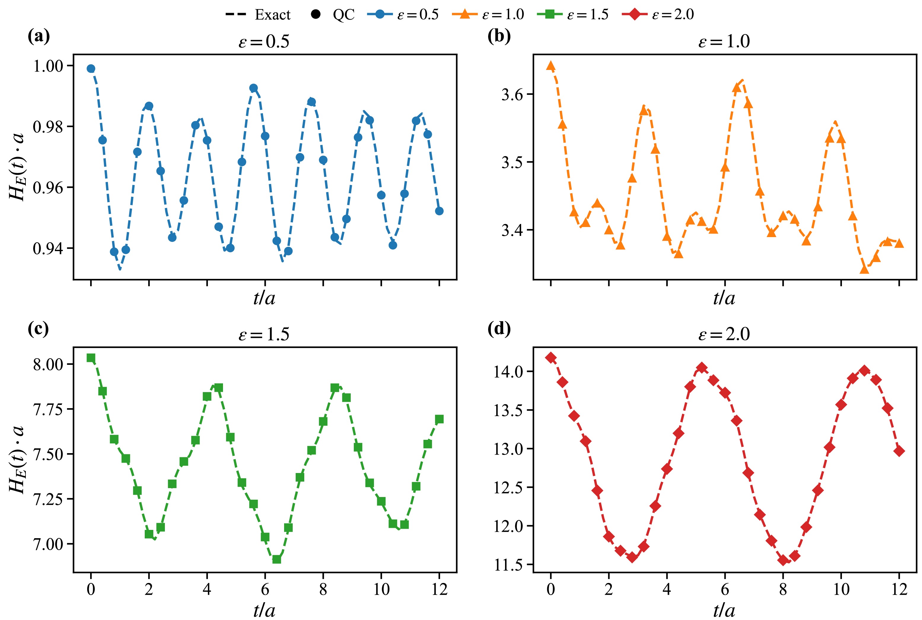
Figure 5.  Time evolution of the total electric-field energy $ H_{E}(t) $ under different external-field strengths.

In the staggered-fermion description, the charge at a given physical spatial point is obtained by combining two neighboring staggered-site contributions as $ Q_i(t)=q_{2i-2}(t)+ q_{2i-1}(t) $, with the corresponding site-resolved results shown in the Appendix. The electric-field energy $ H_E(t) $, on the other hand, is determined by the sum of the squares of the electric fields over the whole chain and therefore need not follow the same simple oscillation pattern as $ Q_i(t) $.

It is also notable that the dependence of the period and amplitude on ε appears smooth, unlike the step-like behavior of the static ground-state chiral condensate shown in Figure 1(a). This is not surprising, as Figure 1(b) shows that the dependence of the eigenenergies on ε is indeed smooth.

To characterize the system's rate of deviation from the initial state, we calculate the vacuum-state fidelity $ P_{\mathrm{vac}}(t) = \left| \langle\psi_{0} \right|\psi(t)\rangle|^{2} $. This quantity describes the probability that the system remains in the initial vacuum state under driving by the strong external electric field and serves to characterize the field-induced deviation from the

Figure 6 shows that, for weak external fields, the vacuum-state fidelity remains close to unity. As the external field increases, the system deviates more rapidly from the zero-field vacuum, indicating that a stronger external field enhances the nonequilibrium response of the system. Since the present study concerns a finite closed system, $ P_{\mathrm{vac}}(t) $ does not decay strictly monotonically; instead, it exhibits finite-size revivals and quasiperiodic oscillations similar to $ H_E $. Furthermore, the quantum algorithm results agree well with the ED results, demonstrating that the evolution protocol captures the vacuum response of the finite-lattice system.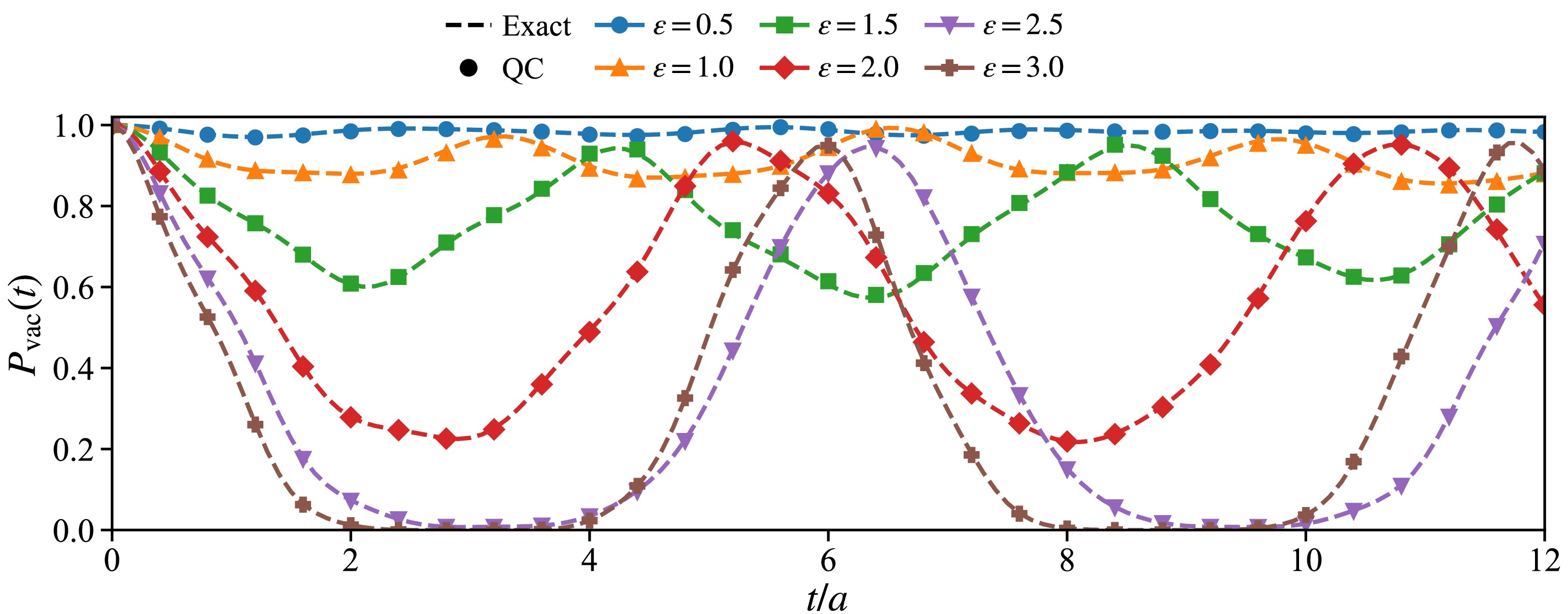

Figure 6.  Time evolution of vacuum-state fidelity under different external field strengths.

To further quantify the initial decrease of the vacuum-state fidelity under different external fields, we perform an effective exponential fit to $ P_{\mathrm{vac}}(t;\varepsilon) $ in the early-time window $ 0 \leq t/a \leq 1.0 $: $ P_{\mathrm{vac}}(t;\varepsilon) \simeq A(\varepsilon)\exp\left[ - \gamma_{\mathrm{eff}}(\varepsilon)t \right]. $ Equivalently, we fit $ -\ln P_{\mathrm{vac}}(t;\varepsilon) = \gamma_{\mathrm{eff}}(\varepsilon)t + c(\varepsilon) $ and define the slope $ \gamma_{\mathrm{eff}} $ as the effective decay rate. Within this early-time window, the numerical results show that $ -\ln P_{\mathrm{vac}}(t;\varepsilon) $ is approximately linear in time, indicating that the initial decrease of the vacuum-state fidelity can be characterized by an exponential form.

Figure 7 shows the dependence of $ \gamma_{\mathrm{eff}} $, extracted from the fitting procedure described above, on the external-field strength ε. The effective decay rate increases monotonically with ε, indicating that a stronger external field drives the system away from the initial vacuum state more rapidly.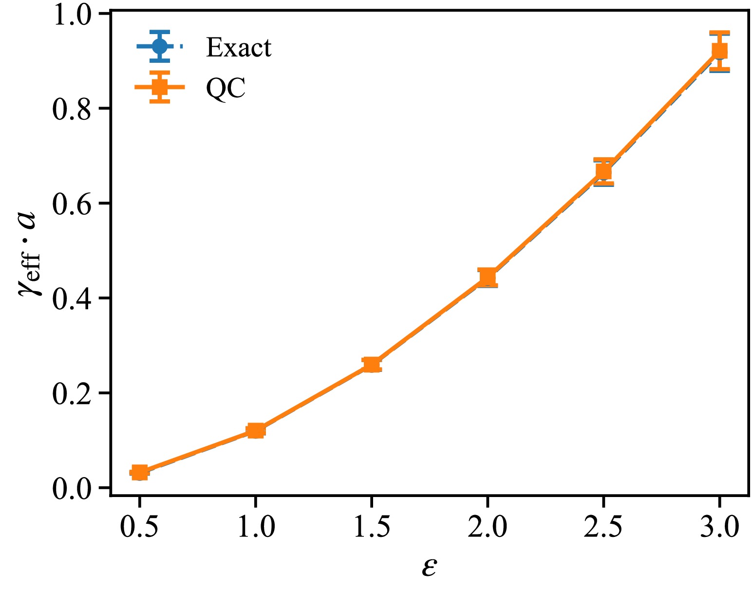

Figure 7.  The effective decay rate $ \gamma_{\mathrm{eff}} $ was obtained by fitting.

As a system-size check, Appendix A also presents dynamical comparison results for the $ N = 12 $ lattice system. Similar to the $ N = 8 $ case, the spatial charge distribution in the $ N = 12 $ system still exhibits boundary charge separation induced by the external electric field, indicating that this phenomenon is not a numerical artifact specific to the small $ N = 8 $ system. For the same external-field strength, $ P_{\mathrm{vac}}(t) $ in the $ N = 12 $ system is more sensitive to the external field and deviates from its initial value more rapidly. This may be related to the denser low-energy spectrum and the larger number of excited states participating in the quench dynamics in the larger systems.

In this work, we studied the static ground-state structure and nonequilibrium dynamics of the finite-lattice Schwinger model under a constant external electric field. We used VQE and VQD to compute the low-energy states and employed a second-order Trotter-Suzuki decomposition to simulate the real-time evolution after an electric-field quench. The results obtained from the quantum algorithms were compared with exact diagonalization throughout the calculations.

The external-field scan reveals step-like changes in the chiral condensate near the field strengths at which the ground and first excited states are closest in energy. The corresponding characteristic field strength exhibits a clear finite-size dependence. After the electric-field quench, the total charge and total energy remain approximately conserved. The system exhibits boundary charge separation, quasiperiodic electric-field-energy redistribution, and a field-dependent decrease in the vacuum-state fidelity. The site-resolved charge dynamics and the $ N=12 $ results further show that the main dynamical features persist on a larger lattice.

These results demonstrate that VQE-based state preparation combined with digital real-time evolution can reproduce the main static and dynamical responses of the finite-lattice Schwinger model. Future work may extend the present study to larger systems, improved variational ansatzes, noisy quantum hardware, and time-dependent fields.

The real-time dynamics in the main text focus primarily on the $ N=8 $ lattice and use the spatial-point charge $ Q_i(t) $ to illustrate the field-induced charge separation. In this appendix, we provide the corresponding site-resolved charge dynamics and a check for the $ N=12 $ lattice. The line and marker conventions are the same as those in the main text.

Figure 8 shows the time evolution of the staggered-site charge $ q_n(t) $ for the $ N=8 $ lattice. Compared with the spatial-point charge $ Q_i(t) $ in the main text, the site-resolved charge exhibits more detailed oscillations of the staggered component. The dominant response still appears near the open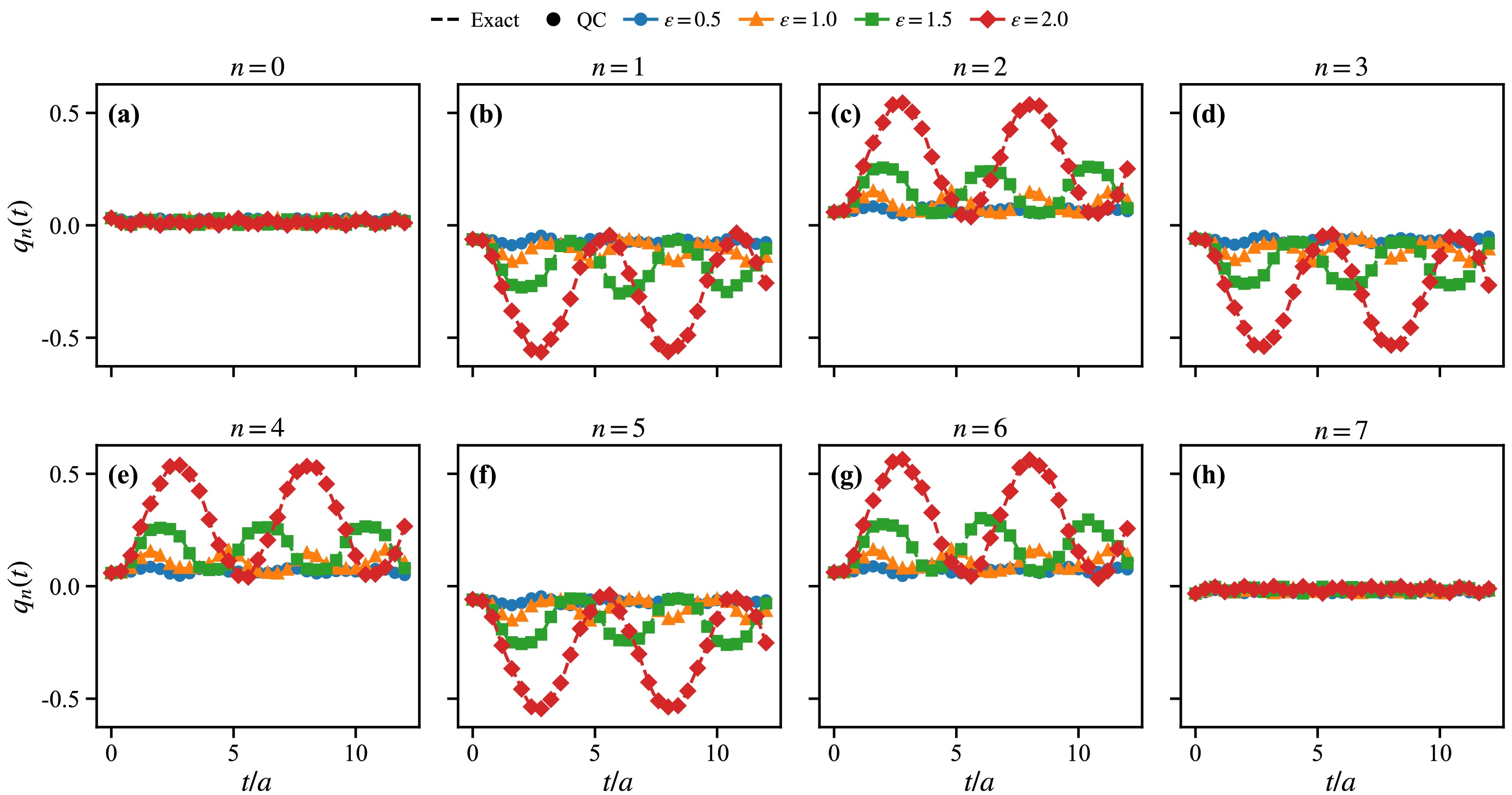

Figure 8.  Time evolution of the site-resolved charge $ q_n(t) $ for the $ N=8 $ lattice.

Figure 9 shows the corresponding site-resolved charge dynamics for the $ N=12 $ lattice. The larger system exhibits a greater number of local oscillatory components, while the boundary-dominated response remains similar to that of the $ N=8 $ case.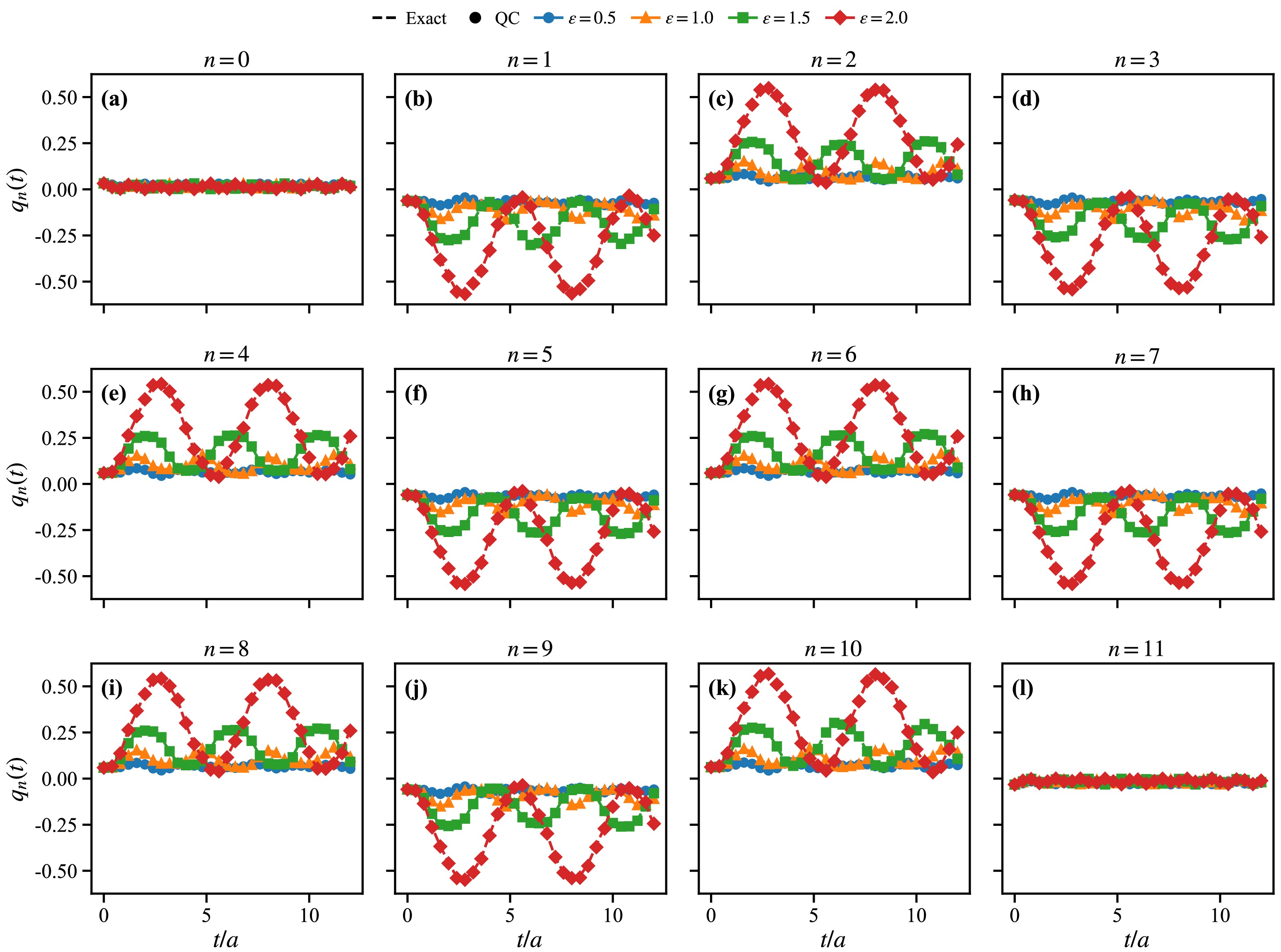

Figure 9.  Time evolution of the site-resolved charge $ q_n(t) $ for the $ N =12 $ lattice.

For comparison with the spatial-point observable used in the main text, Figure 10 shows $ Q_i(t) $ for the $ N=12 $ lattice. The result exhibits the same qualitative boundary charge separation as in the $ N=8 $ lattice.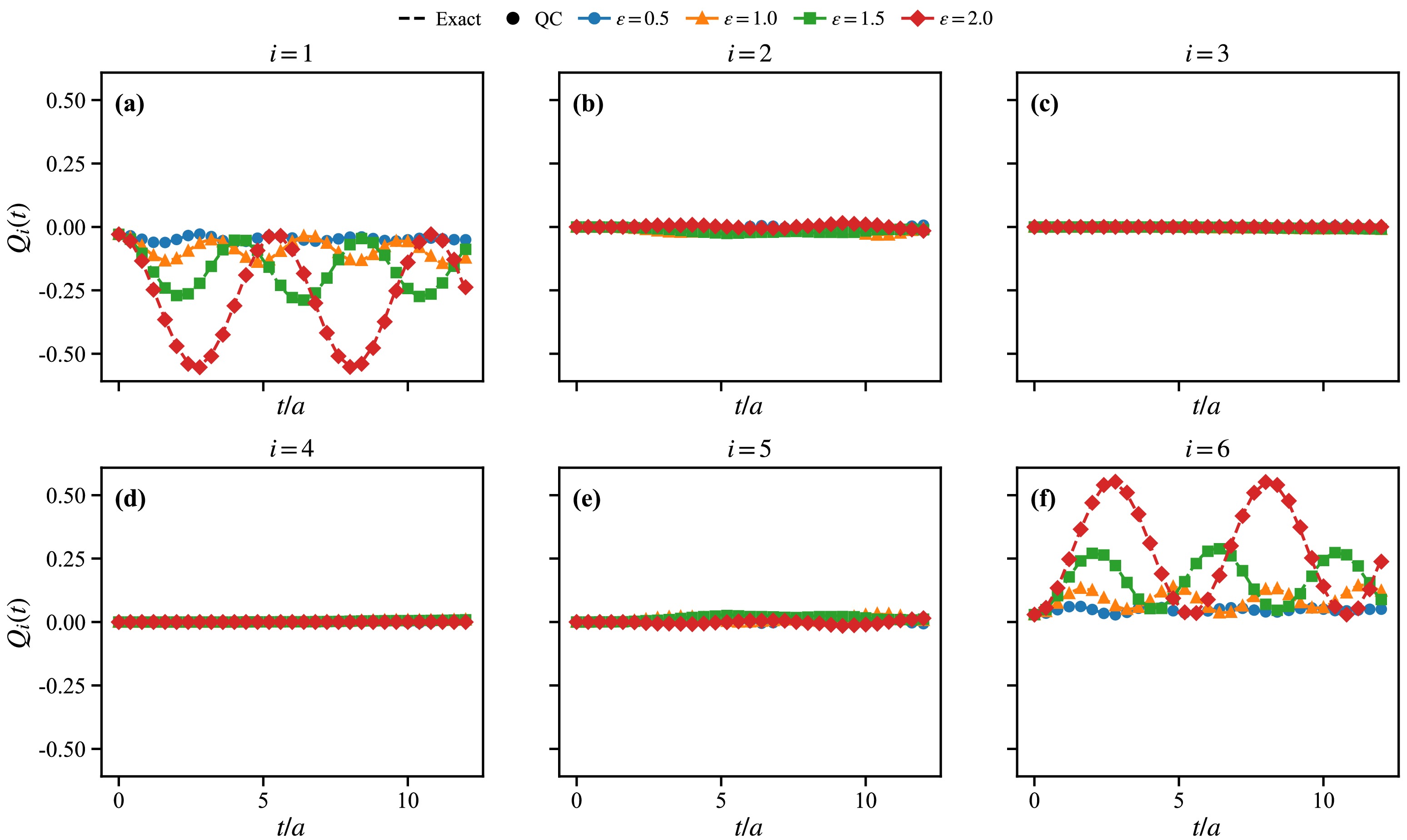

Figure 10.  Time evolution of the spatial point charge $ Q_i(t) $ in the $ N=12 $ lattice.

We also compare the vacuum-state fidelity for the $ N=12 $ lattice. As shown in Figure 11, under the same external-field strength, $ P_{\mathrm{vac}}(t) $ deviates from its initial value more rapidly than in the $ N=8 $ case. This behavior may be related to the denser low-energy spectrum and the larger number of excited states involved in the quench dynamics.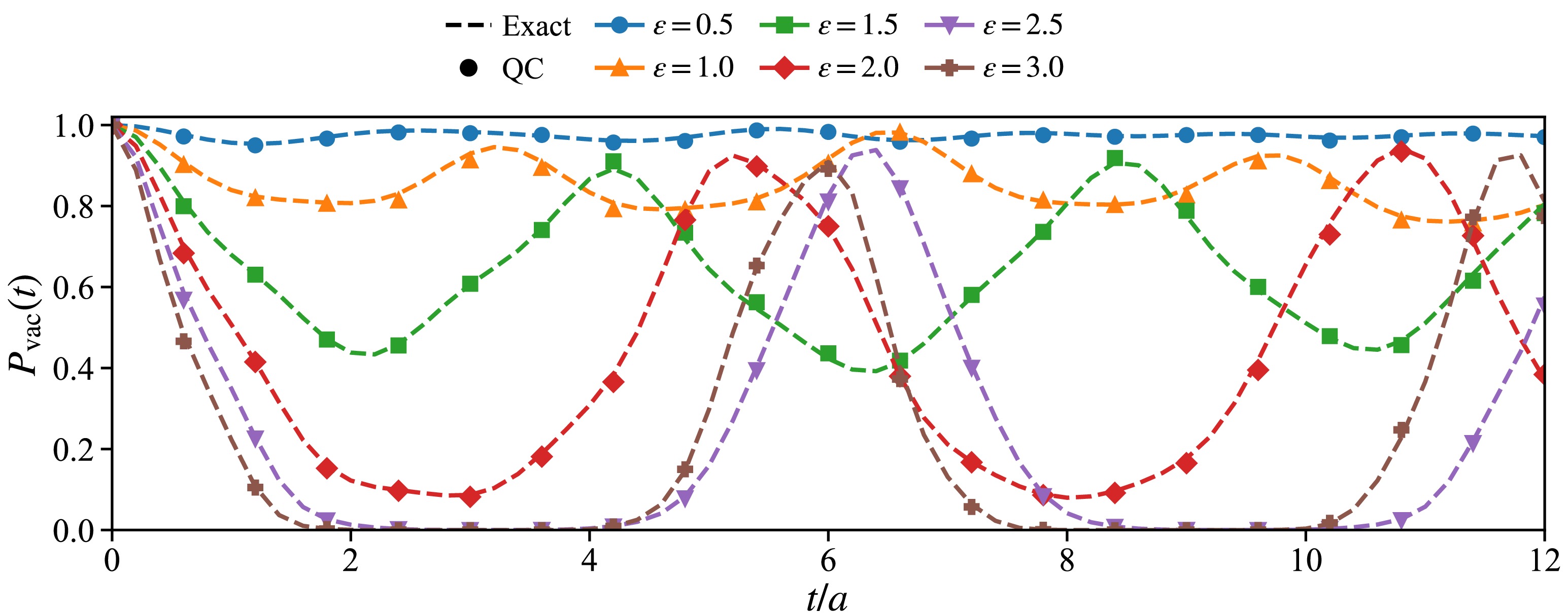

Figure 11.  Time evolution of the vacuum-state fidelity $ P_{\mathrm{vac}}(t) $ for the $ N=12 $ lattice

Overall, the $ N=8 $ and $ N=12 $ results show that both the boundary charge separation and the deviation from the initial vacuum state persist as the system size increases.