


 Abstract
 HTML
 Reference
 Related
 PDF



-
Extreme mass-ratio systems provide a natural setting in which the less massive body can be treated as a test object moving in a fixed gravitational background. A prominent example is the population of S-stars orbiting Sagittarius A*, for which increasingly precise astrometric measurements continue to sharpen constraints on the gravitational field at the Galactic Center [1, 2]. These developments motivate detailed studies of relativistic orbital dynamics, including departures from geodesic motion arising from intrinsic spin and electromagnetic interactions.
Gibbons and Maeda obtained static, spherically symmetric charged black-hole solutions in Einstein–Maxwell–dilaton gravity; independently, Garfinkle, Horowitz, and Strominger obtained analogous solutions in the context of low-energy string theory [3, 4]. These solutions form the basis of the geometry commonly called the GMGHS black hole. An important feature of the GMGHS solution is the distinction between its Einstein-frame and conformally related string-frame representations. This distinction is important for massive-particle dynamics because the conformal transformation preserves the null structure but generally changes timelike orbital properties and other strong-field observables [5–7]. In the Einstein frame, the charge-dependent dilaton factor modifies the angular sector of the magnetically charged geometry, whereas in the corresponding string-frame representation it enters the temporal and radial metric coefficients. Therefore, it is necessary to use a consistent frame convention when analyzing the motion of massive spinning test bodies. In the present work, we formulate the problem consistently in the Einstein frame and explicitly relate it to the corresponding string-frame geometry in Sec. II.
Several groups have investigated test-particle dynamics in GMGHS spacetimes from complementary perspectives. Fernando studied null geodesics and compared their properties in the Einstein and string frames [6], while Olivares and Villanueva analyzed massive neutral-particle trajectories in the Einstein-frame geometry [8]. These authors subsequently examined the dynamics of electrically charged test particles in heterotic string backgrounds, including scattering and bound-orbit configurations [9]. Soroushfar, Saffari, and Sahami provided a broader analytical treatment of timelike and null geodesics in static and rotating dilaton black-hole geometries, including both electrically and magnetically charged configurations [10]. For the magnetically charged stringy black hole in particular, Kuniyal et al. [11] studied null geodesics and related optical properties. Particle motion and collision processes in the magnetically charged stringy black-hole spacetime were investigated by González et al. [12], while circular geodesics, marginally stable orbits, and accretion-disk properties were compared between the Einstein and string frames by Karimov et al. [7]. These studies show that test-particle motion in GMGHS backgrounds is well established and that both dilaton deformation and conformal-frame choice can have appreciable consequences for strong-field orbital dynamics.
However, the existing literature has focused predominantly on geodesic or nonspinning charged-particle motion. The combined dynamics of a test body carrying both intrinsic spin and magnetic monopole charge has received considerably less attention in the GMGHS background. In the present problem, two distinct nongeodesic mechanisms operate simultaneously: the Mathisson–Papapetrou–Dixon spin–curvature interaction and the monopole coupling to the intrinsic dual electromagnetic field generated by the black hole's magnetic charge. Their interplay modifies not only the radial force balance but also the relation between the conserved quantities and the local momentum components. This provides a natural setting in which to examine how spin and monopole interactions jointly influence the causality-preserving domain, effective-potential structure, marginally stable circular motion, capture thresholds, and collision energetics.
In this work, we investigate the equatorial motion of spinning magnetic monopoles in the Einstein-frame spacetime of a magnetically charged GMGHS black hole.} The background is characterized by its mass M and magnetic charge
$ Q_m $ , whereas the test body has rest mass m, monopole charge$ q_m $ , and spin magnitude$ S\equiv\sqrt{\frac{1}{2}S^{\alpha\beta}S_{\alpha\beta}}. $
(1) We introduce the monopole coupling g and the signed specific spin s via
$ g\equiv\frac{q_m}{m}, \qquad |s|\equiv\frac{S}{m}, $
(2) where the sign of s distinguishes the two spin orientations relative to the orbital angular momentum. Since s has dimensions of length in geometrized units, it becomes dimensionless after all lengths are rescaled by M. We introduce no external magnetic field; the electromagnetic interaction is entirely intrinsic and is determined by the black-hole magnetic charge
$ Q_m $ and the monopole coupling g. Backreaction of the test body on the background is neglected, and the test-body and pole–dipole approximations require$ m/M\ll1 $ and$ |s|/M\ll1 $ .The dynamics of spinning test bodies in curved spacetime are governed by the Mathisson–Papapetrou–Dixon equations [13–22], together with a spin supplementary condition that selects the representative center-of-mass worldline. We adopt the Tulczyjew–Dixon condition, whose modern developments and applications to black-hole spacetimes have been discussed extensively [23–37]. In the present system, spin couples directly to the background curvature, while the magnetic charge of the particle couples to the dual electromagnetic field generated intrinsically by the black hole [38]. These two interactions modify both the radial force balance and the azimuthal support required for circular motion.
A distinctive feature of the Tulczyjew–Dixon description is that the dynamical momentum
$ p^\mu $ and the kinematic tangent$ v^\mu $ are generally nonparallel. The momentum mass-shell condition therefore does not, by itself, ensure that the representative worldline remains timelike. A physically consistent analysis must also enforce the causality condition$ v_\mu v^\mu<0 $ and exclude singular points of the momentum–velocity map. These restrictions delimit the parameter domain in which the pole–dipole solutions are physically admissible.The effective-potential method provides a unified framework for studying these dynamics. Once the conserved energy and angular momentum are obtained, momentum normalization yields a radial first integral whose turning-point branches define the effective potential. Its extrema determine circular trajectories, its local minima identify stable motion, and the loss of the minimum determines the innermost stable circular orbit. The same radial structure also fixes the critical angular momentum separating capture from reflection and determines whether a particle can reach a prescribed collision radius. Although the resulting dependence on s, g, and
$ Q_m $ is highly nonlinear, the effective potential makes the physical roles of spin–curvature coupling, intrinsic monopole interaction, and stringy geometric deformation directly comparable.We determine how these three ingredients reshape the effective potential, the causality-preserving parameter domain, the innermost stable circular orbit, the capture threshold, and the collision energetics of two spinning monopoles. Section II introduces the magnetically charged stringy background, formulates the MPD equations with monopole coupling, derives the conserved quantities and momentum components, and constructs the radial effective potential together with the causality and regularity conditions. Section III analyzes the effective potential and the dependence of
$ r_{{\rm{ISCO}}} $ ,$ {\cal{L}}_{{\rm{ISCO}}} $ , and$ {\cal{E}}_{{\rm{ISCO}}} $ on s, g, and$ Q_m $ . Section IV studies the critical angular momentum for capture and the squared center-of-mass energy$ {\cal{E}}_{{\rm{cm}}}^{2} $ for radial collisions and collisions constrained to occur at a common ISCO. Section V summarizes the main results.Throughout, we use geometrized units
$ G=c=1 $ and present the numerical results in dimensionless form by setting$ M=1 $ . -
We consider the low-energy Einstein–Maxwell–dilaton theory in the Einstein frame, which is described by the action
$ {\cal{S}}=\int d^4x\,\sqrt{-g}\, \left[ R-2(\nabla\phi)^2-e^{-2\phi}F_{\mu\nu}F^{\mu\nu} \right], $
(3) where ϕ is the dilaton field and
$ F_{\mu\nu}=\partial_\mu A_\nu-\partial_\nu A_\mu $
(4) is the electromagnetic field tensor. Variation with respect to
$ A_\mu $ yields the dilaton-coupled Maxwell equation.$ \nabla_\alpha \left(e^{-2\phi}F^{\alpha\beta}\right)=0. $
(5) Maxwell's equation implies that the dilaton-weighted Hodge dual
$ e^{-2\phi}{}^\star F $ is closed. The Einstein-frame field equations are invariant under an electromagnetic duality transformation accompanied by$ \phi\rightarrow -\phi $ , which maps the electrically charged GMGHS solution to its magnetically charged counterpart [4].In Schwarzschild-like coordinates
$ (t,r,\theta,\varphi) $ , the magnetically charged GMGHS geometry in the Einstein frame can be written as [4, 5]$ { ds_E^2=-f(r)\,dt^2 +\frac{dr^2}{f(r)} +r^2h(r)\left(d\theta^2+\sin^2\theta\,d\varphi^2\right) } $
(6) where
$ f(r)=1-\frac{2M}{r}, \qquad h(r)=1-\frac{Q_m^2}{Mr}. $
(7) The associated dilaton field can be conveniently expressed as
$ { e^{-2\phi}=h(r). } $
(8) Here, M denotes the black-hole mass, and
$ Q_m $ denotes its magnetic charge. Because the geometry depends on$ Q_m^2 $ , we may take$ Q_m\geq0 $ without loss of generality and encode the relative orientation of the two magnetic charges in the sign of the particle coupling g.For completeness, the corresponding string-frame metric is related to the Einstein-frame metric by the conformal transformation
$ g_{\mu\nu}^{(S)}=e^{2\phi}g_{\mu\nu}^{(E)}=h(r)^{-1}g_{\mu\nu}^{(E)} $ [4, 5]. It therefore takes the form$ { ds_S^2= -\frac{f(r)}{h(r)}\,dt^2 +\frac{dr^2}{f(r)h(r)} +r^2d\theta^2 +r^2\sin^2\theta\,d\varphi^2. } $
(9) This is the form used in the original version of this manuscript. The revised analysis below is performed consistently in the Einstein frame. This distinction is essential for the dynamics of massive spinning particles because timelike trajectories and spin–curvature couplings are not invariant under the conformal transformation between the two frames.
The event horizon is determined solely by the root of
$ f(r) $ .$ r_h=2M, $
(10) whereas the zero of
$ h(r) $ defines the string-theoretic curvature singularity,$ r_s=\frac{Q_m^2}{M}. $
(11) The singularity must remain within the event horizon, which requires
$ Q_m<\sqrt{2}\,M. $
(12) The limiting value
$ Q_m=\sqrt{2}\,M $ corresponds to the extremal configuration, in which the singular surface reaches the event horizon. Unlike in the Reissner–Nordström geometry, the magnetic charge does not generate distinct inner and outer horizons; the horizon remains at$ r_h=2M $ . In the Einstein frame, the temporal and radial metric coefficients retain the Schwarzschild form, while the magnetic charge modifies the angular sector through$ h(r) $ . This changes the areal geometry and curvature structure and shifts the singular surface outward as$ Q_m $ increases.After presenting the dimensionful background, we set
$ M=1 $ throughout the subsequent analytical and numerical calculations. All dimensional quantities are then expressed in units of the black-hole mass, and the metric functions become$ f(r)=1-\frac{2}{r}, \qquad h(r)=1-\frac{Q_m^2}{r}. $
(13) A convenient local representation of the magnetic monopole potential is
$ A_\varphi=-Q_m\cos\theta. $
(14) The potential is defined patchwise on the sphere, with gauge-related additive constants chosen to remove the Dirac-string singularity from the relevant coordinate patch. Its field strength describes the intrinsic radial magnetic field generated by the black-hole charge
$ Q_m $ .For this potential, the nonvanishing angular component of the field strength is
$ { F_{\theta\varphi}=Q_m\sin\theta. } $
(15) To describe the coupling of a magnetically charged test body, it is useful to introduce a dilaton-weighted dual field. With
$ {}^\star F $ denoting the Hodge dual constructed from the Einstein-frame metric, we define the auxiliary dual tensor$ \widetilde F_{\mu\nu} $ as follows:$ { i\widetilde F_{\mu\nu} = e^{-2\phi}\left({}^\star F\right)_{\mu\nu}, \qquad \left({}^\star F\right)_{\mu\nu} = \frac{1}{2}\epsilon_{\mu\nu\rho\sigma}F^{\rho\sigma}. } $
(16) Since
$ \nabla_\alpha(e^{-2\phi}F^{\alpha\beta})=0 $ , the corresponding dual two-form is locally exact and can be expressed in terms of an auxiliary potential$ A_\mu^\star $ as$ \widetilde F_{\mu\nu} =A^\star_{\nu,\mu}-A^\star_{\mu,\nu}. $
(17) For the Einstein-frame magnetic GMGHS solution, the factors associated with the angular part of the metric and the dilaton cancel in the dilaton-weighted dual, yielding an electric-type radial dependence proportional to
$ Q_m/r^2 $ . Thus, a convenient gauge choice is:$ A_t^\star=-i\,\frac{Q_m}{r}, \qquad A_\varphi^\star=0. $
(18) Although
$ A_t^\star $ is purely imaginary in this convention, it appears in the equations of motion and the conserved quantities only through the real combinations$ i\widetilde F_{\mu\nu} $ and$ -igA_\mu^\star $ . In particular, the temporal component yields the real monopole contribution$ gQ_m/r $ to the specific energy. This notation is equivalent to formulating the interaction directly in terms of the real dilaton-weighted dual electromagnetic field and introduces no complex physical observable.No external magnetic field is imposed. All electromagnetic effects arise from the intrinsic field of the magnetically charged stringy black hole and from its interaction with the test body's monopole coupling g.
-
The motion of a spinning test body with monopole charge
$ q_m $ is described in the pole–dipole approximation by$ \frac{D p^\alpha}{d\lambda} = -\frac{1}{2} R^\alpha{}_{\beta\rho\sigma} v^\beta S^{\rho\sigma} +i q_m\widetilde{F}^\alpha{}_\beta v^\beta, $
(19) $ \frac{D S^{\alpha\beta}}{d\lambda} = p^\alpha v^\beta-v^\alpha p^\beta, $
(20) where
$ v^\alpha=dx^\alpha/d\lambda $ ,$ p^\alpha $ denotes the dynamical momentum, and$ S^{\alpha\beta} $ denotes the antisymmetric spin tensor. The dual field is defined as$ \widetilde{F}_{\alpha\beta} = A^\star_{\beta,\alpha}-A^\star_{\alpha,\beta}. $
(21) The factor i accounts for the imaginary dual-potential convention introduced in Sec. IIA; all physical quantities remain real. We neglect electromagnetic dipole and higher-multipole couplings.
We impose the Tulczyjew spin supplementary condition [16, 39],
$ S^{\alpha\beta}p_\beta=0, $
(22) together with
$ p^\alpha p_\alpha =-m^2, $
(23) $ S^{\alpha\beta}S_{\alpha\beta} =2S^2=2m^2s^2. $
(24) Here, m denotes the dynamical mass, and s denotes the signed specific spin, with
$ |s|=S/m $ . We restrict our attention to the sector with constant m and constant S.Stationarity and axial symmetry yield the Killing vectors
$ \xi^\alpha=(\partial_t)^\alpha, \qquad \psi^\alpha=(\partial_\varphi)^\alpha. $
(25) For a Killing vector
$ k^\alpha $ , the associated conserved quantity is [40]$ C_k = p^\alpha k_\alpha -\frac{1}{2} S^{\alpha\beta}\nabla_\beta k_\alpha -iq_m k^\alpha A^\star_\alpha. $
(26) The specific conserved energy and total axial angular momentum are defined as
$ { {\cal{E}}\equiv-\frac{C_\xi}{m}, \qquad {\cal{J}}\equiv\frac{C_\psi}{m}. } $
(27) For the equatorial configuration considered below, the total specific angular momentum is decomposed into its orbital and spin components as
$ { {\cal{J}}={\cal{L}}+s, } $
(28) where
$ {\cal{L}} $ denotes the specific orbital angular momentum. We also introduce$ u_\mu\equiv\frac{p_\mu}{m}, \qquad g\equiv\frac{q_m}{m}. $
(29) For equatorial motion (
$ \theta=\pi/2 $ ), with the spin orthogonal to the orbital plane, Eq. (26) yields$ -{\cal{E}} = u_t -\frac{1}{2m}g_{tt,r}S^{tr} -igA_t^\star, $
(30) $ {\cal{J}} = u_\varphi -\frac{1}{2m}g_{\varphi\varphi,r}S^{r\varphi} -igA_\varphi^\star. $
(31) With
$ A_t^\star=-i\frac{Q_m}{r}, \qquad A_\varphi^\star=0. $
(32) The monopole contribution to the energy is
$ -igA_t^\star=-\frac{gQ_m}{r}. $
(33) The Tulczyjew condition relates the nonvanishing spin components as follows:
$ S^{t\varphi} = -\frac{p_r}{p_\varphi}S^{tr}, \qquad S^{r\varphi} = \frac{p_t}{p_\varphi}S^{tr}, $
(34) and Eq. (24) gives
$ \left(S^{tr}\right)^2 = \frac{s^2p_\varphi^2} {-g_{tt}g_{rr}g_{\varphi\varphi}}. $
(35) The sign of s is chosen to specify the spin orientation,
$ S^{tr} = -\frac{s\,p_\varphi} {\sqrt{-g_{tt}g_{rr}g_{\varphi\varphi}}}, \qquad S^{r\varphi} = -\frac{s\,p_t} {\sqrt{-g_{tt}g_{rr}g_{\varphi\varphi}}}. $
(36) For the Einstein-frame GMGHS metric in the equatorial plane,
$ { g_{tt}=-f(r), \qquad g_{rr}=\frac{1}{f(r)}, \qquad g_{\varphi\varphi}=r^2h(r), } $
(37) and therefore
$ { \sqrt{-g_{tt}g_{rr}g_{\varphi\varphi}} = r\sqrt{h(r)}. } $
(38) The spin components become
$ { S^{tr} = -\frac{s}{r\sqrt{h(r)}}p_\varphi, \qquad S^{r\varphi} = -\frac{s}{r\sqrt{h(r)}}p_t, } $
(39) $ { \frac{S^{tr}}{m} = -\frac{s}{r\sqrt{h(r)}}u_\varphi, \qquad \frac{S^{r\varphi}}{m} = -\frac{s}{r\sqrt{h(r)}}u_t. } $
(40) Substituting into Eqs. (30) and (31) yields
$ -{\cal{E}} = u_t +\frac{s\,g_{tt,r}} {2r\sqrt{h(r)}}u_\varphi -\frac{gQ_m}{r}, $
(41) $ {\cal{J}} = u_\varphi +\frac{s\,g_{\varphi\varphi,r}} {2r\sqrt{h(r)}}u_t. $
(42) Using
$ {\cal{J}}={\cal{L}}+s $ , the second relation can equivalently be written as$ { {\cal{L}}+s = u_\varphi +\frac{s\,g_{\varphi\varphi,r}} {2r\sqrt{h(r)}}u_t. } $
(43) For
$ M=1 $ ,$ { g_{tt,r}=-\frac{2}{r^2}, \qquad g_{\varphi\varphi,r}=2r-Q_m^2. } $
(44) Introducing
$ \begin{aligned}[b] {\cal{A}}(r) &\equiv \frac{s\,g_{tt,r}}{2r\sqrt{h(r)}} = -\frac{s}{r^3\sqrt{h(r)}}, \\ {\cal{B}}(r) &\equiv \frac{s\,g_{\varphi\varphi,r}}{2r\sqrt{h(r)}} = \frac{s(2r-Q_m^2)}{2r\sqrt{h(r)}}, \end{aligned} $
(45) the two first integrals reduce to
$ \begin{aligned}[b] -{\cal{E}} &= u_t+{\cal{A}}(r)u_\varphi-\frac{gQ_m}{r}, \\ {\cal{L}}+s &= u_\varphi+{\cal{B}}(r)u_t. \end{aligned} $
(46) Solving Eq. (46) for the covariant components of the momentum gives
$ u_t = \frac{ -{\cal{E}} +\dfrac{gQ_m}{r} -{\cal{A}}(r)({\cal{L}}+s)} {\Delta(r)}, $
(47) $ u_\varphi = \frac{ {\cal{L}}+s +{\cal{B}}(r) \left({\cal{E}}-\dfrac{gQ_m}{r}\right)} {\Delta(r)}, $
(48) where
$ \Delta(r) = 1-{\cal{A}}(r){\cal{B}}(r) = 1+ \frac{s^2(2r-Q_m^2)} {2r^4h(r)}. $
(49) For
$ r>2 $ and$ Q_m^2<2 $ ,$ h(r)>0 $ and therefore$ \Delta(r)>1 $ . Thus, the algebraic momentum map has no singular branch in the nonextremal exterior, and$ \Delta=0 $ imposes no additional boundary in this region.It is convenient to define
$ \begin{aligned}[b] {\cal{X}}(r) &= \frac{gQ_m}{r} -{\cal{A}}(r)({\cal{L}}+s), \\ {\cal{Y}}(r) &= {\cal{L}}+s -\frac{gQ_m}{r}{\cal{B}}(r), \end{aligned} $
(50) so that
$ u_t = \frac{-{\cal{E}}+{\cal{X}}(r)} {\Delta(r)}, \qquad u_\varphi = \frac{{\cal{B}}(r){\cal{E}}+{\cal{Y}}(r)} {\Delta(r)}. $
(51) The momentum normalization,
$ g^{tt}u_t^2 +g^{rr}u_r^2 +g^{\varphi\varphi}u_\varphi^2 =-1, $
(52) with
$ g^{tt}=-\frac{1}{f(r)}, \qquad g^{rr}=f(r), \qquad g^{\varphi\varphi}=\frac{1}{r^2h(r)}, $
(53) gives
$ \left(u^r\right)^2 = u_t^2 -\frac{f(r)}{r^2h(r)}u_\varphi^2 -f(r). $
(54) From Eq. (51), the radial equation becomes
$ \left(u^r\right)^2 = \rho(r){\cal{E}}^2 +\sigma(r){\cal{E}} +\delta(r), $
(55) where
$ \rho(r) = \frac{1}{\Delta(r)^2} \left[ 1-\frac{f(r){\cal{B}}(r)^2}{r^2h(r)} \right], $
(56) $ \sigma(r) = -\frac{2}{\Delta(r)^2} \left[ {\cal{X}}(r) +\frac{f(r){\cal{B}}(r){\cal{Y}}(r)} {r^2h(r)} \right], $
(57) $ \delta(r) = \frac{1}{\Delta(r)^2} \left[ {\cal{X}}(r)^2 -\frac{f(r){\cal{Y}}(r)^2} {r^2h(r)} -f(r)\Delta(r)^2 \right]. $
(58) The radial equation may be factorized as
$ \left(u^r\right)^2 = \rho(r) \left[{\cal{E}}-V_+(r)\right] \left[{\cal{E}}-V_-(r)\right], $
(59) where
$ V_\pm(r) = \frac{ -\sigma(r) \pm \sqrt{\sigma(r)^2-4\rho(r)\delta(r)} } {2\rho(r)}. $
(60) When
$ \rho(r)>0 $ and$ \sigma(r)^2-4\rho(r)\delta(r)\geq0 $ , radial motion requires$ \left(u^r\right)^2\geq0. $
(61) The positive-energy turning-point branch is defined by
$ V_{{\rm{eff}}}(r) = V_+(r) = \frac{ -\sigma(r) + \sqrt{\sigma(r)^2-4\rho(r)\delta(r)} } {2\rho(r)}. $
(62) -
For the Mathisson–Papapetrou–Dixon equations with the Tulczyjew–Dixon supplementary condition, the dynamical momentum
$ p^\mu $ and the kinematic tangent$ v^\mu $ are generally not parallel. Consequently, the mass-shell condition$ p_\alpha p^\alpha=-m^2 $ alone does not ensure that the representative worldline is timelike. Physical pole–dipole motion therefore requires$ v_\alpha v^\alpha<0. $
(63) For equatorial motion in a static, spherically symmetric geometry,
$ \frac{v_\alpha v^\alpha}{(v^t)^2} = g_{tt} +g_{rr}\left(\frac{dr}{dt}\right)^2 +g_{\varphi\varphi} \left(\frac{d\varphi}{dt}\right)^2 <0. $
(64) For a circular orbit,
$ dr/dt=0 $ ; hence$ g_{tt} +g_{\varphi\varphi}\Omega^2<0, \qquad \Omega\equiv\frac{d\varphi}{dt}. $
(65) Equation (65) is evaluated using the Einstein-frame momentum components obtained in Sec. II B and the corresponding Tulczyjew momentum–velocity relations for equatorial MPD motion. Their explicit reduction was presented in our previous work and is not repeated here.
The algebraic momentum components derived above include the factor
$ \Delta(r) = 1+ \frac{s^2(2r-Q_m^2)} {2r^4h(r)}. $
(66) For
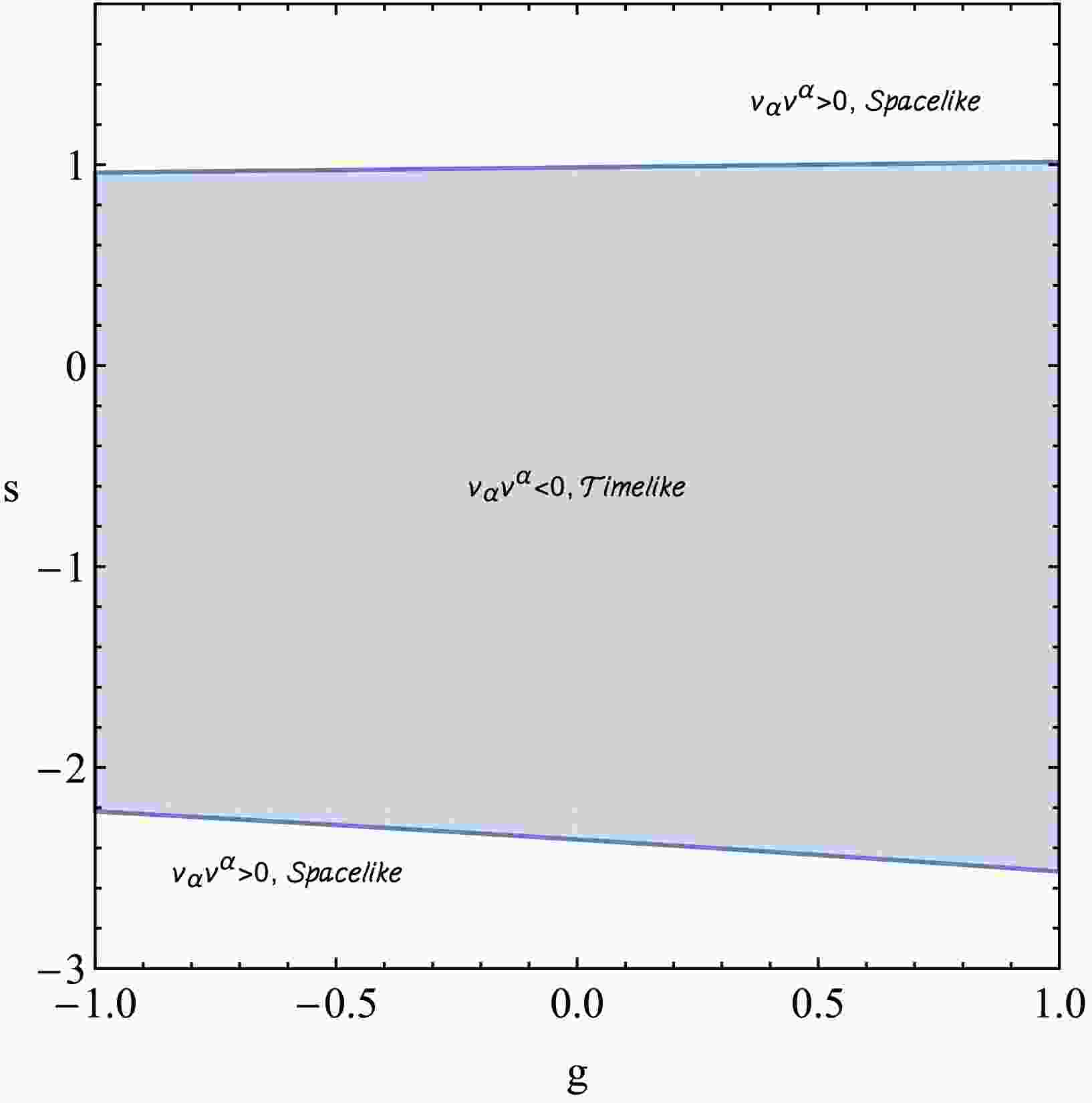
$ r>2 $ and$ Q_m^2<2 $ ,$ h(r)>0 $ , and therefore$ \Delta(r)>1 $ . Thus,$ \Delta>0 $ holds everywhere in the nonextremal exterior and imposes no additional boundary. Consequently, the admissible domain shown below is determined solely by the causality condition$ v_\alpha v^\alpha<0 $ .Figure 1 shows that the timelike domain is bounded by two branches,
$ s_-(g) $ and$ s_+(g) $ , corresponding to the null condition$ v_\alpha v^\alpha=0 $ . Its dependence on the monopole coupling is strongly asymmetric with respect to spin orientation. The upper boundary remains close to$ s\simeq1 $ and varies only weakly over the displayed interval of g, whereas the lower boundary shifts to more negative values of s as g increases. Thus, the monopole interaction modifies the formal causality limit predominantly for the negative-spin branch.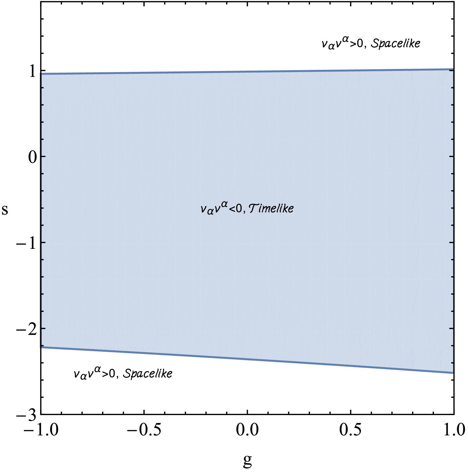
Figure 1. (color online) Causality-preserving domain in the
$ (g,s) $ plane for the equatorial circular motion of a spinning magnetic monopole in the Einstein-frame GMGHS spacetime. The shaded region satisfies$ v_\alpha v^\alpha<0 $ , and the boundary curves are defined by$ v_\alpha v^\alpha=0 $ . Outside the shaded region, the kinematic tangent vector is spacelike. All other orbital and black-hole parameters are held fixed throughout the scan.This asymmetry follows from the sign-dependent spin structure of the Tulczyjew momentum–velocity relation. The monopole contribution enters the conserved momentum through
$ gQ_m $ , while spin enters both through the spin–curvature terms and through the axial constant$ {\cal{J}}={\cal{L}}+s $ . Reversing the sign of s therefore changes how the temporal and azimuthal momentum components combine in the kinematic tangent. Consequently, the two null boundaries need not occur at equal values of$ |s| $ , nor need they respond equally to variations in g.For
$ Q_m>0 $ , increasing g moves the system toward the repulsive monopole sector. In the configuration shown in Fig. 1, this produces only a small displacement of the positive-spin boundary but allows the negative-spin branch to remain timelike up to a larger$ |s| $ . The effect is therefore not a uniform widening of the causal band; rather, it redistributes the admissible spin interval between the two orientations.The null curves define the formal causality boundary of the MPD system, not the domain of quantitative validity of the pole–dipole approximation. The latter additionally requires the characteristic spin length to remain small compared with the black-hole scale,
$ |s|/M\ll1 $ . We therefore retain only the large-$ |s| $ portions of Fig. 1 to show the structure of the causality boundary, while interpreting the orbital and collision calculations in the small-spin regime. -
The radial motion is governed by the positive-energy branch,
$ V_{{\rm{eff}}}=V_+ $ , derived in Sec. II B. A circular orbit at$ r=r_c $ satisfies$ {\cal{E}}=V_{{\rm{eff}}}(r_c), \qquad \left. \frac{\partial V_{{\rm{eff}}}}{\partial r} \right|_{r_c}=0. $
(67) A local minimum of
$ V_{{\rm{eff}}} $ corresponds to stable circular motion, whereas a local maximum corresponds to unstable circular motion. The coalescence of these extrema determines the marginally stable orbit.The upper panels of Fig. 2 show that the effective-potential structure becomes strongly orientation-dependent as the spin approaches the limits of the timelike domain. For positive s, the inner maximum increases, whereas the outer minimum becomes shallower and is no longer resolved within the displayed radial interval for the largest spin values. Thus, the strong-field barrier persists, but the potential well supporting the usual stable circular branch is suppressed.
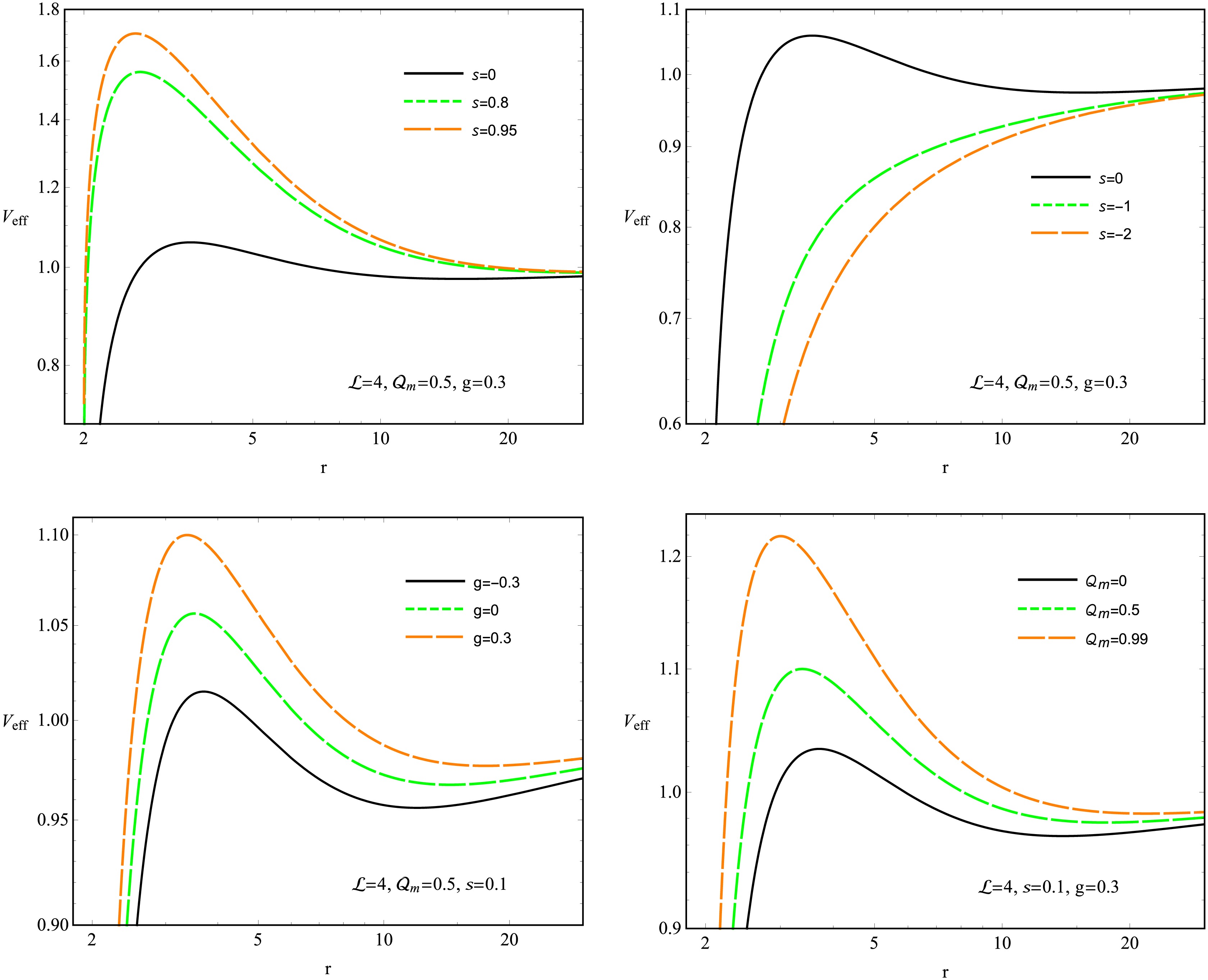
Figure 2. (color online) Radial profiles of the effective potential
$ V_{{\rm{eff}}} $ for equatorial motion of a spinning magnetic monopole in the Einstein-frame GMGHS spacetime. The top-left panel shows$ s=0,\,0.8,\,0.95 $ for fixed$ {\cal{L}}=4 $ ,$ Q_m=0.5 $ , and$ g=0.3 $ . The top-right panel shows$ s=0,\,-1,\,-2 $ , with the remaining parameters held fixed at the same values. The bottom-left panel shows$ g=-0.3,\,0,\,0.3 $ for fixed$ {\cal{L}}=4 $ ,$ Q_m=0.5 $ , and$ s=0.1 $ . The bottom-right panel shows$ Q_m=0,\,0.5,\,0.99 $ for fixed$ {\cal{L}}=4 $ ,$ s=0.1 $ , and$ g=0.3 $ . The upper panels illustrate the approach to the formal causal boundaries; the quantitative pole–dipole interpretation is restricted to the small-spin regime.The negative-spin branch behaves differently. As s becomes more negative, the maximum–minimum pair present for
$ s=0 $ is lost over the displayed radial range, and$ V_{{\rm{eff}}} $ approaches its asymptotic value monotonically from below. The two spin orientations therefore do not approach the causal boundary symmetrically. This behavior is consistent with the signed-spin dependence of the MPD momentum map and with the asymmetric timelike domain found in Fig. 1.These large-spin curves probe the formal boundary of the MPD system rather than the quantitatively controlled pole–dipole regime. In the moderate-spin domain used for the orbital analysis, the maximum–minimum structure remains continuous; however, near the causal boundary, the extrema can become strongly displaced or disappear within the radial interval relevant to bound motion.
The bottom-left panel isolates the monopole coupling for small spin. For
$ Q_m>0 $ , increasing g raises$ V_{{\rm{eff}}} $ , whereas negative g lowers it. The maximum and minimum remain present throughout the displayed range. The leading contribution$ gQ_m/r $ identifies$ gQ_m>0 $ and$ gQ_m<0 $ with the repulsive and attractive monopole sectors, respectively, and explains why the coupling remains appreciable over a broader radial interval than the spin correction.The bottom-right panel shows the dependence on the black-hole magnetic charge. In the Einstein frame,
$ Q_m $ does not enter the redshift factor$ g_{tt}=-f(r) $ ; instead, it modifies the angular geometry through$ g_{\varphi\varphi}=r^2h(r) $ and simultaneously changes the monopole interaction through$ gQ_m $ . The same structure is already evident in the spinless limit.$ V_{{\rm{eff}}}^{(s=0)} = \frac{gQ_m}{r} + \sqrt{ f(r) \left[ 1+ \frac{{\cal{L}}^2}{r^2h(r)} \right] }. $
(68) For
$ g>0 $ , increasing$ Q_m $ strengthens the repulsive monopole term and decreases$ h(r) $ , thereby enhancing the angular contribution. Consequently, the inner barrier grows, while the maximum–minimum structure remains intact over the displayed charge interval.Figure 2 therefore distinguishes two regimes. In the moderate-spin domain, variations in g and
$ Q_m $ continuously deform the extrema without changing the qualitative circular-orbit structure. By contrast, as the formal spin boundary is approached, spin–curvature effects can suppress or remove the potential well itself. The main orbital conclusions presented below are therefore drawn from the small-spin regime, while the upper panels characterize the approach to the boundary of the timelike MPD domain. -
The ISCO is determined by the marginal-stability conditions.
$ {\cal{E}}=V_{{\rm{eff}}}(r_{{\rm{ISCO}}}), \qquad \left. \frac{\partial V_{{\rm{eff}}}}{\partial r} \right|_{r_{{\rm{ISCO}}}}=0, \qquad \left. \frac{\partial^2V_{{\rm{eff}}}}{\partial r^2} \right|_{r_{{\rm{ISCO}}}}=0. $
(69) For prescribed values of
$ (s,g,Q_m) $ , these equations determine$ \left( r_{{\rm{ISCO}}}, {\cal{L}}_{{\rm{ISCO}}}, {\cal{E}}_{{\rm{ISCO}}} \right). $
(70) We retain only timelike solutions. Since
$ \Delta(r)>1 $ throughout the nonextremal exterior, the momentum-map regularity condition imposes no additional restrictions.The top row of Fig. 3 shows that increasing s moves the ISCO inward and reduces
$ {\cal{L}}_{{\rm{ISCO}}} $ for all displayed values of g. This dependence remains smooth as the causal boundary is approached, although$ r_{{\rm{ISCO}}} $ becomes appreciably nonlinear. The change in$ {\cal{L}}_{{\rm{ISCO}}} $ is much stronger than that in$ {\cal{E}}_{{\rm{ISCO}}} $ , indicating that spin primarily redistributes the angular support required for marginal stability.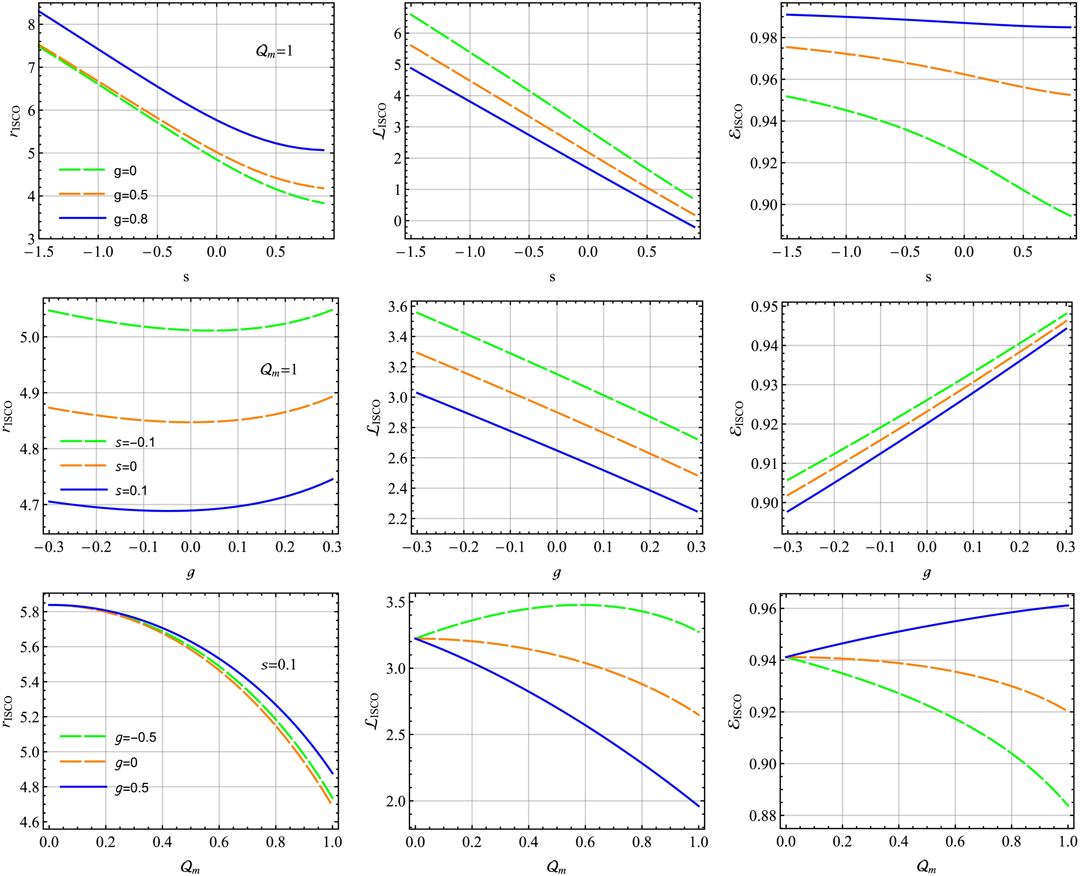
Figure 3. (color online) ISCO radius, orbital angular momentum, and energy for the equatorial motion of a spinning magnetic monopole in the Einstein-frame GMGHS spacetime. Top row: dependence on s for
$ Q_m=1 $ and$ g=0,\,0.5,\,0.8 $ . Middle row: dependence on g for$ Q_m=1 $ and$ s=-0.1,\,0,\,0.1 $ . Bottom row: dependence on$ Q_m $ for$ s=0.1 $ and$ g=-0.5,\,0,\,0.5 $ .The energy is most sensitive to spin in the absence of monopole coupling. As positive g increases,
$ {\cal{E}}_{{\rm{ISCO}}} $ becomes progressively less dependent on s, while$ r_{{\rm{ISCO}}} $ is displaced outward and$ {\cal{L}}_{{\rm{ISCO}}} $ decreases. The repulsive monopole interaction therefore weakens the binding while supplying part of the radial support otherwise provided by orbital motion.The behavior near the causal boundary differs from that of the fixed-
$ {\cal{L}} $ effective potential in Fig. 2. In that case, the potential well may be strongly suppressed at large$ |s| $ , whereas the ISCO remains a smooth marginal solution because$ r_{{\rm{ISCO}}} $ ,$ {\cal{E}}_{{\rm{ISCO}}} $ , and$ {\cal{L}}_{{\rm{ISCO}}} $ are determined simultaneously. Thus, the disappearance of a minimum at fixed$ {\cal{L}} $ does not imply termination of the marginally stable branch.The middle row shows the dependence on the monopole coupling at
$ Q_m=1 $ . The orbital angular momentum decreases and the energy increases monotonically with g, while$ r_{{\rm{ISCO}}} $ develops a shallow minimum. Consequently, the radial position is determined by the full marginal-stability balance rather than by the monopole force alone. Positive spin shifts the corresponding solutions toward smaller radii and lower$ {\cal{L}}_{{\rm{ISCO}}} $ .The bottom row shows the effect of the black-hole magnetic charge. All branches coincide at
$ Q_m=0 $ , where the monopole interaction vanishes and the geometry reduces to Schwarzschild. Increasing$ Q_m $ decreases$ r_{{\rm{ISCO}}} $ even for$ g=0 $ , showing that the Einstein-frame angular deformation already produces an inward displacement.The monopole interaction modifies this geometric tendency according to the sign of g. For
$ g>0 $ , the repulsive interaction partly opposes the inward displacement and raises$ {\cal{E}}_{{\rm{ISCO}}} $ , whereas for$ g<0 $ , the attractive interaction strengthens the binding and permits marginally stable motion at smaller radii. The corresponding behavior of$ {\cal{L}}_{{\rm{ISCO}}} $ reflects the same competition: it decreases rapidly for positive g, while in the attractive sector a broad maximum appears at intermediate$ Q_m $ .The ISCO is therefore governed by the combined redistribution of orbital support produced by spin–curvature coupling, monopole interaction, and the charge-dependent angular geometry. The smooth continuation toward the causal boundary characterizes the formal MPD solutions; however, quantitative interpretation remains restricted to the small-spin regime required by the pole–dipole approximation.
-
We consider collisions between two spinning magnetic monopoles of equal rest mass,
$ m_1=m_2=m, $
(71) with, in general, different specific energies
$ {\cal{E}}_i $ , conserved axial angular momenta$ {\cal{J}}_i $ , and monopole couplings$ g_i\equiv\frac{q_{m,i}}{m}, $
(72) and signed specific spin parameters
$ s_i $ . Each particle obeys the pole–dipole MPD equations in the same fixed Einstein-frame GMGHS background. We neglect mutual gravitational and electromagnetic interactions between the particles.The covariant components of the momentum
$ u^{(i)}_\mu\equiv\frac{p^{(i)}_\mu}{m} $
(73) are given by the relations derived in Sec. II B. The monopole interaction enters through the products
$ g_iQ_m $ , whereas the spin dependence is captured by the spin–curvature terms and the Tulczyjew momentum map.At the collision event,
$ P^\mu=p^\mu_{(1)}+p^\mu_{(2)}, $
(74) and the center-of-mass energy is
$ E_{{\rm{cm}}}^2=-P_\mu P^\mu. $
(75) For equal rest masses, it is convenient to introduce
$ {\cal{E}}_{{\rm{cm}}}^2 \equiv \frac{E_{{\rm{cm}}}^2}{2m^2} = 1-g^{\mu\nu} u^{(1)}_\mu u^{(2)}_\nu. $
(76) For equatorial motion in the Einstein-frame metric,
$ {\cal{E}}_{{\rm{cm}}}^2 = 1 -g^{tt}u^{(1)}_t u^{(2)}_t -g^{rr}u^{(1)}_r u^{(2)}_r -g^{\varphi\varphi} u^{(1)}_\varphi u^{(2)}_\varphi. $
(77) Thus, the collision energy is determined by the mismatch among the temporal, radial, and azimuthal momentum components at the common collision radius. Particles with nearly parallel local momenta produce a smaller
$ {\cal{E}}_{{\rm{cm}}} $ , whereas spin or monopole interactions that separate their local momentum states increase the relative boost and, consequently, the collision energy.Both trajectories must be physically admissible at the collision point. Accordingly, each particle must satisfy
$ v^{(i)}_\alpha v_{(i)}^\alpha<0, $
(78) together with the radial accessibility condition
$ \left(u^r_{(i)}\right)^2\geq0. $
(79) No separate condition on
$ \Delta_i $ is required because$ \Delta_i(r)>1 $ throughout the nonextremal exterior. These conditions ensure that both particles can reach the collision radius along timelike MPD trajectories. -
For fixed values of
$ {\cal{E}} $ , s, g, and$ Q_m $ , access to the strong-field region is determined by the contravariant radial momentum derived in Sec. II B. At the capture threshold, the outer turning point becomes a double root of$ (u^r)^2 $ ,$ { \left. \left(u^r\right)^2 \right|_{r=r_{{\rm{cr}}}} =0, \qquad \left. \frac{d\left(u^r\right)^2}{dr} \right|_{r=r_{{\rm{cr}}}} =0. } $
(80) These conditions determine the critical radius
$ r_{{\rm{cr}}} $ and the critical orbital angular momentum$ {\cal{L}}_{{\rm{cr}}} $ . For the positive-angular-momentum branch considered here,$ {\cal{L}}>{\cal{L}}_{{\rm{cr}}} $ corresponds to reflection at the outer barrier, whereas$ {\cal{L}}\leq{\cal{L}}_{{\rm{cr}}} $ allows the particle to enter the strong-field region.Figure 4 shows that the capture threshold depends on the same three factors that govern circular motion: spin–curvature coupling, the intrinsic monopole interaction, and the charge-dependent deformation of the Einstein-frame geometry. The quantity
$ {\cal{L}}_{{\rm{cr}}} $ is the largest orbital angular momentum for which inward motion remains possible. Its variation therefore measures how the spin and monopole sectors reshape the effective barrier.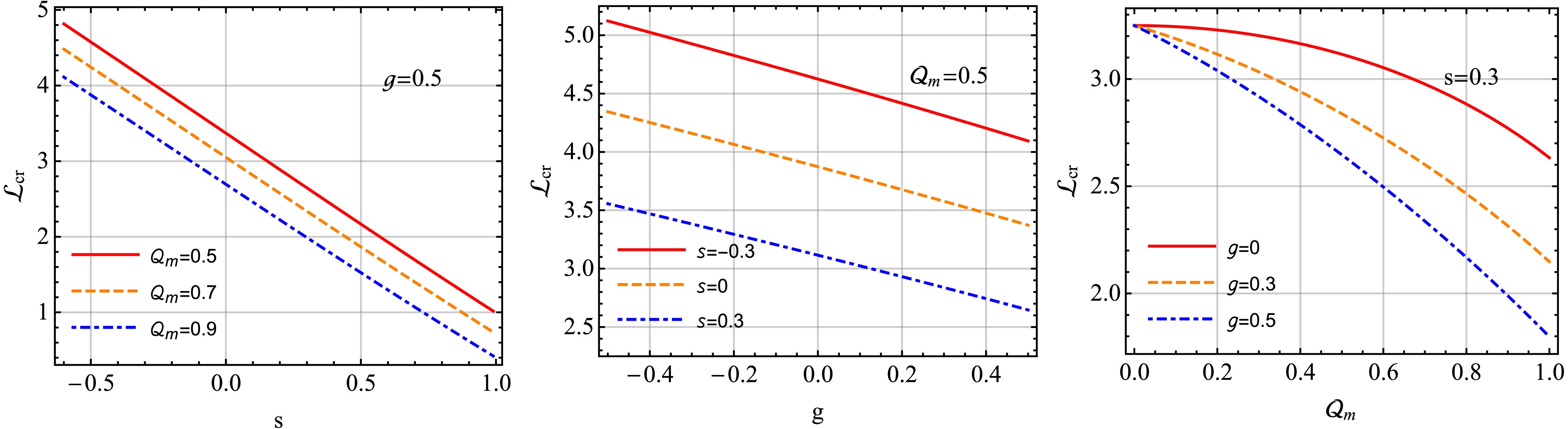
Figure 4. (color online) Critical orbital angular momentum
$ {\cal{L}}_{{\rm{cr}}} $ for the equatorial motion of a spinning magnetic monopole in the Einstein-frame GMGHS spacetime. Left panel: dependence on s for$ Q_m=0.5,\,0.7,\,0.9 $ with fixed$ g=0.5 $ . Middle panel: dependence on g for$ s=-0.3,\,0,\,0.3 $ with fixed$ Q_m=0.5 $ . Right panel: dependence on$ Q_m $ for$ g=0,\,0.3,\,0.5 $ with fixed$ s=0.3 $ . The specific energy is fixed in all three panels.The left panel shows the dependence on the signed spin for three values of
$ Q_m $ at fixed$ g=0.5 $ .$ {\cal{L}}_{{\rm{cr}}} $ decreases nearly linearly with increasing s over the displayed interval. The critical branch remains smooth and regular toward the positive-spin end of this interval, with no indication of a singularity or termination before the formal causal boundary. With the adopted orientation convention, positive spin strengthens the effective support opposing inward motion; thus, the outer barrier can prevent penetration at a smaller orbital angular momentum. Negative spin acts in the opposite sense, allowing the particle to retain a larger$ {\cal{L}} $ while still reaching the inner region. The shift of the curves toward smaller$ {\cal{L}}_{{\rm{cr}}} $ as$ Q_m $ increases reflects the combined effect of geometric deformation and the repulsive monopole contribution for$ gQ_m>0 $ .The middle panel isolates the dependence on the monopole coupling at fixed
$ Q_m=0.5 $ . The critical angular momentum decreases monotonically with g for all three spin orientations. This behavior follows directly from the sign of the monopole force. Positive g produces an outward contribution that assists reflection and reduces the orbital angular momentum required to reach the capture threshold, whereas negative g favors inward motion and therefore raises$ {\cal{L}}_{{\rm{cr}}} $ . The ordering of the three branches remains unchanged throughout: positive spin gives the smallest threshold, negative spin gives the largest, and the spinless case lies between them.The right panel shows the dependence on the black-hole magnetic charge. All three branches meet at
$ Q_m=0 $ , where the spacetime reduces to Schwarzschild and the monopole interaction vanishes independently of g. This common limit provides a direct consistency check. For$ g=0 $ ,$ {\cal{L}}_{{\rm{cr}}} $ decreases with$ Q_m $ solely because of the Einstein-frame deformation of the angular sector. For positive g, the repulsive monopole term proportional to$ gQ_m $ has the same effect, so the decrease becomes more pronounced as the coupling grows.The behavior of
$ {\cal{L}}_{{\rm{cr}}} $ therefore admits a simple interpretation. Spin changes the orbital support needed to balance the inward motion near the outer barrier. The sign of$ gQ_m $ determines whether the intrinsic monopole interaction assists or opposes penetration. The black-hole charge$ Q_m $ enters in both ways: it sets the strength of the monopole sector and simultaneously deforms the Einstein-frame geometry. The interplay of these effects fixes the critical angular momentum. -
The radial dependence of the collision energy is determined by the invariant relative momentum of the two particles. For the noncritical configurations considered below,
$ {\cal{E}}_{{\rm{cm}}}^{2} $ increases toward the strong-field region and remains finite throughout the common admissible radial domain. Spin and monopole interactions modify this profile by altering the particles' temporal, radial, and azimuthal momentum components in distinct ways.The left panel of Fig. 5 shows the effect of the second particle's monopole coupling. For
$ g_1>0 $ , the collision energy is largest when$ g_2<0 $ and smallest when$ g_2>0 $ . Monopole couplings with the same sign shift the two local momentum states in the same direction, whereas couplings with opposite signs drive them apart. The latter configuration therefore yields a larger invariant relative momentum and, consequently, a larger$ {\cal{E}}_{{\rm{cm}}}^{2} $ . The curves separate more clearly away from the horizon, although the common strong-field growth remains dominant.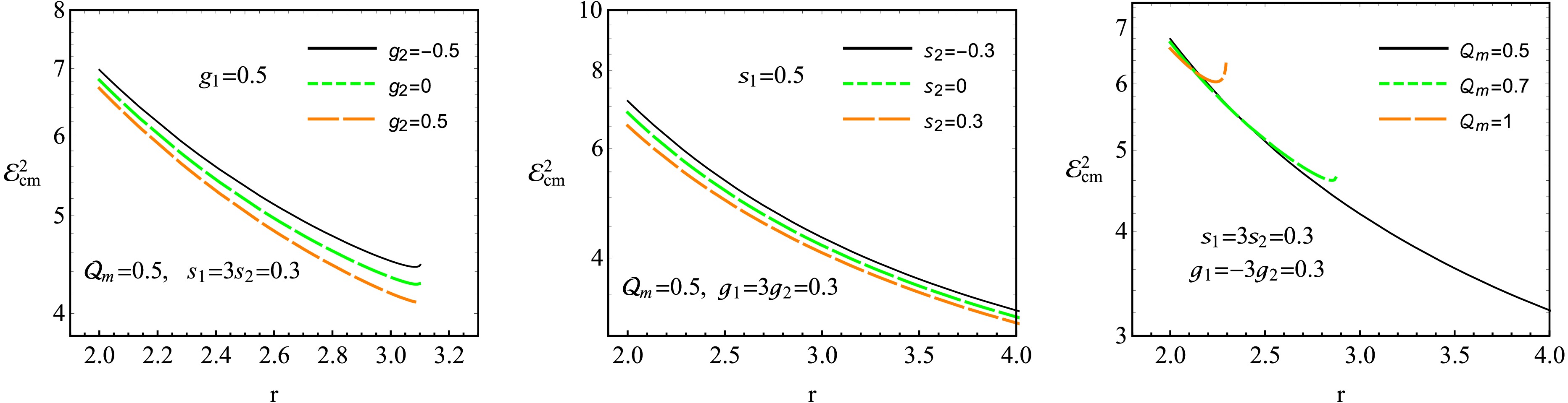
Figure 5. (color online) Radial profiles of the squared center-of-mass energy,
$ {\cal{E}}_{{\rm{cm}}}^{2} $ , for equatorial collisions of two spinning magnetic monopoles in the Einstein-frame GMGHS spacetime. The left panel shows$ g_2=-0.5,\,0,\,0.5 $ with fixed$ Q_m=0.5 $ ,$ g_1=0.5 $ ,$ s_1=0.3 $ , and$ s_2=0.1 $ . The middle panel shows$ s_2=-0.3,\,0,\,0.3 $ with fixed$ Q_m=0.5 $ ,$ g_1=0.3 $ ,$ g_2=0.1 $ , and$ s_1=0.5 $ . The right panel shows$ Q_m=0.5,\,0.7,\,1 $ with fixed$ g_1=0.3 $ ,$ g_2=-0.1 $ ,$ s_1=0.3 $ , and$ s_2=0.1 $ . The remaining constants of motion are held fixed in the corresponding panels.The middle panel shows the corresponding dependence on the signed spin of the second particle. With
$ s_1>0 $ , negative$ s_2 $ yields the largest collision energy, whereas positive$ s_2 $ yields the smallest. Reversing the spin orientation changes the spin–curvature contribution and the second particle's Tulczyjew momentum map relative to the first. Opposite spin orientations therefore produce a larger mismatch between the local momenta. In contrast to the monopole-coupling dependence, the spin-induced separation is strongest at small radii, where curvature effects are most pronounced.The right panel shows the role of the black-hole magnetic charge. In the Einstein frame,
$ Q_m $ does not modify the lapse function$ g_{tt}=-f(r) $ ; instead, its influence enters through the angular geometry$ g_{\varphi\varphi}=r^2h(r) $ , the curvature, and the intrinsic monopole combinations$ g_iQ_m $ . Because$ g_1 $ and$ g_2 $ have opposite signs, increasing$ Q_m $ enhances the difference between their monopole responses. The overlapping parts of the profiles therefore remain close near the horizon but separate as the charge-dependent dynamics becomes more important.A further effect of
$ Q_m $ is to reduce the radial interval accessible to both particles. The$ Q_m=0.5 $ profile extends to larger radii, whereas the$ Q_m=0.7 $ and$ Q_m=1 $ branches terminate progressively closer to the black hole. These endpoints are determined by the radial accessibility condition$ (u^r_i)^2\geq0 $ together with the timelikeness of the two trajectories. Near such an endpoint, one radial momentum approaches zero; the resulting loss of radial co-motion can produce the shallow minimum and subsequent increase visible on the largest-$ Q_m $ branch before the admissible collision domain ends.Figure 5 thus shows that the collision energy depends on the relative response of the two particles rather than on the magnitude of an individual coupling. Opposite monopole signs and opposite spin orientations increase the local momentum mismatch, whereas similar responses reduce it. The black-hole magnetic charge additionally controls the angular geometry and the range of radii at which both particles can participate in the collision.
-
Finally, we consider collisions in which both particles occupy the same marginally stable circular orbit. The first particle determines the reference ISCO radius. For prescribed
$ s_1 $ ,$ g_1 $ , and$ Q_m $ ,$ {\cal{E}}_1 = V_{{\rm{eff}}}^{(1)}(r_{{\rm{ISCO}}}), \quad \left. \frac{\partial V_{{\rm{eff}}}^{(1)}}{\partial r} \right|_{r_{{\rm{ISCO}}}} =0, \quad \left. \frac{\partial^2V_{{\rm{eff}}}^{(1)}}{\partial r^2} \right|_{r_{{\rm{ISCO}}}} =0, $
(81) These conditions determine
$ r_{{\rm{ISCO}}} $ ,$ {\cal{E}}_1 $ , and$ {\cal{L}}_1 $ . The second particle must be marginally stable at the same radius and therefore satisfies the following conditions:$ {\cal{E}}_2 = V_{{\rm{eff}}}^{(2)}(r_{{\rm{ISCO}}}), \quad \left. \frac{\partial V_{{\rm{eff}}}^{(2)}}{\partial r} \right|_{r_{{\rm{ISCO}}}} =0, \quad \left. \frac{\partial^2V_{{\rm{eff}}}^{(2)}}{\partial r^2} \right|_{r_{{\rm{ISCO}}}} =0. $
(82) Thus, the two particles have the same ISCO radius, whereas their conserved quantities and non-geodesic couplings may differ. In the left panel of Fig. 6,
$ s_2 $ is varied, and the corresponding$ g_2 $ ,$ {\cal{E}}_2 $ , and$ {\cal{L}}_2 $ are obtained from Eq. (82). In the right panel,$ g_2 $ is varied, and$ s_2 $ ,$ {\cal{E}}_2 $ , and$ {\cal{L}}_2 $ are determined in the same manner.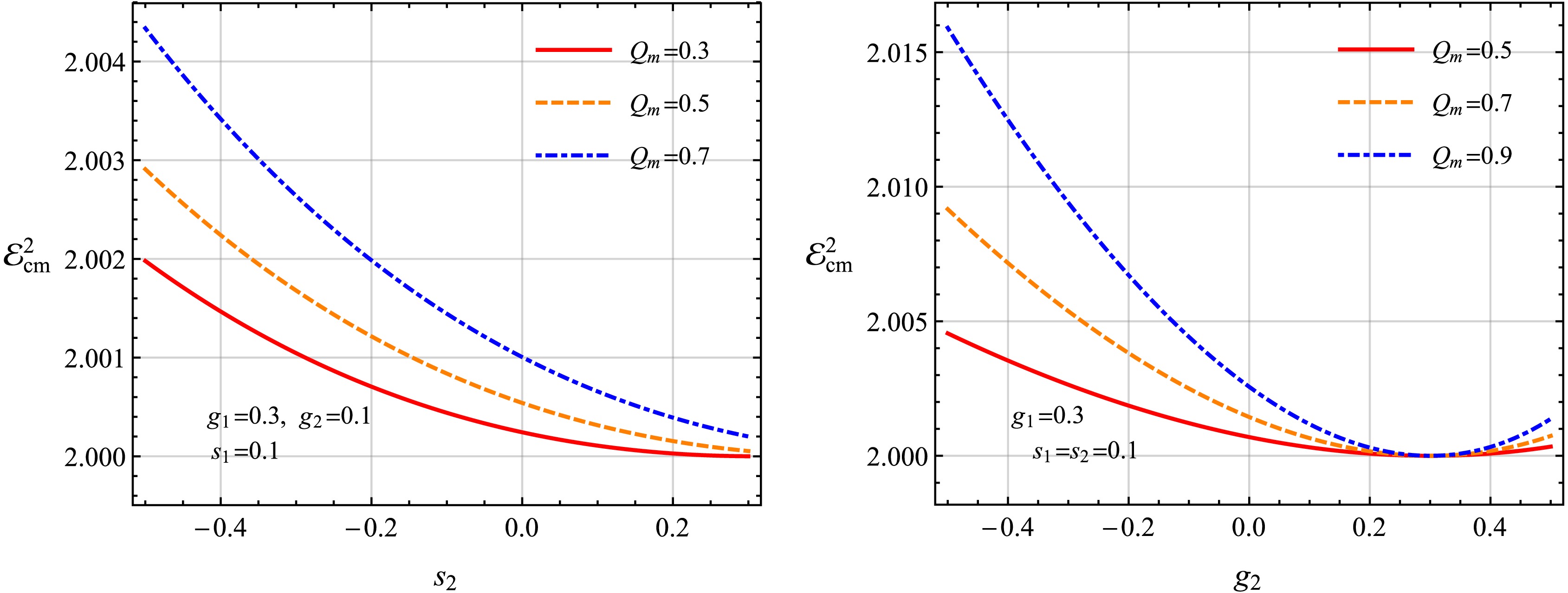
Figure 6. (color online) Squared center-of-mass energy
$ {\cal{E}}_{{\rm{cm}}}^{2} $ for collisions between two spinning magnetic monopoles at a common ISCO radius. Left panel: dependence on$ s_2 $ for selected values of$ Q_m $ , with$ g_2 $ ,$ {\cal{E}}_2 $ , and$ {\cal{L}}_2 $ determined by the common marginal-stability conditions. Right panel: dependence on$ g_2 $ for selected values of$ Q_m $ , with$ s_2 $ ,$ {\cal{E}}_2 $ , and$ {\cal{L}}_2 $ determined by the same conditions. The parameters of particle 1 are fixed as indicated in the panels.Because both trajectories are circular at the collision point,
$ u^r_{(1)}=u^r_{(2)}=0, $
(83) and the center-of-mass energy reduces to
$ {\cal{E}}_{{\rm{cm}}}^{2} = 1 -g^{tt}u_t^{(1)}u_t^{(2)} -g^{\varphi\varphi}u_\varphi^{(1)}u_\varphi^{(2)}. $
(84) The collision energy therefore quantifies only the mismatch between the temporal and azimuthal momentum components of the two marginally stable motions.
Figure 6 shows that the center-of-mass energy remains finite and close to the comoving value
$ {\cal{E}}_{{\rm{cm}}}^{2}=2 $ . The common ISCO conditions strongly constrain the relative motion: both radial momenta vanish, and the remaining difference is confined to the temporal and azimuthal components. Consequently, the collision energy is much less sensitive to the particle parameters than in collisions involving distinct radial trajectories.In the left panel, changing
$ s_2 $ alters the spin–curvature contribution to the marginal-stability balance. Because particle 1 fixes the radius, this change must be compensated by corresponding adjustments to$ g_2 $ ,$ {\cal{E}}_2 $ , and$ {\cal{L}}_2 $ . Thus, the variation in$ {\cal{E}}_{{\rm{cm}}}^{2} $ measures the residual momentum difference after the monopole and orbital contributions have readjusted to maintain the same ISCO.The right panel shows the complementary balance. Varying
$ g_2 $ changes the intrinsic monopole term by$ g_2Q_m $ , while the common ISCO conditions require simultaneous adjustments to$ s_2 $ ,$ {\cal{E}}_2 $ , and$ {\cal{L}}_2 $ . The resulting collision energy therefore reflects the coupled spin–monopole response rather than either interaction acting independently.The value
$ {\cal{E}}_{{\rm{cm}}}^{2}=2 $ is obtained when the two local four-momenta coincide. In the identical-particle limit,$ {\cal{E}}_2={\cal{E}}_1 $ ,$ {\cal{L}}_2={\cal{L}}_1 $ ,$ s_2=s_1 $ , and$ g_2=g_1 $ , so that$ u_\mu^{(2)}=u_\mu^{(1)} $ . Departures from this value quantify the residual difference between two distinct marginally stable momentum states occupying the same circular orbit.The role of
$ Q_m $ is twofold. It modifies the Einstein-frame angular geometry through$ g_{\varphi\varphi}=r^2h(r) $ and the curvature entering the spin interaction, while also setting the strength of the monopole terms$ g_iQ_m $ . The compensation required to preserve a common ISCO therefore changes with$ Q_m $ , as does the relative momentum of the colliding particles. Because$ g_{tt}=-f(r) $ is independent of$ Q_m $ , this dependence is not associated with a charge-dependent redshift.Collisions at a common ISCO are therefore governed by a constrained balance between spin–curvature and monopole interactions. The marginal-stability conditions suppress large relative boosts, while the finite deviations of
$ {\cal{E}}_{{\rm{cm}}}^{2} $ from 2 measure the remaining difference between the two admissible ISCO momentum states. -
We investigated the equatorial dynamics and collision energetics of spinning magnetic monopoles in the spacetime of a magnetically charged stringy black hole in the Einstein frame. We described the motion in the pole–dipole approximation using the Mathisson–Papapetrou–Dixon equations with the Tulczyjew–Dixon spin supplementary condition and an intrinsic monopole coupling to the dual electromagnetic field generated by the black-hole magnetic charge
$ Q_m $ . From the conserved quantities and momentum normalization, we derived the radial first integral and constructed the effective potential. We selected physical trajectories by requiring a timelike kinematic tangent,$ v_\mu v^\mu<0 $ , together with radial accessibility. In the nonextremal exterior, the Tulczyjew momentum map remains regular because$ \Delta(r)>1 $ .The causality analysis showed that the admissible spin interval is asymmetric with respect to spin orientation. Increasing the monopole coupling primarily changes the negative-spin boundary, whereas the positive-spin limit varies only weakly over the displayed range. This behavior follows from the simultaneous appearance of the signed spin in the spin–curvature terms and in the total axial angular momentum
$ {\cal{J}}={\cal{L}}+s $ . The large-$ |s| $ portions of the causal domain characterize the formal MPD boundary; therefore, we interpreted the orbital and collision results in the small-spin regime appropriate for the pole–dipole approximation.The effective potential distinguishes the roles of spin, monopole interaction, and stringy geometry. At fixed
$ {\cal{L}} $ , spin predominantly reshapes the strong-field barrier, with the two spin orientations producing markedly different behavior near the causal boundary. The monopole interaction depends on the product$ gQ_m $ : positive$ gQ_m $ contributes outward and weakens binding, whereas negative$ gQ_m $ favors stronger binding. The black-hole magnetic charge acts through both this intrinsic monopole interaction and the Einstein-frame angular geometry$ g_{\varphi\varphi}=r^2h(r) $ and its associated curvature. It does not modify the lapse function$ g_{tt}=-f(r) $ .The ISCO analysis showed that spin mainly redistributes the angular support required for marginal stability. Increasing s moves
$ r_{{\rm{ISCO}}} $ inward and substantially decreases$ {\cal{L}}_{{\rm{ISCO}}} $ over the displayed range, whereas$ {\cal{E}}_{{\rm{ISCO}}} $ varies more weakly. At fixed$ Q_m $ , increasing g lowers$ {\cal{L}}_{{\rm{ISCO}}} $ and raises$ {\cal{E}}_{{\rm{ISCO}}} $ , while$ r_{{\rm{ISCO}}} $ exhibits a shallow nonmonotonic dependence. The dependence on$ Q_m $ reflects the competition between the angular deformation of the Einstein-frame geometry and the monopole interaction. Even for$ g=0 $ , increasing$ Q_m $ moves the ISCO inward, showing that the geometric contribution is already present without monopole coupling. Positive g partly opposes this inward displacement, whereas negative g strengthens the binding and permits marginally stable motion at smaller radii.We also determined the critical orbital angular momentum
$ {\cal{L}}_{{\rm{cr}}} $ that separates capture from reflection. Increasing the signed spin lowers$ {\cal{L}}_{{\rm{cr}}} $ for the orientation considered, whereas negative spin allows capture at larger orbital angular momentum. At fixed$ Q_m>0 $ , increasing g likewise lowers$ {\cal{L}}_{{\rm{cr}}} $ because the repulsive monopole interaction assists reflection. The$ Q_m $ dependence combines the geometric deformation with the monopole contribution and therefore provides a complementary measure of how these two effects control access to the strong-field region.For two-particle collisions, the center-of-mass energy is governed by the invariant mismatch between the local momentum states rather than by the magnitude of any single coupling. The radial profiles show that
$ {\cal{E}}_{{\rm{cm}}}^{2} $ increases toward the strong-field region but remains finite for the noncritical, physically admissible trajectories considered. Opposite monopole responses produce a larger momentum mismatch than like-sign responses, while anti-alignment of the second particle's spin similarly increases the collision energy relative to aligned configurations. Increasing$ Q_m $ modifies both the relative momentum and the radial interval over which the two trajectories remain simultaneously admissible.Collisions at the ISCO remain finite and close to the comoving value
$ {\cal{E}}_{{\rm{cm}}}^{2}=2 $ . The radial momentum vanishes for both particles, so the residual collision energy is determined by the difference between their temporal and azimuthal momentum components. Variations in the second particle's spin or monopole coupling change this mismatch, while increasing$ Q_m $ generally increases the sensitivity of the collision energy to differences between the two particle states. The comoving value is recovered when the local four-momenta coincide.Overall, the results show that spin–curvature coupling, intrinsic monopole interaction, and charge-dependent angular geometry play distinct but coupled roles in determining circular motion, marginal stability, capture, and collision energetics. The magnetically charged stringy black hole therefore provides a useful strong-field setting for studying nongeodesic spinning-particle dynamics in an intrinsic electromagnetic field without introducing an external magnetic field.
Spinning magnetic monopoles in magnetically charged stringy black hole spacetime: spin-curvature & magnetic interaction effects on circular orbits and particle collisions
- Received Date: 2026-08-06
- Available Online: 2027-01-01
Abstract: We investigate the equatorial dynamics and collision energetics of spinning magnetic monopoles around a magnetically charged stringy black hole in the Einstein frame. We describe the motion using the Mathisson–Papapetrou–Dixon equations with the Tulczyjew–Dixon spin supplementary condition and an intrinsic monopole coupling to the black hole's magnetic field. We derive the effective potential and examine the causality domain, circular orbits, ISCO properties, capture threshold, and two-particle collisions. Spin–curvature coupling primarily modifies the angular support required for marginal stability, whereas the monopole interaction is governed by $ gQ_m $, with $ gQ_m>0 $ acting repulsively and $ gQ_m<0 $ promoting stronger binding. The magnetic charge $ Q_m $ also alters the angular geometry and curvature, producing a combined geometric and monopole effect on the ISCO. We determine the critical orbital angular momentum $ {\cal{L}}_{{\rm{cr}}} $ that separates capture from reflection. The center-of-mass energy is determined by the mismatch between the particles' local momenta; opposite monopole couplings and spin orientations generally increase this mismatch. For the physically admissible configurations considered, the collision energy remains finite, including for collisions at the ISCO, where $ {\cal{E}}_{{\rm{cm}}}^{2} $ tends to the comoving value 2.



 DownLoad: