Non-Metricity Corrections Approach to Alleviate H₀ Tension: The Logarithmic and Nonlinear f(Q) Models

The Hubble constant $ H_0 $, which quantifies the present expansion rate of the Universe, has now been measured with remarkable precision, transforming what was once a minor inconsistency into a significant challenge for the standard cosmological model. This discrepancy, commonly referred to as the Hubble tension [1], corresponds to a persistent disagreement-now exceeding the $ 5\sigma $ level-between values of $ H_0 $ inferred from different observational probes [2–4]. The discovery of the late-time accelerated expansion of the Universe through observations of Type Ia supernovae (SNIa) [5, 6] established these objects as powerful distance indicators, forming the basis of the cosmic distance ladder. In particular, late-Universe measurements calibrated via Cepheid variables and SNIa consistently yield a higher value, $ H_0 = 73.04 \pm 1.04\ {\rm{km}}\;{\rm{s}}^{-1}\;{\rm{Mpc}}^{-1} $ [7], further supported by recent analyses incorporating James Webb Space Telescope (JWST) observations [8] and extended distance ladder studies [9]. In contrast, baryon acoustic oscillation (BAO) measurements provide an independent probe of the expansion history by utilizing the sound horizon at the baryon drag epoch, $ r_d \approx 147\;{\rm{Mpc}} $, as a standard ruler [10]. This scale, imprinted in the large-scale distribution of matter and observed in the galaxy two-point correlation function, enables precise constraints on both the comoving angular diameter distance $ D_M(z) $ and the Hubble parameter $ H(z) $ over a wide redshift range. Large spectroscopic surveys such as WiggleZ, SDSS-III BOSS [11–13], and more recently the Dark Energy Spectroscopic Instrument (DESI) have significantly improved the precision of BAO measurements, with the latest DESI Data Release 2 (DR2), covering $ 0.1 \lt z \lt 4.2 $, reporting $ H_0 = 68.51 \pm 0.58\;{\rm{km}}\;{\rm{s}}^{-1}\;{\rm{Mpc}}^{-1} $ [14, 15], in closer agreement with early-Universe estimates. The contrast between the higher values inferred from supernova-based distance ladder measurements and the lower values obtained from BAO lies at the core of the Hubble tension.

More recently, this growing inconsistency has placed increasing pressure on the standard ΛCDM framework [16], motivating a systematic re-examination of its underlying assumptions and possible extensions. A broad class of theoretical approaches has been proposed to address this tension, particularly those that modify the late-time expansion history $ H(z) $ at redshifts $ z \lesssim 2 $ [17–19]. Among these, dynamical dark energy models replace the cosmological constant with a time-dependent component characterized by an evolving equation of state parameter $ w = p/\rho $, thereby introducing additional degrees of freedom that must account for nearly 70 percent of the present energy budget of the Universe [20–24]. While such models raise important questions regarding the physical origin and non-detection of these fields, recent observational developments have renewed interest in these scenarios. In particular, the latest BAO measurements from the DESI collaboration [3, 14, 19, 25, 26], extending earlier results from SDSS surveys, have significantly enhanced the precision of cosmological constraints. Complementary information is provided by Type Ia supernova datasets, including the Pantheon (PN) and Pantheon+SH0ES compilations as well as the Dark Energy Survey five-year sample (DES SN5YR), which offer improved control over systematic uncertainties [27–32]. When combined with local measurements from the SH0ES program, these datasets consistently favor a higher value of $ H_0 $ [33]. Within this observational context, recent Bayesian analyses-especially those incorporating DESI data-have indicated a statistical preference for dynamical dark energy models over the standard ΛCDM scenario [4, 34–36], even after accounting for the presence of additional free parameters. This emerging preference suggests that deviations from a simple cosmological constant ($ w = -1 $) may be favored, potentially providing new insights into the nature of cosmic acceleration and its connection to the Hubble tension [37–41].

An alternative and conceptually distinct approach involves modifying the underlying theory of gravity rather than introducing new energy components. In this context, cosmic acceleration arises from deviations from General Relativity (GR) on large scales, leading to modifications in the expansion history and the inferred cosmological parameters [42–50]. Such theories can, in principle, influence both early and late-time physics either by altering the sound horizon scale or by modifying the late-time dynamics thereby offering additional flexibility in addressing the Hubble tension. Among the various modified gravity frameworks, symmetric teleparallel gravity, or $ f(Q) $ gravity, has recently gained significant attention [51]. In this formulation, gravity is described in terms of the non-metricity scalar Q, and the gravitational action is generalized to an arbitrary function $ f(Q) $, introducing new dynamical degrees of freedom capable of driving cosmic acceleration without invoking a cosmological constant [52–58]. The $ f(Q) $ framework is particularly appealing in the context of the Hubble tension, as it modifies the effective Friedmann equations and can produce deviations in the late-time expansion rate while preserving the well-established predictions of early-Universe cosmology [59–62]. Consequently, these models can effectively mimic dynamical dark energy behavior, including a redshift-dependent equation of state, and offer a viable pathway toward reconciling the discrepancy in $ H_0 $ [63–68]. Recent studies show that EDE motivated by the Hubble tension can increase the inferred $\alpha_s$, strengthening tension with USR-based PBH formation [69]. In another model-independent test, the detection of a Cosmic Graviton Background ($\Delta N_{\rm{eff}},g \simeq0.054$) could rule out realistic inflationary scenarios, offering a potential probe of alternatives such as bouncing and emergent cosmologies [70, 71]. Confronting such models with recent observational datasets including BAO measurements from DESI, supernova compilations such as Pantheon+ and DES SN5YR, and local determinations of the Hubble constant provides a crucial test of whether modifications to gravity can alleviate the tension and yield an improved description of the observed Universe relative to the standard ΛCDM model [1, 3, 18, 72–75].

In this work, we investigate the implications of symmetric teleparallel gravity within the context of the Hubble tension by $ f(Q) $ model with a comprehensive set of late-time observational data. In particular, we consider multiple Type Ia supernova compilations, including the Pantheon, Pantheon+ combined with SH0ES, and the DES SN5YR, which together provide robust constraints on the expansion history over a wide redshift range. These datasets are further complemented by BAO measurements from SDSS and the latest results from the DESI, as well as cosmic chronometer (CC) data that offer direct estimates of the Hubble parameter. The primary objective of this analysis is to examine how modifications arising from symmetric teleparallel gravity, specifically within the framework of $ f(Q) $ theories, influence the late-time expansion dynamics and whether they can alleviate the existing tension in $ H_0 $ measurements. To this end, we consider two representative functional forms of $ f(Q) $: a logarithmic model and a nonlinear saturation model, both of which introduce deviations from the standard ΛCDM behavior through geometric effects.

The structure of the paper is organized as follows. In Section II, we present the theoretical framework of $ f(Q) $ gravity and derive the corresponding cosmological field equations for a homogeneous and isotropic Universe. Section III describes the observational datasets employed in this study and outlines the statistical methodology used for parameter estimation. In Section IV, we introduce the specific functional forms of the proposed models and derive the associated expressions for the Hubble expansion rate. This section also presents the observational constraints obtained within a Bayesian framework using the combined datasets, together with a comparative analysis of Model I and Model II. Finally, in Section V, we summarize the main results and discuss their implications for the Hubble tension, as well as the viability of modified gravity as an alternative to the standard cosmological model.

The action of $ f(Q) $ gravity [51] is given by

where we use natural units in which $ 8\pi G/c^4 = 1 $, and $ S_m $ denotes the matter action. Varying the action with respect to the metric tensor yields the field equations as

where $ f_Q = \partial f/\partial Q $. In addition, variation with respect to the affine connection yields

which governs the dynamics associated with the connection.

The tensor $ P^\alpha_{\mu\nu} $, conjugate to nonmetricity, is defined as

where parentheses denote symmetrization, $ A_{(\mu\nu)} = \frac{1}{2}(A_{\mu\nu} + A_{\nu\mu}) $. The two independent traces of the nonmetricity tensor are defined as

The nonmetricity scalar Q can then be written as

To investigate the cosmological implications, we consider a spatially flat, homogeneous, and isotropic Friedmann-Lemaître-Robertson-Walker (FLRW) spacetime described by

where $ a(t) $ is the scale factor. In the coincident gauge, the connection coefficients vanish, and the metric is the only dynamical variable. Choosing a different gauge would introduce nontrivial contributions from the connection [51, 71]. For the metric in Eq. (7), the nonmetricity scalar reduces to

where $ H = \dot{a}/a $ denotes the Hubble parameter.

The matter content of the Universe is modeled as a perfect fluid with energy-momentum tensor

where ρ and p denote the energy density and pressure, respectively, and $ u_\mu $ is the four-velocity of the fluid. Substituting the FLRW metric into the field equations yields the modified Friedmann equations

These equations determine the cosmological dynamics in $ f(Q) $ gravity.

With the decomposition $ f(Q) = Q + \Phi(Q) $, the preceding equations can be rewritten as

Constructing a viable cosmological model requires specifying a functional form for $ \Phi(Q) $.

To constrain the model parameters, we perform a Bayesian analysis using a Markov chain Monte Carlo (MCMC) approach implemented with the publicly available $\mathrm{emcee}$ package [76], which uses an affine-invariant ensemble sampler. This algorithm is well suited to efficiently exploring correlated, high-dimensional parameter spaces. The posterior probability distribution is given by $ {\cal{P}}(\Theta|D) \propto {\cal{L}}(D|\Theta)\,\Pi(\Theta) $, where $ {\cal{L}} $ denotes the likelihood function and $ \Pi(\Theta) $ represents the prior on the parameter vector Θ. Assuming Gaussian-distributed observational uncertainties, the total likelihood is expressed in terms of the combined chi-square as

We evolve multiple chains (walkers) in parallel to ensure appropriate sampling of the posterior distribution. Convergence is assessed using standard diagnostics, including the stabilization of chain means and the integrated autocorrelation time. Only samples from the converged, post-burn-in phase are used to derive parameter constraints.

Cosmic Chronometers (CC): We use a compilation of 31 measurements of the Hubble parameter obtained using the CC technique [77, 78]. This method provides direct estimates of $ H(z) $ by measuring the differential age evolution of passively evolving galaxies and exploiting the relation $ H(z) = -\frac{1}{1+z}\frac{dz}{dt} $. Because it relies on relative age differences, $ \Delta z/\Delta t $, it is less sensitive to systematic uncertainties than methods based on absolute age determinations [37, 79, 80]. Galaxy age estimates are based on well-calibrated stellar population synthesis models [81–84], and the method remains largely independent of any assumed cosmological model or distance ladder calibration. The corresponding chi-square function is given by

where $ H(z_i,\Theta) $ and $ H_{\text{obs}}(z_i) $ denote the theoretical and observed values, respectively, and $ \sigma_{CC}(z_i) $ denotes the measurement uncertainty.

Type Ia Supernovae: Another key dataset employed in our MCMC analysis consists of Type Ia supernova (SNe Ia) observations [5, 6]. These events, which typically originate from thermonuclear explosions in binary systems, are particularly important in cosmology because of their nearly uniform intrinsic luminosity. This property allows them to be used as standardizable candles for measuring distances to high-redshift galaxies, thereby constraining the expansion history of the Universe.

The primary observable in supernova cosmology is the distance modulus, defined as the difference between the apparent magnitude $m$ and the absolute magnitude $M$ [85], given by

where the luminosity distance is given by

Here, $c$ denotes the speed of light, and $H(z,\Theta)$ is the model-dependent Hubble parameter.

In this work, we use two major SNe Ia compilations: the Pantheon dataset and its extended version, Pantheon+ combined with SH0ES [7, 28, 29, 33]. The Pantheon sample comprises 1048 spectroscopically confirmed supernovae spanning the redshift range $0.01 \lt z \lesssim 2.3$, providing a robust baseline for cosmological analysis [27, 86]. The Pantheon+SH0ES compilation extends this dataset to 1701 light-curve measurements from 1550 confirmed SNe Ia [10, 87–89], incorporating Cepheid-calibrated host-galaxy distances from the SH0ES program. This calibration plays a crucial role in breaking the degeneracy between the absolute magnitude $M$ and the Hubble constant $H_0$, thereby enabling tighter constraints on cosmological parameters.

For both the Pantheon and Pantheon+SH0ES datasets, the absolute magnitude $M$ is treated as a nuisance parameter and marginalized over during the MCMC analysis. The theoretical predictions for the distance modulus are compared with observations, and parameter estimation is performed by minimizing the corresponding chi-square function.

where $\Delta \mu = \mu(z_i,\Theta) - \mu_{\text{obs}}(z_i)$, and $C$ denotes the covariance matrix, including both statistical and systematic uncertainties.

In addition to these datasets, we also consider the Dark Energy Survey five-year supernova sample (DES-SN5YR), which comprises 1829 SNe Ia and provides an independent, homogeneous dataset with improved control of observational systematics [30–32]. We use the publicly released DES-SN5YR distance-modulus data together with the corresponding full statistical and systematic covariance matrix. The published distance moduli are constructed using the reference normalization of $ H_0 $ stated in Ref. [90]. This reference value is part of the normalization adopted for the released distance-modulus data and is not imposed as a fixed value or external prior on $ H_0 $ in our analysis.

Since the unanchored DES-SN5YR Hubble diagram does not independently determine the absolute supernova luminosity, the absolute magnitude and $ H_0 $ remain degenerate [32]. Therefore, rather than fixing the absolute magnitude M, we account for the corresponding additive calibration uncertainty by introducing a nuisance offset $ {\cal{M}} $ and analytically marginalizing over it. In particular, defining $ \Delta{\boldsymbol{\mu}}={\boldsymbol{\mu}}_{{\rm{obs}}}-{\boldsymbol{\mu}}_{{\rm{th}}} $, we use

where $ {\bf{C}}_{{\rm{DES}}} $ is the full DES-SN5YR covariance matrix. Assuming a flat prior on $ {\cal{M}} $, this nuisance parameter can be marginalized analytically, yielding

where

Thus, the DES-SN5YR data constrain the relative distance–redshift relation, with the absolute SN calibration marginalized over, thereby avoiding the introduction of an artificial absolute calibration for $ H_0 $. The resulting DES contribution is then combined with the other observational datasets in the total likelihood. For the Pantheon and Pantheon+SH0ES datasets, the absolute magnitude M is explicitly included as a nuisance parameter in the fitting procedure, and the corresponding fitted value is reported in the tables. For DES-SN5YR, we do not report a separate value of M because the absolute SN calibration is marginalized over in the likelihood rather than independently determined from the unanchored DES Hubble diagram.

Baryon Acoustic Oscillations (BAO): In this analysis, we use a combined BAO dataset from several large-scale structure surveys. These comprise the 6dF Galaxy Survey at an effective redshift $ z_{\text{eff}}=0.106 $ [91], the SDSS Main Galaxy Sample at $ z_{\text{eff}}=0.15 $ [92], the BOSS DR11 Lyman-α forest measurement at $ z_{\text{eff}}=2.4 $, the SDSS-IV eBOSS DR14 quasar observations at $ z_{\text{eff}}=\{0.98, 1.23, 1.52,1.94\} $ [93], and the consensus BAO results from SDSS-III BOSS DR12 at $ z_{\text{eff}}=\{0.38,0.51,0.61\} $ [12]. The full covariance matrices associated with these measurements are included in the likelihood analysis to ensure a consistent statistical treatment.

The BAO observables are expressed in terms of the Hubble distance $ D_H(z) $, the comoving angular diameter distance $ D_M(z) $, and the volume-averaged distance $ D_V(z) $, which are defined as

where the angular diameter distance is related to the luminosity distance by $ D_A(z) = (1+z)^{-2}D_L(z) $. These quantities are combined into observable vectors $ F(z_i,\Theta) $, typically normalized by the sound horizon scale at the baryon drag epoch.

An important aspect of BAO analyses is the inherent degeneracy between the sound horizon $ r_d $ and the Hubble constant $ H_0 $. This degeneracy arises because BAO measurements primarily constrain the combination $ c/(H_0 r_d) $, making it difficult to determine these parameters independently from BAO data alone. Breaking this degeneracy requires additional cosmological information or external priors on $ r_d $, often obtained from cosmic microwave background (CMB) measurements or Big Bang nucleosynthesis (BBN) considerations.

In this work, the comoving sound horizon at the drag epoch ($z_d \approx 1059.94$) is evaluated as [94]

where we adopt $ \Omega_{b,0} = 0.02242 $, $ \Omega_{\gamma,0} = 2.469 \times 10 ^{-5} $ [94], $ T_0 = 2.7255\,\text{K} $ [95], and the fiducial value $ r_{s,\text{fid}}(z_d) = 147.05\,\text{Mpc} $. The sound horizon represents the maximum comoving distance that acoustic waves can propagate through the tightly coupled photon–baryon plasma before recombination and therefore provides a standard ruler for BAO measurements. BAO observations thus constrain the expansion history through combinations of the Hubble parameter and the comoving angular-diameter distance, usually expressed in terms of $ D_H(z)=c/H(z) $ and $ D_M(z) $ relative to the sound horizon.

For a given cosmological model, the theoretical BAO quantities are evaluated from the corresponding expansion history $ H(z) $ and compared with the observed measurements. In particular, depending on the type of BAO observable, the relevant quantities can be written as

where

and

Thus, the BAO data provide an important complementary constraint on the background expansion history and help break parameter degeneracies in the supernova and cosmic-chronometer datasets.

The corresponding chi-square statistic is given by

where $ \Delta F = F(z_i,\Theta) - F_{\text{obs}}(z_i) $, $ F(z_i,\Theta) $ denotes the theoretical BAO observable for the parameter set Θ, and $ F_{\text{obs}}(z_i) $ represents the corresponding observed quantity. Here, $ C_{\text{BAO}} $ denotes the covariance matrix, which accounts for correlations among the BAO measurements.

The sound horizon is primarily determined by the pre-recombination expansion history and therefore provides a link between early- and late-Universe cosmology. In particular, the CMB acoustic scale precisely constrains the combination of $ r_d $ and the distance to the last-scattering surface. Consequently, inferring a larger value of $ H_0 $ from late-time observations generally requires careful consideration of the assumed sound horizon. In the present analysis, we use the standard sound-horizon prescription and focus on testing modifications to the late-time expansion history within the $ f(Q) $ framework. A complete assessment of the early-Universe consistency of these models would require a joint analysis with CMB likelihoods and a model-independent treatment of the $ r_d $ prior, which we leave for future work.

The latest DESI Data Release BAO measurements provide an important extension of earlier BAO datasets used in cosmological analyses. Unlike previous BAO compilations, DESI provides substantially improved BAO measurements over a broad redshift range, $ 0.1\lesssim z\lesssim4.2 $, using multiple galaxy and quasar tracers. The expanded redshift coverage and improved precision enable tests of the expansion history across a wider range of cosmic epochs. In particular, when combined with Type Ia supernovae, the DESI measurements indicate possible redshift-dependent deviations from the standard ΛCDM expansion history, making them particularly relevant for testing late-time modified-gravity scenarios. Recent studies combining DESI BAO measurements with a BBN prior have yielded an estimate of the Hubble constant of approximately $ H_0 \approx 68.51 \pm 0.58\ {\rm{km}}\ {\rm{s}}^{-1}\ {\rm{Mpc}}^{-1} $, independent of CMB constraints [14, 19]. Although this value is marginally higher than earlier Planck-based results, it remains in significant tension with local determinations from the SH0ES collaboration. This persistent discrepancy highlights the importance of BAO measurements for constraining cosmological parameters and emphasizes the need for joint analyses with complementary probes.

For each model and observational data combination, we assess the goodness of fit using the minimum chi-square statistic, $ \chi^2_{\min} $, which is obtained from the maximum likelihood function $ L_{\max} $ as

To compare the cosmological models with the standard ΛCDM framework, we employ the Akaike Information Criterion (AIC) [96], which accounts for both goodness of fit and the number of free parameters k in the model. The AIC is expressed as:

A lower AIC value generally indicates a more favorable model, as it reflects a better balance between fitting the observational data accurately and avoiding unnecessary model complexity. Although adding parameters may improve the fit, the AIC includes a penalty term that discourages overparameterized models.

We further evaluate the models using the Bayesian Information Criterion (BIC) [97], which imposes a stronger penalty on models with larger parameter spaces. The BIC is defined as

where m represents the total number of observational data points. As with the AIC, lower BIC values indicate a preferred model. However, because the penalty term depends on the sample size, the BIC penalizes overly complex models more strongly, especially for large datasets.

As a complementary Bayesian model-selection criterion, we also consider the Deviance Information Criterion (DIC) [98], which is particularly useful for models constrained by their posterior parameter distributions. The DIC is defined as

where $ D(\theta)=-2\ln L(\theta) $ denotes the deviance, $ \overline{D(\theta)} $ is its posterior mean, and $ D(\overline{\theta}) $ is the deviance evaluated at the posterior mean of the model parameters. Unlike the AIC and BIC, the DIC accounts for the effective complexity of a model through the posterior distribution, rather than simply using the total number of free parameters. A lower DIC value indicates a preferred model, and differences in DIC provide a measure of the relative statistical support for competing models.

To quantify the relative performance of the scenarios considered relative to the reference ΛCDM model, we calculate the corresponding differences in the AIC, BIC, and DIC. These are defined as

and

Here, $ \Delta k=k_{{\rm{model}}}-k_{\Lambda{\rm{CDM}}} $ and $ \Delta\chi^2_{\min}=\chi^2_{\min,{\rm{model}}}-\chi^2_{\min,\Lambda{\rm{CDM}}} $. Smaller values of ΔAIC, ΔBIC, and ΔDIC indicate a statistical preference for the considered model over ΛCDM, whereas values close to zero indicate comparable performance. Negative values favor the considered model, whereas positive values favor the reference ΛCDM model.

The best-fit parameters for the ΛCDM model for each data set combination are given in Table 4 of Appendix-I. The statistical results for both $ f(Q) $ models, including $ \chi^2_{\min} $, ΔAIC, ΔBIC, and ΔDIC, are summarized in Tables 1 and 2.

The specific choice of the function $f(Q)$ plays a central role in determining the cosmological dynamics, as it provides a purely geometric mechanism for describing the accelerated expansion of the Universe. General Relativity is recovered in the limiting case $f(Q)=Q+2\Lambda$, whereas more general functional forms introduce additional contributions involving derivatives of $f(Q)$. These contributions enrich the gravitational dynamics and lead to a broader range of cosmological behaviors. Several functional forms of $f(Q)$ have been investigated in the literature. In particular, the power-exponential model proposed in [54, 64, 65, 99] exhibits interesting cosmological features, including the ability to account for late-time cosmic acceleration and to provide an effective description of observational data. Similarly, the power-law model studied by Paliathanasis [25] leads to field equations that can be formulated as an integrable Hamiltonian system and, for specific choices of the model parameters, admits an analytical expression for the dynamical dark energy equation-of-state (EoS) parameter. In the present work, we consider two functional forms of $ \Phi(Q) $ to illustrate how different choices of $ \Phi(Q) $ can accommodate late-time cosmic expansion and potentially alleviate the $ H_0 $ tension while providing viable geometric alternatives to the standard cosmological model.

In Model I, we consider a logarithmic functional form for $ \Phi(Q) $, defined as

where $ Q=6H^2(z) $ and $ Q_0=6H_0^2 $. The normalization constant α is obtained by evaluating the modified Friedmann equation at the present epoch, which yields

The logarithmic dependence in $ \Phi(Q) $ introduces a scale-dependent correction to the standard linear form $ f(Q)=Q $, where $ Q_0 $ serves as a reference scale associated with the present-day cosmological epoch. In particular, the correction vanishes at $ Q=Q_0 $.

The parameter n controls how the modification depends on the nonmetricity scale and therefore determines how rapidly deviations from the standard $ f(Q)=Q $ cosmology evolve with Q. For convenience, we introduce the dimensionless variable

The logarithmic correction can then be expressed as

Since the full gravitational Lagrangian is given by

The first derivative with respect to Q is

and the second derivative is

These derivatives are useful for assessing the theoretical viability of the model. In particular, a necessary condition for preserving the correct sign of the gravitational kinetic term is

For Model I, this condition can be written explicitly as

Therefore, the cosmological solutions should remain in the region of parameter space where $ f_Q $ is positive and does not vanish.

We next examine the asymptotic behavior of the logarithmic correction in the high- and low-curvature regimes. Since $ Q=6H^2 $, the limit $ Q\gg Q_0 $ corresponds to the high-curvature regime, whereas $ Q\ll Q_0 $ represents the low-curvature regime. The relative contribution of the modification to the leading Q term is

For the parameter range favored by the observational analysis, Model I consistently favors negative values of n. In the high-curvature limit, $ Q/Q_0\rightarrow \infty $, one obtains

Consequently,

Thus, although the logarithmic correction does not necessarily vanish, it becomes subdominant to the leading Q contribution in the high-curvature regime. Furthermore,

for $ n<0 $. Thus, Model I asymptotically approaches the standard behavior $ f(Q)\simeq Q $ in the high-curvature regime. This feature is desirable because it suppresses the relative contribution of the modified-gravity correction during epochs characterized by large nonmetricity.

The low-curvature limit requires more careful consideration. For the observationally preferred range $ -1< n<0 $, the correction behaves as

Since $ n+1>0 $ over this range, the correction itself satisfies

Therefore, the modification of the background function $ f(Q) $ formally vanishes in this limit. However, its derivatives behave differently. In particular,

which becomes singular as $ Q\rightarrow0 $ for $ n<0 $. Similarly, the second derivative $ f_{QQ} $ may also become singular in this limit. Thus, although $ \Phi(Q) $ tends to zero for $ -1<n<0 $, the logarithmic Model I does not have a fully regular derivative structure in the strict limit $ Q\rightarrow0 $. The observational constraints are obtained from finite-redshift cosmological solutions and therefore correspond to a finite range of Q. Consequently, the formal singular behavior as $ Q\rightarrow0 $ does not, by itself, imply a breakdown of the background solutions over the observationally relevant range. Nevertheless, it indicates that the very low-curvature regime requires a dedicated theoretical investigation before the model can be regarded as globally viable.

The corresponding evolution equation for the model, in which the normalized Hubble parameter is defined as $ E(z)=H(z)/H_0 $, takes the form

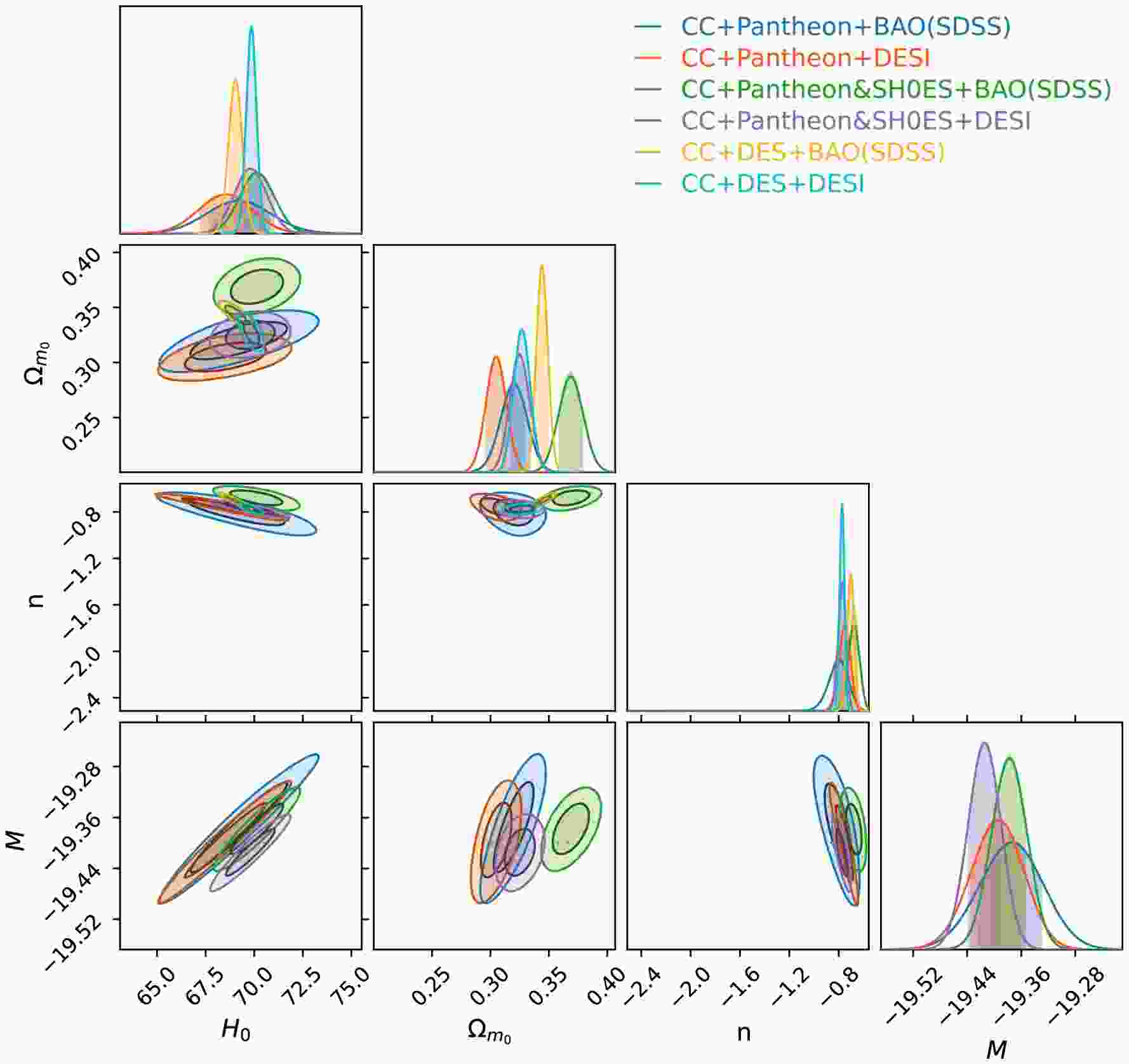
This system is nonlinear and cannot be solved analytically; therefore, numerical techniques are required for parameter estimation. The resulting parameter estimates are summarized in Table 1, and the corresponding confidence contours and posterior distributions are shown in Fig. 1. In the limit $ \alpha \to 0 $, the model reduces to standard GR, thereby recovering the ΛCDM behavior.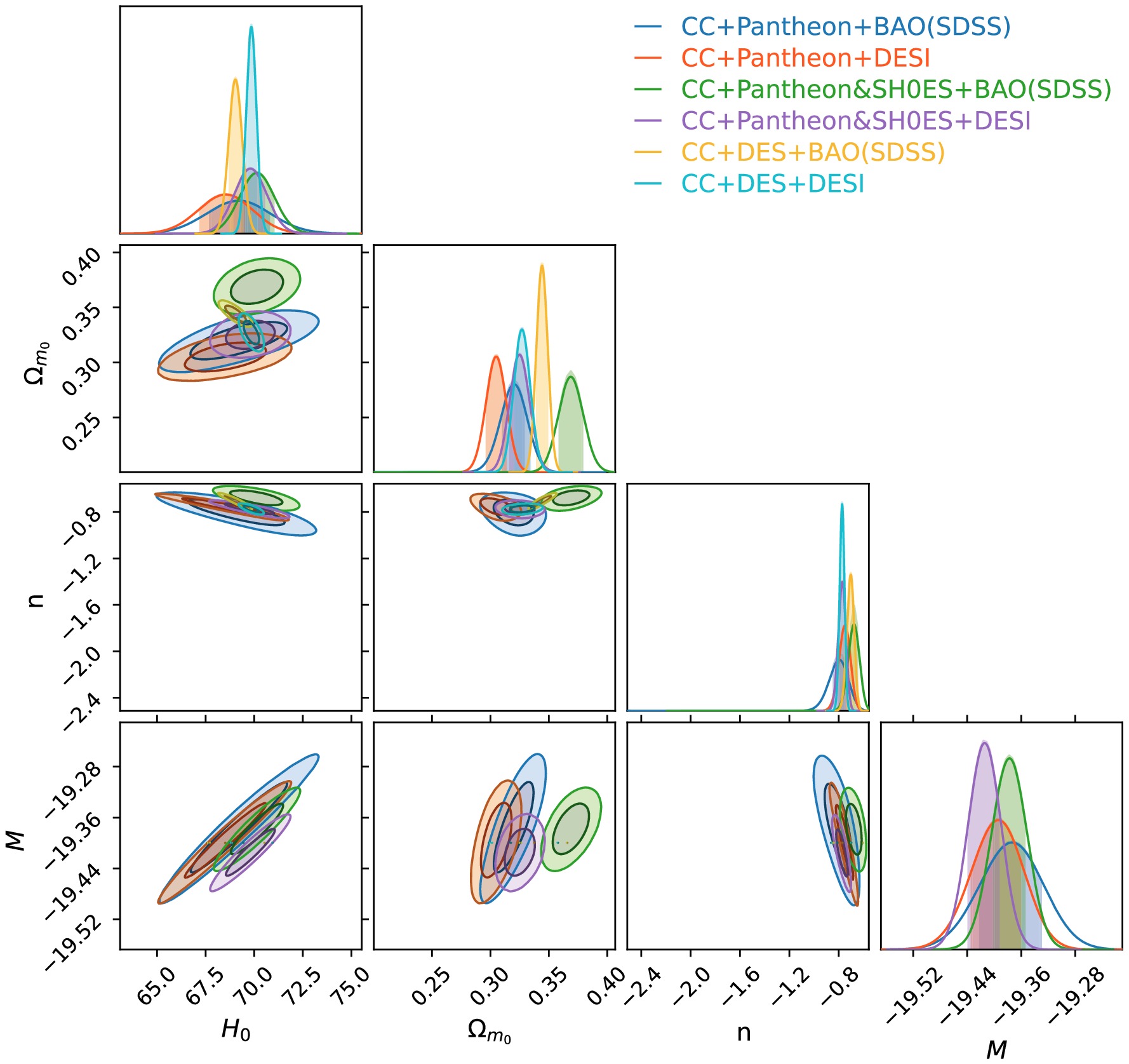

Figure 1.  (color online) Contour plot of the combined dataset comprising CC, Pantheon, Pantheon+SHOES, BAO (SDSS), and DESI for Model I.

For the dataset combination CC+PN+SDSS, the Hubble constant is constrained to $ H_0 = 69.2^{+1.6}_{-1.7}\ {\rm{km}}\ {\rm{s}}^{-1}\ {\rm{Mpc}}^{-1} $, with $ \Omega_{m,0} = 0.320 \pm 0.011 $ and $ n = -0.792^{+0.069}_{-0.079} $. Replacing SDSS with DESI (CC+PN+DESI) slightly shifts the central value to $ H_0 = 68.5 \pm 1.4 $ and yields tighter constraints on $ \Omega_{m,0} $ and n, reflecting the improved precision of the DESI measurements. This trend is also evident in the posterior distributions in Fig. 2, where the DESI-based histogram is narrower than the corresponding SDSS result, indicating reduced parameter uncertainties.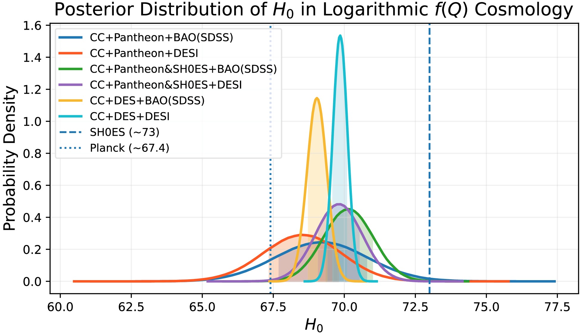

Figure 2.  (color online) Posterior probability distributions of the Hubble constant $ H_0 $ for Model I, obtained from different combinations of observational datasets.

When the PN(SH0ES) dataset is included, the inferred value of the Hubble constant increases, as expected from the Cepheid calibration. Specifically, for CC+PN(SH0ES)+SDSS, we obtain $ H_0 = 70.15^{+0.87}_{-0.89} $, whereas the CC+PN(SH0ES)+DESI combination yields $ H_0 = 69.80^{+0.84}_{-0.81} $. In both cases, the uncertainties are reduced compared with the Pantheon-only results, and the parameter n shifts toward less negative values, indicating a mild dependence of the model dynamics on the choice of supernova dataset. In the histogram panel, these combinations produce posterior peaks shifted toward higher values of $ H_0 $, bringing the results closer to the SH0ES local measurement.

A more substantial tightening of the constraints is observed when the DES SN5YR dataset is employed. For CC+DES+SDSS, the Hubble constant is constrained to $ H_0 = 69.04 \pm 0.35 $, while for CC+DES+DESI, it becomes $ H_0 = 69.85 \pm 0.26 $. The corresponding values of $ \Omega_{m,0} $ and n are also tightly constrained, with uncertainties significantly smaller than those obtained from Pantheon-based datasets. This improvement is primarily due to the larger sample size and reduced systematic uncertainties of the DES SN5YR dataset. The posterior distributions are considerably sharper, demonstrating the strong constraining power of the DES SN5YR data. Across all dataset combinations, the matter density parameter $ \Omega_{m,0} $ remains within the range $ 0.30 $–$ 0.37 $, consistent with standard cosmological estimates. The model parameter n consistently takes negative values, typically around $ n \sim -0.7 $, indicating deviations from the ΛCDM limit while maintaining compatibility with observational data. Furthermore, the histogram distributions in Fig. 2 show that the inferred values of $ H_0 $ generally lie between the Planck and SH0ES measurements, suggesting that the model may provide a possible route toward alleviating the $ H_0 $ tension.

In Model II, we consider a nonlinear saturating form of $ \Phi(Q) $ designed to regulate higher-order contributions of the nonmetricity scalar and provide controlled evolution of the cosmological dynamics across different epochs. The functional form is given by

where the parameter n controls the strength and rate of the nonlinear saturation, while α determines the overall amplitude of the modification. The normalization constant α is determined by evaluating the modified Friedmann equation at the present epoch, yielding

This functional form is considered because it introduces a bounded nonlinear correction to the standard $ f(Q)=Q $ theory. In contrast to the logarithmic correction considered in Model I, the nonlinear structure of Model II suppresses the modification's relative contribution at large values of the nonmetricity scalar. This provides a complementary phenomenological realization in which late-time expansion can be modified, while the correction becomes progressively less important in the high-curvature regime. Thus, Model II allows us to investigate whether a saturating modification of the nonmetricity sector can provide a viable cosmological background while remaining close to standard gravitational behavior at sufficiently large Q.

For convenience, we introduce the dimensionless variable $ x=\frac{Q}{Q_0} $.

The modification can then be expressed as

and the full gravitational function is

The first derivative of $ f(Q) $ with respect to Q is

while the second derivative is

These derivatives are useful for analyzing the behavior of the gravitational sector and the stability of the cosmological solutions.

A necessary condition for maintaining the correct sign of the gravitational kinetic term is

For Model II, this condition can be written explicitly as

Consequently, the physically relevant cosmological solutions should remain within the region of parameter space in which $ f_Q $ remains positive and does not cross zero.

The asymptotic behavior of Model II can be examined by considering the low- and high-curvature limits. Since $ Q=6H^2 $, the limits $ Q\ll Q_0 $ and $ Q\gg Q_0 $ correspond to the low- and high-curvature regimes, respectively. For $ Q\ll Q_0 $, or $ x\ll1 $, the nonlinear term can be expanded as

Consequently,

or equivalently,

Hence,

and therefore

Furthermore,

which gives

Thus, the nonlinear saturation model has a regular low-curvature limit for both $ \Phi(Q) $ and $ f_Q $.

The high-curvature behavior is obtained by considering $ Q\gg Q_0 $, or equivalently $ x\gg1 $. In this regime,

In the observationally preferred region of Model II, $ n>0 $; therefore,

Consequently,

Although the modification tends to a finite constant, its contribution relative to the leading nonmetricity term vanishes:

Therefore,

and the leading-order behavior of the theory approaches

Because the additional term remains constant as Q increases, its relative effect on the gravitational dynamics becomes negligible. Moreover,

so that

for $ n>0 $. Similarly,

Thus, Model II has a regular high-curvature limit in which the modification becomes subdominant to the standard Q contribution.

The asymptotic properties of Model II therefore differ qualitatively from those of the logarithmic Model I. In Model I, the favored negative values of n suppress the relative correction at high curvature but can lead to a singular derivative structure in the formal $ Q\rightarrow0 $ limit. In contrast, Model II is constructed so that $ \Phi(Q) $ vanishes quadratically near $ Q=0 $ and approaches a finite constant at large Q. Consequently, the nonlinear saturation form provides a more regular interpolation between the low- and high-curvature regimes.

The positivity condition $ f_Q>0 $ provides an important necessary viability criterion for Model II. Using the observationally constrained parameters, this condition can be evaluated along the corresponding cosmological background solutions. In particular, the observational analysis yields positive values of n for all dataset combinations considered, with the preferred value approaching zero when the more precise DES and DESI data are included. This behavior indicates that the nonlinear modification becomes progressively weaker for the most tightly constrained dataset combinations.

However, the condition $ f_Q>0 $ is a necessary gravitational-sector viability condition and does not, by itself, establish complete perturbative ghost freedom. A complete stability analysis requires expanding the action to second order in scalar, vector, and tensor perturbations and examining the corresponding kinetic and gradient terms. In particular, the absence of ghost instabilities requires positive kinetic coefficients, while the absence of gradient instabilities requires non-negative squared propagation speeds. Therefore, the present analysis establishes the background asymptotic behavior and the basic condition $ f_Q>0 $, but it does not constitute a complete proof of ghost-free perturbative stability.

The nonlinear saturation form nevertheless has a theoretically desirable feature: both the $ Q\rightarrow0 $ and $ Q\rightarrow \infty $ limits remain regular at the level of $ \Phi(Q) $ and $ f_Q $, with the latter approaching the standard value $ f_Q=1 $. A complete scalar-, vector-, and tensor-perturbation analysis, including the explicit ghost and gradient-stability conditions, is beyond the scope of the present background-level observational study and will be considered in future work.

The evolution equation for the normalized Hubble parameter $ E(z)=H(z)/H_0 $ takes the form

which, similar to Model I, is nonlinear and must be solved numerically. This formulation effectively suppresses large deviations at high redshift while allowing controlled modifications at late cosmic times.

The constraints on the model parameters derived from various combinations of observational datasets are presented in Table 2, and the corresponding confidence contours are shown in Fig. 3. These datasets include CC, Type Ia supernovae (Pantheon, Pantheon+SH0ES, and DES SN5YR), and BAO measurements from SDSS and DESI. The contour plots illustrate the correlations among the cosmological parameters $ (H_0,\Omega_{m,0},n) $ and show that the allowed parameter space becomes progressively more constrained with the inclusion of more precise datasets, particularly DESI observations.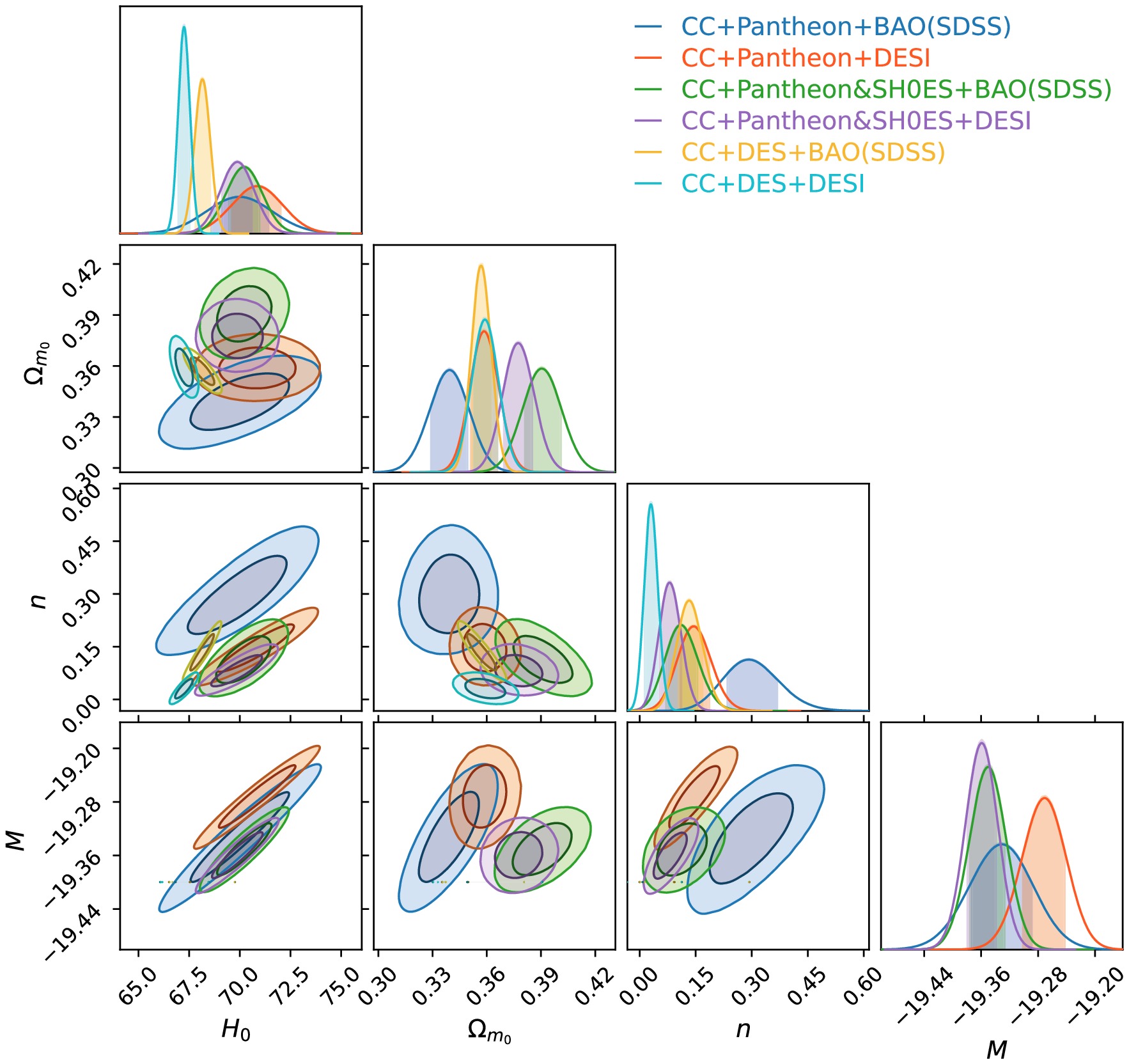

Figure 3.  (color online) Contour plot for the combined CC, Pantheon, Pantheon+SHOES, BAO(SDSS), and DESI datasets for Model-II.

For the CC+PN+SDSS combination, the Hubble constant is constrained to be $ H_0 = 70.0 \pm 1.6\ {\rm{km}}\ {\rm{s}}^{-1}\ {\rm{Mpc}}^{-1} $, with $ \Omega_{m,0} = 0.340 \pm 0.011 $ and $ n = 0.292^{+0.076}_{-0.071} $. The corresponding contours in Fig. 3 show relatively broad allowed regions, particularly in the $ (H_0,n) $ plane, indicating weaker constraints on the nonlinear parameter n. When DESI data are used instead (CC+PN+DESI), the value shifts to $ H_0 = 70.9^{+1.2}_{-1.3} $, accompanied by tighter constraints on $ \Omega_{m,0} $ and a noticeable decrease in the parameter n, reflecting the impact of higher-precision BAO measurements. This improvement is evident in Fig. 3, where the confidence regions shrink considerably compared with the SDSS case.

Including the PN(SH0ES) dataset leads to a moderate shift in the inferred parameters. For CC+PN(SH0ES)+SDSS, we obtain $ H_0 = 70.24^{+0.86}_{-0.91} $, whereas the CC+PN(SH0ES)+DESI combination yields $ H_0 = 69.88 \pm 0.83 $. In both cases, the uncertainties are reduced compared with the Pantheon-only combinations, and the parameter n decreases further, suggesting weaker deviations from the standard cosmological model when local calibration data are included.

To further examine the behavior of the Hubble constant in this model, the posterior distributions of $ H_0 $ for all dataset combinations are presented in Fig. 4. The figure shows that the Pantheon- and Pantheon+SH0ES-based combinations generally favor values around $ H_0 \sim 70\ {\rm{km}}\ {\rm{s}}^{-1}\ {\rm{Mpc}}^{-1} $, lying between the SH0ES and Planck reference measurements. This indicates that the nonlinear saturation $ f(Q) $ model naturally accommodates intermediate values of the Hubble constant and partially alleviates the tension between local and early-Universe observations.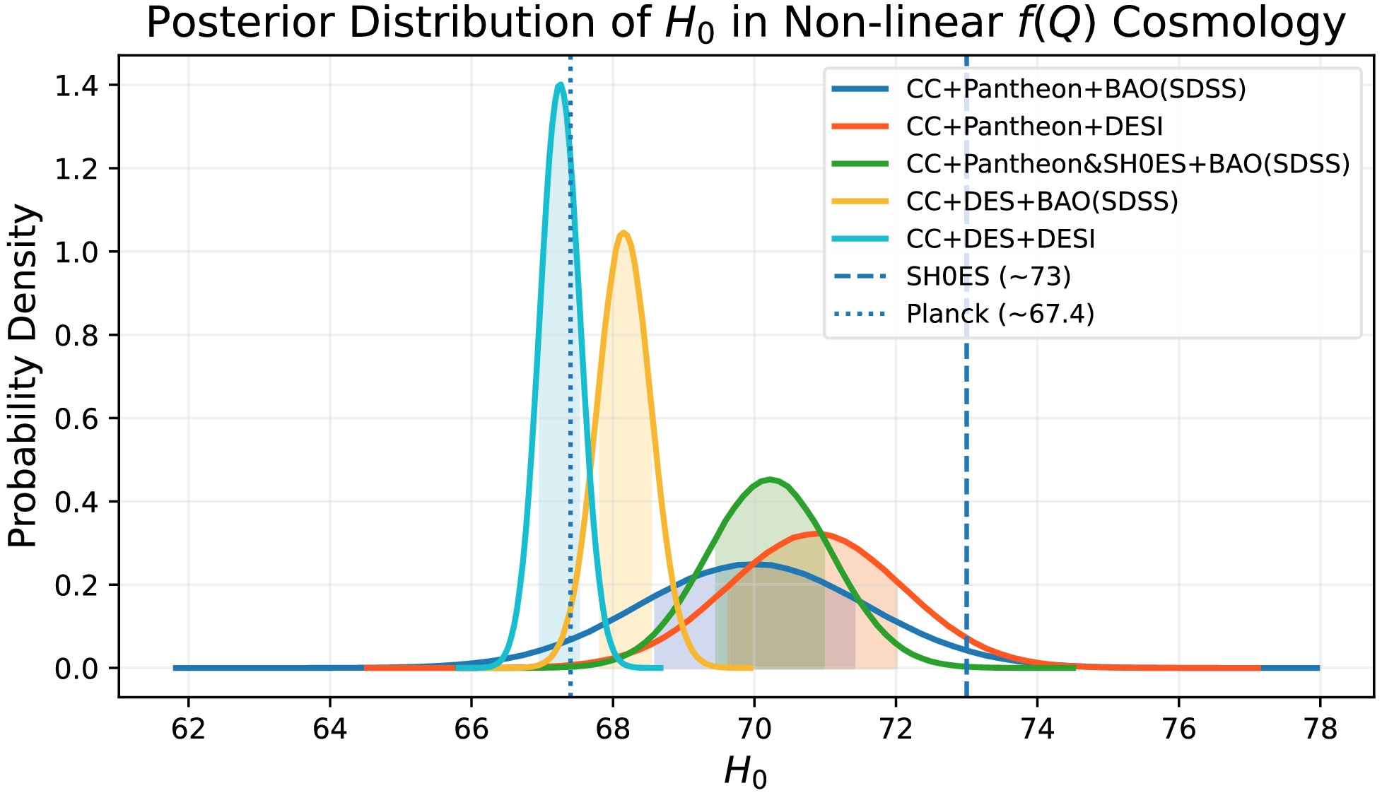

Figure 4.  (color online) Posterior probability distributions for the Hubble constant $ H_0 $ in Model II, obtained from different combinations of observational datasets.

A distinct behavior is observed when the DES SN5YR dataset is considered. For CC+DES+SDSS, the Hubble constant is constrained to $ H_0 = 68.15^{+0.39}_{-0.37} $, whereas CC+DES+DESI gives $ H_0 = 67.25^{+0.29}_{-0.28} $. These results provide significantly tighter constraints, particularly in the latter case, where the uncertainty in $ H_0 $ is reduced to below 0.5%. This trend is consistently reflected in both figures. In Fig. 3, the confidence contours become substantially smaller and more localized, while Fig. 4 shows that the DES-based datasets shift the posterior distributions toward lower values of $ H_0 $. This shift is especially pronounced for the CC+DES+DESI combination, whose peak lies close to the Planck measurement. Moreover, the CC+DES+DESI case produces the narrowest posterior distribution among all combinations, highlighting the strong constraining power of the combined DES and DESI observations.

The matter density parameter $ \Omega_{m,0} $ remains tightly constrained across all dataset combinations, generally favoring slightly higher values than Model I, typically in the range $ 0.34 $–$ 0.39 $. The contour structure in Fig. 3 further indicates a mild correlation between $ \Omega_{m,0} $ and n, with smaller values of n associated with slightly larger matter densities. The model parameter n is consistently positive in this case, with values decreasing from $ \sim 0.3 $ for Pantheon-based datasets to $ \sim 0.03 $ for the CC+DES+DESI combination. This behavior suggests that the inclusion of increasingly precise observational data systematically drives the nonlinear saturation $ f(Q) $ model closer to the ΛCDM limit, corresponding to smaller deviations from standard cosmology.

A direct comparison of Model I (logarithmic) and Model II (nonlinear saturation) reveals both the robustness of the inferred cosmological parameters and their sensitivity to dataset choice across two distinct functional forms of $ f(Q) $ gravity. Fig. 5 displays the estimated values of $ H_0 $ at the three vertices corresponding to Model I, Model II, and ΛCDM for all six dataset combinations. The overall compactness of the polygon formed by each dataset trace indicates that the two modified gravity models and ΛCDM occupy largely overlapping regions of parameter space with respect to $ H_0 $. For the CC+PN+SDSS combination, Model I yields $ H_0 = 69.2^{+1.6}_{-1.7} $ km s⁻¹ Mpc⁻¹, whereas Model II yields $ H_0 = 70.0 \pm 1.6 $ km s⁻¹ Mpc⁻¹, a difference well within the $ 1\sigma $ uncertainties. Similarly, for CC+PN+DESI, Model I gives $ H_0 = 68.5 \pm 1.4 $, whereas Model II gives $ H_0 = 70.9^{+1.2}_{-1.3} $. Across these baseline combinations, Model I consistently returns $ H_0 $ values closer to the intermediate range between the Planck CMB and SH0ES distance-ladder results, whereas Model II exhibits slightly greater scatter. This suggests that the logarithmic correction provides a more stable geometric response to the underlying data.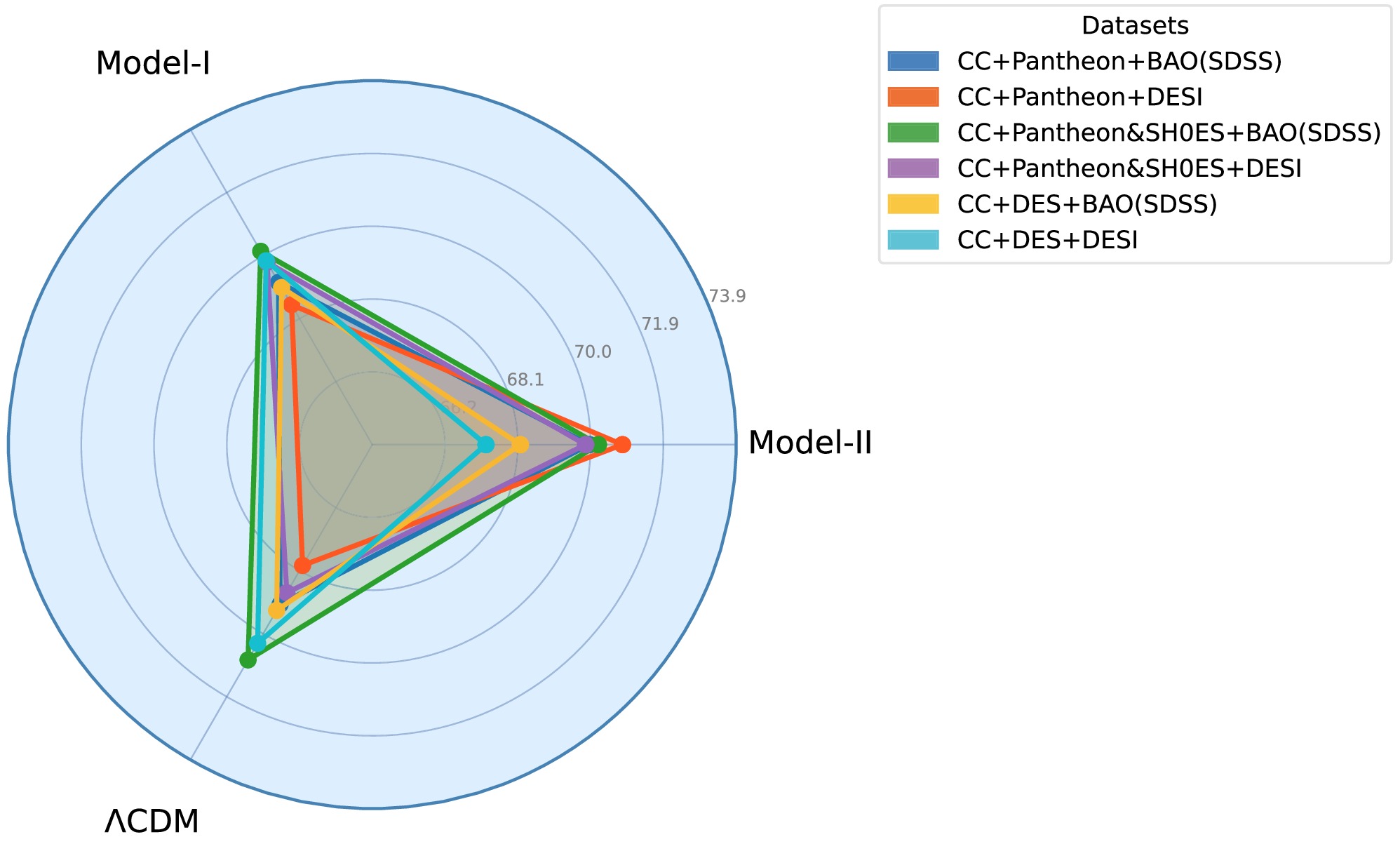

Figure 5.  (color online) The plot illustrates the inferred $ H_0 $ values (in km s⁻¹ Mpc⁻¹) for Model I, Model II, and ΛCDM across six dataset combinations; the radial scale ranges from $ 66.2 $ to $ 73.9 $ km s⁻¹ Mpc⁻¹.

When the PN(SH0ES) dataset is incorporated, both models exhibit a systematic upward shift in the inferred $ H_0 $, regardless of the BAO counterpart used. For CC+PN(SH0ES)+DESI, Model I gives $ H_0 = 69.80^{+0.84}_{-0.81} $, and Model II gives $ H_0 = 69.88 \pm 0.83 $, in near-perfect agreement. Likewise, for CC+PN(SH0ES)+SDSS, the values are $ H_0 \approx 70.15 $ (Model I) and $ H_0 \approx 70.24 $ (Model II). This behavior is clearly captured in the radar plot by the green trace (CC+Pantheon&SH0ES+BAO(SDSS)), which consistently extends to the outermost ring near $ 73.9 $ at the Model I vertex – the largest $ H_0 $ excursion recorded across the entire comparison. These findings confirm that SH0ES calibration systematically drives $ H_0 $ upward independently of the underlying gravity model, indicating that the observational calibration is the dominant source of this shift.

The DES SN5YR dataset imposes the tightest constraints in both models, as indicated by the clustering of the yellow (CC+DES+SDSS) and cyan (CC+DES+DESI) traces near the center of the radar plot and by their substantially reduced uncertainties. For CC+DES+DESI, Model I yields $ H_0 = 69.85 \pm 0.26 $, whereas Model II gives $ H_0 = 67.25^{+0.29}_{-0.28} $ km s⁻¹ Mpc⁻¹. The central values differ by approximately $ 2.6 $ km s⁻¹ Mpc⁻¹, yet both have sub-percent uncertainties. Here, the distinction between the two models is most pronounced: Model I returns $ H_0 = 69.85 \pm 0.26 $, which remains well within the intermediate range that can ease the tension, whereas Model II yields $ H_0 = 67.25^{+0.29}_{-0.28} $, which lies closer to the Planck estimate and therefore provides less leverage in addressing the Hubble tension. Similarly, for CC+DES+SDSS, Model I gives $ H_0 = 69.04 \pm 0.35 $, compared with $ H_0 = 68.15^{+0.39}_{-0.37} $ from Model II, reinforcing the same trend. This systematic difference indicates that the logarithmic functional form of Model I, owing to its unbounded growth at large nonmetricity, is better able than the saturating correction of Model II to sustain $ H_0 $ at values capable of partially alleviating the tension with local distance-ladder measurements.

In Model I, n controls the power-law dependence of the logarithmic nonmetricity correction on the scale $ Q/Q_0 $. The preferred value, $ n\simeq-0.7 $, implies that the relative contribution of the modification is suppressed at high curvature while allowing a scale-dependent modification at late times. In Model II, n controls the rate of nonlinear saturation of the correction. For $ n>0 $, the modification approaches a finite value at high Q, whereas $ n=0 $ gives $ \Phi(Q)=0 $ and recovers the standard $ f(Q)=Q $ limit. The preferred value decreases from approximately $ n\simeq0.3 $ for the CC+PN+SDSS combination toward $ n\simeq0 $ for the combinations involving DES and DESI, indicating a progressively weaker nonlinear modification.

The prior range of n was chosen to be sufficiently broad to encompass the relevant modified-gravity behavior and was fixed independently of the observational results. We adopted a flat prior, and the MCMC analysis explored the entire adopted prior interval rather than being restricted to the region favored by the data. Thus, the posterior constraints on n are determined by the observational likelihood rather than imposed by the prior choice. Regions outside the adopted prior interval were not considered in the present analysis.

To quantify the extent to which the proposed models alleviate the Hubble tension, we calculate the tension between the inferred $H_0$ values and the Planck and SH0ES determinations. The tension is defined as

For the quoted Planck and SH0ES measurements, the corresponding discrepancy is $4.68\sigma$. The resulting tension values for the two $f(Q)$ models are presented in Table 3. Model I reduces the discrepancy with SH0ES to approximately $2.0$–$3.7\sigma$ for the dataset combinations considered. Model II shows stronger alleviation for some combinations, with the tension reaching as low as $1.35\sigma$ for the CC+PN+DESI dataset. However, the tension remains dataset dependent, and some combinations yield a substantially larger discrepancy with SH0ES. These results indicate that the proposed $f(Q)$ models can partially alleviate the Hubble tension.

The ΔAIC and ΔBIC values presented in Tables 1 and 2, and visualised in Fig. 6, statistically reinforce this conclusion. For Model I, ΔAIC ranges from a minimum of 0.20 (CC+PN+SDSS) to a maximum of 3.83 (CC+PN(SH0ES)+DESI), with the corresponding ΔBIC values spanning 5.19 to 9.29. According to the Jeffreys scale, ΔAIC < 2 implies substantial support relative to the reference model, while $ 2 \lt \Delta $AIC < 4 indicates a positive but weaker preference. Model I has substantial statistical support from the CC+PN+SDSS and CC+PN(SH0ES)+SDSS combinations and positive support from the remaining combinations, establishing it as a statistically viable alternative to ΛCDM across the full range of datasets considered. For Model II, ΔAIC ranges from 0.88 (CC+DES+SDSS) to 4.34 (CC+PN(SH0ES)+DESI), with ΔBIC spanning 6.41 to 9.80. Although Model II achieves a lower ΔAIC $ = 0.88 $ than Model I (1.60) for CC+DES+SDSS – visible as a crossing of the two AIC lines at dataset index 4 in Fig. 6 – this advantage occurs precisely for the configuration in which Model II yields a lower $ H_0 $, offering less capacity to ease the Hubble tension. For CC+PN(SH0ES)+DESI (dataset index 3), both models reach their largest information-criterion differences (ΔAIC $ = 3.83 $ and $ 4.34 $; ΔBIC $ = 9.29 $ and $ 9.80 $ for Models I and II, respectively), with Model I retaining the smaller penalty throughout. The BIC curves lie systematically above the AIC curves for both models across all dataset combinations, reflecting the expected large-n penalty, while the two models closely track each other in their information-criterion profiles. We also consider the Deviance Information Criterion (DIC), which accounts for both goodness of fit and the effective complexity of the model. The ΔDIC values for Model I range from 0.15 to 3.75, whereas those for Model II range from 0.67 to 4.12. Model I yields the smallest ΔDIC for CC+PN+SDSS ($ \Delta {\rm{DIC}}=0.15 $) and remains below 2 for the CC+PN+SDSS, CC+PN+DESI, CC+PN(SH0ES)+SDSS, CC+DES+SDSS, and CC+DES+DESI combinations, indicating a comparatively small DIC difference relative to ΛCDM. Model II also shows competitive DIC values for CC+PN+SDSS and CC+DES+SDSS, with $ \Delta {\rm{DIC}}=2.21 $ and 0.67, respectively, but reaches its largest difference of 4.12 for CC+PN(SH0ES)+DESI. Taken together, the AIC, BIC, and DIC results show that Model I is generally more competitive with ΛCDM than Model II across the considered dataset combinations. In particular, Model I simultaneously provides relatively small information-criterion differences and higher $ H_0 $ values for most datasets, making the logarithmic correction a more consistent candidate for partially alleviating the Hubble tension. Nevertheless, the statistical preference remains dataset dependent, and neither model is strongly preferred over ΛCDM for all observational combinations.

Figure 6.  (color online) Variations in ΔAIC and ΔBIC for Model I and Model II relative to ΛCDM across six dataset combinations. Solid and dashed lines represent ΔAIC and ΔBIC, respectively.

In this work, we investigated the cosmological implications of two representative $ f(Q) $ gravity models within the framework of symmetric teleparallel gravity using a comprehensive set of late-time observational datasets, including CC, Type Ia supernova compilations (Pantheon, Pantheon+SH0ES, and DES SN5YR), and baryon acoustic oscillation (BAO) measurements from SDSS and DESI.

For the logarithmic Model-I, the inferred values of the Hubble constant generally lie in the range $ H_0 \sim 68.5 $ – $ 70.2\; {\rm{km}}\ {\rm{s}}^{-1}\ {\rm{Mpc}}^{-1} $, depending on the adopted dataset combination. In particular, the inclusion of the Pantheon+SH0ES compilation systematically shifts the preferred value of $ H_0 $ toward higher values, bringing the results closer to the local SH0ES determination. The DESI datasets substantially improve the precision of the constraints compared with SDSS, producing narrower confidence contours and posterior distributions. Moreover, the DES SN5YR dataset yields the tightest parameter constraints, with uncertainties reduced to subpercent levels in some combinations. Across all datasets, the model parameter n remains negative, indicating deviations from the ΛCDM limit while maintaining consistency with cosmological observations. Importantly, the posterior distributions show that the logarithmic correction naturally favors intermediate values of $ H_0 $ between the Planck and SH0ES measurements, suggesting that Model-I can partially alleviate the Hubble tension.

For the nonlinear saturation Model-II, the cosmological constraints exhibit somewhat different behavior. The Pantheon and Pantheon+SH0ES combinations again favor values around $ H_0 \sim 70\; {\rm{km}}\ {\rm{s}}^{-1}\ {\rm{Mpc}}^{-1} $, but the inclusion of DES and DESI data systematically drives the inferred Hubble constant toward lower values closer to the Planck estimate. In particular, the CC+DES+DESI combination yields $ H_0 = 67.25^{+0.29}_{-0.28}\; {\rm{km}}\ {\rm{s}}^{-1}\ {\rm{Mpc}}^{-1} $, which is strongly consistent with early-Universe measurements but less effective in addressing the local Hubble tension. The nonlinear parameter n remains positive and gradually approaches zero as the datasets become more precise, indicating that the model tends toward the ΛCDM limit when confronted with stronger observational constraints. This behavior suggests that the saturation mechanism suppresses large deviations from standard cosmology at late times.

A direct comparison of the two models shows that Model-I generally provides a more favorable framework for easing the Hubble tension. The logarithmic correction consistently predicts intermediate values of $ H_0 $ that remain statistically compatible with both early- and late-Universe measurements, whereas Model-II tends to converge toward the lower values favored by Planck. This distinction becomes especially pronounced for the DES+DESI combinations, for which Model-I retains $ H_0 $ values near $ 70\; {\rm{km}}\ {\rm{s}}^{-1}\ {\rm{Mpc}}^{-1} $, while Model-II approaches the standard ΛCDM prediction. These results indicate that the logarithmic form of the nonmetricity correction introduces a more flexible late-time expansion history capable of sustaining larger Hubble values without significantly degrading the fit to observational data.

The statistical comparison based on the AIC, BIC, and DIC further supports these conclusions. Both models remain statistically competitive with the ΛCDM cosmology, with relatively small values of $ \Delta {\rm{AIC}} $, $ \Delta {\rm{BIC}} $, and $ \Delta {\rm{DIC}} $ across all dataset combinations. However, Model-I generally exhibits lower information-criterion differences than Model-II, particularly for the Pantheon-based datasets, indicating a better balance between model complexity and goodness of fit. Although Model-II performs slightly better for the CC+DES+SDSS combination, this occurs precisely in the regime where the inferred value of $ H_0 $ shifts closer to the Planck estimate, reducing its effectiveness in addressing the Hubble tension.

For completeness, we also analyzed the standard ΛCDM model using the same observational datasets. The results show that the inferred value of $ H_0 $ remains highly sensitive to the adopted late-time observations. Pantheon-only combinations yield values close to the Planck estimate, whereas Pantheon+SH0ES combinations shift the preferred $ H_0 $ upward toward the local SH0ES measurement. DESI data consistently provide tighter constraints than SDSS, highlighting the increasing precision of recent BAO observations. Overall, the ΛCDM framework continues to provide an excellent fit to the available data, although the dependence of $ H_0 $ on dataset selection demonstrates that the Hubble tension remains unresolved within the standard cosmological scenario.

In summary, the two $f(Q)$ models provide viable descriptions of the observed late-time expansion history while exhibiting distinct effects on the inferred value of $H_0$. The logarithmic model shows a comparatively stronger tendency to shift the inferred $H_0$ toward the local SH0ES measurement, whereas the nonlinear model provides a consistent fit with a weaker departure from the standard $f(Q)=Q$ behavior for some dataset combinations. These results indicate that modifications of the nonmetricity sector can influence the late-time expansion rate and, consequently, affect the value of the Hubble constant inferred from cosmological observations. The statistical analysis further shows that the relative performance of the two models depends on the dataset combination, reflecting the complementary constraining power of the different observational probes. In particular, the inclusion of recent BAO measurements provides additional constraints on the expansion history and helps distinguish between the different functional forms of $f(Q)$. The combined observational results therefore support the viability of these models as phenomenological alternatives to $\Lambda$CDM, while also indicating that their ability to alleviate the $H_0$ tension is insufficient to claim a complete resolution. The logarithmic model appears particularly promising in this respect, as it provides closer agreement with the local determination of $H_0$ while maintaining compatibility with the considered cosmological datasets. Further improvements in observational precision will be important for determining whether this preference persists and whether modified late-time dynamics are genuinely required.

BM acknowledges IUCAA, Pune (India), for support during an academic visit, during which part of this work was completed. The authors thank the referees for their constructive comments and suggestions, which helped improve the paper.

The parameter constraints for the ΛCDM model derived from different combinations of the CC, Pantheon/Pantheon+SH0ES, DES, SDSS, and DESI datasets are summarized in Table 4. The analysis shows that the estimated value of the Hubble constant, $ H_0 $, depends sensitively on the choice of observational datasets. For combinations including Pantheon and BAO data, the inferred values of $ H_0 $ lie in the range $ 67.9 $–$ 69.1\; {\rm{km}}\ {\rm{s}}^{-1}\ {\rm{Mpc}}^{-1} $, remaining broadly consistent with the $ Planck $ CMB estimate. In contrast, including the Pantheon+SH0ES compilation shifts the preferred value of $ H_0 $ toward higher values, reaching $ 70.81 \pm 0.72\; {\rm{km}}\ {\rm{s}}^{-1}\ {\rm{Mpc}}^{-1} $ for the CC+PN(SH0ES)+SDSS dataset combination and thereby reducing the tension with the local SH0ES measurement.

The matter density parameter $ \Omega_{m,0} $ is tightly constrained for all dataset combinations, with values in the range $ \Omega_{m,0}\sim0.28 $–$ 0.36 $. In particular, the DESI combinations provide significantly tighter bounds than the SDSS datasets, indicating the improved constraining power of the recent DESI BAO measurements. The absolute magnitude parameter M is also well constrained in the Pantheon-based analyses, with best-fit values around $ M\approx -19.4 $.

The minimum chi-square values and the corresponding information criteria (AIC, BIC, and DIC) indicate that all dataset combinations provide statistically acceptable fits within the ΛCDM framework. However, the DESI datasets generally yield slightly lower information-criterion values than the SDSS datasets, suggesting marginally better consistency with the ΛCDM cosmology. Overall, the results demonstrate that the standard ΛCDM model continues to provide an excellent description of current cosmological observations, while the inferred value of $ H_0 $ still exhibits a noticeable dependence on the adopted late-time datasets (Fig. 7).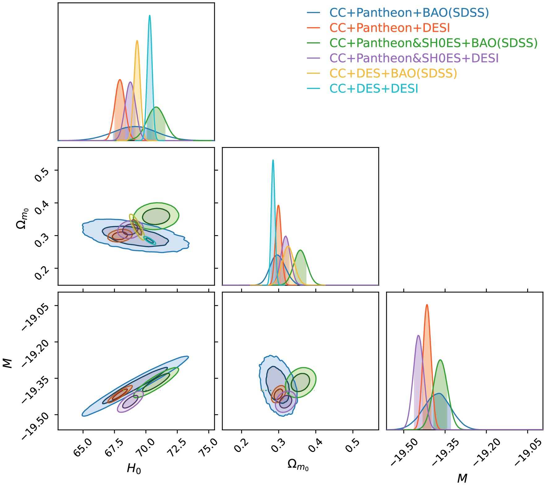

Figure 7.  (color online) Contour plot for the combined CC, Pantheon, Pantheon+SH0ES, BAO(SDSS), and DESI data sets under ΛCDM.

The posterior distributions further illustrate the dataset dependence of $ H_0 $ (Fig. 8). The Pantheon+SH0ES combinations favor higher values of the Hubble constant, closer to the SH0ES estimate ($ \sim73\; {\rm{km}}\ {\rm{s}}^{-1}\ {\rm{Mpc}}^{-1} $), whereas the Pantheon and DES-based combinations remain closer to the $ Planck $ prediction ($ \sim67.4\; {\rm{km}}\ {\rm{s}}^{-1}\ {\rm{Mpc}}^{-1} $). Similarly, the combined contour plots show correlations among $ H_0 $, $ \Omega_{m,0} $, and M, indicating that DESI data yield narrower confidence contours and therefore tighter cosmological parameter constraints.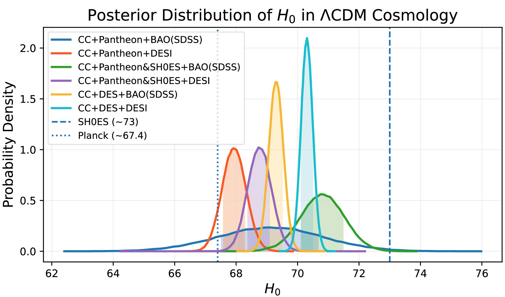

Figure 8.  (color online) Posterior probability distributions of the Hubble constant, $ H_0 $, for the ΛCDM model, obtained from different combinations of observational datasets.