Schwinger current in de Sitter space

A strong electric field is expected to produce electron-positron pairs out of the quantum field theory (QFT) vacuum. This phenomenon was first hinted at in 1936 by Euler and Heisenberg [1], remarkably long before the development of our modern theory of Quantum Electrodynamics (QED), and was then firmly predicted in a seminal paper by Schwinger [2]. Today, the effect is known as Schwinger pair production, but it has yet to be observed in the laboratory ¹. This puts us in the fascinating situation in which one of the fundamental predictions of QED, possibly our most successful theory of nature, has yet to be tested experimentally. The primary reason is that an intense electric field is required, of the order of the electron mass squared. This is still beyond current technology, but there is hope that this phenomenon will be observed in the laboratory in the not-too-distant future [6, 7].

These technological challenges on Earth could potentially be overcome in the early Universe during inflation, when enormous amounts of energy were available to generate strong electric fields. Furthermore, as we examine in detail, in an expanding spacetime, the Schwinger effect can occur even with very weak electric fields. Mechanisms for generating the necessary constant electric field during inflation can be easily constructed by coupling a $ U(1) $ gauge field to the expanding spacetime [8−13]. This raises the interesting possibility that the first experimental observation of the Schwinger effect could come from cosmological signals [14].

The Schwinger current in de Sitter space was first computed in 1+1 dimensions [15] and then in 3+1 dimensions for minimally coupled spin-0 [16−18] and spin-1/2 [19] charged particles. The current is formally divergent but, remarkably, can be obtained analytically and non-perturbatively, and made finite by using an appropriate renormalization procedure. In 3+1 dimensions, both the scalar and fermion currents were found to have a peculiar negative IR divergence in the small electron ² mass limit. This implies not only a divergent current but also one that flows in the direction opposite to the electric field. Understanding this seemingly unphysical behavior is not just an academic curiosity; it can have important implications for primordial magnetogenesis [16] and play a role in the production of dark matter [20−22].

In this work, we argue that the appearance of these IR divergences is due to the renormalization procedures implicitly used in [16−18]. Imposing physical renormalization conditions that are consistent with a constant electric field in de Sitter space, we show that the renormalized current is free of UV and IR divergences, both for scalars and fermions. In deciding how to fix the renormalization conditions, we first point out that, in order to sustain a constant electric field in de Sitter space, a tachyonic instability is unavoidable. Requiring the electric field to be constant and uniform both inside and outside the Hubble horizon, as was assumed in [16−18], implies that the photon, treated as a classical dynamical field, must have a tachyonic mass $ m_A^2 = -2H^2 $, where H is the Hubble constant. As we will show, the tachyonic mass condition leads to a modified on-shell renormalization condition that gives an IR-finite renormalized current. More details of our analysis can be found in an accompanying paper [23].

Here, as in previous studies of the Schwinger current [16, 18, 19], we consider a classical constant electric field in de Sitter space that is already present during inflation, and treat the spacetime geometry as a background. This means that we do not consider the dynamics of the energy-momentum tensor and do not address the renormalization of the vacuum energy. Crucially, and in contrast to previous works, we treat the classical gauge field $ A_\mu $, which is responsible for generating the constant electric field, as dynamical. This is because the only divergence in the theory, associated with the normalization of the photon field, is encoded in the vacuum polarization diagram [23], consisting of an electron loop with two external photon legs. To remove this divergence, we need the counterterm associated with such a diagram. This requires the two-point function of the photon field, which is obtained by treating the field dynamically.

We begin with the action for a free abelian gauge theory in a de Sitter spacetime background

Here, the metric is $ g_{\mu\nu} = a^2(\tau)(-{\rm{d}}\tau^2 + {\rm{d}}\vec x^2) $, with the conformal time denoted by τ

where $ F_{\mu\nu} = \partial_\mu A_\nu - \partial_\nu A_\mu $. We are interested in the configuration that realizes a constant, uniform electric field. For a comoving observer with 4-velocity $ u^\mu $ ($ u^i = 0 $, $ u_\mu u^\mu = -1 $), this electric field is given by $ E_\mu = u^\nu F_{\mu\nu} $, with field strength satisfying $ E_\mu E^\mu = E^2 = {\rm{const}} $. The gauge field configuration that produces such a constant electric field in de Sitter space along the z direction is given by [16, 18, 19]

Throughout this work, as in previous literature, we treat the gauge field as classical. However, as discussed above and unlike in previous literature, we treat it as dynamical rather than as a background, requiring it to solve the equation of motion

It is straightforward to check that Eq. (3) does not satisfy Eq. (4):

The simplest way to satisfy the equation of motion is to introduce a tachyonic mass

into the action for the gauge field

The photon mass $ m_A $ should be regarded as a Stueckelberg mass [24], obtained upon the replacement $ \dfrac{1}{2} m_A^2 A_\mu^2 \to \dfrac{1}{2} m_A^2 \left( A_\mu + \dfrac{1}{m_A} \partial_\mu \sigma \right)^2 $, where σ is the Stueckelberg field, and by adding the gauge-fixing term $ {\cal L}_{\rm{gf}} = - \sqrt{-g} \dfrac{1}{2\xi_A} \times \left( \partial_\mu A^\mu - \xi_A m_A \sigma \right)^2 $. The theory is then gauge invariant. We see that, in order to have a constant electric field in de Sitter space, we need a source term that breaks conformal invariance and provides a tachyonic condition, which is necessary to compensate for the exponential expansion of space.

A second possible solution is to introduce instead a modified kinetic term of the form $ (\tau_e/\tau) F_{\mu\nu} F^{\mu\nu} $, where $ \tau_e $ is a constant that could, for example, be fixed as the time at the end of inflation. As we show in Appendix A of [23], this leads to the same equations of motion as introducing a tachyonic mass with a canonically normalized kinetic term. In both scenarios, the electric field originates from a transverse component of the gauge field, which we treat as purely classical, with no contribution from the longitudinal mode. It should not be surprising that in de Sitter space the photon must have a tachyonic mass since, as space expands exponentially, the electric field must be continuously fed exponentially, meaning that a tachyonic instability is required to maintain a constant electric field. We will see below the crucial role that the tachyonic condition $ m_A^2 = -2H^2 $ plays in renormalization and in obtaining a physically consistent Schwinger current.

Since we are interested in computing the current of charged particles generated from the vacuum by the constant electric field, one might worry about radiative effects, which would require quantizing the photon field. However, shortly after they are produced, the charged particles reach terminal velocity [22], implying that the current very quickly reaches a constant value. We can therefore neglect radiative effects and solve the theory exactly by quantizing only the electron field, further justifying our classical treatment of the electric field.

We can write the renormalized Lagrangian in de Sitter space for a classical massive photon coupled to a current

All fields and parameters are understood to be renormalized, and the conserved current $ J^\mu $, which depends on the gauge coupling e, may describe either fermions or scalars. One can show [25] that the renormalized photon mass $ m_A $ is related to the bare mass by $ m_A^2 = (1- \delta_3)m_{A_0}^2 $, in the same way that the renormalized charge e is related to the bare charge, $ e^2 = (1-\delta_3) e^2_0 $, so there is no additional divergence. The counterterm $ \delta_3 $ is used to cancel the logarithmic divergence in the photon field normalization.

To define our theory, we must first fix the counterterm using an appropriate physical renormalization condition. Since the field $ A_\mu $ is classical, the obvious choice is to impose on-shell renormalization conditions. This requires the renormalized two-point function to have a pole at $ p^2 = -m_A^2 $ with residue $-{\rm i} $, which fixes

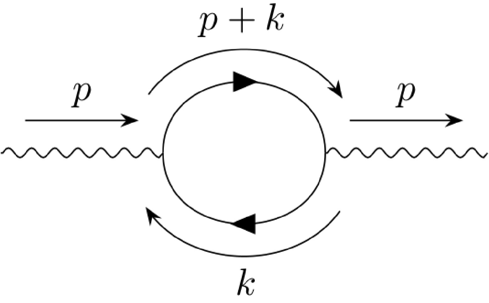
where $ e^2\Pi(p^2) $ is defined as the coefficient of $-{\rm i}\left(p^2 g^{\mu \nu} - p^\mu p^\nu\right)$ in the sum of all 1PI contributions to the photon two-point correlation function [26]. Since we have a classical electric field and $ A_\mu $ is not quantized, $ \Pi(p^2) $ is determined exactly at one loop, with the corresponding diagram shown in Fig. 1 (with a second diagram for scalars). This renormalization condition leads to the following condition on the counterterm: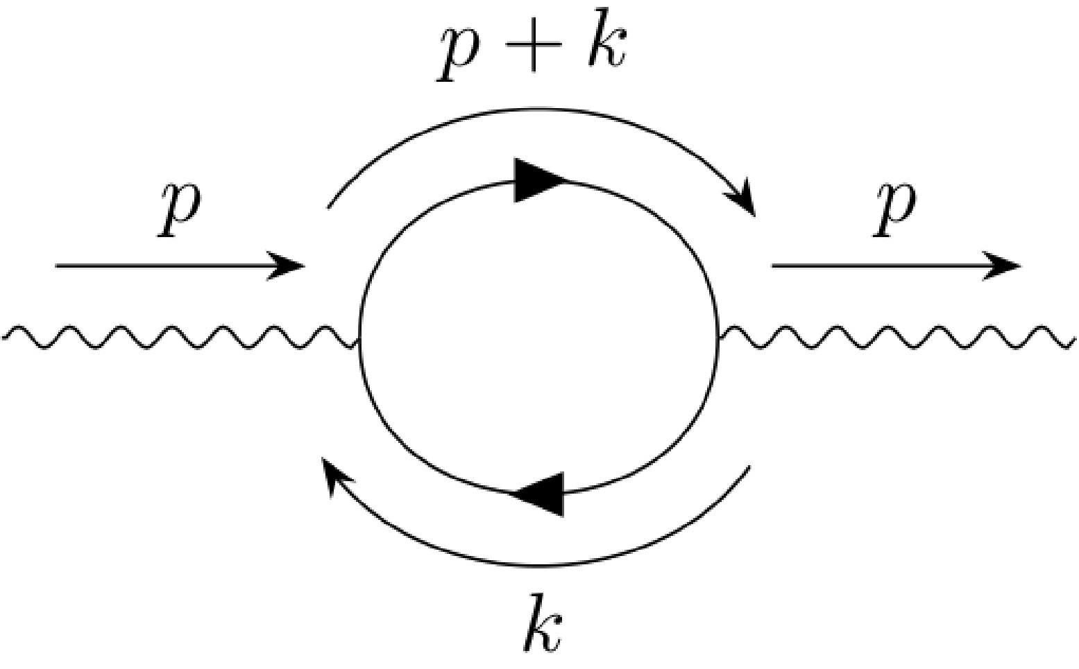

Figure 1.  Vacuum polarization diagram.

For a massless photon, one takes $ m_A^2 = 0 $, which holds in flat space. As we discuss further below and show in detail in [23], this is equivalent to the renormalization procedures used in [16, 18, 19]. However, as discussed above, a massless photon is inconsistent with a constant classical electric field in de Sitter space, which requires a tachyonic mass $ m_A^2 = -2H^2 $. Thus, we take the counterterm to be fixed by the condition

Note that, in contrast to the renormalization conditions defined (implicitly) in previous calculations in the literature, Eq. (11) is independent of considerations of the Schwinger current or renormalization. As we will see, with this renormalization condition, the renormalized Schwinger current in de Sitter space is not only UV finite but, crucially, is also free of the negative IR divergences found in previous calculations for both scalars [16] and fermions [19]. In [18], the authors argued that the negative IR-divergent current is not physical and correctly connected the origin of the issue with the renormalization condition, but they did not connect such a condition to the tachyonic mass of the vector in de Sitter space, which is a crucial point of our work.

When computing the vacuum polarization diagram, we cannot calculate the loop diagram analytically in de Sitter space. To obtain an analytic result, one must work in the Minkowski limit for both the spacetime integral and the electron propagator. The vacuum polarization diagram is then given by the well-known result from QED, which depends on the invariant mass squared $ (p^2) $ of the photon. This properly accounts for the UV modes in the counterterm, thereby allowing divergences in the regularized current to be canceled and ensuring a finite renormalized current. However, if we follow the renormalization procedure used implicitly in previous calculations [18] in the literature, assuming a massless photon and setting $ p^2=0 $, a negative IR divergence is introduced into the counterterm when the electron mass is taken to zero. As we show in detail in [23], this negative IR divergence is then introduced into the physical renormalized current, since there is no corresponding IR divergence in the regularized current, which is computed exactly, that could cancel it.

To see this explicitly, we take the standard flat-space result from scalar QED for the vacuum polarization [26]. Setting $ p^2 = 0 $, we have for the counterterm

with a factor of 4 included in the case of a charged fermion. Here, m is the mass of the electron, which enters through the propagator in the Minkowski limit, and Λ is the mass of the Pauli-Villars fields used to regulate the UV divergence (see Appendix A in [23] for details). With this counterterm, we can reproduce previous results in the literature for the renormalized current of a minimally coupled massive charged scalar [16, 18] and a massive charged fermion [19], which were obtained using different renormalization procedures. While the UV logarithmic divergence in Eq. (12) cancels the corresponding divergence in the regularized current, we explicitly see the negative IR divergence in the $ m \to 0 $ limit. However, as discussed above, the presence of a constant (dynamical) electric field in de Sitter space requires $ -p^2 = m_A^2 = -2H ^2 $, independently of renormalization or the Schwinger current.

For a charged scalar ϕ, if we instead evaluate the vacuum polarization diagram with $ p^2 = 2H^2 $, we obtain [23], in the limit $ m_\phi / H \to 0 $

which is seen to be IR finite. For a charged-fermion loop in the $ m_\psi/H \to 0 $ limit, we find [23]

which is again IR finite. Although Eq. (13) and Eq. (14) are obtained in the Minkowski and large-loop-momentum limits, they are perfectly self-consistent and free of IR divergences, which have been cured not by hand but by imposing the tachyonic photon mass condition needed to sustain a constant electric field in de Sitter space. This condition is independent of considerations of the Schwinger current or renormalization. As we discuss further below and show in detail in [23], these counterterms yield a renormalized Schwinger current that is both UV and IR finite.

Up to this point, our discussion has been completely independent of the Schwinger current. With the counterterm defined in Eq. (11), we can define the physical renormalized current. Varying the action in Eq. (8) with respect to the gauge field

Using the field configuration given in Eq. (3), we have $ \partial^\mu F_{\mu\nu} = -2 a H E \delta_\nu^z $. Although we treat $ A_\mu $ as classical, we compute a current arising from the quantum fluctuations of charged scalar and fermion fields. To compare such a current with the other classical terms in Eq. (15), we take its vacuum expectation value, $ \langle {{0}} | J_\mu | {{0}} \rangle \equiv \langle {{J_\mu}} \rangle $, where $ | {{0}} \rangle $ is the Bunch-Davies vacuum of the charged fields. This gives, for Eq. (15)

We have added the subscript 'reg' to the expectation value of the current, which is divergent and therefore must be regularized. We emphasize that the same scheme must be used to regularize both $ \langle {{J_\mu}} \rangle $ and $ \delta_3 $. With an appropriate renormalization condition to fix the finite part of $ \delta_3 $, we can obtain an unambiguous renormalized current

Calculating $ \langle J_z \rangle_{\rm{reg}} $ is involved, and we refer the reader to [16, 18, 19] for details. We have repeated the calculation [23] and confirmed previous results for both scalars and fermions. The result is non-perturbative, containing all effects from de Sitter space and, crucially, exhibiting no IR divergence in the small-electron-mass limit.

In contrast, the counterterms in Eq. (13) and Eq. (14) have been obtained by taking the Minkowski and large-loop-momentum limits in the vacuum polarization diagram. Thus, the only information they contain about de Sitter space enters through the tachyonic condition $ p^2 = 2H^2 $. Therefore, although there is no IR divergence, we should not expect them to properly capture all IR behavior. This can be seen in Eq. (13) and Eq. (14), which contain small, constant negative finite parts that, in the small-electron-mass limit, lead to a constant but slightly negative renormalized current [23]. This implies the unphysical behavior of a current flowing opposite to the electric field.

We expect that including corrections to the vacuum polarization from de Sitter space ensures a positive current, but in general, these corrections cannot be included analytically. One correction that can be included analytically is the curvature correction to the electron mass arising from a non-minimal coupling to gravity in the case of a scalar, or from the spin connection in the case of a charged fermion. These corrections are automatically included in the regularized current, which is computed non-perturbatively in de Sitter space directly from the Lagrangian.

In the calculation of the counterterm, the curvature corrections enter through the mass in the electron propagator. To see this, consider the equations of motion in a curved background for a free scalar ϕ with non-minimal coupling to gravity ξ and a free fermion ψ

The latter is obtained [27] by squaring the Dirac operator, $\;\not{ D} \;\not{ D} \psi =0$, with $\,\not{ D} = \gamma^\mu D_\mu$ and $ D_\mu = \partial_\mu + B_\mu $, where $ B_\mu $ is the spin connection. One consequence of the curved background is the addition of a term proportional to R in the Klein-Gordon equation. In particular, in de Sitter space, where $ R=12H^2 $ is constant, such a term can be incorporated into the squared mass term. Thus, we can take the free scalar propagator to be proportional to $ (k^2 + m_\phi^2 + \xi R)^{-1} $ and the free fermion propagator to be proportional to $ (k^2 + m_\psi^2 + R/4)^{-1} $. There are additional time-dependent corrections from de Sitter space in the □ operator that our calculation does not account for, but, to the best of our knowledge, they cannot be computed analytically. Nevertheless, we expect that, if the full calculation of the counterterm in de Sitter space were eventually performed, the resulting renormalized current would be positive in all regimes.

With these modified propagators, we repeat the calculation of $ \delta_3 $ in Minkowski space. Imposing the renormalization condition in Eq. (11), we obtain the finite parts of the counterterms (see Appendix A in [23] for details)

for the scalar case, whereas for the fermion case we obtain

where we have defined $ \overline{m}_\phi \equiv m_\phi/H $ and $ \overline{m}_\psi \equiv m_\psi/H $ and taken $ R = 12H^2 $ for the curvature in de Sitter space. We see explicitly that the curvature corrections to the electron mass give additional positive finite contributions to the counterterm. In the massless-electron limit, this leads to a positive finite part for $ \delta_3 $, in contrast to Eq. (13) and Eq. (14), where the curvature correction to the electron mass is neglected and the finite part is negative.

With these counterterms, we use Eq. (17) to obtain renormalized Schwinger currents for charged scalars and fermions that are UV- and IR-finite, as well as positive throughout parameter space. Explicit analytic expressions for the renormalized charged scalar and fermion currents are given in Eq. (22) and Eq. (23) of the Appendix, with details of the calculations provided in [23]. In Fig. 2, we show our results (solid) for the dimensionless Schwinger current $ {\cal{J}} \equiv \langle J_z \rangle_{\rm{ren}}/a e H^3 $ as a function of $ \lambda \equiv eE/H^2 $ for both scalars and fermions and for a few choices of parameters, as indicated in the figure. We see that the current is always positive for both fermions and scalars, with the scalar current multiplied by 2. For a minimally coupled scalar ($ \xi = 0 $), we see the IR hyperconductivity behavior found in [16, 18]. We also see that the current for a conformally coupled scalar ($ \xi = 1/6 $), which we have obtained here for the first time, has the same behavior as the fermion current. A detailed analysis of the behavior of the current in different limits can be found in [23].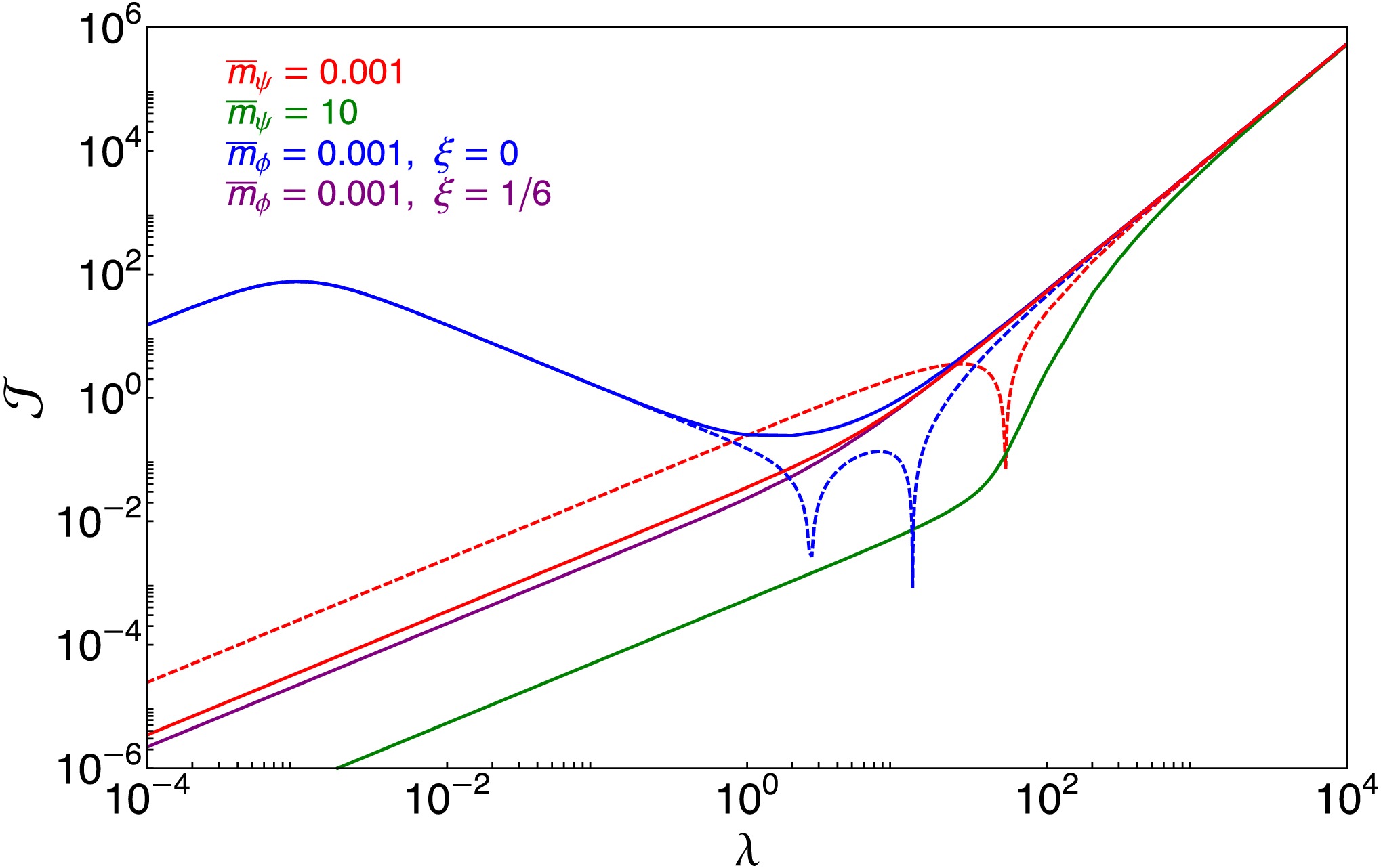

Figure 2.  (color online) The renormalized (dimensionless) Schwinger current $ {\cal{J}} \equiv \langle J_z \rangle_{\rm ren}/a e H^3 $ for a charged fermion (ψ) and scalar (ϕ, multiplied by 2) as functions of $ \lambda \equiv eE/H^2 $ (solid curves). Explicit analytic expressions are given in Eq. (22) and Eq. (23) of the Appendix. For comparison, we also show results for the renormalized Schwinger current obtained previously in the literature (dashed curves) [16, 19]. Between the cusps, the scalar current is negative, while the fermion current is negative to the left of the cusp; therefore, we have plotted the absolute value for each.

For comparison, we also show the currents obtained in previous results (dashed) in the literature [16, 19], which contain an IR-divergent $ \ln \left(m^2/H^2 \right) $ term arising from the implicit assumption of a massless photon in de Sitter space, as discussed above. Between the cusps, the scalar current is negative, while the fermion current is negative to the left of the cusp; therefore, we plot the absolute values.

We have revisited classical background electric fields and the Schwinger effect in de Sitter space, which can have important implications for the study of primordial magnetogenesis, inflationary dark matter production, and possibly other interesting cosmological mechanisms. We first pointed out that a constant electric field in de Sitter space requires the photon to have a tachyonic mass (see Eq. (6)). We then showed how this fixes the counterterm (see Eq. (11)) needed to absorb the single divergence present in the theory. With this counterterm, we recomputed the renormalized Schwinger currents in de Sitter space for both charged fermions and minimally coupled scalars, finding them to be UV and IR finite as well as positive for all parameter values. In particular, our results are free of the peculiar negative IR divergence found in previous calculations in the literature [16, 19]. We have traced the origin of this IR divergence to renormalization conditions that implicitly assumed a massless photon instead of a tachyonic one. We have also computed, for the first time, the Schwinger current in de Sitter space for a conformally coupled scalar, finding it to be positive and finite, with behavior very similar to that of the charged fermion current. Additional details and discussion of our analysis can be found in an accompanying paper [23].

We emphasize that, since the gauge field is not quantized (only the charged fields are), the one-loop calculation used to fix the counterterm contains the full quantum information, so our results are non-perturbative. The calculation of the regularized current is also non-perturbative and is performed in de Sitter space. However, since the counterterm is calculated in Minkowski spacetime, with the inclusion of curvature corrections to the electron mass and the imposition of the tachyonic photon mass condition, our final result for the renormalized Schwinger current is non-perturbative, but not exact. It can, in principle, be improved by calculating the counterterm with the full information of de Sitter space included. Nevertheless, our results resolve the puzzling IR behavior found in the previous literature and constitute an important step toward understanding the Schwinger current in de Sitter space.

The authors thank Pedro Garcia Osorio, Manel Masip, Jose Santiago, and Takeshi Kobayashi for useful comments and discussions.

Here, we give explicit expressions for the renormalized physical Schwinger currents for both non-minimally coupled charged scalars (ϕ) and fermions (ψ). Details of the calculation and analysis can be found in [23], to which we refer the reader. Defining the dimensionless ratios $ \lambda \equiv eE/H^2 $ and $ \overline{m}_\phi \equiv m_\phi/H $, we find the following expression for the renormalized charged scalar Schwinger current:

where we have defined $ \mu^2=\dfrac{9}{4} - ( \overline{m}_\phi^2 + 12\xi) - \lambda^2 $, and ξ denotes the non-minimal coupling to gravity. Defining the dimensionless ratio $ \overline{m}_\psi \equiv m_\psi/H $, we find the following expression for the renormalized Schwinger current of charged fermions:

where we have defined $ x \equiv \sqrt{ \overline{m}_\psi^2+\lambda^2} $.