Quasinormal modes of an electrically charged Kalb-Ramond black hole

A candidate for Planck-scale signals emerging from the underlying unified quantum gravity theory is Lorentz violation (LV). Among theories incorporating LV, explicit LV is a significant category. Its defining characteristic is the presence of vacuum expectation values (VEVs) that remain invariant under active (or particle) Lorentz transformations. A geometrical framework allowing for nonzero vacuum quantities, i.e., the VEVs, that violate local Lorentz invariance but preserve general coordinate invariance is therefore required. Riemann-Cartan geometry is particularly well-suited for this purpose [1]. The Standard-Model Extension (SME) serves as a phenomenological effective field theory that describes explicit LV [2]. Notably, an interesting property to mention is that LV in flat spacetime is closely connected with CPT violation [3, 4].

One attractive and generic mechanism of explicit LV is spontaneous LV [5]. It was first proposed in string theory and was considered to be a distinctive feature of string theory—unlikely to occur in four-dimensional renormalizable gauge theories. The basic idea is that a field with a negative mass-squared term possesses an unstable vacuum. In string field theory, tensor fields obtain such negative mass-squared terms through cubic interaction of the form $ ST^MT_M $ with the scalar field S having a negative VEV, such as the tachyon field. Here, the index M denotes one or more Lorentz indices. Another mechanism giving rise to explicit LV is noncommutative field theory, which is equivalent to a subset of the SME [6]. The commutator of spacetime coordinates is said to have the properties of the VEVs of fields in the string spectrum. Such a structure occurs naturally in string theory [7]. Furthermore, Ref. [8] demonstrates that birefringence effects are allowed in this theory.

It has also been suggested that certain theories such as loop quantum gravity [9] and multiuniverses [10] might generate birefringence effects [9, 11] that provide evidence for LV. However, the nature of LV in these frameworks differs intrinsically from the Lorentz gauge symmetry violation. Moreover, it is not caused by VEV-type coefficients for LV. Instead, LV in loop quantum gravity reflects the feature of the chosen semi-classical state rather than an inherent feature of the fundamental theory [9, 12], while LV in multiuniverses is more likely to be assuming a complete breakdown of Lorentz invariance [10, 13, 14]. Given that this paper focuses on the spontaneous violation case, our analysis should not be regarded as representative of all possible forms of LV.

A vector-induced model, now commonly referred to as the Bumblebee model, has drawn wide interest [2, 15]. A frequently used picture for understanding LV in this particular model emphasizes that the VEV of the vector field implies a preferred direction at each point in spacetime. It is also worth noting that the theory imposes constraints on the compactification of the extra dimensions [15]. However, the Bumblebee model is a minimal framework containing the feature of spontaneous LV. Instead, we focus on a tensor-induced model based on the Kalb-Ramond (KR) field, which has a well-defined origin in string theory.

The KR field, also known as B-field, was first proposed in the study of interstring interactions [16]. In modern textbooks, it is described as the antisymmetric 2-tensor that appears alongside the graviton and dilaton in the massless excited state in the oriented closed string spectrum (see e.g. [17]). In the context of superstring and heterotic string theories, it arises specifically as part of the NS-NS sector. The ten-dimensional Einstein-Kalb-Ramond action was first presented in Ref. [18]. In four dimensions, the KR field strength 3-form can be written with its dual 1-form T. One can show that $ {\bf{T}} = {\rm{d}}\chi $ is also exact if the first homology group of the spacetime manifold is trivial. The χ field has long been considered as an axion field despite its tendency toward dynamical instability. It was suggested by Ref. [19] that Routh's method can solve the problem caused by the noncommutativity between varying the action with respect to the metric field and substituting the KR field with the χ field. Later, it was shown that a candidate for the hypothetical axion field is the dual incarnation of the KR field in KK-compactifications of heterotic string theory to 4d [20, 21].

We note that a recent publication argued that nonbirefringence might serve as a key feature of quantum gravity because the extended action allowing nonbirefringence matches with the effective action of type II theories [22]. Previous research indicates that Bumblebee theory predicts birefringence while parity violation with the KR field forbids this effect [23]. However, although the effective Lagrangian given by the four-point scattering amplitude in type II string theory does possess the same form as the extended action analyzed, the latter is not the complete modification unless a field redefinition is performed to incorporate the other fields, including the KR field and the dilaton field [24, 25, 26]. Moreover, unlike spontaneous LV, the theory here is not derived from string field theory. Hence, these considerations shall not exclude the possibility of introducing a KR-induced LV Lagrangian.

Since black holes with axion hair have long been studied, a Lorentz invariant KR-induced axion-KR solution was soon suggested in Ref. [19]. A non-minimal coupling of the KR action inspired by superstring theory also appears to admit axion hair.

It was not until about 15 years ago that research began on a KR-field-induced spontaneous LV model [27]. Note that the “preferred direction” picture no longer applies in the model discussed here [2]. More recently, a static and spherically symmetric black hole solution was derived within this framework under the assumption of a non-dynamical KR field—implying that the field possesses only a specific VEV configuration [28]. Shortly thereafter, the same group proposed an electrically charged spherically symmetric KR black hole solution [29]. Reference [30] addresses the more general case of static, neutral, spherically symmetric black holes, and the authors subsequently extended this work to slowly rotating KR black holes later [31]. Various aspects of these black hole solutions such as the evaporation process have been extensively studied [32, 33, 34, 35]. Ref. [36] presents a new regular black hole solution within the framework of a non-commutative gauge theory applied to KR gravity.

In this work, rather than studying birefringence, we focus on the quasinormal modes (QNMs) of such a black hole solution obtained in a spontaneous Lorentz-violating scenario. While the QNMs of test scalar, Dirac, and vector fields in this spacetime have been previously investigated [33, 37], we consider gravitational and electromagnetic perturbations and the resulting coupled system. In gravitational-wave astronomy, it is the ringdown stage in the merger process of the binary systems that tells us the final state of their merger. This stage corresponds to the perturbation problem under certain spacetime considered—including the black hole background—the unique boundary condition of which at the horizon reflects the intrinsic dissipative feature of black holes. In particular, this constitutes an eigenvalue problem, the eigenstates of which are called QNMs. Although studies on QNMs started long before the first successful detection of gravitational waves, identifying the nature of the compact object was their main motivation at the very beginning [38, 39]. So the advent of gravitational-wave astronomy [40] has renewed interest in QNMs. The very first GW150914 data were already found to be consistent with the least-damped ringdown QNM [41]. Later, a convincing multimode black hole ringdown spectrum was observed using the gravitational wave event GW190521 [42]. Thanks to the loudness of GW250114, the latest progress has found not only a multimode spectrum but also higher overtones and has significantly improved the constraint accuracy [43].

The recent rise in interest in QNMs has also been driven by the discovery of their applications in the gauge-gravity duality, which was first proposed by Maldacena in string theory [44]. A correspondence between QNMs and the thermalization time scale in the dual conformal field theory (CFT) was first suggested and a qualitative agreement was found [45]. Subsequent work demonstrated a precise quantitative agreement between quasinormal frequencies (QNFs) and the poles of the retarded thermal correlation function, with exact expressions for the QNFs of various spins for the BTZ black hole [46]. A more general discussion was presented soon after [47]. General black branes have QNFs of a “hydrodynamic” form. This has led to a universal value $ 1/4\pi $ of the ratio of shear viscosity to entropy density of the dual QFT in the limit of gravity dual description [48, 49, 50]. This key result aids research into quark-gluon plasma (QGP) behavior and other topics.

Although QNFs can be analytically explained as the poles of the retarded Green's function, they must generally be solved numerically because the independent solutions of the perturbation equation can only be written analytically in a non-compact continued fraction form [51, 52]. Various numerical methods have been developed, among which the continued fraction method and the direct integral method are generalized to multi-field cases [53, 54]. The prevailing issue, however, is that in most cases when numerical precision is adequate, the frequencies of fundamental modes are identified merely by ranking their damping rate irrespective of the underlying physical state.

In this paper, we study the QNMs of an electrically charged spherically symmetric KR black hole proposed in Ref. [29]. We organize this paper as follows. In Sec. 2 we briefly review the electrically charged spherically symmetric black hole solution in a spontaneously Lorentz-violating theory induced by the VEV of the KR field. A minor error, which is insignificant at the background level, is identified to ensure the correct treatment of the problem at the perturbation level. Then, in Sec. 3, we study the perturbation problem of the solution. The odd-parity perturbation equations of both the gravitational field and the electromagnetic field are derived. We illustrate that these two equations cannot be decoupled. Our results and analysis will be shown in Sec. 4, where the numerical methods and our simple method are introduced. We apply and test this method for recognizing the different categories and use it to test our results and perform error analysis. The effects of LV on the QNMs are analyzed in the same section. Finally, we give a conclusion to our work in Sec. 5.

We briefly review the electrically charged spherically symmetric KR black hole proposed by K. Yang et al [29]. By introducing the KR field $ B_{\mu\nu} $ which has an appropriate VEV and a non-minimal coupling with gravity, the local Lorentz symmetry is spontaneously broken. The action can be written as

with $ H_{\mu\nu\rho}=\partial_{[\mu} B_{\nu\rho]} $ the KR field strength, $ \xi_2 $ and $ \xi_3 $ two coupling constants, and Λ the cosmological constant. The self-interacting potential $ V(x) $ is set to reach its minimum at $ x=0 $. The interaction between the KR field and the gravitational field follows Ref. [55], where the $ \xi_1 $ term considered in the general SME situation [27] has already been set to zero to obtain an analytic solution.

The KR field can be decomposed into pseudo-electric and pseudo-magnetic parts $ B_{\mu\nu}=\tilde{E}_{[\mu}v_{\nu]}+\epsilon_{\mu\nu\alpha\beta}v^{\alpha}\tilde{B}^{\beta} $, where v is a timelike 4-vector. It is assumed that the vacuum configuration of the KR field exhibits a pseudo-electric configuration $ b_{10}=-b_{01}=\tilde{E}(r) $, which thereby results in a vanishing KR field strength. Similar to the RN case, the background electromagnetic field in a spherical background can be set to an electrostatic form $ A_\mu=-\Phi(r)\delta_\mu{}^t $.

The Lagrangian of matter containing a non-minimal coupling between the electromagnetic field and the KR field is

where $ F_{\mu\nu}=\partial_{[\mu} A_{\nu]} $ is the electromagnetic field strength, and η is a coupling constant. The non-minimal coupling between the KR field and the electromagnetic field was proposed to support a consistent charged black hole. The three equations of motion can then be derived by varying the action with respect to the gravitational field, the electromagnetic field and the KR field as

where

One might wonder why there is no $ \xi_3 $ term in the equations. Some researchers have stated that this term can be absorbed by redefining the gravitational coupling constant in KR vacuum. It is worth mentioning that recent work [56] argued that this procedure leads to inequivalence under variation. Nevertheless, these equations can be viewed as being obtained by setting $ \xi_3=0 $ for simplicity, similar to the treatment of the $ \xi_1 $ term.

In the expression of $ T^M $ given in Ref. [28], the first term in the bracket appears to be inconsistent, likely due to an issue in handling the variation of the contraction with a symmetric tensor. This corresponding term in Ref. [28] is obviously asymmetric, whereas a symmetrized form, as presented in Eq. (4), is expected from a more detailed calculation. This discrepancy does not affect the background field equations, as both forms yield identical results under the specific configurations adopted for the background gravitational field, the KR field VEV, and the background electromagnetic field, since only two diagonal components, namely (0,0) and (1,1), contribute. However, the distinction may become relevant in the context of perturbations, where non-diagonal components are generally nonzero and could thus be sensitive to such differences.

Considering a static and spherically symmetric metric

under which we have $ \tilde{E}(r)=\pm\sqrt{\frac{b^2F(r)G(r)}{2}} $ (the sign does not matter since there are only quadratic terms of the KR field in the equations of motion), a solution was found in Ref. [28]. The equations of motion imply $ G(r)=F^{-1}(r) $. For the case of $ \Lambda=0 $, the result is [28]

where $ l\equiv\xi_2b^2/2 $ is the LV parameter. A similar solution has also been suggested within the framework of Bumblebee gravity [57]. Solving $ F(r)=0 $, we obtain the horizon radii:

which give a constraint on the parameters $ Q^{2}/M^{2}\leq(1-\ell)^{3} $ for a black hole solution. Note that this constraint also implies that $ \ell\leq1 $. In the following part of this paper, we will refer to this solution as a charged KR black hole.

We follow the general process proposed by Regge and Wheeler [58] to derive the perturbation equations. The perturbed metric and electromagnetic field can be written as follows:

where the quantities with a “bar” refer to the corresponding background field, and the perturbation fields are denoted by $ h_{\mu\nu} $ and $ a_\mu $. We first decompose the perturbations into scalar, vector and tensor parts according to SO(3) symmetry:

By using the spherical harmonic bases for SO(3) scalars

vectors

and tensors

we divide the perturbations into odd and even parity parts, where the lowercase Latin letter indices a, b, and c refer to θ and ϕ. The “odd/even parity” parts acquire a factor of $ (-)^{L+1} $/$ (-)^L $ under parity transformation. $ {\boldsymbol{\epsilon}} $ is the two-dimensional volume element (distinct from the total antisymmetric tensor density $ \epsilon $), and $ \gamma_{ab}=\bar{g}_{ab}/r^2 $ is the metric tensor on the sphere. We will only consider the $ M=0 $ cases due to spherical symmetry since the radial equations are independent of M after separating variables. In the following context, the index M will be omitted to prevent notational conflict with the black hole mass M.

Thanks to gauge invariance, the form of gravitational perturbations can be vastly simplified. Given a gauge transformation for odd and even gravitational perturbations respectively of the form $ \xi_{\mu;\nu}+\xi_{\nu;\mu} $, where the “coordinate transformation” covector $ \xi^\mu $ can always be written in the general form

we can always reduce the perturbation to a simple form

by solving the suitable coefficients $ \Lambda, \Theta_0, \Theta_1 $, and Θ.

The important thing here is that the gauge condition can be chosen for odd and even parity, respectively. Although the gravitational gauge transformations are usually considered as coordinate transformations, we are treating them here in perturbation theory as real gauge transformations without changing the coordinates [59]. Since we are not considering them as coordinate transformations, there is no need to worry about the perturbations of the electromagnetic field changing under these gauge transformations.

As mentioned before, this gauge-fixing procedure always works under a spherical background. One might check it and find that fixing the gauge is irrelevant to the specific choice of background metric as long as it has a spherical configuration.

As for the electromagnetic perturbation, it is just a covariant vector, so we directly write it in a simple form with our basic vectors

We focus on the odd-parity perturbation and follow the gauge choice in Ref. [60], such that the odd-parity perturbation does not change after gauge fixing.

Substituting the perturbed fields into Einstein's equations and Maxwell's equations and expanding them to linear order, we derive the perturbation equations. Owing to the spherical symmetry of the system, the odd and even parity parts of the equations can be decoupled, and the results are equivalent to those considering only odd or even parity perturbations. We will concentrate on the odd-parity parts. Due to the symmetry of indices in Einstein's equations, only four equations remain. Obviously, with merely three variables, only three equations are independent. Moreover, discovering that one equation acts as a constraint leaves precisely two equations. Transforming into the tortoise coordinate $ r_\ast $ defined as $ {\rm{d}} r_\ast=\frac{ {\rm{d}} r}{F(r)} $, and applying a variable substitution to the two remaining variables,

the equations can be further simplified

where the effective potentials are given by

These equations revert to those under an RN background when the LV parameter $ l\rightarrow0 $, which is consistent with our expectations.

It can be shown that these two odd-parity equations cannot be decoupled into purely gravitational and purely electromagnetic equations. We generally follow the decoupling process in Refs. [61, 62]. The basic idea is to make use of the diagonalization of matrices to eliminate the coupled terms in the equation set.

Equation (17) can be easily written in matrix equation form

where

Our primary objective is to decompose the effective potential matrix $ {\bf{V}}_{\rm{eff}} $ into the following form

where $ f_i(r) $ are some functions of r, and $ {\bf{C}}_i $ are radial-independent matrices that can be diagonalized by a radial-independent transformation matrix, $ {\bf{S}} $. For example, if there is just one term in the summation on the right-hand side of Eq. (21), then the effective potential can be diagonalized:

Since $ {\bf{S}} $ is independent of the radial coordinate, it commutes with the operator $ \left(\partial_{r_\ast}^2+\omega^2\right) $, as shown on the left-hand side of Eq. (22). In general situations, if and only if all the $ {\bf{C}}_i $'s can be diagonalized simultaneously, we can decouple Eq. (19)

In our case of the charged KR black hole

where

Simultaneous diagonalization is impossible since $ {\bf{C}}_2 $ and $ {\bf{C}}_4 $ are already diagonal but not identity matrices, while $ {\bf{C}}_3 $ is not diagonal. Therefore, these equations cannot be decoupled, and we need to apply numerical methods capable of finding the eigenvalues of a coupled equation set.

Due to the need to solve coupled differential equations, we choose the continued fraction method, also known as the Frobenius method, proposed by E. W. Leaver [52]. Here, we provide a brief overview of this method following [63]. Given an ordinary differential equation

in an asymptotically flat spacetime, a series solution can be written in the following form

where Ω, σ, and β are determined by boundary conditions, $ r_{+} $ is the event horizon, and $ r_{0} $ is an arbitrary parameter smaller than $ r_{+} $. This is the solution of Eq. (26) if and only if the series is convergent. Substituting the series solution into the equation, one can obtain an N-term recurrence relation for the coefficients $ b_i $

One might think that Eq. (28) is obtained from a power series, but since we need to change all the variables from r to $ x=\left(\dfrac{r-r_{+}}{r-r_{0}}\right) $, when we substitute $ R(r) $ into the equation, we have to multiply by a function of x to pick up terms of $ x^n $ and obtain the recurrence equations. This process can be thought of as a change of function bases. However, we will continue using the term “$ x^n $ term” for simplicity.

Usually, we shall decrease the number of terms in the recurrence relation to three using Gaussian eliminations

Equation (29b) directly shows

while Eq. (29a) gives a continued fraction form of $ b_1/b_0 $,

So the equation has a solution only if the right-hand sides of Eq. (30) and Eq. (31) are equal. If we set the boundary solutions on both sides as eigenstates for the same eigenvalue ω, this yields the eigenvalue equation, which can be numerically solved.

However, here we do not follow the usual procedure of finding the eigenvalue equation. Instead, we obtain the QNFs, i.e., the eigenvalues of the equation, by solving the secular equation of the set of recurrence relations [64]. This generalization to equation sets was first proposed in Ref. [53]. In the case of two coupled equations, Eq. (28) can be written as a matrix equation

where $ {\bf{C}}_{j,i}^{(N)}(\omega) $ are the two-by-two coefficient matrices of the ith recurrence equation, and $ {\bf{b}}_{i-j} $ are two-by-one vectors. Here, the phrase “the ith” represents the coefficient equation of $ x^i $, acquired by substituting the $ x^j $ term in the series solutions into the equation set and deriving the coefficients of $ x^i $. The four components of $ {\bf{C}}_{j,i}^{(N)}(\omega) $ correspond to the contributions of the two components of $ {\bf{b}}_{i-j} $ for the two equations, respectively. These recurrence equations can be organized into a block matrix form, similar to that referred to in Ref. [64], with a slight modification of notation for clarification. Theoretically, the order index i should extend to infinity, but in practical calculations, we must truncate the recurrence system at a finite maximum order $ i_{\max} $. The time required for calculation increases rapidly with an increase in the cutoff dimension. Unfortunately, unlike in the Schwarzschild and RN limits, the continued fraction method does not perform sufficiently well here under such low cutoff dimensions. Therefore, we will turn to the direct integration method.

The direct integration method is a straightforward approach to solving the equations of the QNM problem. The initial strategy involved calculating the Wronskian of the solutions integrated from both sides. However, this procedure was reported to suffer from numerical instability [65]. In Ref. [66], a variable substitution was introduced, which transforms the problem into solving a Riccati equation and looses the limitation of choosing the starting point of integration. A series expansion at both sides is then performed due to the approximation. The numerical method is then as described to vanish the difference of the two solutions (of a new variable ϕ) integrated from both sides. As shown in Ref. [66], the numerical instability is merely obscured rather than eliminated, so the method is only valid for frequencies with a smaller absolute value of their imaginary part compared to their real part.

A development of the method was made when searching for the QNMs of stars [67]. The authors directly integrated the Zerilli equation forward from the surface of the star to determine its asymptotic behavior in [66]. However, instead of merely vanishing the reflection coefficient, in that paper and many subsequent articles, they actually employed another method called the Breit-Wigner formula [68], which focuses on solving the real solutions for real frequencies and finding the real and imaginary parts of the eigenfrequencies by fitting the quadratic behavior of its flux near the minimum points. This alternative method is valid only under the Breit-Wigner assumption $ \omega_I\ll\omega_R $. Reference [69] proved the equivalence of these two methods, for the real parts of the frequencies, at least. The equivalence of finding the imaginary parts can only be verified numerically.

Both methods, which can be referred to as the direct integration method, have been generalized respectively to the cases of equation sets [54]. For a complete review, see Refs. [70, 71, 72]. Here we briefly outline the procedure.

For a free wave equation, the solution can be decoupled into a superposition of ingoing and outgoing plane waves. Therefore, at the boundary of our system, since the effective potentials tend to zero as $ r_*\rightarrow \pm\infty $, the asymptotic solution can be expanded into the formula

where $ {\bf{u}} $, $ {\bf{B}} $ and $ {\bf{C}} $ are vectors. At the same time, we need to cut the boundary at both ends, so the boundary condition is a little deviated from plane wave. We write the deviation as a series expansion to the nth order

Substituting this formula into the perturbation equations, a recurrence equation between the expansion coefficients can be obtained. Then all the coefficients can be written as combination of the zero-order coefficients $ {{\bf{b}}_{(h)}}_0 $

where we have dropped the subscribe “0” for simplicity. The matrix $ {\bf{M}}_{\rm{(h)}}(\omega,r) $ remains unchanged as long as the cutoff order n does not change. So $ {{\bf{b}}_{\rm{(h)}}} $ determines the boundary condition near the horizon completely. Choosing a set of orthonormal base of $ {{\bf{b}}_{\rm{(h)}}} $ as $ {{\bf{b}}^{(1,0)}_{\rm{(h)}}}=\left(\begin{array}{c} 1\\0 \end{array}\right) $ and $ {{\bf{b}}^{(0,1)}_{\rm{(h)}}}=\left(\begin{array}{c} 0\\1 \end{array}\right) $, any solution can be written as

Integrating $ {\bf{u}}_{\rm{(h)}} $ outward, we find the corresponding values of the solutions at infinity due to the linearity of integration

A similar expansion is to be made for solutions at infinity

The point is that we want to test whether the solution we just obtained through integration satisfies our boundary condition at infinity. Generally we have

from Eq. (38), where $ {{\bf{b}}_{\rm{(inf)}}}_0 \equiv {\bf{B}} $ and $ {{\bf{c}}_{\rm{(inf)}}}_0 \equiv {\bf{C}} $. We can express the zero-order coefficients inversely in terms of $ {\bf{Y}} $ and get $ {\bf{B}}^{(1,0)} $, $ {\bf{B}}^{(0,1)} $, $ {\bf{C}}^{(1,0)} $, and $ {\bf{C}}^{(0,1)} $, respectively. Since all the relations are linear, it is easy to prove that

where $ {\bf{A}} $ refers to $ {\bf{B}} $ or $ {\bf{C}} $. Finally, we arrive at the conclusion that ω is a QNF only if

We develop a method to recognize the eigenvalues of coupled equations that cannot be decoupled and to estimate the degree of coupling.

Strictly speaking, the eigenvalues and eigensolutions of a set of coupled equations that cannot be decoupled can only be explained as common eigenvalues and eigensolutions of the equation set. The eigenvectors do not follow a specific law. Conversely, for those that can be decoupled, e.g., in the RN case, under the decoupled form, it is easy to distinguish the difference between the gravity-eigenfrequencies and the electromagnetic-eigenfrequencies, since most of the eigenstate vectors are just the base vectors. Of course, the set of eigenfrequencies in the coupled form is the union set of those in the two decoupled equations, which means it may contain degenerate modes. However, the probability should be fairly low, which means we barely need to take account of them, especially when searching for fundamental modes.

If the equations are still coupled, the eigenvector would be transformed by a transformation matrix, just as shown in subsection 3.2. This might prevent us from recognizing whether the equations can be decoupled by just looking at the eigenstates. Examining the fraction of two components of the different eigenvectors under the same coefficients may solve the problem. But the real question is: is it really important to decouple the equations?

We have provided our proof of why our perturbation equations cannot be decoupled in 3.2. Some may doubt the non-decouplability, but the frequencies are indeed the right result since our numerical methods are reliable. It is just the explanation being different, as mentioned above, so the problem of decoupling really does not matter.

Despite all the above, for the specific problem we are dealing with, the modification caused by LV should be sufficiently small. So even if the equations cannot be decoupled, the degree of non-decouplability should be rather weak. Note that our perturbation equations degenerate to the coupled ones in the RN case. Thus, it is reasonable to infer that the eigenstates and eigenfrequencies obey a rule with just a small deviation from the RN case. So, we can still distinguish the spectrum slightly deviated from the RN gravity or electromagnetic spectrum by its eigenvectors $ {\bf{C}} $, or $ (a,b) $. Obviously, $ (a,b) $ should be equal to $ {\bf{C}}^{(a,b)} $ up to a scalar factor, at least for decouplable equation sets, considering the decoupled forms. The numerical results under the RN limit support this, which has also tested the effectiveness of our method. For instance, for the fundamental electromagnetic mode when $ l=0.01 $, $ \dfrac{C_1'}{C_2'}=4.74314-27.9028i $, while $ \dfrac{a}{b}=5.29009- 27.9246i $. We have proven that the linear combination coefficients of $ {\bf{C}}^{(a,b)} $ are the same as those of $ {\bf{B}}^{(a,b)} $. The only job left is to solve the equation

The problem is that the coefficient determinant of our equation merely approaches zero numerically, rather than strictly tending to zero. To find the numerical solution, take either of the two simultaneous equations and solve for the relation between a and b.

Remember that in the undecoupled form, the eigenstates are transformed by a matrix, so the ratio would not be $ 1/0=\infty $ or $ 0/1=0 $. They are completely dependent on the matrix, meaning we cannot distinguish the discriminant by just looking at the ratio itself. What we can determine is whether the ratio clearly separates into two categories, and we can distinguish them by other less indirect clues as shown in the following context. Since the eigenvector and transformation matrix are complex, based on both analytical and numerical considerations, it is reasonable that the ratio of the norm of the two components of the eigenvalues would be adequate for recognition, as long as this quantity clearly separate into two categories, as stated before. Consider the example of the eigenstate $ (1,0) $:

We emphasize again that all the results in this section are obtained from the odd-parity sector of the perturbation equations. As shown in 4.1, we use the Frobenius method to solve for the eigenvalues. The series solution is expressed as follows:

The fundamental QNFs for $ L=2 $ with different values of Q in the RN limit, i.e., $ l=0 $ are shown in Tables 1 and 2. By cutting off the dimension of the coefficient matrix at 40, we find that the fundamental QNFs of the charged KR black hole in the Schwarzschild limit coincide perfectly with those of the Schwarzschild black hole. The fundamental QNFs of the charged KR black hole in the RN limit have been calculated to test the validity of our code as well. We do not use the same cutoff dimension for different values of Q due to the limitation of computing time. However, we have noticed that the greater the cutoff dimension is, the closer the frequencies are to the values in the RN case. Therefore, the results are definitely reliable.

As already discussed, due to the numerical accuracy limitations of the continued fraction method ¹, we turn to the direct integration method to study the effect of LV on QNMs.

First, we test our discriminating method with eight different modes in the RN case with $ Q=0.1M $ and $ M=1 $, as shown in Table 3. The third columns, represented by $ |C^{(a,b)}_1|/|C^{(a,b)}_2| $, illustrates the feature of the eigenstates, as mentioned in Sec. 4.1.3. The ratio of the norm of the two components of the eigenvalues clearly separates into two categories. The differences within each column are caused by numerical errors of the state, since the odd-parity perturbation equations in the RN case can be decoupled. It is worth mentioning that the ratio depends on the parameters. The reasons for the influence on the ratio caused by Q and l are different. Q represents different decouplable RN cases, which means different transformation matrices, while l represents only a small deviation from the RN cases.

Table 4 shows the fundamental odd-parity QNFs of a charged KR black hole for different values of the LV parameter l. Our calculations are performed with $ Q=0.1M $ and $ M=1 $. Here, we provide the trial solution ² iteratively. The frequency results are not entirely accurate, which is due to the selection of parameters, as we will see shortly during the error analysis. However, these results assist in confirming our classification of modes. The separation of our discriminant remain intact, and its deviation from the RN case increases with a growing violation parameter l, although the deviation is relatively small. All the results support our analysis of identifying eigenvalues by examining the eigenstates. Every subsequent dataset will be tested by their discriminants.

We mentioned above that the data in Table 4 are somewhat unreliable, which is implied at first glance by its discontinuity with the fundamental QNFs in the RN case. We also encountered further specific issues. All these issues stem from three influential factors. First, the values of the violation parameter l are too large. As will soon be presented, within the current numerical implementation, larger values of l appear to make the calculation more sensitive to the boundary cutoff, expansion order, or trial solution. Worse still, excessively large values of l will even cause the disappearance of a steady solution with respect to the position of the boundary. Physically, the violation of Lorentz symmetry cannot be apparent because of the broad support of general relativity from various tests, which means l must be extremely small. In a bumblebee-induced model, l has already been limited to the level of $ 10^{-13} $ [73]. The problem of discontinuity can be avoided by choosing sufficiently small values of l. The second factor lies in the expansion order at the boundary. The final factor is the position of the boundary. When taking different values of $ r_{\rm{inf}} $, we obtain different results. For example, we take the trial frequency $ \omega_{\rm{trial}}M=0.388399-0.0731774i $ given by the continued fraction method, which belongs to the gravitational category in the RN case, the results are

We can see that the first result still belongs to the gravitational category, while the second one belongs to the electromagnetic category. Because the wave function will diverge at infinity, $ r_{\rm{inf}} $ should be chosen with a proper value rather than a larger one.

From now on, we take the same trial solution $ \omega_{\rm{trial}}M=0.373294-0.08866{\rm{i}} $, which is the fundamental odd-parity gravitational QNF of the RN black hole with $ Q/M=0.1 $. Figure 1 shows the results of our error analysis. This is a scatter plot, and we connect the data points with lines for convenience. Different spiral lines represent different violation parameters, while each point on a line corresponds to a different $ r_{\rm{inf}} $ value, which increases in the direction of the arrows. The blue line represents the RN case, and $ r_{\rm{inf}} $ increases anticlockwise, similarly to the other spiral lines. The cutoff ranges from 16 to 35 on the blue line, on which the red point represents $ r_{\rm{inf}}=25 $. On the other lines, $ r_{\rm{inf}} $ ends at 25 where the arrows are placed. The green line is obtained by changing l while fixing $ r_{\rm{inf}}=18 $, the effect of which is to be explained later. We do not take the trial solution in an iterative way as in Table 4 because the values of l we take are adequately small in general.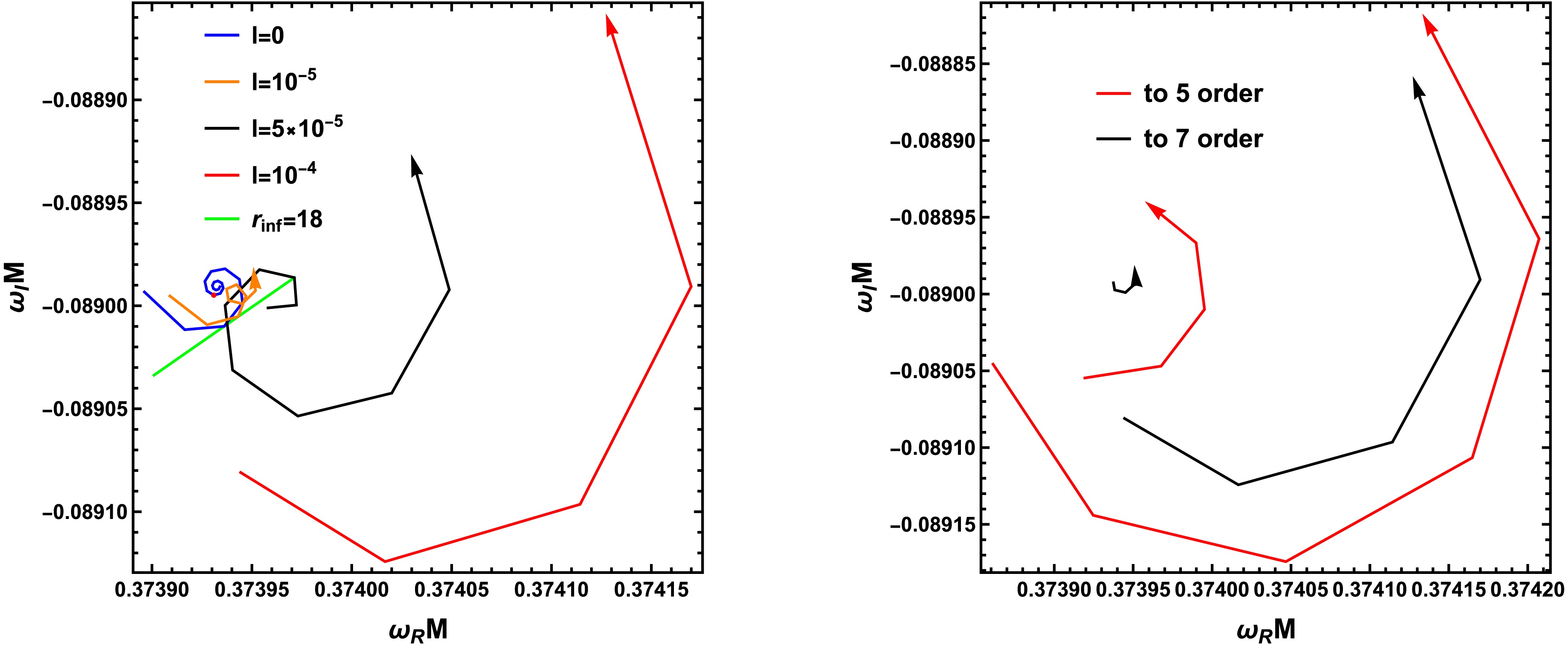

Figure 1.  (color online) Error analysis.

As can be easily read from the figure, all the results follow a similar spiral behavior. With a relatively appropriate choice of l, there exists an “innermost circle” which implies that in some region of $ r_{\rm{inf}} $, we can get a steady solution. Away from the “innermost circle”, the scale of spiral lines increases with l, while the “phase” of which does not change. The result is that even when fixing an inappropriate value of cutoff $ r_{\rm{inf}} $, one would always get a linear behavior between ω and l, which seems to be a good result for some careless people. But actually, it is not, and when choosing even neighboring $ r_{\rm{inf}} $'s, one would find very different trends. This is more intuitive in Fig. 2; the trend can even change from increasing to decreasing with l. Surely, this analysis only stands when the parameters chosen are approximately appropriate; otherwise, one would find solutions in the wrong category. Note that all points here being recognized as belonging to the expected category can be viewed as another criterion that our results are reliable. Meanwhile, the “innermost circle” may not even exist for an excessively large l, which explains the emergence and disappearance of the discontinuity problem mentioned above. After all these analyses, it is obvious that we should focus on the “innermost circle” of each fixed l. Note also that the accuracy of a single point is actually adequately well; it is just not enough when studying the effect of l.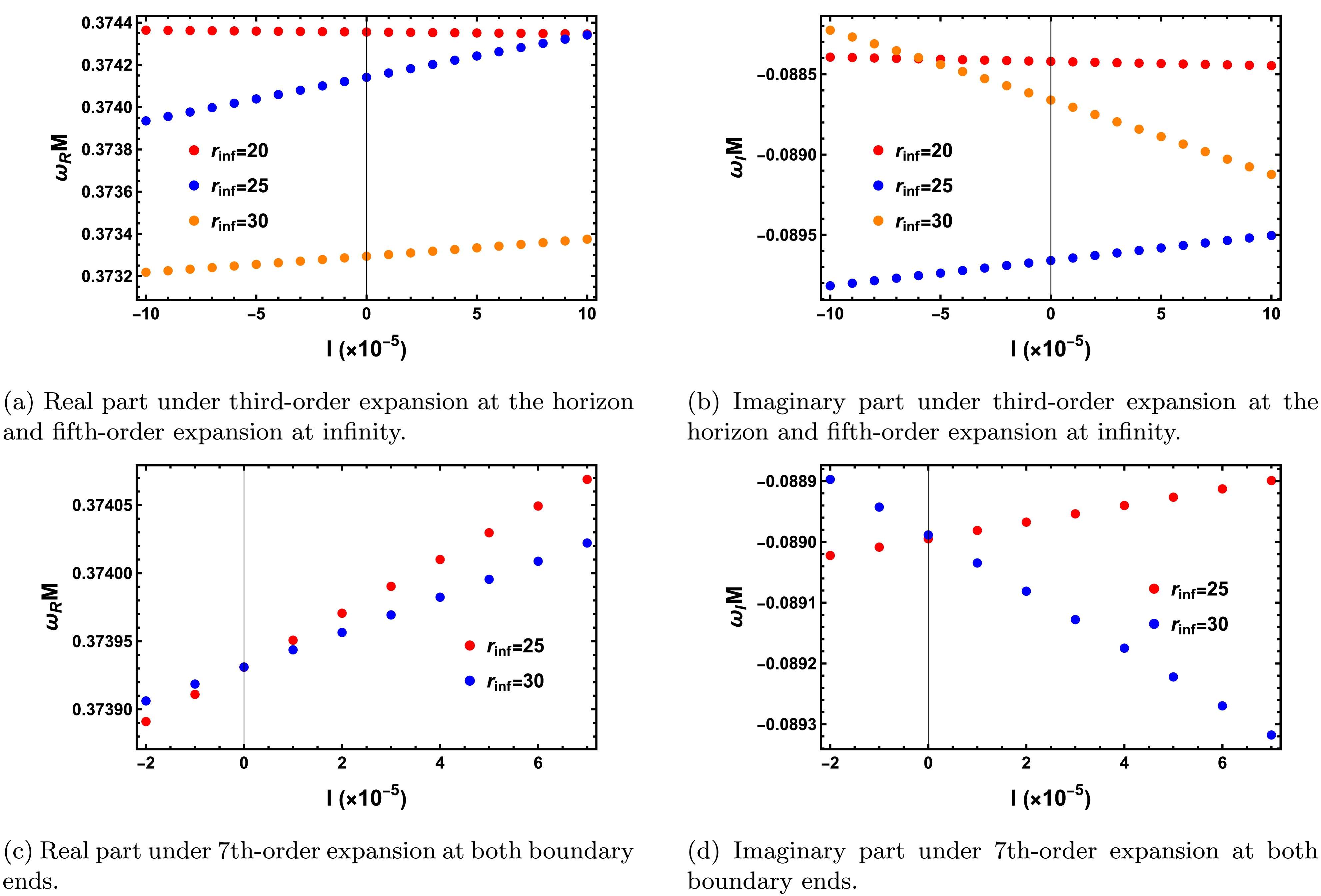

Figure 2.  (color online) The trend of gravitational fundamental QNF with respect to the violation parameter l under different boundary cutoff $ r_{\rm{inf}} $.

We have to mention that the same problem does not exist in the RN case. Figure 3 shows that the spiral lines obtained under different Q's are of the same scale and “phase”. As a result, for any fixed cutoff of appropriate magnitude, results do reflect both real and imaginary part behaviors.

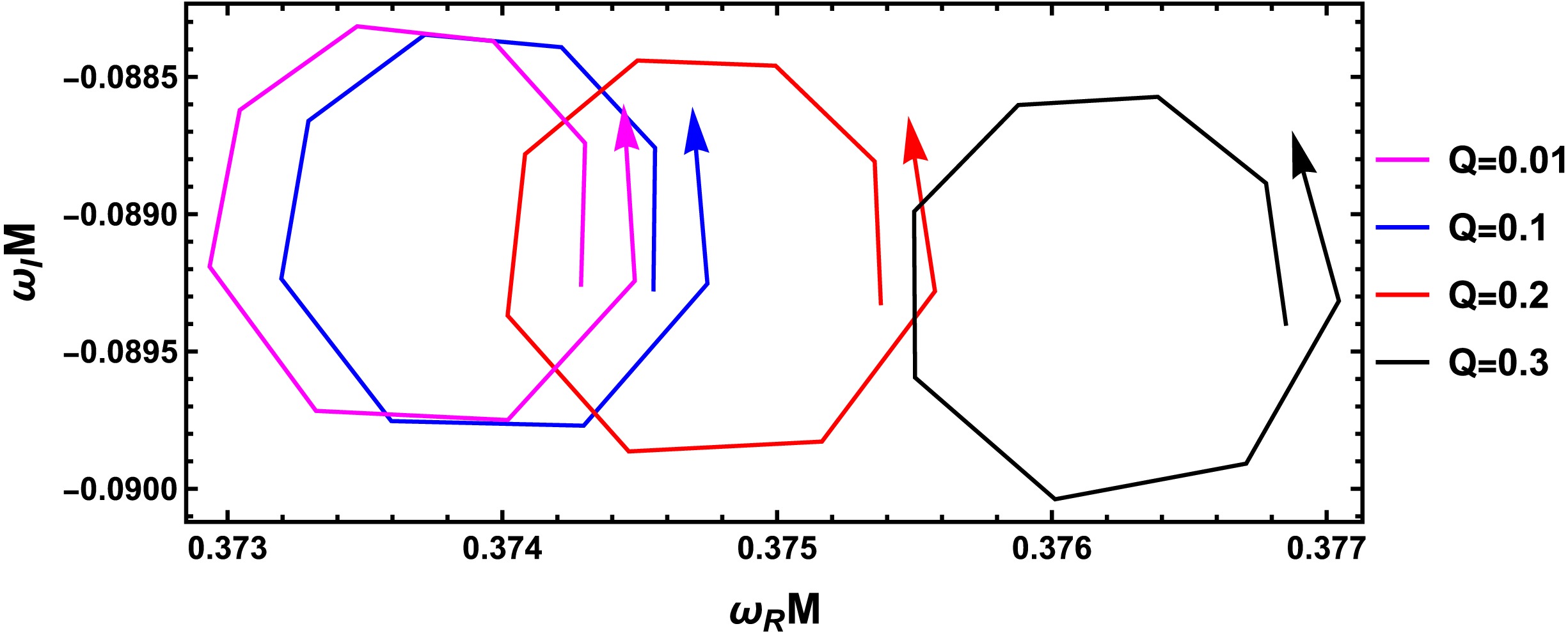
Figure 3.  (color online) Error analysis in RN cases under third-order expansion at the horizon and fifth-order expansion at infinity.

Another thing to mention, from the analyses above, the impact of cutoff $ r_{\rm{inf}} $ on the results is very significant. We have to emphasize that the influence of cutoff is caused by wavefunction-divergence-induced numerical overflow instead of the deviation of effective potentials shown in Figs. 4 and 5. From the graphs, it is easy to see that the influence on effective potential by violation parameter l is very small relatively.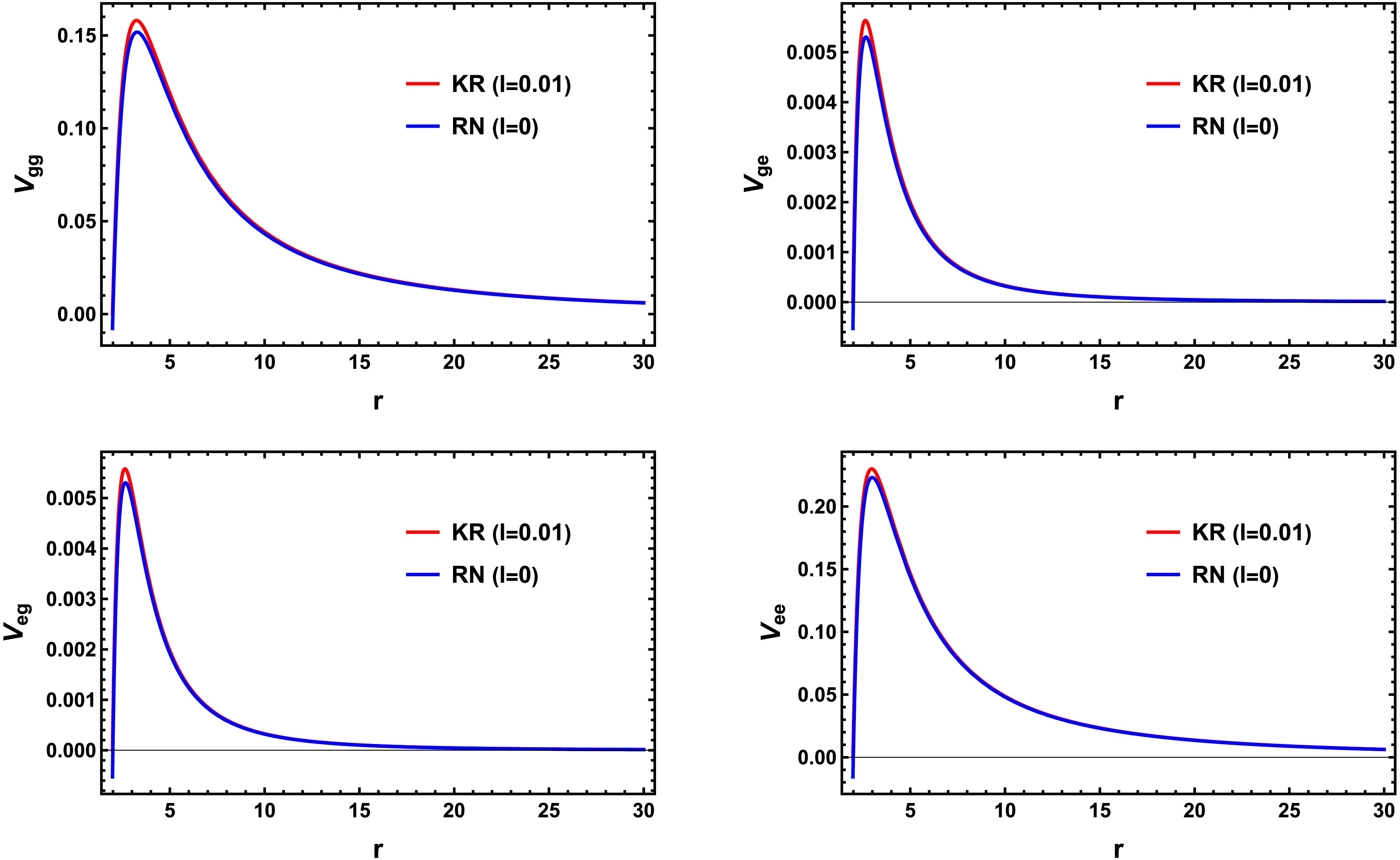

Figure 4.  (color online) Effective potential components compared with the RN case.

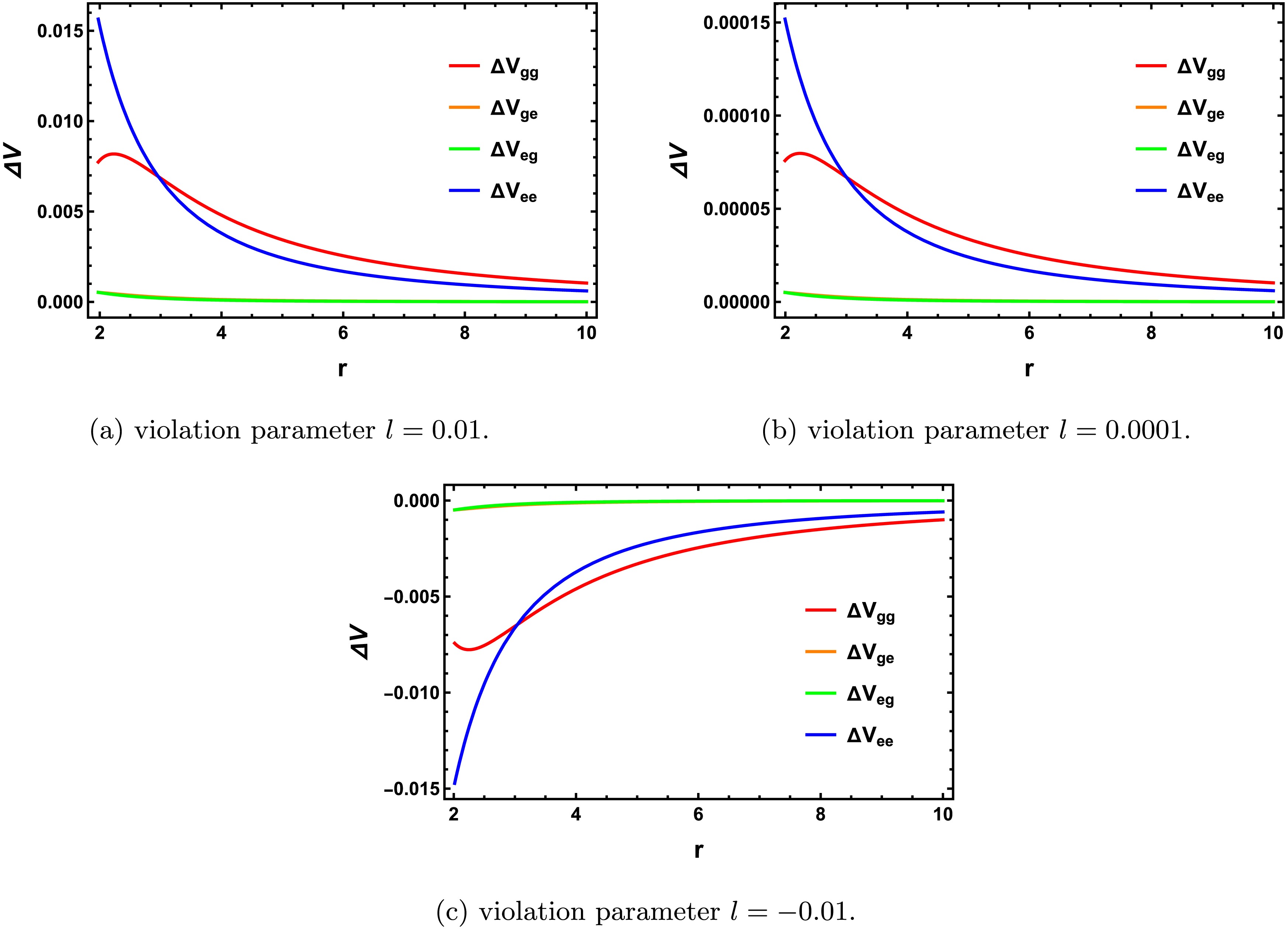
Figure 5.  (color online) Deviation of effective potential components from the RN case at different violation parameter l.

We then study the movement of the “innermost circle”. Figure 1b shows the improvement brought by increasing the order of expansion at the boundary, but the calculating time increases rapidly. Since we aim to investigate how the “innermost circle” behaves with respect to the violation parameter, it is beneficial to choose as high an order of expansion as possible. Alternatively, at the very least, the analysis should be conducted over a wider range of l. This is because using a lower order of expansion might cause multiple “innermost circle”s to nest within the same region of l. We finally choose an order of expansion of 7, controlling the calculating time of one point to about one day on a personal computer. Again, in Fig. 1a, the key difference among the spiral lines is the region near the “innermost circle”s. The corresponding $ r_{\rm{inf}} $ of the “innermost circle” for different spiral lines decreases with increasing l. So theoretically there is no appropriate choice of a fixed $ r_{\rm{inf}} $. For each l, the “innermost circle” has to be found, but this would require too much time. Observing the left three spiral lines in Fig. 1a, the “innermost circle”s almost move horizontally to the right. This means that the real parts of the fundamental odd-parity mode increase obviously with l, while the imaginary parts stay unchanged, or at least insufficient to be studied under the current level of accuracy. Now we focus on the green line, $ r_{\rm{inf}}=18 $ is on the “innermost circle”s of some spiral lines when l is relatively larger as on the black one, but for other spiral lines, for example, the orange and blue ones, the real parts of the points on the green line are almost the same as the real parts of the corresponding “innermost circle”s. So we calculate the trend of real parts of gravitational fundamental odd-parity frequencies with the green line as shown in Fig. 6. This is a little opportunistic but reasonable way we apply. Of course, we view the imaginary parts as not changing, and can be set directly as the frequency in the RN case. It shows that the real parts increase linearly with l at least within a proper region of l.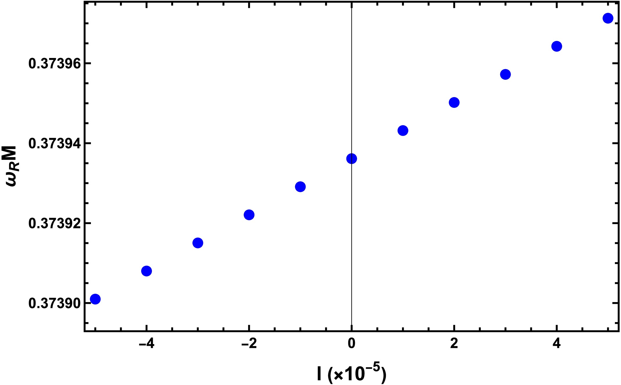

Figure 6.  (color online) Effect of violation parameter l on the real part of gravitational fundamental QNF with boundary cutoff $ r_{\rm{inf}}=18 $ under a 7th-order expansion at both boundary ends.

As mentioned above, the LV parameter l in the bumblebee-induced model has been constrained to the order of $ 10^{-13} $ [73]. Under this constraint, the resulting QNM spectrum would likely remain very close to the RN limit. Since the violations in both the Bumblebee- and KR-induced models are caused by spontaneous LV, the restriction can definitely be referred to here in our case. Because continuing lowering l may increase the calculating time significantly, our choice of l is not sufficiently small. But we can reasonably infer from the linear behavior we obtained of the real part and the invariance of the imaginary part of the fundamental odd-parity gravitational frequencies when l is set to less than $ 10^{-13} $.

LV is a possible Planck-scale signal of modified gravity. A natural way of generating it in string theory is through spontaneous LV. The KR field, dual to the axion field, can induce this process.

In this paper, the perturbation problem of an electrically charged spherically symmetric KR black hole was studied. The focus is mainly on the odd-parity sector. A method was developed to identify the eigenvalues, especially for nearly decouplable equation sets. We performed a numerical error analysis of the matrix-valued direct integration method. The results help us choose the appropriate range of the violation parameter and the boundary cutoff. Our calculation shows that the violation parameter mainly causes a linear deviation of the real parts of the fundamental odd-parity modes with l, while the imaginary parts remain unchanged. We also presented the remaining problems at the very end.

It is worth mentioning that, since our research was based on a black hole spacetime purely caused by spontaneous LV, there is a strong probability that the behavior of QNFs presented here cannot be generalized to phenomenological research including more general Lorentz-violating cases as mentioned in the introduction. Therefore, studies are underway to recognize different kinds of LV, or perhaps a more general description of LV beyond SME is expected to be conducted.