Amplitude analysis of charmed-meson decays at BESIII

The necessity of amplitude analysis stems from the inherent disparity between the experimental capabilities and theoretical formulations in particle physics. Experimentally, typical detectors directly observe only stable or sufficiently long-lived particles such as $ e^\pm $, $ \mu^\pm $, $ \pi^\pm $, $ K^\pm $, p, and γ. Other common final states such as $ K_S^0 $ and $ \pi^0/\eta $ are reconstructed via their decays $ K_S^0 \to \pi\pi $ and $ \pi^0/\eta \to \gamma\gamma $, respectively. These constitute the experimentally accessible final-state particles. Conversely, short-lived resonances such as $ K^* $, ϕ, and $ a_0/f_0 $ [1, 2] decay promptly and evade direct detection. However, theoretical frameworks are largely agnostic to the stability of the decay products. Owing to the nonperturbative nature of the strong interaction, rigorous theoretical predictions for multibody decays remain highly challenging and are often constrained to two-body or quasi-two-body intermediate processes.

Decay modes yielding three or more final-state particles inherently exhibit quantum interference among intermediate resonant states. For example, the final state of $ D^0 \to K^- \pi^+ \pi^0 $ receives interfering contributions from intermediate processes such as $ D^0 \to \bar{K}^{*0} \pi^0 \to K^- \pi^+ \pi^0 $ and $ D^0 \to K^{*-} \pi^+ \to K^- \pi^+ \pi^0 $ [1]. Although experiments measure the kinematic phase space (four-momenta) of the final-state $ K^- $, $ \pi^+ $, and $ \pi^0 $, the theoretical calculations are tractable for the quasi-two-body transitions $ D^0 \to \bar{K}^{*0} \pi^0 $ and $ D^0 \to K^{*-} \pi^+ $. Therefore, extracting the underlying intermediate dynamics from final-state kinematics while rigorously accounting for quantum interference is crucial to test theoretical models. Amplitude analysis provides the essential mathematical framework to bridge this experimental-theoretical divide.

The Beijing spectrometer III (BESIII) experiment located at the Beijing electron positron collider II, operates as a dedicated τ-charm factory. Over the past decade, BESIII has accumulated an unprecedentedly large data sample of $ e^+e^- $ collisions at a center-of-mass energy of $ \sqrt{s}=3.773 $ GeV, reaching an integrated luminosity of $ 20.3\; \text{fb}^{-1} $ [3]. In addition, the experiment has collected about $ 7.33\; \text{fb}^{-1} $ of data in the center-of-mass energy range between 4.128 and 4.226 GeV. The threshold production of $ D\bar{D} $ and $ D_s^*\bar{D_s} $ pairs provides a uniquely clean experimental environment. $ D_{(s)} $ and $ \bar{D}_{(s)} $ mesons are produced nearly at rest, with only the $ D_{(s)}\bar{D}_{(s)} $ pair and no additional hadrons, thereby leading to low background and high detection efficiency. These features make BESIII an ideal laboratory for studying D meson decays.

The remainder of this paper is organized as follows. Section II details the construction of the probability density function and the likelihood function employed in the amplitude analyses, Monte Carlo (MC) integration techniques, treatment of detection efficiency and experimental resolution, and background modeling. Section III outlines the amplitude formalism governing the decay dynamics of D mesons implemented in BESIII measurements. Finally, Section IV provides a summary and explores the advanced applications of these methodologies.

In the amplitude analysis of a multibody decay involving three or more final-state particles, the relative magnitudes and phases of the intermediate decay processes are extracted via fits to the data samples. Other properties such as resonance masses and widths may also be treated as free parameters if required. This section details the construction of the likelihood and probability density functions (PDFs) based on the amplitude models for unbinned maximum-likelihood fits.

The signal PDF, which represents the probability density of a specific kinematic configuration p, is defined as

where $ \epsilon(p) $, $ R(p) $, and p represent the detection efficiency, phase-space (PHSP) factor, and set of kinematic variables characterizing a decay event, respectively. The total amplitude $ {\cal{M}}(p) $ is the coherent sum of amplitudes that corresponds to intermediate processes given by

where $c_n = \rho_n {\rm e}^{{\rm i}\phi_n}$ and $ {\cal{A}}_n $ represent the complex coefficient and dynamic amplitude for the $ n^{\mathrm{th}} $ intermediate process, respectively. The magnitude $ \rho_n $ and phase $ \phi_n $ are free parameters in the fit. The formalism of individual amplitudes is detailed in Section III.

Although amplitude $ {\cal{M}}(p) $ isolates the pure decay dynamics of a D meson independent of detector effects, experimental data are inevitably subject to a nonuniform detection efficiency. To construct a PDF that models the measured event distribution accurately, the efficiency $ \epsilon(p) $ must be incorporated as a multiplicative factor. The set of kinematic variables p typically comprises the four-momenta of the final-state particles. For the decay of a spin-0 mother particle (e.g., a D meson) into $ N\geq 3 $ particles, the number of degrees of freedom is $ 3N-7 $. This is derived from the $ 3N $ momentum components, subtracting four constraints from energy-momentum conservation and three Euler angles that define the overall spatial orientation of the final-state system. Owing to the isotropic nature of the decay in the rest frame, these three angles can be ignored. Further details are available in Chapter 49 of the Particle Data Group review [1]. The PHSP factor $ R(p) $ encodes the kinematic phase-space density; its functional form depends on the specific choice of coordinates. This factor remains constant over the allowed PHSP boundary when parameterized directly in terms of the four-momenta; however, it may vary in other coordinate representations. Its analytical form derives from the Jacobian determinant associated with the coordinate transformation. Furthermore, the integral in the denominator ensures that the signal PDF is strictly normalized to unity over the entire PHSP, fulfilling the fundamental mathematical requirement of a PDF.

The likelihood for a given dataset is constructed as the product of the PDF evaluated at each measured event.

where k runs over all events in the data sample, and $ N_{\mathrm{data}} $ represents the total number of events. Consequently, the log-likelihood function, which is maximized during the fitting procedure, is given by

The term $ \sum \ln[\epsilon(p_k) R(p_k)] $ is independent of the fit parameters, and therefore, it acts as a constant offset and can be omitted during the maximization process. Parameter estimation is driven entirely by the first term. Moreover, the normalization integral in the denominator can be approximated efficiently via MC integration, which is a technique detailed in Section II.A. This reveals an elegant feature of the amplitude-analysis formalism: parameter extraction can be performed without requiring a priori analytical knowledge of the explicit efficiency and PHSP functions.

In the presence of non-negligible background contributions, the likelihood is extended by incorporating a normalized background shape $ {\cal{B}}(p) $.

where $ w_{\mathrm{sig}} $ represents the signal purity of the data sample. By defining an efficiency- and PHSP-corrected background PDF as $ {\cal{B}}_{\epsilon}(p) = {\cal{B}}(p)/[\epsilon(p) R(p)] $, the term $ \epsilon(p_k) R(p_k) $ can be factored out. Then, the modified log-likelihood becomes

As indicated previously, the additive $ \ln[\epsilon R] $ term is dropped during the fit. The corrected background shape $ {\cal{B}}_{\epsilon}(p) $ is obtained through multidimensional reweighting techniques (discussed in Section II.B) utilizing the background distribution $ {\cal{B}}(p) $ modeled from inclusive MC samples or data-driven sideband estimations.

An alternative strategy to handle backgrounds is to subtract their contribution directly from the log-likelihood function using simulated or control events.

where l iterates over events in a dedicated background sample, $ N_{\mathrm{bkg}} $ represents the total number of such background events, and the statistical scaling weight $ w = (1-w_{\mathrm{sig}}) N_{\mathrm{data}}/N_{\mathrm{bkg}} $ ensures proper normalization based on signal purity. The prefactor ensures the correct estimation of statistical uncertainties. However, this background-subtraction approach can lead to numerical instabilities in low-purity regimes and potentially introduce biases. Consequently, the direct background modeling approach is preferred.

The normalization integral in the denominator of Eq. (6) can be evaluated via MC integration using a PHSP MC sample [4]. The PHSP MC sample is generated with a uniform decay amplitude while strictly adhering to the kinematic constraints of the decay. Consequently, the kinematic distribution of events in this sample inherently encodes the PHSP density. Summing over this sample automatically considers the PHSP factor $ R(p) $. Thus, the normalization integral is approximated as

where k, $ N_{\mathrm{gen}} $, and $ V=\int R(p)\mathrm{d}p $ represent the event index, total number of generated MC events, and total volume of the allowed PHSP, respectively. In the analytical integral, $ \epsilon(p) $ acts as a continuous efficiency probability function. In the MC evaluation, $ \epsilon(p) $ is replaced by a binary indicator $ \epsilon^{\prime} \in \{0, 1\} $. Each generated event contributes $ |{\cal{M}}(p)|^2 $ to the sum with probability $ \epsilon(p) $, or it is otherwise discarded.

This binary efficiency is naturally implemented by passing the generated MC sample through full detector simulation and reconstruction algorithms. Each event is either retained or rejected based on reconstruction criteria. This effectively transforms the sum over generated events into a sum over purely reconstructed events.

where $ N_{\mathrm{rec}} $ and $ p_k^{\mathrm{rec}} $ represent the number of reconstructed MC events and reconstructed kinematics of the $ k^{\mathrm{th}} $ event, respectively.

Although PHSP MC integration is theoretically unbiased, it is computationally inefficient. A PHSP sample is uniformly populated across the allowed kinematic phase space, whereas experimental data exhibit pronounced resonant structures; certain kinematic regions contain high data densities while others remain sparse. Integration via a uniform PHSP sample allocates equivalent computational effort independent of the actual contribution of a region. Consequently, for a fixed $ N_{\mathrm{gen}} $, computational resources are wasted in sparsely populated regions while failing to achieve adequate sampling precision in densely populated resonant peak regions.

To optimize computational efficiency, an importance-sampling technique that uses a ''signal MC'' sample is employed. This sample is generated such that its density roughly follows the physical data distribution. In practice, it is obtained by performing a preliminary fit to data using a PHSP MC sample for normalization, which subsequently generates events distributed according to the fitted amplitude model. Using a signal MC sample, the normalization integral can be evaluated as

where $ {\cal{M}}^{\mathrm{gen}} $ represents the dynamic amplitude used to generate the signal MC sample.

Beyond computational efficiency, the signal MC approach provides an elegant mechanism for incorporating detector resolution effects. Although the amplitude squared $ |{\cal{M}}|^2 $ describes the pure physical dynamics, experimental data are inevitably smeared by finite detector resolution. Consequently, intrinsic narrow resonant peaks are broadened in the measured spectra. For resonances with natural widths smaller than a few tens of MeV (such as the ϕ meson), modeling this resolution effect is crucial.

The resolution effects are naturally accounted for in Eq. (10) by utilizing the reconstructed kinematic variables $ p^{\mathrm{rec}} $ instead of the true generator-level variables. The reconstructed signal MC sample used for summation has already undergone the full simulation of detector smearing, and therefore, evaluating the ratio $ |{\cal{M}}(p^{\mathrm{rec}})|^2/ |{\cal{M}}^{\mathrm{gen}}(p^{\mathrm{rec}})|^2 $ automatically folds the effective resolution smearing into the likelihood. Considering a narrow peak that undergoes detector broadening, taking the ratio of the smeared distribution to the true distribution yields a bimodal or ``m''-shaped weighting curve. Applying this empirical weight $ w_m $ during the MC integration smears the theoretical amplitude squared $ |{\cal{M}}|^2 $ effectively.

The normalization integral for the background term in Eq. (6) must be evaluated consistently with the signal methodology (further detailed in Section II.B). It is imperative that the signal and background terms in Eq. (6) are integrated over the exact same MC sample footprint; otherwise, the relative differences in the normalization constants ($ N_{\mathrm{gen}} $) cannot be factorized out and will distort the log-likelihood minimization.

Alternatively, detector resolution can be explicitly modeled by numerically convolving $ |{\cal{M}}|^2 $ with a resolution function, typically a Gaussian. However, owing to the severe computational complexity of multidimensional convolutions, this approach is practically restricted to one-dimensional projections dominated by ultranarrow resonances. For dimensions lacking such fine structures, the resolution effects are negligible compared to the intrinsic resonance widths.

The treatments of the signal shape $ |{\cal{M}}|^2 $ and corrected background shape $ {\cal{B}}_\epsilon $ within the likelihood function differ fundamentally. Unlike $ |{\cal{M}}|^2 $, which is parameterized utilizing theoretical amplitude models (see Section III), $ {\cal{B}}_\epsilon $ lacks a first-principles analytical description. In practice, the experimental background comprises a complex mixture of misidentified particles, combinatorial artifacts, and partially reconstructed decays from numerous channels, making a purely analytical derivation impossible. In this section, we outline the extraction of $ {\cal{B}}_\epsilon $ utilizing a multidimensional reweighting technique based on an XGBoost classifier [5, 6].

As a robust binary classifier, XGBoost discriminates between two classes (A and B), assigning an event x a probability $ P_{\mathrm{A}}(x) $ of belonging to class A, with the complementary probability being $ P_{\mathrm{B}}(x) = 1 - P_{\mathrm{A}}(x) $. To evaluate $ {\cal{B}}_\epsilon $, the classifier is trained using a fully reconstructed PHSP MC sample and dedicated background MC sample. The original PHSP MC events are generated with a uniform decay amplitude, and therefore, their kinematic distribution post-reconstruction inherently maps the efficiency and phase-space profile $ \epsilon(p)R(p) $. Consequently, according to the principles of density ratio estimation, the output odds ratio $ P_{\mathrm{BKG}}(p)/P_{\mathrm{PHSP}}(p) $ serves as an empirical proxy for the ratio of background density to the $ \epsilon(p) R(p) $ distribution, which is mathematically equivalent to $ {\cal{B}}_\epsilon(p) $. Therefore, one can determine the normalization integral for the background term in Eq. (6) by summing the odds ratio over a generated signal MC sample.

Accordingly, the normalized background probability evaluated for the $ i^{\mathrm{th}} $ measured data event $ p_i $ becomes

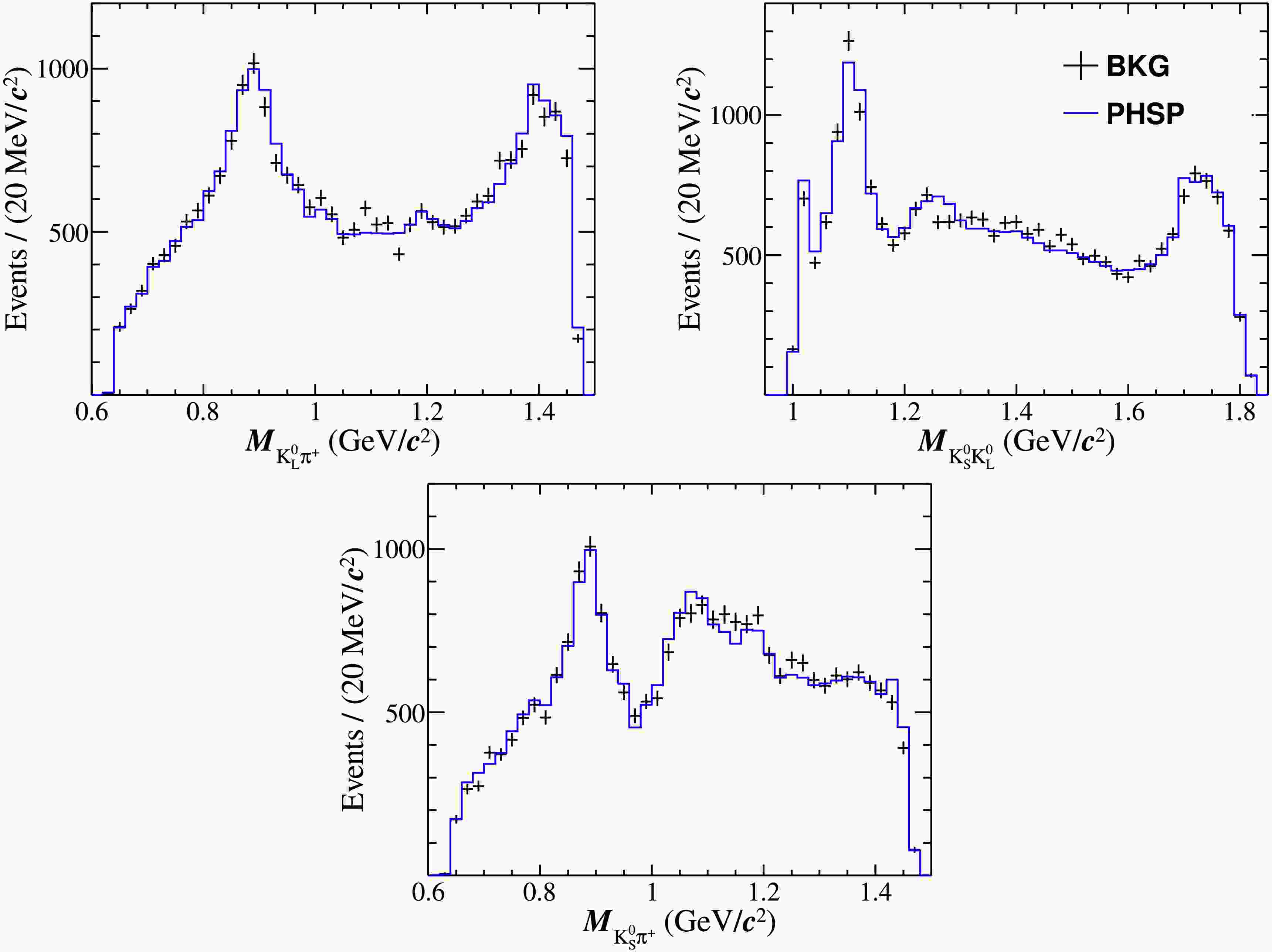
To capture the complex multidimensional correlations and dynamic structures within the phase space, a comprehensive set of kinematic variables is provided to the XGBoost algorithm. Further, to ensure the optimal performance of the decision trees, the number of input features exceeds the absolute independent kinematic degrees of freedom of the decay. As an illustrative example, Fig. 1 compares the kinematic projections of a simulated background sample for $ D_s^+ \to K_S^0 K_L^0 \pi^+ $ [7] against the learned background distribution $ {\cal{B}}_\epsilon $ modeled by the XGBoost classifier.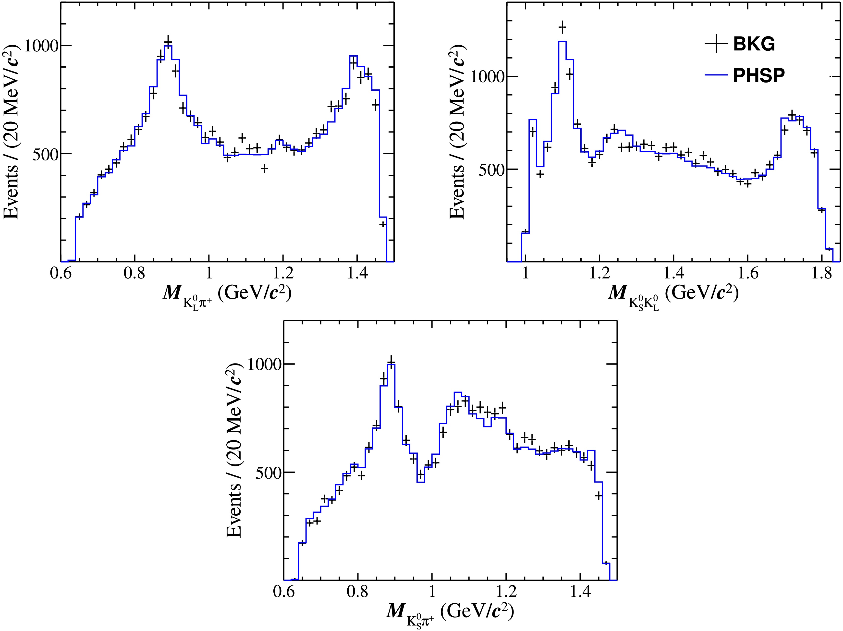

Figure 1.  (color online) Projections of a background MC sample for $ D_s^+ \to K_S^0 K_L^0 \pi^+ $ and the corresponding background shape obtained from XGBoost trained on that sample. Background shape projections are made by drawing the distributions of a reconstructed MC sample with $ P_{\rm {BKG}}/P_{\rm {PHSP}} $ as weight.

Visualizing the agreement between the data and fitted model through one-dimensional projections onto physical observables, such as invariant masses, decay angles, and particle momenta, provides the most intuitive means to assess fit quality and clarify the underlying physics. However, analytically constructing these expected projections directly from the fitted parameters is highly nontrivial. The dynamical amplitude must be convolved with the kinematic PHSP factor $ R(p) $ and detector efficiency $ \epsilon(p) $. Unfortunately, explicit analytical forms for these detector and kinematic effects are intractable and highly dependent on the choice of coordinates.

In practice, this challenge is circumvented by utilizing a fully reconstructed PHSP MC sample. The expected distribution of the fit result for any given physical observable is constructed by filling a histogram with reconstructed PHSP MC events, wherein each event is weighted by its fitted dynamical amplitude squared $ |{\cal{M}}(p)|^2 $. The reconstructed PHSP MC sample inherently encapsulates both the kinematic PHSP boundaries and detector efficiency, and therefore, these critical effects are naturally integrated into the resulting projected distributions without requiring explicit analytical modeling.

The raw outputs of an amplitude analysis are the relative magnitudes and phases of intermediate dynamic amplitudes. However, these parameters inherently depend on the selected normalization and phase conventions of the specific amplitude formalism. Consequently, variations in the amplitude parametrization can significantly alter the fitted parameter values. To enable robust comparisons with independent measurements and provide meaningful inputs for theoretical phenomenologists, one must extract formalism-independent physical quantities. These quantities, referred to as fit fractions, represent the relative contribution of each individual intermediate process to the total multibody decay rate. Owing to the quantum interference between intermediate decay channels, the sum of all fit fractions does not necessarily equal unity; the sum will be less than unity in the presence of net constructive interference and greater than unity for net destructive interference.

The specific fit fraction for the $ n^{\mathrm{th}} $ intermediate process is defined as

Fit fractions represent pure, post-decay physical quantities; therefore, this definition intentionally isolates the underlying dynamics from detector acceptance and resolution effects, fundamentally distinguishing it from the experimentally measured signal PDF $ f_S(p) $. In practice, the integral in Eq. (13) is evaluated numerically via MC integration using a generator-level PHSP MC sample (i.e., prior to any detector simulation).

where $ N_{\mathrm{gen}} $ and $ p_k $ represent the total number of generator-level PHSP MC events and kinematics of the $ k^{\mathrm{th}} $ generated event, respectively. The interference fraction between the $ n^{\mathrm{th}} $ and $ m^{\mathrm{th}} $ amplitudes is derived analogously as

Evaluating the statistical uncertainties of these fit fractions is a highly complex task because analytically propagating the uncertainties from fitted magnitudes and phases is practically unfeasible because of the severe nonlinearities and parameter correlations. The standard approach to address this is to perform the MC sampling of the fit parameters based on their full covariance matrix (obtained from the fit convergence). This pseudoexperiment procedure generates an empirical distribution for each fit fraction. These distributions are fitted with a Gaussian function, and the resulting width is assigned as statistical uncertainty.

However, it is crucial to recognize that these distributions are not guaranteed to be strictly Gaussian. Strong interference effects or the proximity to physical boundaries (e.g., fit fractions near 0% or 100%) can heavily skew the distributions. In such asymmetric scenarios, a Gaussian approximation is fundamentally inadequate. An asymmetric Gaussian or a Poisson distribution would be more appropriate.

The mathematical formulation and coordinate representation of decay amplitudes are inherently dictated by the underlying physical dynamics of the specific process. This section outlines the formalisms implemented for both hadronic and semileptonic charmed-meson decays at BESIII, including the established parametrizations of intermediate resonance propagators.

The amplitude analyses of hadronic charmed-meson decays at BESIII employ the isobar model within the covariant tensor formalism [8], utilizing the four-momenta of the final-state particles as fundamental kinematic variables. In the isobar model, a multibody decay is conceptualized as a coherent sum of various intermediate quasi-two-body transitions (see Eq. (2)).

In a three-body decay, the topological structure typically proceeds via the initial D meson decaying into an intermediate resonance and a bachelor particle, with the resonance subsequently decaying into the remaining two final-state particles. The dynamic amplitude $ {\cal{A}}_n $ for such an intermediate process is modeled as

where $ S_n $ represents the spin-projection factor; $ F_n^r $ and $ F_n^{D} $ are the Blatt-Weisskopf barrier factors for the intermediate resonance and mother D meson, respectively; and $ P_n $ represents the resonance propagator that mathematically describes its mass lineshape.

For four-body decays, the intermediate processes are generally classified into two topological categories: quasi-two-body and cascade. In a quasi-two-body process, the D meson decays into two primary resonance states, each of which subsequently decays into two final-state particles. In a cascade process, the D meson decays into a primary resonance and a bachelor particle; this primary resonance subsequently decays into a secondary resonance and another final-state particle, and the secondary resonance ultimately decays into the final particle pair. In both topologies, the amplitude $ {\cal{A}}_n $ is parametrized as

where superscripts $ r_1 $ and $ r_2 $ denote the first and second intermediate resonances, respectively. Explicit formulations of spin factors and Blatt-Weisskopf barriers for arbitrary spin configurations are detailed in Ref. [8]. The distinct propagator forms for frequently observed resonances are outlined in Section III.C. To satisfy Bose symmetry, the total amplitude $ {\cal{A}}_n $ must be explicitly symmetrized under the exchange of any identical final-state bosons. Furthermore, assuming strict $\rm CP$ conservation, the amplitude for a $ \bar{D} $ decay is mathematically identical to the D decay amplitude evaluated at the $\rm CP$-conjugate phase-space point. In practical data analysis, this implies that, when fitting a $ \bar{D} $ data sample, the spatial momenta ($ \vec{p} $) of all final-state particles must be inverted ($ \vec{p} \to -\vec{p} $) prior to amplitude evaluation.

Any combination of two or three final-state particles can theoretically form a resonant state, and this can manifest as a scalar, pseudoscalar, vector, axial-vector, or tensor. However, the physical realization of these intermediate processes is strictly constrained by fundamental quantum selection rules, predominantly angular-momentum conservation. Although the initial weak D-meson decay intrinsically violates parity, the subsequent resonance decays proceed via strong or electromagnetic interactions where parity is strictly conserved. By rigorously examining the quantum numbers ($ J^{PC} $) of the intermediate states, one can systematically deduce the allowed and forbidden transition paths. In practice, a comprehensive suite of kinematically allowed intermediate processes must be empirically evaluated in the fit, thereby utilizing the specific spin factors and Blatt-Weisskopf barriers appropriate for the corresponding orbital angular momenta and resonance species.

The theoretical formulation of semileptonic decays naturally factorizes into leptonic and hadronic currents. The dynamics of these two currents can be rigorously separated because there are no final-state strong interactions between the leptonic and hadronic systems [9]. Consequently, the differential decay amplitude for a $ D \to M_{1}M_{2}\ell^+\nu_{\ell} $ transition (where $ M_{1,2} $ denote mesons and $ \ell=e,\mu $) is naturally parametrized by five independent kinematic variables: the squared invariant masses of the hadronic ($ m^2 $) and leptonic ($ q^2 $) systems, their respective helicity angles ($ \theta_M $ and $ \theta_\ell $), and the angle (χ) between their respective decay planes. Squaring the amplitude and incorporating the phase-space kinematics yields the fully differential decay rate (analogous to the $ |{\cal{M}}|^2 R(p)\mathrm{d}p $ term in Eq. (6)), which is expressed as

where $ X\beta_{M}\beta_{\ell} $ represents the kinematic phase-space factor. Here, $ X=p_{MM}m_{D} $, where $ p_{MM} $ represents the magnitude of the three momenta of the $ M_1M_2 $ system evaluated in the D-meson rest frame, and $ m_{D} $ represents the D-meson mass. The factors $ \beta_{M}=2p_{M}/m $ and $ \beta_{\ell}=2p_{\ell}/q $ incorporate the momentum magnitudes $ p_{M} $ and $ p_{\ell} $ of $ M_{1} $ and $ \ell^+ $ evaluated in their respective $ M_{1}M_{2} $ and $ \ell^{+}\nu_{\ell} $ center-of-mass frames.

The decay intensity $ {\cal{I}} $ (corresponding to the $ |{\cal{M}}|^2 $ term in Eq. (6)) contains the core dynamic information. It is conventionally decomposed in terms of the angular variables $ \cos\theta_{\ell} $ and χ to mathematically isolate the substructure of the hadronic system. This intensity encapsulates the complex hadronic form factors, which are systematically expanded in partial waves based on the angular momentum of the $ M_1M_2 $ pair. Under the assumption of $\rm CP$ conservation, the amplitude for the charge-conjugate $ \bar{D} $ decay is obtained by reversing the sign of the azimuthal angle ($ \chi \to -\chi $), while the other four kinematic variables remain invariant. A comprehensive parametrization of this theoretical framework is detailed in Ref. [9]. The specific parametrizations of the intermediate hadronic resonance propagators are discussed in the subsequent section.

Propagators parameterize the mass lineshapes of intermediate resonances. The selection of propagator model for a given resonance depends on its width, its proximity to decay thresholds, and possible presence of overlapping states with the same quantum numbers. This section summarizes the parameterizations employed in the amplitude analyses of charmed-meson decays.

A relativistic Breit-Wigner (RBW) propagator provides an adequate description for most isolated resonances that are narrow and far from the decay thresholds [10]. Resonances commonly parameterized in this way include ω, ϕ, $ b_1(1235) $, $ a_1(1260) $, $ f_2(1270) $, $ a_2(1320) $, $ f_0(1370) $, $ \eta(1405) $, $ a_0(1450) $, $ f_0(1500) $, $ K^*(892) $, $ K_1(1270) $, $ K_1(1400) $, and $ K_2^*(1430) $.

The general form of a RBW propagator is

where $ s = m^2 $ represents the invariant mass squared of decay products. For a two-body decay, the energy-dependent width is given by

where $ m_0 $ and $ \Gamma_0 $ represent the mass and width of the intermediate resonance, respectively. They can be fixed to their known values [1]. The quantity q is the magnitude of the breakup momentum of the daughter particles in the resonance rest frame $ q_0 = q(s=m_0^2) $, and $ F_L $ represents the Blatt-Weisskopf barrier factor for orbital angular momentum L; their explicit definitions can be found in Ref. [1]. For axial-vector mesons such as $ a_1(1260) $, $ K_1(1270) $, and $ K_1(1400) $, which decay predominantly through three-body processes, a more general mass-dependent width $ \Gamma(s) $ should be used; further details can be found in Ref. [11].

For broad vector resonances such as $ \rho(770) $ and $ \rho(1450) $, a simple RBW form fails to describe the lineshape near threshold accurately. In these cases, the Gounaris-Sakurai (GS) parametrization [12] is adopted, which imposes analyticity constraints on the $ \pi\pi $ P-wave amplitude.

The function $ f(s) $ and constant d are defined in Ref. [12]; $ d = f(0)/(\Gamma_0 m_0) $ is fixed by the normalization at $ s=0 $. In certain cases, the $ \pi^+\pi^- $ mass spectrum in the $ \rho(770) $ region cannot be adequately described by the GS lineshape alone becase of distortions induced by $ \rho-\omega $ mass mixing. When these effects are significant, a ρ–ω mixing lineshape [13] should be adopted to account for the interference.

The $ \sigma/f_0(500) $ is a very broad scalar resonance with strong coupling to multiple channels. Its propagator is parameterized following Ref. [14] as

with $ \Gamma_{\text{tot}}(s) = g_1 \dfrac{\rho_{\pi\pi}(s)}{\rho_{\pi\pi}(m_0^2)} + g_2 \dfrac{\rho_{4\pi}(s)}{\rho_{4\pi}(m_0^2)} $. Here, $ \rho_{\pi\pi}(s) $ and $ \rho_{4\pi}(s) $ represent the Lorentz-invariant phase-space factors for the two-pion and four-pion channels, and $ g_{1,2} $ are the corresponding coupling constants. Their detailed parametrizations and numerical values are taken from Ref. [15].

$ f_0(980) $ couples strongly to $ \pi\pi $ and $ K\bar{K} $, and it lies just below the $ K\bar{K} $ mass threshold. A Flatté formula [16] is therefore used to address the threshold effect.

where $ \rho_{\pi\pi}(s) $ and $ \rho_{K\bar{K}}(s) $ represent the Lorentz-invariant PHSP factors, and $ g_{1,2} $ represents their coupling constants. Their definitions can be found in Ref. [16]. Below the $ K\bar{K} $ threshold, the analytic continuation $\sqrt{1-4m_K^2/s} \to {\rm i}\sqrt{4m_K^2/s-1}$ is applied. The parameters can be fixed to the values reported in Ref. [16].

The $ a_0(980) $ couples strongly to $ \pi\eta $ and $ K\bar{K} $, and it lies close to the $ K\bar{K} $ threshold, requiring a coupled-channel treatment [17−20]. Two parameterizations are considered. The first is a Flatté form [21]

where $ g_j $ and $ \rho_j(s) $ represent the coupling constant and PHSP factor for channel j, respectively. This retains only the imaginary part of the self-energy, and it is adequate when the PHSP varies slowly and no sharp thresholds lie near the resonance peak.

The second is a dispersive approach [22, 23], which includes the full complex self-energy $\Pi_j(s) = \text{Re}\,\Pi_j(s) + {\rm i}\,\text{Im}\,\Pi_j(s)$.

The imaginary part is given by $ \text{Im}\,\Pi_j(s) = \rho_j(s) F_j^2(s) $, where $ F_j(s) $ represents a form factor [22]. The real part is obtained from the dispersion relationship

This formulation naturally considers the prominent cusp at the $ K\bar{K} $ threshold. The parameters can be fixed to those in Ref. [23].

For the $ \pi^+\pi^- $ and $ \pi^0\pi^0 $ S-waves, multiple broad and overlapping resonances appear, and a simple sum of Breit-Wigner propagators violate unitarity. In such cases, a K-matrix parametrization [24, 25] is adopted. The amplitude is expressed as

where I, K, and ρ represent the identity, scattering, and phase-space matrices, respectively. The indices $ i,j $ label the coupled channels $ 1 = \pi\pi $, $ 2 = K\bar{K} $, $ 3 = 4\pi $, $ 4 = \eta\eta $, and $ 5 = \eta\eta' $. The production vector P is parametrized as

All parameters not explicitly defined here (including the K-matrix elements, $ f_{1j}^{\rm{prod}} $, $ \beta^{\alpha} $, $ s_0^{\rm{scatt}} $, $ g_j^{\alpha} $, and $ m_{\alpha} $) are taken from the literature [24, 25]. Although the scattering K-matrix is fixed based on independent scattering data, the production parameters $ f_{1j}^{\rm{prod}} $ and $ \beta^{\alpha} $ are process-dependent and left free in the fit.

For the $ K\pi $ S-wave, two complementary parametrizations are employed. The LASS model [25] describes the amplitude as a coherent sum of a $ K_0^*(1430) $ Breit-Wigner resonance [1] and an effective-range nonresonant component.

where F ($ \phi_F $) and R ($ \phi_R $) represent the magnitudes (phases) for the nonresonant and resonant terms. Their relative phase is fixed by Watson's theorem, which makes this model well suited for the low-mass region where inelastic channels are negligible. For analyses covering a wider energy range where coupled-channel effects become important, a K-matrix model [26] is also employed. This model splits the amplitude into isospin components $ {\cal{A}}_{1/2} $ and $ {\cal{A}}_{3/2} $, treating resonant and nonresonant contributions on the same footing and guaranteeing unitarity with all relevant coupled channels. The parameters can be cited from Ref. [27].

Amplitude analysis serves as a robust analytical framework that bridges the gap between experimental measurements and theoretical phenomenologies, thereby enabling the extraction of fundamental two-body intermediate dynamics from complex multibody final states. In this study, we provided a comprehensive review of the amplitude-analysis methodologies employed for charmed-meson decays at the BESIII experiment with a strong emphasis on practical experimental implementation. We detailed the construction of the likelihood functions, utilization of MC integration for strict normalization, treatment of detector efficiencies and finite resolutions, and modeling of backgrounds via multidimensional reweighting techniques. Furthermore, we outlined the specific amplitude formalisms governing both hadronic and semileptonic decays, including the standard parametrizations for intermediate resonance propagators.

The practical execution of amplitude analysis relies critically on dedicated MC simulations. The selection of a specific MC sample is intrinsically tied to the analytical task guided by a clear functional mapping: a generator-level PHSP MC sample strictly represents the pure kinematic phase-space boundary; a fully reconstructed PHSP MC sample naturally folds in the detector acceptance and efficiency; and a reconstructed signal MC sample further encapsulates the empirical detector resolution effects. Consequently, mapping a theoretical amplitude model onto observable data projections necessitates a reconstructed MC sample, whereas the extraction of purely physical fit fractions for intermediate processes strictly requires a generator-level PHSP MC sample.

Leveraging these comprehensive methodologies, the BESIII Collaboration determined the branching fractions for key charmed-meson decays [7, 28−34], including pivotal channels such as $ D \to K^{*}\pi $ [29, 34] and $ D_s \to \phi\pi $ [7, 32]. These results provide crucial experimental constraints on the nonperturbative dynamics of quantum chromodynamics. The branching fractions of decays involving scalar and axial-vector mesons have also been precisely measured [35−40]. Theoretical predictions for decays involving scalar mesons are highly sensitive to their assumed internal quark structures, such as conventional $ q\bar{q} $ states versus tetraquark configurations [17, 18, 41, 42]. For decays involving axial-vector $ K_1 $ mesons, predictions vary widely as well, because of the strong dependence on both the selected theoretical approach and the poorly constrained $ K_1 $ mixing angle [43]. These theoretical difficulties and the scarcity of reliable predictions make experimental inputs essential for clarifying the underlying dynamics. Beyond branching fractions, amplitude analyses have enabled the extraction of complex polarization observables in $ D \to VV $ decays [44−46] and the precise determination of the $\rm CP$-even fractions in $ D^0 $ multibody decays. Moreover, systematic comparisons across these multibody channels enable independent determinations of absolute ϕ-meson decay branching fractions [7, 32, 47]. By performing simultaneous amplitude fits across multiple coupled decay channels, we uniquely probe $ K_S^0 $–$ K_L^0 $ asymmetries [7], evaluate U-spin symmetry breaking, and explore fundamental quantum correlations within the neutral $ D^0 $ system.

The BESIII experiment has accumulated unprecedented charmonium threshold data samples corresponding to an integrated luminosity of $ 20.3\; \mathrm{fb}^{-1} $ at $ \sqrt{s}=3.773\; \mathrm{GeV} $ [3] and an additional $ 7.33\; \mathrm{fb}^{-1} $ in the energy range between $ 4.128 $ and $ 4.226\; \mathrm{GeV} $. Capitalizing on these massive datasets, a new generation of high-precision amplitude analyses is currently underway. We anticipate a significant amount of groundbreaking results, including unparalleled precision in branching fractions, deeper resolution of broad resonant structures and polarizations, and stringent tests of fundamental symmetries. These results are expected to collectively and significantly advance our understanding of charm-decay dynamics.