


 Abstract
 HTML
HTML Reference
 Related
 PDF
PDF


-
Nuclear density functional theory (DFT) provides a microscopic and self-consistent framework for a unified description of finite nuclei and neutron-star matter based on a universal energy density functional (EDF) [1−4]. In its simplest implementation, namely the self-consistent mean-field approximation, the complex nuclear many-body problem is effectively reduced to an equivalent one-body problem. The energy of a nuclear system is then approximated as a functional of the powers and gradients of nuclear densities and currents. According to the Kohn-Sham scheme [5], this functional can be represented in terms of auxiliary single-particle wave functions. This approach, known as single-reference (SR)-DFT, has achieved great success in reproducing the properties of nuclear matter around saturation density and the ground states of finite nuclei across the entire nuclear chart [6−10].
Despite its success, nuclear DFT faces significant challenges arising from discrepancies among predictions made by different EDFs. These discrepancies lead to considerable uncertainties, particularly for the equation of state of nuclear matter at densities far from the saturation point [11], and for neutron-rich nuclei with limited experimental data [12]. In this context, it is necessary to quantify the errors of nuclear DFT, which consist of systematic and statistical components [13]. Because widely used nuclear EDFs are derived from phenomenological nucleon-nucleon effective interactions—such as non-relativistic Skyrme [14, 15] and Gogny [16, 17] forces, as well as relativistic covariant EDFs [18−21]—it is difficult to quantify the systematic errors of nuclear DFT. This remains the case despite efforts to develop new generations of EDFs [22−31] inspired by effective field theories or based on ab initio calculations, as reviewed in [4, 32−34]. In contrast, the statistical error associated with a given EDF, which arises from variations in the parameters around their optimal values, can be quantified using statistical methods. Over the past decade, significant progress has been made in quantifying the statistical uncertainties of DFT predictions for nuclear ground-state bulk properties [9, 13, 35−37], and in identifying potential correlations between nuclear matter properties [38] and neutron-star observables [39, 40].
Extending DFT to study energy spectra and transition strengths of nuclear low-lying states typically requires going beyond the mean-field approximation. In SR-DFT, the nuclear wave function is approximated as a product of auxiliary single-particle wave functions determined from the variational principle. This approach ensures that the solution corresponds to a local energy minimum within the restricted Hilbert space, but it does not preserve the symmetry structure of nuclear many-body Hamiltonians. In SR-DFT for open-shell nuclei, the introduction of deformation and pairing correlations violates the
$ SO(3) $ and$ U(1) $ symmetries. As a result, the nuclear wave functions lack the good quantum numbers associated with angular momentum and particle number, which are critical for studies of nuclear low-lying spectroscopy [41]. The restoration of broken symmetries and the inclusion of dynamical correlations from fluctuations around the equilibrium shape in SR-DFT can be achieved through quantum-number projection and the generator coordinate method (GCM) [41, 42]. This extended framework, known as multireference DFT (MR-DFT), has been successfully applied to study nuclear low-lying states [1, 43−50], as well as the nuclear matrix elements (NMEs) of$ 0\nu\beta\beta $ decay [51−54].With advances in nuclear technology and methodologies, nuclear physics is entering an era of high precision. Accurate measurements of atomic and nuclear spectroscopy in neutron-rich nuclei [55, 56], as well as the half-lives of rare nuclear processes [57−59], require precise modeling of nuclear low-lying states and the corresponding NMEs. Therefore, quantifying the theoretical uncertainties of these physical quantities is essential for making meaningful comparisons with other models and available data. However, uncertainties in nuclear low-lying states have been scarcely studied within EDF frameworks, primarily because of the substantial computational cost of repeated calculations using varying EDF parameter sets.
Recently, we performed a Bayesian analysis of nuclear low-lying states and
$ 0\nu\beta\beta $ decay within a covariant EDF framework, enabled by the newly developed subspace-projected covariant density functional theory (SP-CDFT) [60]. This approach combines multireference CDFT (MR-CDFT) with the eigenvector continuation (EC) method. The central idea of EC is to represent the eigenvector of a target Hamiltonian within a low-dimensional subspace spanned by the eigenvectors of a set of sampling Hamiltonians [61]. The efficiency and accuracy of EC, when coupled with various many-body methods, have been demonstrated in a wide range of toy models [62−66] as well as in nuclear structure and reaction studies [67−73]; see also the reviews [74, 75]. In the present work, we provide a detailed description of this framework and apply it to quantify statistical uncertainties in both nuclear matter properties and low-lying nuclear states within a Bayesian framework. For illustration, we consider candidate nuclei for$ 0\nu\beta\beta $ decay and their daughter nuclei, including 150Nd and 150Sm, as well as 136Xe and 136Ba. The former pair is well deformed, whereas the latter pair is spherical or weakly deformed. Comparing the predictions with their associated statistical uncertainties provides valuable insight into the strengths and limitations of the current implementation of MR-CDFT.The remainder of this paper is organized as follows. In Sec. II, we introduce the theoretical framework, including SR-CDFT, MR-CDFT, and SP-CDFT. Section III presents benchmark calculations and the quantification of statistical uncertainties for nuclear matter and low-lying nuclear states. Finally, Sec. IV summarizes our findings and outlines future perspectives.
-
Nuclear density functional theory (DFT) provides a microscopic and self-consistent framework for a unified description of finite nuclei and neutron-star matter based on a universal energy density functional (EDF) [1−4]. In its simplest implementation, namely the self-consistent mean-field approximation, the complex nuclear many-body problem is effectively reduced to an equivalent one-body problem. The energy of a nuclear system is then approximated as a functional of the powers and gradients of nuclear densities and currents. According to the Kohn-Sham scheme [5], this functional can be represented in terms of auxiliary single-particle wave functions. This approach, known as single-reference (SR)-DFT, has achieved great success in reproducing the properties of nuclear matter around saturation density and the ground states of finite nuclei across the entire nuclear chart [6−10].
Despite its success, nuclear DFT faces significant challenges arising from discrepancies among predictions made by different EDFs. These discrepancies lead to considerable uncertainties, particularly for the equation of state of nuclear matter at densities far from the saturation point [11], and for neutron-rich nuclei with limited experimental data [12]. In this context, it is necessary to quantify the errors of nuclear DFT, which consist of systematic and statistical components [13]. Because widely used nuclear EDFs are derived from phenomenological nucleon-nucleon effective interactions—such as non-relativistic Skyrme [14, 15] and Gogny [16, 17] forces, as well as relativistic covariant EDFs [18−21]—it is difficult to quantify the systematic errors of nuclear DFT. This remains the case despite efforts to develop new generations of EDFs [22−31] inspired by effective field theories or based on ab initio calculations, as reviewed in [4, 32−34]. In contrast, the statistical error associated with a given EDF, which arises from variations in the parameters around their optimal values, can be quantified using statistical methods. Over the past decade, significant progress has been made in quantifying the statistical uncertainties of DFT predictions for nuclear ground-state bulk properties [9, 13, 35−37], and in identifying potential correlations between nuclear matter properties [38] and neutron-star observables [39, 40].
Extending DFT to study energy spectra and transition strengths of nuclear low-lying states typically requires going beyond the mean-field approximation. In SR-DFT, the nuclear wave function is approximated as a product of auxiliary single-particle wave functions determined from the variational principle. This approach ensures that the solution corresponds to a local energy minimum within the restricted Hilbert space, but it does not preserve the symmetry structure of nuclear many-body Hamiltonians. In SR-DFT for open-shell nuclei, the introduction of deformation and pairing correlations violates the
$ SO(3) $ and$ U(1) $ symmetries. As a result, the nuclear wave functions lack the good quantum numbers associated with angular momentum and particle number, which are critical for studies of nuclear low-lying spectroscopy [41]. The restoration of broken symmetries and the inclusion of dynamical correlations from fluctuations around the equilibrium shape in SR-DFT can be achieved through quantum-number projection and the generator coordinate method (GCM) [41, 42]. This extended framework, known as multireference DFT (MR-DFT), has been successfully applied to study nuclear low-lying states [1, 43−50], as well as the nuclear matrix elements (NMEs) of$ 0\nu\beta\beta $ decay [51−54].With advances in nuclear technology and methodologies, nuclear physics is entering an era of high precision. Accurate measurements of atomic and nuclear spectroscopy in neutron-rich nuclei [55, 56], as well as the half-lives of rare nuclear processes [57−59], require precise modeling of nuclear low-lying states and the corresponding NMEs. Therefore, quantifying the theoretical uncertainties of these physical quantities is essential for making meaningful comparisons with other models and available data. However, uncertainties in nuclear low-lying states have been scarcely studied within EDF frameworks, primarily because of the substantial computational cost of repeated calculations using varying EDF parameter sets.
Recently, we performed a Bayesian analysis of nuclear low-lying states and
$ 0\nu\beta\beta $ decay within a covariant EDF framework, enabled by the newly developed subspace-projected covariant density functional theory (SP-CDFT) [60]. This approach combines multireference CDFT (MR-CDFT) with the eigenvector continuation (EC) method. The central idea of EC is to represent the eigenvector of a target Hamiltonian within a low-dimensional subspace spanned by the eigenvectors of a set of sampling Hamiltonians [61]. The efficiency and accuracy of EC, when coupled with various many-body methods, have been demonstrated in a wide range of toy models [62−66] as well as in nuclear structure and reaction studies [67−73]; see also the reviews [74, 75]. In the present work, we provide a detailed description of this framework and apply it to quantify statistical uncertainties in both nuclear matter properties and low-lying nuclear states within a Bayesian framework. For illustration, we consider candidate nuclei for$ 0\nu\beta\beta $ decay and their daughter nuclei, including 150Nd and 150Sm, as well as 136Xe and 136Ba. The former pair is well deformed, whereas the latter pair is spherical or weakly deformed. Comparing the predictions with their associated statistical uncertainties provides valuable insight into the strengths and limitations of the current implementation of MR-CDFT.The remainder of this paper is organized as follows. In Sec. II, we introduce the theoretical framework, including SR-CDFT, MR-CDFT, and SP-CDFT. Section III presents benchmark calculations and the quantification of statistical uncertainties for nuclear matter and low-lying nuclear states. Finally, Sec. IV summarizes our findings and outlines future perspectives.
-
Nuclear density functional theory (DFT) provides a microscopic and self-consistent framework for a unified description of finite nuclei and neutron-star matter based on a universal energy density functional (EDF) [1−4]. In its simplest implementation, namely the self-consistent mean-field approximation, the complex nuclear many-body problem is effectively reduced to an equivalent one-body problem. The energy of a nuclear system is then approximated as a functional of the powers and gradients of nuclear densities and currents. According to the Kohn-Sham scheme [5], this functional can be represented in terms of auxiliary single-particle wave functions. This approach, known as single-reference (SR)-DFT, has achieved great success in reproducing the properties of nuclear matter around saturation density and the ground states of finite nuclei across the entire nuclear chart [6−10].
Despite its success, nuclear DFT faces significant challenges arising from discrepancies among predictions made by different EDFs. These discrepancies lead to considerable uncertainties, particularly for the equation of state of nuclear matter at densities far from the saturation point [11], and for neutron-rich nuclei with limited experimental data [12]. In this context, it is necessary to quantify the errors of nuclear DFT, which consist of systematic and statistical components [13]. Because widely used nuclear EDFs are derived from phenomenological nucleon-nucleon effective interactions—such as non-relativistic Skyrme [14, 15] and Gogny [16, 17] forces, as well as relativistic covariant EDFs [18−21]—it is difficult to quantify the systematic errors of nuclear DFT. This remains the case despite efforts to develop new generations of EDFs [22−31] inspired by effective field theories or based on ab initio calculations, as reviewed in [4, 32−34]. In contrast, the statistical error associated with a given EDF, which arises from variations in the parameters around their optimal values, can be quantified using statistical methods. Over the past decade, significant progress has been made in quantifying the statistical uncertainties of DFT predictions for nuclear ground-state bulk properties [9, 13, 35−37], and in identifying potential correlations between nuclear matter properties [38] and neutron-star observables [39, 40].
Extending DFT to study energy spectra and transition strengths of nuclear low-lying states typically requires going beyond the mean-field approximation. In SR-DFT, the nuclear wave function is approximated as a product of auxiliary single-particle wave functions determined from the variational principle. This approach ensures that the solution corresponds to a local energy minimum within the restricted Hilbert space, but it does not preserve the symmetry structure of nuclear many-body Hamiltonians. In SR-DFT for open-shell nuclei, the introduction of deformation and pairing correlations violates the
$ SO(3) $ and$ U(1) $ symmetries. As a result, the nuclear wave functions lack the good quantum numbers associated with angular momentum and particle number, which are critical for studies of nuclear low-lying spectroscopy [41]. The restoration of broken symmetries and the inclusion of dynamical correlations from fluctuations around the equilibrium shape in SR-DFT can be achieved through quantum-number projection and the generator coordinate method (GCM) [41, 42]. This extended framework, known as multireference DFT (MR-DFT), has been successfully applied to study nuclear low-lying states [1, 43−50], as well as the nuclear matrix elements (NMEs) of$ 0\nu\beta\beta $ decay [51−54].With advances in nuclear technology and methodologies, nuclear physics is entering an era of high precision. Accurate measurements of atomic and nuclear spectroscopy in neutron-rich nuclei [55, 56], as well as the half-lives of rare nuclear processes [57−59], require precise modeling of nuclear low-lying states and the corresponding NMEs. Therefore, quantifying the theoretical uncertainties of these physical quantities is essential for making meaningful comparisons with other models and available data. However, uncertainties in nuclear low-lying states have been scarcely studied within EDF frameworks, primarily because of the substantial computational cost of repeated calculations using varying EDF parameter sets.
Recently, we performed a Bayesian analysis of nuclear low-lying states and
$ 0\nu\beta\beta $ decay within a covariant EDF framework, enabled by the newly developed subspace-projected covariant density functional theory (SP-CDFT) [60]. This approach combines multireference CDFT (MR-CDFT) with the eigenvector continuation (EC) method. The central idea of EC is to represent the eigenvector of a target Hamiltonian within a low-dimensional subspace spanned by the eigenvectors of a set of sampling Hamiltonians [61]. The efficiency and accuracy of EC, when coupled with various many-body methods, have been demonstrated in a wide range of toy models [62−66] as well as in nuclear structure and reaction studies [67−73]; see also the reviews [74, 75]. In the present work, we provide a detailed description of this framework and apply it to quantify statistical uncertainties in both nuclear matter properties and low-lying nuclear states within a Bayesian framework. For illustration, we consider candidate nuclei for$ 0\nu\beta\beta $ decay and their daughter nuclei, including 150Nd and 150Sm, as well as 136Xe and 136Ba. The former pair is well deformed, whereas the latter pair is spherical or weakly deformed. Comparing the predictions with their associated statistical uncertainties provides valuable insight into the strengths and limitations of the current implementation of MR-CDFT.The remainder of this paper is organized as follows. In Sec. II, we introduce the theoretical framework, including SR-CDFT, MR-CDFT, and SP-CDFT. Section III presents benchmark calculations and the quantification of statistical uncertainties for nuclear matter and low-lying nuclear states. Finally, Sec. IV summarizes our findings and outlines future perspectives.
-
Nuclear density functional theory (DFT) provides a microscopic and self-consistent framework for a unified description of finite nuclei and neutron-star matter based on a universal energy density functional (EDF) [1−4]. In its simplest implementation, namely the self-consistent mean-field approximation, the complex nuclear many-body problem is effectively reduced to an equivalent one-body problem. The energy of a nuclear system is then approximated as a functional of the powers and gradients of nuclear densities and currents. According to the Kohn-Sham scheme [5], this functional can be represented in terms of auxiliary single-particle wave functions. This approach, known as single-reference (SR)-DFT, has achieved great success in reproducing the properties of nuclear matter around saturation density and the ground states of finite nuclei across the entire nuclear chart [6−10].
Despite its success, nuclear DFT faces significant challenges arising from discrepancies among predictions made by different EDFs. These discrepancies lead to considerable uncertainties, particularly for the equation of state of nuclear matter at densities far from the saturation point [11], and for neutron-rich nuclei with limited experimental data [12]. In this context, it is necessary to quantify the errors of nuclear DFT, which consist of systematic and statistical components [13]. Because widely used nuclear EDFs are derived from phenomenological nucleon-nucleon effective interactions—such as non-relativistic Skyrme [14, 15] and Gogny [16, 17] forces, as well as relativistic covariant EDFs [18−21]—it is difficult to quantify the systematic errors of nuclear DFT. This remains the case despite efforts to develop new generations of EDFs [22−31] inspired by effective field theories or based on ab initio calculations, as reviewed in [4, 32−34]. In contrast, the statistical error associated with a given EDF, which arises from variations in the parameters around their optimal values, can be quantified using statistical methods. Over the past decade, significant progress has been made in quantifying the statistical uncertainties of DFT predictions for nuclear ground-state bulk properties [9, 13, 35−37], and in identifying potential correlations between nuclear matter properties [38] and neutron-star observables [39, 40].
Extending DFT to study energy spectra and transition strengths of nuclear low-lying states typically requires going beyond the mean-field approximation. In SR-DFT, the nuclear wave function is approximated as a product of auxiliary single-particle wave functions determined from the variational principle. This approach ensures that the solution corresponds to a local energy minimum within the restricted Hilbert space, but it does not preserve the symmetry structure of nuclear many-body Hamiltonians. In SR-DFT for open-shell nuclei, the introduction of deformation and pairing correlations violates the
$ SO(3) $ and$ U(1) $ symmetries. As a result, the nuclear wave functions lack the good quantum numbers associated with angular momentum and particle number, which are critical for studies of nuclear low-lying spectroscopy [41]. The restoration of broken symmetries and the inclusion of dynamical correlations from fluctuations around the equilibrium shape in SR-DFT can be achieved through quantum-number projection and the generator coordinate method (GCM) [41, 42]. This extended framework, known as multireference DFT (MR-DFT), has been successfully applied to study nuclear low-lying states [1, 43−50], as well as the nuclear matrix elements (NMEs) of$ 0\nu\beta\beta $ decay [51−54].With advances in nuclear technology and methodologies, nuclear physics is entering an era of high precision. Accurate measurements of atomic and nuclear spectroscopy in neutron-rich nuclei [55, 56], as well as the half-lives of rare nuclear processes [57−59], require precise modeling of nuclear low-lying states and the corresponding NMEs. Therefore, quantifying the theoretical uncertainties of these physical quantities is essential for making meaningful comparisons with other models and available data. However, uncertainties in nuclear low-lying states have been scarcely studied within EDF frameworks, primarily because of the substantial computational cost of repeated calculations using varying EDF parameter sets.
Recently, we performed a Bayesian analysis of nuclear low-lying states and
$ 0\nu\beta\beta $ decay within a covariant EDF framework, enabled by the newly developed subspace-projected covariant density functional theory (SP-CDFT) [60]. This approach combines multireference CDFT (MR-CDFT) with the eigenvector continuation (EC) method. The central idea of EC is to represent the eigenvector of a target Hamiltonian within a low-dimensional subspace spanned by the eigenvectors of a set of sampling Hamiltonians [61]. The efficiency and accuracy of EC, when coupled with various many-body methods, have been demonstrated in a wide range of toy models [62−66] as well as in nuclear structure and reaction studies [67−73]; see also the reviews [74, 75]. In the present work, we provide a detailed description of this framework and apply it to quantify statistical uncertainties in both nuclear matter properties and low-lying nuclear states within a Bayesian framework. For illustration, we consider candidate nuclei for$ 0\nu\beta\beta $ decay and their daughter nuclei, including 150Nd and 150Sm, as well as 136Xe and 136Ba. The former pair is well deformed, whereas the latter pair is spherical or weakly deformed. Comparing the predictions with their associated statistical uncertainties provides valuable insight into the strengths and limitations of the current implementation of MR-CDFT.The remainder of this paper is organized as follows. In Sec. II, we introduce the theoretical framework, including SR-CDFT, MR-CDFT, and SP-CDFT. Section III presents benchmark calculations and the quantification of statistical uncertainties for nuclear matter and low-lying nuclear states. Finally, Sec. IV summarizes our findings and outlines future perspectives.
-
In this section, we present a self-contained description of the theoretical framework, including SR-CDFT [2, 3, 21] and MR-CDFT [45, 46, 76, 77], and give a more comprehensive introduction to SP-CDFT for low-lying nuclear states.
-
In SR-CDFT for finite nuclei, the nuclear wave function
$ \left| {\Phi({\boldsymbol{q}} ,{\boldsymbol{C}})}\right\rangle $ is approximated as a Slater determinant, which is a product of the wave functions$ \psi_k $ of single-particle states. These single-particle states are determined by minimizing the following covariant EDF [78, 79],$ E[\tau, \rho,\nabla\rho; {\boldsymbol{C}}] =\int {\mathrm{d}}^3r \Big[\tau({\boldsymbol{r}}) +{\cal{E}}^{\text{em}}({\boldsymbol{r}}) + {\cal{E}}^{\rm int}({{\boldsymbol{r}}}) \Big]. $
(1) The first term represents the kinetic energy of nucleons
$ \tau({{\boldsymbol{r}}})= \sum\limits_k\,v_k^2\; {\psi^\dagger_k ({{\boldsymbol{r}}}) \left({\boldsymbol{\alpha}}\cdot{\boldsymbol{p}} + \beta M - M\right )\psi_k({{\boldsymbol{r}}})}, $
(2) where
$ v^2_k\in[0, 1] $ is the occupation probability of the k-th single-particle state, determined by the Bardeen–Cooper–Schrieffer (BCS) theory based on a zero-range pairing force [76]. The pairing strengths are taken from Ref. [52]. Here, M is the bare nucleon mass,$ \psi_k $ is a Dirac spinor, and α and β are Dirac matrices. Using the equation of motion for the static electromagnetic field$ A_\mu({{\boldsymbol{r}}}) $ , one finds the second term in Eq. (1) for the energy of electromagnetic interaction between protons,$ {\cal{E}}^{\rm em}({{\boldsymbol{r}}}) =\dfrac{e}{2} A_\mu({{\boldsymbol{r}}}) j^{\mu}_{V, p}({{\boldsymbol{r}}}), $
(3) where
$ j^{\mu}_{V, p}({{\boldsymbol{r}}}) $ is the proton current in coordinate space and e is the bare proton charge. The last term in Eq. (1) gives the energy of nucleon-nucleon effective interactions,$ \begin{aligned}[b] \mathcal{E}^{\mathrm{int}}(\boldsymbol{r})= &\frac{\alpha_S}{2} \rho_S^2+\frac{\beta_S}{3} \rho_S^3+\frac{\gamma_S}{4} \rho_S^4+\frac{\delta_S}{2} \rho_S \Delta \rho_S \\ & +\frac{\alpha_V}{2} j_\mu j^\mu+\frac{\gamma_V}{4}\left(j_\mu j^\mu\right)^2+\frac{\delta_V}{2} j_\mu \Delta j^\mu \\ & +\frac{\alpha_{T V}}{2} j_{T V}^\mu \cdot\left(\boldsymbol{j}_{T V}\right)_\mu+\frac{\delta_{T V}}{2} \boldsymbol{j}_{T V}^\mu \cdot \Delta\left(\boldsymbol{j}_{T V}\right)_\mu \\ & \equiv \displaystyle\sum_{\ell=1}^9 c_{\ell} \mathcal{E}_{\ell}^{N N}(\boldsymbol{r}), \end{aligned} $
(4) which is decomposed into nine terms. Each term is associated with a low-energy coupling constant (LEC)
$ c_\ell $ . The nine LECs are collectively denoted as$ {\boldsymbol{C}}= \{\alpha_S, \beta_S, \gamma_S, \delta_S, \alpha_V, \gamma_V, \delta_V, \alpha_{TV}, \delta_{TV}\} $ . The subscripts S and V indicate the scalar and vector types of coupling vertices in Minkowski space, respectively, and T denotes the vector in isospin space. The symbols$ \alpha_S $ ,$ \alpha_V $ , and$ \alpha_{TV} $ represent the coupling constants for four-fermion contact interaction terms, whereas$ \beta_S $ ,$ \gamma_S $ , and$ \gamma_V $ correspond to nonlinear self-interaction terms. Furthermore,$ \delta_S $ ,$ \delta_V $ , and$ \delta_{TV} $ denote the coupling constants for gradient terms that simulate the finite-range effects of the nuclear force.Equation (4) shows that the interaction energy is a functional of the local scalar density
$ \rho_S({{\boldsymbol{r}}}) $ , the four-component currents$ j^\mu_{V}({{\boldsymbol{r}}}) $ and$ {\boldsymbol{j}}^\mu_{TV}({{\boldsymbol{r}}}) $ , and their derivatives. The densities and currents are determined by the single-particle wave functions$ \rho_S({{\boldsymbol{r}}}) = \sum\limits_{k} v_k^2 \bar\psi_k({{\boldsymbol{r}}})\psi_k({{\boldsymbol{r}}}), $
(5a) $ j^\mu_{V}({{\boldsymbol{r}}}) = \sum\limits_{k} v^2_k \bar\psi_k({{\boldsymbol{r}}})\gamma^\mu\psi_k({{\boldsymbol{r}}}), $
(5b) $ {\boldsymbol{j}}^\mu_{TV}({{\boldsymbol{r}}}) = \sum\limits_{k }v^2_k\bar\psi_k({{\boldsymbol{r}}}){\boldsymbol{\tau}}\gamma^\mu\psi_k({{\boldsymbol{r}}}). $
(5c) Here, τ denotes a vector in isospin space. The index k runs over all single-particle states under the no-sea approximation [20]. Minimization of the EDF in Eq. (1) with respect to
$ \bar\psi_k $ yields the Dirac equation for single nucleons$ [\gamma_\mu({\mathrm{i}}\partial^\mu-V^\mu)-(M+\Sigma_S)]\psi_k({{\boldsymbol{r}}})=0. $
(6) The single-particle effective Hamiltonian contains scalar
$ \Sigma_S({{\boldsymbol{r}}}) $ and vector$ V^\mu({{\boldsymbol{r}}}) $ potentials$ V^\mu({{\boldsymbol{r}}})=\Sigma^\mu+{\boldsymbol{\tau}}\cdot{\bf{\Sigma}}^\mu_{TV}, $
(7) where
$ \Sigma_S = \alpha_S\rho_S+\beta_S\rho^2_S+\gamma_S\rho^3_S+\delta_S\triangle\rho_S, $
(8a) $ \Sigma^\mu = \alpha_Vj^\mu_V +\gamma_V (j^\mu_V)^3 +\delta_V\triangle j^\mu_V + e A^\mu, $
(8b) $ {\boldsymbol{\Sigma}}^\mu_{TV} = \alpha_{TV}{\boldsymbol{j}}^\mu_{TV}+\delta_{TV}\triangle{\boldsymbol{j}}^\mu_{TV}. $
(8c) To generate nuclear mean-field wave functions
$ \left| {\Phi({\boldsymbol{q}} ,{\boldsymbol{C}})}\right\rangle $ with different deformation parameters q, a quadrupole constraint on the mass quadrupole moment is imposed during the minimization procedure [42, 76]. In this work, only axially deformed parity-conserving mean-field states are considered, for which the symbol q reduces to the quadrupole deformation parameter$ \beta_{20} $ determined by$ \beta_{20}=\dfrac{4\pi}{3AR^2}\left\langle {\Phi({\boldsymbol{q}} ,{\boldsymbol{C}})}\right|\hat Q_{20}\left| {\Phi({\boldsymbol{q}} ,{\boldsymbol{C}})}\right\rangle , $
(9) where
$ R=1.2A^{1/3} $ fm with A being nuclear mass number. The quadrupole moment operator is defined as$ \hat Q_{20} = r^2Y_{20} $ , where$ Y_{20} $ is the rank-2 spherical harmonic function. -
In SR-CDFT for finite nuclei, the nuclear wave function
$ \left| {\Phi({\boldsymbol{q}} ,{\boldsymbol{C}})}\right\rangle $ is approximated as a Slater determinant, which is a product of the wave functions$ \psi_k $ of single-particle states. These single-particle states are determined by minimizing the following covariant EDF [78, 79],$ E[\tau, \rho,\nabla\rho; {\boldsymbol{C}}] =\int {\mathrm{d}}^3r \Big[\tau({\boldsymbol{r}}) +{\cal{E}}^{\text{em}}({\boldsymbol{r}}) + {\cal{E}}^{\rm int}({{\boldsymbol{r}}}) \Big]. $
(1) The first term represents the kinetic energy of nucleons
$ \tau({{\boldsymbol{r}}})= \sum\limits_k\,v_k^2\; {\psi^\dagger_k ({{\boldsymbol{r}}}) \left({\boldsymbol{\alpha}}\cdot{\boldsymbol{p}} + \beta M - M\right )\psi_k({{\boldsymbol{r}}})}, $
(2) where
$ v^2_k\in[0, 1] $ is the occupation probability of the k-th single-particle state, determined by the Bardeen–Cooper–Schrieffer (BCS) theory based on a zero-range pairing force [76]. The pairing strengths are taken from Ref. [52]. Here, M is the bare nucleon mass,$ \psi_k $ is a Dirac spinor, and α and β are Dirac matrices. Using the equation of motion for the static electromagnetic field$ A_\mu({{\boldsymbol{r}}}) $ , one finds the second term in Eq. (1) for the energy of electromagnetic interaction between protons,$ {\cal{E}}^{\rm em}({{\boldsymbol{r}}}) =\dfrac{e}{2} A_\mu({{\boldsymbol{r}}}) j^{\mu}_{V, p}({{\boldsymbol{r}}}), $
(3) where
$ j^{\mu}_{V, p}({{\boldsymbol{r}}}) $ is the proton current in coordinate space and e is the bare proton charge. The last term in Eq. (1) gives the energy of nucleon-nucleon effective interactions,$ \begin{aligned}[b] \mathcal{E}^{\mathrm{int}}(\boldsymbol{r})= &\frac{\alpha_S}{2} \rho_S^2+\frac{\beta_S}{3} \rho_S^3+\frac{\gamma_S}{4} \rho_S^4+\frac{\delta_S}{2} \rho_S \Delta \rho_S \\ & +\frac{\alpha_V}{2} j_\mu j^\mu+\frac{\gamma_V}{4}\left(j_\mu j^\mu\right)^2+\frac{\delta_V}{2} j_\mu \Delta j^\mu \\ & +\frac{\alpha_{T V}}{2} j_{T V}^\mu \cdot\left(\boldsymbol{j}_{T V}\right)_\mu+\frac{\delta_{T V}}{2} \boldsymbol{j}_{T V}^\mu \cdot \Delta\left(\boldsymbol{j}_{T V}\right)_\mu \\ & \equiv \displaystyle\sum_{\ell=1}^9 c_{\ell} \mathcal{E}_{\ell}^{N N}(\boldsymbol{r}), \end{aligned} $
(4) which is decomposed into nine terms. Each term is associated with a low-energy coupling constant (LEC)
$ c_\ell $ . The nine LECs are collectively denoted as$ {\boldsymbol{C}}= \{\alpha_S, \beta_S, \gamma_S, \delta_S, \alpha_V, \gamma_V, \delta_V, \alpha_{TV}, \delta_{TV}\} $ . The subscripts S and V indicate the scalar and vector types of coupling vertices in Minkowski space, respectively, and T denotes the vector in isospin space. The symbols$ \alpha_S $ ,$ \alpha_V $ , and$ \alpha_{TV} $ represent the coupling constants for four-fermion contact interaction terms, whereas$ \beta_S $ ,$ \gamma_S $ , and$ \gamma_V $ correspond to nonlinear self-interaction terms. Furthermore,$ \delta_S $ ,$ \delta_V $ , and$ \delta_{TV} $ denote the coupling constants for gradient terms that simulate the finite-range effects of the nuclear force.Equation (4) shows that the interaction energy is a functional of the local scalar density
$ \rho_S({{\boldsymbol{r}}}) $ , the four-component currents$ j^\mu_{V}({{\boldsymbol{r}}}) $ and$ {\boldsymbol{j}}^\mu_{TV}({{\boldsymbol{r}}}) $ , and their derivatives. The densities and currents are determined by the single-particle wave functions$ \rho_S({{\boldsymbol{r}}}) = \sum\limits_{k} v_k^2 \bar\psi_k({{\boldsymbol{r}}})\psi_k({{\boldsymbol{r}}}), $
(5a) $ j^\mu_{V}({{\boldsymbol{r}}}) = \sum\limits_{k} v^2_k \bar\psi_k({{\boldsymbol{r}}})\gamma^\mu\psi_k({{\boldsymbol{r}}}), $
(5b) $ {\boldsymbol{j}}^\mu_{TV}({{\boldsymbol{r}}}) = \sum\limits_{k }v^2_k\bar\psi_k({{\boldsymbol{r}}}){\boldsymbol{\tau}}\gamma^\mu\psi_k({{\boldsymbol{r}}}). $
(5c) Here, τ denotes a vector in isospin space. The index k runs over all single-particle states under the no-sea approximation [20]. Minimization of the EDF in Eq. (1) with respect to
$ \bar\psi_k $ yields the Dirac equation for single nucleons$ [\gamma_\mu({\mathrm{i}}\partial^\mu-V^\mu)-(M+\Sigma_S)]\psi_k({{\boldsymbol{r}}})=0. $
(6) The single-particle effective Hamiltonian contains scalar
$ \Sigma_S({{\boldsymbol{r}}}) $ and vector$ V^\mu({{\boldsymbol{r}}}) $ potentials$ V^\mu({{\boldsymbol{r}}})=\Sigma^\mu+{\boldsymbol{\tau}}\cdot{\bf{\Sigma}}^\mu_{TV}, $
(7) where
$ \Sigma_S = \alpha_S\rho_S+\beta_S\rho^2_S+\gamma_S\rho^3_S+\delta_S\triangle\rho_S, $
(8a) $ \Sigma^\mu = \alpha_Vj^\mu_V +\gamma_V (j^\mu_V)^3 +\delta_V\triangle j^\mu_V + e A^\mu, $
(8b) $ {\boldsymbol{\Sigma}}^\mu_{TV} = \alpha_{TV}{\boldsymbol{j}}^\mu_{TV}+\delta_{TV}\triangle{\boldsymbol{j}}^\mu_{TV}. $
(8c) To generate nuclear mean-field wave functions
$ \left| {\Phi({\boldsymbol{q}} ,{\boldsymbol{C}})}\right\rangle $ with different deformation parameters q, a quadrupole constraint on the mass quadrupole moment is imposed during the minimization procedure [42, 76]. In this work, only axially deformed parity-conserving mean-field states are considered, for which the symbol q reduces to the quadrupole deformation parameter$ \beta_{20} $ determined by$ \beta_{20}=\dfrac{4\pi}{3AR^2}\left\langle {\Phi({\boldsymbol{q}} ,{\boldsymbol{C}})}\right|\hat Q_{20}\left| {\Phi({\boldsymbol{q}} ,{\boldsymbol{C}})}\right\rangle , $
(9) where
$ R=1.2A^{1/3} $ fm with A being nuclear mass number. The quadrupole moment operator is defined as$ \hat Q_{20} = r^2Y_{20} $ , where$ Y_{20} $ is the rank-2 spherical harmonic function. -
In SR-CDFT for finite nuclei, the nuclear wave function
$ \left| {\Phi({\boldsymbol{q}} ,{\boldsymbol{C}})}\right\rangle $ is approximated as a Slater determinant, which is a product of the wave functions$ \psi_k $ of single-particle states. These single-particle states are determined by minimizing the following covariant EDF [78, 79],$ E[\tau, \rho,\nabla\rho; {\boldsymbol{C}}] =\int {\mathrm{d}}^3r \Big[\tau({\boldsymbol{r}}) +{\cal{E}}^{\text{em}}({\boldsymbol{r}}) + {\cal{E}}^{\rm int}({{\boldsymbol{r}}}) \Big]. $
(1) The first term represents the kinetic energy of nucleons
$ \tau({{\boldsymbol{r}}})= \sum\limits_k\,v_k^2\; {\psi^\dagger_k ({{\boldsymbol{r}}}) \left({\boldsymbol{\alpha}}\cdot{\boldsymbol{p}} + \beta M - M\right )\psi_k({{\boldsymbol{r}}})}, $
(2) where
$ v^2_k\in[0, 1] $ is the occupation probability of the k-th single-particle state, determined by the Bardeen–Cooper–Schrieffer (BCS) theory based on a zero-range pairing force [76]. The pairing strengths are taken from Ref. [52]. Here, M is the bare nucleon mass,$ \psi_k $ is a Dirac spinor, and α and β are Dirac matrices. Using the equation of motion for the static electromagnetic field$ A_\mu({{\boldsymbol{r}}}) $ , one finds the second term in Eq. (1) for the energy of electromagnetic interaction between protons,$ {\cal{E}}^{\rm em}({{\boldsymbol{r}}}) =\dfrac{e}{2} A_\mu({{\boldsymbol{r}}}) j^{\mu}_{V, p}({{\boldsymbol{r}}}), $
(3) where
$ j^{\mu}_{V, p}({{\boldsymbol{r}}}) $ is the proton current in coordinate space and e is the bare proton charge. The last term in Eq. (1) gives the energy of nucleon-nucleon effective interactions,$ \begin{aligned}[b] \mathcal{E}^{\mathrm{int}}(\boldsymbol{r})= &\frac{\alpha_S}{2} \rho_S^2+\frac{\beta_S}{3} \rho_S^3+\frac{\gamma_S}{4} \rho_S^4+\frac{\delta_S}{2} \rho_S \Delta \rho_S \\ & +\frac{\alpha_V}{2} j_\mu j^\mu+\frac{\gamma_V}{4}\left(j_\mu j^\mu\right)^2+\frac{\delta_V}{2} j_\mu \Delta j^\mu \\ & +\frac{\alpha_{T V}}{2} j_{T V}^\mu \cdot\left(\boldsymbol{j}_{T V}\right)_\mu+\frac{\delta_{T V}}{2} \boldsymbol{j}_{T V}^\mu \cdot \Delta\left(\boldsymbol{j}_{T V}\right)_\mu \\ & \equiv \displaystyle\sum_{\ell=1}^9 c_{\ell} \mathcal{E}_{\ell}^{N N}(\boldsymbol{r}), \end{aligned} $
(4) which is decomposed into nine terms. Each term is associated with a low-energy coupling constant (LEC)
$ c_\ell $ . The nine LECs are collectively denoted as$ {\boldsymbol{C}}= \{\alpha_S, \beta_S, \gamma_S, \delta_S, \alpha_V, \gamma_V, \delta_V, \alpha_{TV}, \delta_{TV}\} $ . The subscripts S and V indicate the scalar and vector types of coupling vertices in Minkowski space, respectively, and T denotes the vector in isospin space. The symbols$ \alpha_S $ ,$ \alpha_V $ , and$ \alpha_{TV} $ represent the coupling constants for four-fermion contact interaction terms, whereas$ \beta_S $ ,$ \gamma_S $ , and$ \gamma_V $ correspond to nonlinear self-interaction terms. Furthermore,$ \delta_S $ ,$ \delta_V $ , and$ \delta_{TV} $ denote the coupling constants for gradient terms that simulate the finite-range effects of the nuclear force.Equation (4) shows that the interaction energy is a functional of the local scalar density
$ \rho_S({{\boldsymbol{r}}}) $ , the four-component currents$ j^\mu_{V}({{\boldsymbol{r}}}) $ and$ {\boldsymbol{j}}^\mu_{TV}({{\boldsymbol{r}}}) $ , and their derivatives. The densities and currents are determined by the single-particle wave functions$ \rho_S({{\boldsymbol{r}}}) = \sum\limits_{k} v_k^2 \bar\psi_k({{\boldsymbol{r}}})\psi_k({{\boldsymbol{r}}}), $
(5a) $ j^\mu_{V}({{\boldsymbol{r}}}) = \sum\limits_{k} v^2_k \bar\psi_k({{\boldsymbol{r}}})\gamma^\mu\psi_k({{\boldsymbol{r}}}), $
(5b) $ {\boldsymbol{j}}^\mu_{TV}({{\boldsymbol{r}}}) = \sum\limits_{k }v^2_k\bar\psi_k({{\boldsymbol{r}}}){\boldsymbol{\tau}}\gamma^\mu\psi_k({{\boldsymbol{r}}}). $
(5c) Here, τ denotes a vector in isospin space. The index k runs over all single-particle states under the no-sea approximation [20]. Minimization of the EDF in Eq. (1) with respect to
$ \bar\psi_k $ yields the Dirac equation for single nucleons$ [\gamma_\mu({\mathrm{i}}\partial^\mu-V^\mu)-(M+\Sigma_S)]\psi_k({{\boldsymbol{r}}})=0. $
(6) The single-particle effective Hamiltonian contains scalar
$ \Sigma_S({{\boldsymbol{r}}}) $ and vector$ V^\mu({{\boldsymbol{r}}}) $ potentials$ V^\mu({{\boldsymbol{r}}})=\Sigma^\mu+{\boldsymbol{\tau}}\cdot{\bf{\Sigma}}^\mu_{TV}, $
(7) where
$ \Sigma_S = \alpha_S\rho_S+\beta_S\rho^2_S+\gamma_S\rho^3_S+\delta_S\triangle\rho_S, $
(8a) $ \Sigma^\mu = \alpha_Vj^\mu_V +\gamma_V (j^\mu_V)^3 +\delta_V\triangle j^\mu_V + e A^\mu, $
(8b) $ {\boldsymbol{\Sigma}}^\mu_{TV} = \alpha_{TV}{\boldsymbol{j}}^\mu_{TV}+\delta_{TV}\triangle{\boldsymbol{j}}^\mu_{TV}. $
(8c) To generate nuclear mean-field wave functions
$ \left| {\Phi({\boldsymbol{q}} ,{\boldsymbol{C}})}\right\rangle $ with different deformation parameters q, a quadrupole constraint on the mass quadrupole moment is imposed during the minimization procedure [42, 76]. In this work, only axially deformed parity-conserving mean-field states are considered, for which the symbol q reduces to the quadrupole deformation parameter$ \beta_{20} $ determined by$ \beta_{20}=\dfrac{4\pi}{3AR^2}\left\langle {\Phi({\boldsymbol{q}} ,{\boldsymbol{C}})}\right|\hat Q_{20}\left| {\Phi({\boldsymbol{q}} ,{\boldsymbol{C}})}\right\rangle , $
(9) where
$ R=1.2A^{1/3} $ fm with A being nuclear mass number. The quadrupole moment operator is defined as$ \hat Q_{20} = r^2Y_{20} $ , where$ Y_{20} $ is the rank-2 spherical harmonic function. -
In SR-CDFT for finite nuclei, the nuclear wave function
$ \left| {\Phi({\boldsymbol{q}} ,{\boldsymbol{C}})}\right\rangle $ is approximated as a Slater determinant, which is a product of the wave functions$ \psi_k $ of single-particle states. These single-particle states are determined by minimizing the following covariant EDF [78, 79],$ E[\tau, \rho,\nabla\rho; {\boldsymbol{C}}] =\int {\mathrm{d}}^3r \Big[\tau({\boldsymbol{r}}) +{\cal{E}}^{\text{em}}({\boldsymbol{r}}) + {\cal{E}}^{\rm int}({{\boldsymbol{r}}}) \Big]. $
(1) The first term represents the kinetic energy of nucleons
$ \tau({{\boldsymbol{r}}})= \sum\limits_k\,v_k^2\; {\psi^\dagger_k ({{\boldsymbol{r}}}) \left({\boldsymbol{\alpha}}\cdot{\boldsymbol{p}} + \beta M - M\right )\psi_k({{\boldsymbol{r}}})}, $
(2) where
$ v^2_k\in[0, 1] $ is the occupation probability of the k-th single-particle state, determined by the Bardeen–Cooper–Schrieffer (BCS) theory based on a zero-range pairing force [76]. The pairing strengths are taken from Ref. [52]. Here, M is the bare nucleon mass,$ \psi_k $ is a Dirac spinor, and α and β are Dirac matrices. Using the equation of motion for the static electromagnetic field$ A_\mu({{\boldsymbol{r}}}) $ , one finds the second term in Eq. (1) for the energy of electromagnetic interaction between protons,$ {\cal{E}}^{\rm em}({{\boldsymbol{r}}}) =\dfrac{e}{2} A_\mu({{\boldsymbol{r}}}) j^{\mu}_{V, p}({{\boldsymbol{r}}}), $
(3) where
$ j^{\mu}_{V, p}({{\boldsymbol{r}}}) $ is the proton current in coordinate space and e is the bare proton charge. The last term in Eq. (1) gives the energy of nucleon-nucleon effective interactions,$ \begin{aligned}[b] \mathcal{E}^{\mathrm{int}}(\boldsymbol{r})= &\frac{\alpha_S}{2} \rho_S^2+\frac{\beta_S}{3} \rho_S^3+\frac{\gamma_S}{4} \rho_S^4+\frac{\delta_S}{2} \rho_S \Delta \rho_S \\ & +\frac{\alpha_V}{2} j_\mu j^\mu+\frac{\gamma_V}{4}\left(j_\mu j^\mu\right)^2+\frac{\delta_V}{2} j_\mu \Delta j^\mu \\ & +\frac{\alpha_{T V}}{2} j_{T V}^\mu \cdot\left(\boldsymbol{j}_{T V}\right)_\mu+\frac{\delta_{T V}}{2} \boldsymbol{j}_{T V}^\mu \cdot \Delta\left(\boldsymbol{j}_{T V}\right)_\mu \\ & \equiv \displaystyle\sum_{\ell=1}^9 c_{\ell} \mathcal{E}_{\ell}^{N N}(\boldsymbol{r}), \end{aligned} $
(4) which is decomposed into nine terms. Each term is associated with a low-energy coupling constant (LEC)
$ c_\ell $ . The nine LECs are collectively denoted as$ {\boldsymbol{C}}= \{\alpha_S, \beta_S, \gamma_S, \delta_S, \alpha_V, \gamma_V, \delta_V, \alpha_{TV}, \delta_{TV}\} $ . The subscripts S and V indicate the scalar and vector types of coupling vertices in Minkowski space, respectively, and T denotes the vector in isospin space. The symbols$ \alpha_S $ ,$ \alpha_V $ , and$ \alpha_{TV} $ represent the coupling constants for four-fermion contact interaction terms, whereas$ \beta_S $ ,$ \gamma_S $ , and$ \gamma_V $ correspond to nonlinear self-interaction terms. Furthermore,$ \delta_S $ ,$ \delta_V $ , and$ \delta_{TV} $ denote the coupling constants for gradient terms that simulate the finite-range effects of the nuclear force.Equation (4) shows that the interaction energy is a functional of the local scalar density
$ \rho_S({{\boldsymbol{r}}}) $ , the four-component currents$ j^\mu_{V}({{\boldsymbol{r}}}) $ and$ {\boldsymbol{j}}^\mu_{TV}({{\boldsymbol{r}}}) $ , and their derivatives. The densities and currents are determined by the single-particle wave functions$ \rho_S({{\boldsymbol{r}}}) = \sum\limits_{k} v_k^2 \bar\psi_k({{\boldsymbol{r}}})\psi_k({{\boldsymbol{r}}}), $
(5a) $ j^\mu_{V}({{\boldsymbol{r}}}) = \sum\limits_{k} v^2_k \bar\psi_k({{\boldsymbol{r}}})\gamma^\mu\psi_k({{\boldsymbol{r}}}), $
(5b) $ {\boldsymbol{j}}^\mu_{TV}({{\boldsymbol{r}}}) = \sum\limits_{k }v^2_k\bar\psi_k({{\boldsymbol{r}}}){\boldsymbol{\tau}}\gamma^\mu\psi_k({{\boldsymbol{r}}}). $
(5c) Here, τ denotes a vector in isospin space. The index k runs over all single-particle states under the no-sea approximation [20]. Minimization of the EDF in Eq. (1) with respect to
$ \bar\psi_k $ yields the Dirac equation for single nucleons$ [\gamma_\mu({\mathrm{i}}\partial^\mu-V^\mu)-(M+\Sigma_S)]\psi_k({{\boldsymbol{r}}})=0. $
(6) The single-particle effective Hamiltonian contains scalar
$ \Sigma_S({{\boldsymbol{r}}}) $ and vector$ V^\mu({{\boldsymbol{r}}}) $ potentials$ V^\mu({{\boldsymbol{r}}})=\Sigma^\mu+{\boldsymbol{\tau}}\cdot{\bf{\Sigma}}^\mu_{TV}, $
(7) where
$ \Sigma_S = \alpha_S\rho_S+\beta_S\rho^2_S+\gamma_S\rho^3_S+\delta_S\triangle\rho_S, $
(8a) $ \Sigma^\mu = \alpha_Vj^\mu_V +\gamma_V (j^\mu_V)^3 +\delta_V\triangle j^\mu_V + e A^\mu, $
(8b) $ {\boldsymbol{\Sigma}}^\mu_{TV} = \alpha_{TV}{\boldsymbol{j}}^\mu_{TV}+\delta_{TV}\triangle{\boldsymbol{j}}^\mu_{TV}. $
(8c) To generate nuclear mean-field wave functions
$ \left| {\Phi({\boldsymbol{q}} ,{\boldsymbol{C}})}\right\rangle $ with different deformation parameters q, a quadrupole constraint on the mass quadrupole moment is imposed during the minimization procedure [42, 76]. In this work, only axially deformed parity-conserving mean-field states are considered, for which the symbol q reduces to the quadrupole deformation parameter$ \beta_{20} $ determined by$ \beta_{20}=\dfrac{4\pi}{3AR^2}\left\langle {\Phi({\boldsymbol{q}} ,{\boldsymbol{C}})}\right|\hat Q_{20}\left| {\Phi({\boldsymbol{q}} ,{\boldsymbol{C}})}\right\rangle , $
(9) where
$ R=1.2A^{1/3} $ fm with A being nuclear mass number. The quadrupole moment operator is defined as$ \hat Q_{20} = r^2Y_{20} $ , where$ Y_{20} $ is the rank-2 spherical harmonic function. -
In the MR-CDFT, the wave function of a nuclear low-lying state is constructed as a superposition of quantum-number projected mean-field wave functions [42].
$ \left| {\Psi^{JNZ}_\nu({\boldsymbol{C}})}\right\rangle =\mathop \sum \limits_{\boldsymbol{q}}^{{N_{\boldsymbol{q}}}} f^{JNZ}_{\nu}({\boldsymbol{q}} , {\boldsymbol{C}}) \left| {JNZ; {\boldsymbol{q}} , {\boldsymbol{C}}}\right\rangle, $
(10) where ν distinguishes different states with the same quantum numbers
$ JM $ . The basis function is constructed as$ \left| {JNZ; {\boldsymbol{q}} , {\boldsymbol{C}}}\right\rangle \equiv \hat P^J_{M0} \hat P^N\hat P^Z\vert \Phi({\boldsymbol{q}} , {\boldsymbol{C}})\rangle, $
(11) with
$ \hat P^{J}_{M0} $ and$ \hat{P}^{N, Z} $ being the projection operators that extract the component with angular momentum J and its z-component$ K=0 $ , neutron number N, and proton number Z,$ \hat P^{J}_{MK} =\dfrac{2J+1}{8\pi^2}\int {\mathrm{d}}\Omega D^{J\ast}_{MK}(\Omega) \hat R(\Omega), $
(12a) $ \hat P^{N_\tau} = \dfrac{1}{2\pi}\int^{2\pi}_0 {\mathrm{d}}\varphi_{\tau} {\mathrm{e}}^{{\mathrm{i}}\varphi_{\tau}(\hat N_\tau-N_\tau)}, $
(12b) where
$ D^{J\ast}_{MK}(\Omega) $ is the Wigner D-function of the Euler angles Ω. The mean-field wave functions$ \left| {\Phi({\boldsymbol{q}} ,{\boldsymbol{C}})}\right\rangle $ are generated from the self-consistent CDFT calculation described above [76]. The weight function$ f^{JNZ}_{\nu}({\boldsymbol{q}} , {\boldsymbol{C}}) $ is determined from the variational principle, leading to the Hill-Wheeler-Griffin (HWG) equation [42, 80],$ \sum\limits_{{\boldsymbol{q}} '} \Bigg[{\cal H}^{{\boldsymbol{C}}}({\boldsymbol{q}} , {\boldsymbol{q}} ') -E_{\nu, {\boldsymbol{C}}}^{JNZ}{\cal N}^{{\boldsymbol{C}}}({\boldsymbol{q}} , {\boldsymbol{q}} ') \Bigg] f^{JNZ}_{\nu}({\boldsymbol{q}} ', {\boldsymbol{C}})=0, $
(13) where the Hamiltonian and norm kernels are defined by
$ {\cal N}^{{\boldsymbol{C}}}({\boldsymbol{q}} , {\boldsymbol{q}} ') = \left\langle {JNZ; {\boldsymbol{q}} , {\boldsymbol{C}}}\right| JNZ; {\boldsymbol{q}} ',{\boldsymbol{C}}\rangle, $
(14a) $ {\cal H}^{{\boldsymbol{C}}}({\boldsymbol{q}} , {\boldsymbol{q}} ') = \left\langle {JNZ; {\boldsymbol{q}} , {\boldsymbol{C}}}\right| \hat H({\boldsymbol{C}})\left| {JNZ; {\boldsymbol{q}} ',{\boldsymbol{C}}}\right\rangle . $
(14b) The Hamiltonian kernels
$ {\cal H}^{{\boldsymbol{C}}}({\boldsymbol{q}} , {\boldsymbol{q}} ') $ are evaluated using the generalized Wick theorem [81]. The energy overlap is determined via the mixed-density prescription [48, 53].The electric quadrupole (
$ E2 $ ) transition strength for$ J^\pi_{i, \nu_{i}} \rightarrow J^\pi_{f, \nu_{f}} $ from the MR-CDFT calculation with a given parameter set C of the EDF is determined by$ \begin{aligned}[b] &B^{\boldsymbol{C}}(E2; J^\pi_{i, \nu_{i}} \rightarrow J^\pi_{f, \nu_{f}})\\& =\dfrac{1}{2 J_{i}+1}\left|\displaystyle\sum\limits_{{\boldsymbol{q}} ^{\prime}, {\boldsymbol{q}} } f^{J_fNZ}_{\nu_f}({\boldsymbol{q}} ', {\boldsymbol{C}})f^{J_iNZ}_{\nu_i}({\boldsymbol{q}} , {\boldsymbol{C}})\right.\\& \left.\times \left\langle {J_fNZ; {\boldsymbol{q}} ', {\boldsymbol{C}}}\right||\hat{Q}^{(e)}_{2}|\left| {J_iNZ;{\boldsymbol{q}} , {\boldsymbol{C}}}\right\rangle \right|^{2}, \end{aligned} $
(15) where the reduced matrix element
$ \begin{aligned}[b] &\left\langle {J_fNZ; {\boldsymbol{q}} ', {\boldsymbol{C}}}\right||\hat{Q}^{(e)}_{2}|\left| {J_iNZ;{\boldsymbol{q}} , {\boldsymbol{C}}}\right\rangle \\& = \left(2 J_{f}+1\right) (-1)^{J_{f}}\mathop \sum \limits_{\mu = - 2}^2 \left(\begin{array}{ccc} J_{f} & 2 & J_{i} \\ 0 & \mu & -\mu \end{array}\right)\\& \times \left\langle {\Phi({\boldsymbol{q}} ^{\prime}, {\boldsymbol{C}})}\right| er^2Y_{2\mu} \hat P^{J_i}_{-\mu0} \hat{P}^{N} \hat{P}^{Z}\left| {\Phi({\boldsymbol{q}} , {\boldsymbol{C}})}\right\rangle . \end{aligned} $
(16) For each EDF parameter set, approximately
$ N^2_{{\boldsymbol{q}} } $ kernels must be evaluated; their calculation is typically very time-consuming. The computational cost increases rapidly with the number of mesh points in the projection operators. Consequently, quantifying the statistical uncertainty of the MR-CDFT study for nuclear low-lying states has been challenging, as this requires extensive repeated calculations with different EDF parameter sets. -
In the MR-CDFT, the wave function of a nuclear low-lying state is constructed as a superposition of quantum-number projected mean-field wave functions [42].
$ \left| {\Psi^{JNZ}_\nu({\boldsymbol{C}})}\right\rangle =\mathop \sum \limits_{\boldsymbol{q}}^{{N_{\boldsymbol{q}}}} f^{JNZ}_{\nu}({\boldsymbol{q}} , {\boldsymbol{C}}) \left| {JNZ; {\boldsymbol{q}} , {\boldsymbol{C}}}\right\rangle, $
(10) where ν distinguishes different states with the same quantum numbers
$ JM $ . The basis function is constructed as$ \left| {JNZ; {\boldsymbol{q}} , {\boldsymbol{C}}}\right\rangle \equiv \hat P^J_{M0} \hat P^N\hat P^Z\vert \Phi({\boldsymbol{q}} , {\boldsymbol{C}})\rangle, $
(11) with
$ \hat P^{J}_{M0} $ and$ \hat{P}^{N, Z} $ being the projection operators that extract the component with angular momentum J and its z-component$ K=0 $ , neutron number N, and proton number Z,$ \hat P^{J}_{MK} =\dfrac{2J+1}{8\pi^2}\int {\mathrm{d}}\Omega D^{J\ast}_{MK}(\Omega) \hat R(\Omega), $
(12a) $ \hat P^{N_\tau} = \dfrac{1}{2\pi}\int^{2\pi}_0 {\mathrm{d}}\varphi_{\tau} {\mathrm{e}}^{{\mathrm{i}}\varphi_{\tau}(\hat N_\tau-N_\tau)}, $
(12b) where
$ D^{J\ast}_{MK}(\Omega) $ is the Wigner D-function of the Euler angles Ω. The mean-field wave functions$ \left| {\Phi({\boldsymbol{q}} ,{\boldsymbol{C}})}\right\rangle $ are generated from the self-consistent CDFT calculation described above [76]. The weight function$ f^{JNZ}_{\nu}({\boldsymbol{q}} , {\boldsymbol{C}}) $ is determined from the variational principle, leading to the Hill-Wheeler-Griffin (HWG) equation [42, 80],$ \sum\limits_{{\boldsymbol{q}} '} \Bigg[{\cal H}^{{\boldsymbol{C}}}({\boldsymbol{q}} , {\boldsymbol{q}} ') -E_{\nu, {\boldsymbol{C}}}^{JNZ}{\cal N}^{{\boldsymbol{C}}}({\boldsymbol{q}} , {\boldsymbol{q}} ') \Bigg] f^{JNZ}_{\nu}({\boldsymbol{q}} ', {\boldsymbol{C}})=0, $
(13) where the Hamiltonian and norm kernels are defined by
$ {\cal N}^{{\boldsymbol{C}}}({\boldsymbol{q}} , {\boldsymbol{q}} ') = \left\langle {JNZ; {\boldsymbol{q}} , {\boldsymbol{C}}}\right| JNZ; {\boldsymbol{q}} ',{\boldsymbol{C}}\rangle, $
(14a) $ {\cal H}^{{\boldsymbol{C}}}({\boldsymbol{q}} , {\boldsymbol{q}} ') = \left\langle {JNZ; {\boldsymbol{q}} , {\boldsymbol{C}}}\right| \hat H({\boldsymbol{C}})\left| {JNZ; {\boldsymbol{q}} ',{\boldsymbol{C}}}\right\rangle . $
(14b) The Hamiltonian kernels
$ {\cal H}^{{\boldsymbol{C}}}({\boldsymbol{q}} , {\boldsymbol{q}} ') $ are evaluated using the generalized Wick theorem [81]. The energy overlap is determined via the mixed-density prescription [48, 53].The electric quadrupole (
$ E2 $ ) transition strength for$ J^\pi_{i, \nu_{i}} \rightarrow J^\pi_{f, \nu_{f}} $ from the MR-CDFT calculation with a given parameter set C of the EDF is determined by$ \begin{aligned}[b] &B^{\boldsymbol{C}}(E2; J^\pi_{i, \nu_{i}} \rightarrow J^\pi_{f, \nu_{f}})\\& =\dfrac{1}{2 J_{i}+1}\left|\displaystyle\sum\limits_{{\boldsymbol{q}} ^{\prime}, {\boldsymbol{q}} } f^{J_fNZ}_{\nu_f}({\boldsymbol{q}} ', {\boldsymbol{C}})f^{J_iNZ}_{\nu_i}({\boldsymbol{q}} , {\boldsymbol{C}})\right.\\& \left.\times \left\langle {J_fNZ; {\boldsymbol{q}} ', {\boldsymbol{C}}}\right||\hat{Q}^{(e)}_{2}|\left| {J_iNZ;{\boldsymbol{q}} , {\boldsymbol{C}}}\right\rangle \right|^{2}, \end{aligned} $
(15) where the reduced matrix element
$ \begin{aligned}[b] &\left\langle {J_fNZ; {\boldsymbol{q}} ', {\boldsymbol{C}}}\right||\hat{Q}^{(e)}_{2}|\left| {J_iNZ;{\boldsymbol{q}} , {\boldsymbol{C}}}\right\rangle \\& = \left(2 J_{f}+1\right) (-1)^{J_{f}}\mathop \sum \limits_{\mu = - 2}^2 \left(\begin{array}{ccc} J_{f} & 2 & J_{i} \\ 0 & \mu & -\mu \end{array}\right)\\& \times \left\langle {\Phi({\boldsymbol{q}} ^{\prime}, {\boldsymbol{C}})}\right| er^2Y_{2\mu} \hat P^{J_i}_{-\mu0} \hat{P}^{N} \hat{P}^{Z}\left| {\Phi({\boldsymbol{q}} , {\boldsymbol{C}})}\right\rangle . \end{aligned} $
(16) For each EDF parameter set, approximately
$ N^2_{{\boldsymbol{q}} } $ kernels must be evaluated; their calculation is typically very time-consuming. The computational cost increases rapidly with the number of mesh points in the projection operators. Consequently, quantifying the statistical uncertainty of the MR-CDFT study for nuclear low-lying states has been challenging, as this requires extensive repeated calculations with different EDF parameter sets. -
In the MR-CDFT, the wave function of a nuclear low-lying state is constructed as a superposition of quantum-number projected mean-field wave functions [42].
$ \left| {\Psi^{JNZ}_\nu({\boldsymbol{C}})}\right\rangle =\mathop \sum \limits_{\boldsymbol{q}}^{{N_{\boldsymbol{q}}}} f^{JNZ}_{\nu}({\boldsymbol{q}} , {\boldsymbol{C}}) \left| {JNZ; {\boldsymbol{q}} , {\boldsymbol{C}}}\right\rangle, $
(10) where ν distinguishes different states with the same quantum numbers
$ JM $ . The basis function is constructed as$ \left| {JNZ; {\boldsymbol{q}} , {\boldsymbol{C}}}\right\rangle \equiv \hat P^J_{M0} \hat P^N\hat P^Z\vert \Phi({\boldsymbol{q}} , {\boldsymbol{C}})\rangle, $
(11) with
$ \hat P^{J}_{M0} $ and$ \hat{P}^{N, Z} $ being the projection operators that extract the component with angular momentum J and its z-component$ K=0 $ , neutron number N, and proton number Z,$ \hat P^{J}_{MK} =\dfrac{2J+1}{8\pi^2}\int {\mathrm{d}}\Omega D^{J\ast}_{MK}(\Omega) \hat R(\Omega), $
(12a) $ \hat P^{N_\tau} = \dfrac{1}{2\pi}\int^{2\pi}_0 {\mathrm{d}}\varphi_{\tau} {\mathrm{e}}^{{\mathrm{i}}\varphi_{\tau}(\hat N_\tau-N_\tau)}, $
(12b) where
$ D^{J\ast}_{MK}(\Omega) $ is the Wigner D-function of the Euler angles Ω. The mean-field wave functions$ \left| {\Phi({\boldsymbol{q}} ,{\boldsymbol{C}})}\right\rangle $ are generated from the self-consistent CDFT calculation described above [76]. The weight function$ f^{JNZ}_{\nu}({\boldsymbol{q}} , {\boldsymbol{C}}) $ is determined from the variational principle, leading to the Hill-Wheeler-Griffin (HWG) equation [42, 80],$ \sum\limits_{{\boldsymbol{q}} '} \Bigg[{\cal H}^{{\boldsymbol{C}}}({\boldsymbol{q}} , {\boldsymbol{q}} ') -E_{\nu, {\boldsymbol{C}}}^{JNZ}{\cal N}^{{\boldsymbol{C}}}({\boldsymbol{q}} , {\boldsymbol{q}} ') \Bigg] f^{JNZ}_{\nu}({\boldsymbol{q}} ', {\boldsymbol{C}})=0, $
(13) where the Hamiltonian and norm kernels are defined by
$ {\cal N}^{{\boldsymbol{C}}}({\boldsymbol{q}} , {\boldsymbol{q}} ') = \left\langle {JNZ; {\boldsymbol{q}} , {\boldsymbol{C}}}\right| JNZ; {\boldsymbol{q}} ',{\boldsymbol{C}}\rangle, $
(14a) $ {\cal H}^{{\boldsymbol{C}}}({\boldsymbol{q}} , {\boldsymbol{q}} ') = \left\langle {JNZ; {\boldsymbol{q}} , {\boldsymbol{C}}}\right| \hat H({\boldsymbol{C}})\left| {JNZ; {\boldsymbol{q}} ',{\boldsymbol{C}}}\right\rangle . $
(14b) The Hamiltonian kernels
$ {\cal H}^{{\boldsymbol{C}}}({\boldsymbol{q}} , {\boldsymbol{q}} ') $ are evaluated using the generalized Wick theorem [81]. The energy overlap is determined via the mixed-density prescription [48, 53].The electric quadrupole (
$ E2 $ ) transition strength for$ J^\pi_{i, \nu_{i}} \rightarrow J^\pi_{f, \nu_{f}} $ from the MR-CDFT calculation with a given parameter set C of the EDF is determined by$ \begin{aligned}[b] &B^{\boldsymbol{C}}(E2; J^\pi_{i, \nu_{i}} \rightarrow J^\pi_{f, \nu_{f}})\\& =\dfrac{1}{2 J_{i}+1}\left|\displaystyle\sum\limits_{{\boldsymbol{q}} ^{\prime}, {\boldsymbol{q}} } f^{J_fNZ}_{\nu_f}({\boldsymbol{q}} ', {\boldsymbol{C}})f^{J_iNZ}_{\nu_i}({\boldsymbol{q}} , {\boldsymbol{C}})\right.\\& \left.\times \left\langle {J_fNZ; {\boldsymbol{q}} ', {\boldsymbol{C}}}\right||\hat{Q}^{(e)}_{2}|\left| {J_iNZ;{\boldsymbol{q}} , {\boldsymbol{C}}}\right\rangle \right|^{2}, \end{aligned} $
(15) where the reduced matrix element
$ \begin{aligned}[b] &\left\langle {J_fNZ; {\boldsymbol{q}} ', {\boldsymbol{C}}}\right||\hat{Q}^{(e)}_{2}|\left| {J_iNZ;{\boldsymbol{q}} , {\boldsymbol{C}}}\right\rangle \\& = \left(2 J_{f}+1\right) (-1)^{J_{f}}\mathop \sum \limits_{\mu = - 2}^2 \left(\begin{array}{ccc} J_{f} & 2 & J_{i} \\ 0 & \mu & -\mu \end{array}\right)\\& \times \left\langle {\Phi({\boldsymbol{q}} ^{\prime}, {\boldsymbol{C}})}\right| er^2Y_{2\mu} \hat P^{J_i}_{-\mu0} \hat{P}^{N} \hat{P}^{Z}\left| {\Phi({\boldsymbol{q}} , {\boldsymbol{C}})}\right\rangle . \end{aligned} $
(16) For each EDF parameter set, approximately
$ N^2_{{\boldsymbol{q}} } $ kernels must be evaluated; their calculation is typically very time-consuming. The computational cost increases rapidly with the number of mesh points in the projection operators. Consequently, quantifying the statistical uncertainty of the MR-CDFT study for nuclear low-lying states has been challenging, as this requires extensive repeated calculations with different EDF parameter sets. -
In the MR-CDFT, the wave function of a nuclear low-lying state is constructed as a superposition of quantum-number projected mean-field wave functions [42].
$ \left| {\Psi^{JNZ}_\nu({\boldsymbol{C}})}\right\rangle =\mathop \sum \limits_{\boldsymbol{q}}^{{N_{\boldsymbol{q}}}} f^{JNZ}_{\nu}({\boldsymbol{q}} , {\boldsymbol{C}}) \left| {JNZ; {\boldsymbol{q}} , {\boldsymbol{C}}}\right\rangle, $
(10) where ν distinguishes different states with the same quantum numbers
$ JM $ . The basis function is constructed as$ \left| {JNZ; {\boldsymbol{q}} , {\boldsymbol{C}}}\right\rangle \equiv \hat P^J_{M0} \hat P^N\hat P^Z\vert \Phi({\boldsymbol{q}} , {\boldsymbol{C}})\rangle, $
(11) with
$ \hat P^{J}_{M0} $ and$ \hat{P}^{N, Z} $ being the projection operators that extract the component with angular momentum J and its z-component$ K=0 $ , neutron number N, and proton number Z,$ \hat P^{J}_{MK} =\dfrac{2J+1}{8\pi^2}\int {\mathrm{d}}\Omega D^{J\ast}_{MK}(\Omega) \hat R(\Omega), $
(12a) $ \hat P^{N_\tau} = \dfrac{1}{2\pi}\int^{2\pi}_0 {\mathrm{d}}\varphi_{\tau} {\mathrm{e}}^{{\mathrm{i}}\varphi_{\tau}(\hat N_\tau-N_\tau)}, $
(12b) where
$ D^{J\ast}_{MK}(\Omega) $ is the Wigner D-function of the Euler angles Ω. The mean-field wave functions$ \left| {\Phi({\boldsymbol{q}} ,{\boldsymbol{C}})}\right\rangle $ are generated from the self-consistent CDFT calculation described above [76]. The weight function$ f^{JNZ}_{\nu}({\boldsymbol{q}} , {\boldsymbol{C}}) $ is determined from the variational principle, leading to the Hill-Wheeler-Griffin (HWG) equation [42, 80],$ \sum\limits_{{\boldsymbol{q}} '} \Bigg[{\cal H}^{{\boldsymbol{C}}}({\boldsymbol{q}} , {\boldsymbol{q}} ') -E_{\nu, {\boldsymbol{C}}}^{JNZ}{\cal N}^{{\boldsymbol{C}}}({\boldsymbol{q}} , {\boldsymbol{q}} ') \Bigg] f^{JNZ}_{\nu}({\boldsymbol{q}} ', {\boldsymbol{C}})=0, $
(13) where the Hamiltonian and norm kernels are defined by
$ {\cal N}^{{\boldsymbol{C}}}({\boldsymbol{q}} , {\boldsymbol{q}} ') = \left\langle {JNZ; {\boldsymbol{q}} , {\boldsymbol{C}}}\right| JNZ; {\boldsymbol{q}} ',{\boldsymbol{C}}\rangle, $
(14a) $ {\cal H}^{{\boldsymbol{C}}}({\boldsymbol{q}} , {\boldsymbol{q}} ') = \left\langle {JNZ; {\boldsymbol{q}} , {\boldsymbol{C}}}\right| \hat H({\boldsymbol{C}})\left| {JNZ; {\boldsymbol{q}} ',{\boldsymbol{C}}}\right\rangle . $
(14b) The Hamiltonian kernels
$ {\cal H}^{{\boldsymbol{C}}}({\boldsymbol{q}} , {\boldsymbol{q}} ') $ are evaluated using the generalized Wick theorem [81]. The energy overlap is determined via the mixed-density prescription [48, 53].The electric quadrupole (
$ E2 $ ) transition strength for$ J^\pi_{i, \nu_{i}} \rightarrow J^\pi_{f, \nu_{f}} $ from the MR-CDFT calculation with a given parameter set C of the EDF is determined by$ \begin{aligned}[b] &B^{\boldsymbol{C}}(E2; J^\pi_{i, \nu_{i}} \rightarrow J^\pi_{f, \nu_{f}})\\& =\dfrac{1}{2 J_{i}+1}\left|\displaystyle\sum\limits_{{\boldsymbol{q}} ^{\prime}, {\boldsymbol{q}} } f^{J_fNZ}_{\nu_f}({\boldsymbol{q}} ', {\boldsymbol{C}})f^{J_iNZ}_{\nu_i}({\boldsymbol{q}} , {\boldsymbol{C}})\right.\\& \left.\times \left\langle {J_fNZ; {\boldsymbol{q}} ', {\boldsymbol{C}}}\right||\hat{Q}^{(e)}_{2}|\left| {J_iNZ;{\boldsymbol{q}} , {\boldsymbol{C}}}\right\rangle \right|^{2}, \end{aligned} $
(15) where the reduced matrix element
$ \begin{aligned}[b] &\left\langle {J_fNZ; {\boldsymbol{q}} ', {\boldsymbol{C}}}\right||\hat{Q}^{(e)}_{2}|\left| {J_iNZ;{\boldsymbol{q}} , {\boldsymbol{C}}}\right\rangle \\& = \left(2 J_{f}+1\right) (-1)^{J_{f}}\mathop \sum \limits_{\mu = - 2}^2 \left(\begin{array}{ccc} J_{f} & 2 & J_{i} \\ 0 & \mu & -\mu \end{array}\right)\\& \times \left\langle {\Phi({\boldsymbol{q}} ^{\prime}, {\boldsymbol{C}})}\right| er^2Y_{2\mu} \hat P^{J_i}_{-\mu0} \hat{P}^{N} \hat{P}^{Z}\left| {\Phi({\boldsymbol{q}} , {\boldsymbol{C}})}\right\rangle . \end{aligned} $
(16) For each EDF parameter set, approximately
$ N^2_{{\boldsymbol{q}} } $ kernels must be evaluated; their calculation is typically very time-consuming. The computational cost increases rapidly with the number of mesh points in the projection operators. Consequently, quantifying the statistical uncertainty of the MR-CDFT study for nuclear low-lying states has been challenging, as this requires extensive repeated calculations with different EDF parameter sets. -
In this subsection, we introduce the SP-CDFT(
$ N_t, k_{\rm max} $ ) as an emulator of the MR-CDFT for nuclear low-lying states based on the EC method. The wave function$ \left| {\Psi^{JNZ}_k({\boldsymbol{C}}_\odot)}\right\rangle $ of the k-th state for a target EDF labeled with$ {\boldsymbol{C}}_\odot $ is constructed as a superposition of the wave functions$ \left| {\Psi^{JNZ}_\nu({\boldsymbol{C}}_t)}\right\rangle $ of the first$ k_{\rm max} $ states,$ \left| {\bar\Psi^{JNZ}_k({\boldsymbol{C}}_\odot)}\right\rangle =\sum\limits_{\nu = 1}^{{k_{{\rm{max}}}}} {\mathop \sum \limits_{t = 1}^{{N_t}} } \bar f^{JNZ}_{k, {\boldsymbol{C}}_\odot}(\nu, {\boldsymbol{C}}_t)\left| {\Psi^{JNZ}_\nu({\boldsymbol{C}}_t)}\right\rangle , $
(17) where
$ k\in [1,2,\cdots, k_{\rm max}] $ . The mixing coefficient$ \bar f^{JNZ}_{k, {\boldsymbol{C}}_\odot}(\nu, {\boldsymbol{C}}_t) $ is determined by the following equation:$ \sum\limits_{\nu ' = 1}^{{k_{{\rm{max}}}}} {\mathop \sum \limits_{t' = 1}^{{N_t}} } \Bigg[ \mathscr{H}^{\nu\nu'}_{tt'}({\boldsymbol{C}}_\odot) - \bar E_{k, {\boldsymbol{C}}_\odot}^{JNZ} \mathscr{N}^{\nu, \nu'}_{tt'} \Bigg] \bar f^{JNZ}_{k, {\boldsymbol{C}}_\odot}(\nu', {\boldsymbol{C}}_{t'})=0. $
(18) We define the norm and Hamiltonian kernels of the EC method for a target EDF
$ E[\rho, \nabla\rho; {\boldsymbol{C}}_\odot] $ as follows:$ \mathscr{N}^{\nu\nu'}_{tt'} = \left\langle {\Psi^{JNZ}_\nu({\boldsymbol{C}}_t)}\right|\Psi^{JNZ}_{\nu'}({\boldsymbol{C}}_{t'})\rangle, $
(19a) $ \mathscr{H}^{\nu\nu'}_{tt'}({\boldsymbol{C}}_\odot) = \left\langle {\Psi^{JNZ}_{\nu}({\boldsymbol{C}}_t)}\right| \hat H({\boldsymbol{C}}_\odot) \left| {\Psi^{JNZ}_{\nu'}({\boldsymbol{C}}_{t'})}\right\rangle . $
(19b) The main ingredients of the SP-CDFT are the norm kernels,
$ \begin{aligned}[b] \mathscr{N}^{\nu\nu'}_{tt'} =& \left\langle {\Psi^{JNZ}_\nu({\boldsymbol{C}}_t)}\right|\Psi^{JNZ}_{\nu'}({\boldsymbol{C}}_{t'})\rangle\\ =& \sum\limits_{{\boldsymbol{q}} , {\boldsymbol{q}} '}f^{JNZ}_\nu({\boldsymbol{q}} , {\boldsymbol{C}}_t) f^{JNZ}_{\nu'}({\boldsymbol{q}} ', {\boldsymbol{C}}_{t'}) \\& \times \left\langle {JNZ; {\boldsymbol{q}} , {\boldsymbol{C}}_t}\right| JNZ; {\boldsymbol{q}} ', {\boldsymbol{C}}_{t'} \rangle \end{aligned} $
(20) and Hamiltonian kernels, which can be efficiently determined as follows:
$ \begin{aligned}[b]\mathscr{H}^{\nu\nu'}_{tt'}({\boldsymbol{C}}_\odot) =& \left\langle {\Psi^{JNZ}_\nu({\boldsymbol{C}}_t)}\right| \hat H({\boldsymbol{C}}_\odot) \left| {\Psi^{JNZ}_{\nu'}({\boldsymbol{C}}_{t'})}\right\rangle \\ =& \sum\limits_{{\boldsymbol{q}} , {\boldsymbol{q}} '}f^{JNZ}_\nu({\boldsymbol{q}} , {\boldsymbol{C}}_t) f^{JNZ}_{\nu'}({\boldsymbol{q}} ', {\boldsymbol{C}}_{t'}) \\ &\times \left\langle {JNZ; {\boldsymbol{q}} , {\boldsymbol{C}}_t}\right| \hat H({\boldsymbol{C}}_\odot)\left| {JNZ; {\boldsymbol{q}} ',{\boldsymbol{C}}_{t'}}\right\rangle. \end{aligned} $
(21) For configurations with
$ K=0 $ , the configuration-dependent Hamiltonian kernel simplifies to$\begin{aligned}[b] &\left\langle {JNZ; {\boldsymbol{q}} , {\boldsymbol{C}}_t}\right| \hat H({\boldsymbol{C}}_\odot)\left| {JNZ; {\boldsymbol{q}} ',{\boldsymbol{C}}_{t'}}\right\rangle \\ =\;& \left\langle {\Phi({\boldsymbol{q}} ,{\boldsymbol{C}}_t)}\right| \hat H({\boldsymbol{C}}_\odot) \hat P^J_{00}\hat P^N\hat P^Z \left| {\Phi({\boldsymbol{q}} ',{\boldsymbol{C}}_{t'})}\right\rangle \\ =\;& \dfrac{2J+1}{2}\int {\mathrm{d}}^{J}_{00}(\cos\theta) {\mathrm{d}}(\cos\theta) \int \dfrac{{\mathrm{e}}^{-{\mathrm{i}}N\varphi_n}}{2\pi} d\varphi_n \int \dfrac{{\mathrm{e}}^{-{\mathrm{i}}N\varphi_p}}{2\pi} {\mathrm{d}}\varphi_p \\& \times \left\langle {\Phi({\boldsymbol{q}} ,{\boldsymbol{C}}_t)}\right| \hat H({\boldsymbol{C}}_\odot) {\mathrm{e}}^{{\mathrm{i}}\theta\hat J_y}{\mathrm{e}}^{{\mathrm{i}}\varphi_n\hat N}{\mathrm{e}}^{{\mathrm{i}}\varphi_p\hat Z}\left| {\Phi({\boldsymbol{q}} ',{\boldsymbol{C}}_{t'})}\right\rangle , \end{aligned} $
(22) where the energy overlap is evaluated with the mixed-density prescription,
$ \begin{aligned}[b] &\dfrac{\left\langle {\Phi({\boldsymbol{q}} ,{\boldsymbol{C}}_t)}\right| \hat H({\boldsymbol{C}}_\odot) {\mathrm{e}}^{{\mathrm{i}}\theta\hat J_y}{\mathrm{e}}^{{\mathrm{i}}\varphi_n\hat N}{\mathrm{e}}^{{\mathrm{i}}\varphi_p\hat Z}\left| {\Phi({\boldsymbol{q}} ',{\boldsymbol{C}}_{t'})}\right\rangle } {\left\langle {\Phi({\boldsymbol{q}} ,{\boldsymbol{C}}_t)}\right| {\mathrm{e}}^{{\mathrm{i}}\theta\hat J_y}{\mathrm{e}}^{{\mathrm{i}}\varphi_n\hat N}{\mathrm{e}}^{{\mathrm{i}}\varphi_p\hat Z}\left| {\Phi({\boldsymbol{q}} ',{\boldsymbol{C}}_{t'})}\right\rangle }\\ =\;& \int {\mathrm{d}}^3r \Big[\tilde\tau({\boldsymbol{r}}) +\tilde{{\cal{E}}}^{\text{em}}({\boldsymbol{r}}) + \mathop \sum \limits_{\ell = 1}^9 c^{\odot}_\ell \tilde{{\cal{E}}}^{NN}_\ell({\boldsymbol{r}}) \Big]. \end{aligned} $
(23) All three terms on the right-hand side depend on the generator coordinates and training parameter sets, i.e.,
$ {\boldsymbol{q}} ,{\boldsymbol{q}} ' $ and$ {\boldsymbol{C}}_t, {\boldsymbol{C}}_{t'} $ . Among the three terms, only the interaction energy term depends on the parameters$ c^{\odot}_\ell $ of the target EDF,$ \begin{aligned}[b] &\mathop \sum \limits_{\ell = 1}^9 c^{\odot}_\ell \tilde{{\cal{E}}}^{NN}_\ell( {\boldsymbol{q}} ,{\boldsymbol{C}}_t; {\boldsymbol{q}} ',{\boldsymbol{C}}_{t'})\\=\;& \dfrac{\alpha^{\odot}_S}{2}{\tilde{\rho}}_S^2+\dfrac{\beta^{\odot}_S}{3}{\tilde{\rho}}_S^3 + \dfrac{\gamma^{\odot}_S}{4}{\tilde{\rho}}_S^4+\dfrac{\delta^{\odot}_S}{2}{\tilde{\rho}}_S\triangle {\tilde{\rho}}_S \\& + \dfrac{\alpha^{\odot}_V}{2}{\tilde{j}}_\mu {\tilde{j}}^\mu + \dfrac{\gamma^{\odot}_V}{4}({\tilde{j}}_\mu {\tilde{j}}^\mu)^2 + \dfrac{\delta^{\odot}_V}{2}{\tilde{j}}_\mu\triangle {\tilde{j}}^\mu \\ &+ \dfrac{\alpha^{\odot}_{TV}}{2} {\tilde{j}}^{\mu}_{TV}\cdot( {\tilde{j}}_{TV})_\mu+\dfrac{\delta^{\odot}_{TV}}{2} {\tilde{j}}^\mu_{TV}\cdot\triangle( {\tilde{j}}_{TV})_{\mu}, \end{aligned} $
(24) where
$ \tilde\rho $ and$ \tilde j^\mu_i $ denote the mixed densities and currents, whose expressions are given in Refs. [76, 82]. Equation (24) can be derived exactly within the Hamiltonian-based framework. In the EDF framework, the so-called mixed-density prescription is widely employed in MR-DFT calculations [46, 48, 76]. These quantities are evaluated using the mean-field wave functions of the training sets and therefore do not depend on the parameter set$C_{\odot}$ of the target EDF. This property enables efficient computation of the corresponding Hamiltonian kernels for the target EDF. The configuration-dependent Hamiltonian kernel can be separated into parameter-free and parameter-dependent terms,$ \begin{aligned}[b] &\left\langle {JNZ; {\boldsymbol{q}} , {\boldsymbol{C}}_t}\right| \hat H({\boldsymbol{C}}_\odot)\left| {JNZ; {\boldsymbol{q}} ',{\boldsymbol{C}}_{t'}}\right\rangle \\ = \;&\left\langle {JNZ; {\boldsymbol{q}} , {\boldsymbol{C}}_t}\right| \hat H_0 \left| {JNZ; {\boldsymbol{q}} ',{\boldsymbol{C}}_{t'}}\right\rangle \end{aligned} $
$ \begin{aligned}[b] + \mathop \sum \limits_{\ell = 1}^9 f(c^{\odot}_\ell) \left\langle {JNZ; {\boldsymbol{q}} , {\boldsymbol{C}}_t}\right| \hat H^{NN}_{\ell}({{\boldsymbol{c}}^{\boldsymbol{0}}_\ell})\left| {JNZ; {\boldsymbol{q}} ',{\boldsymbol{C}}_{t'}}\right\rangle ,\end{aligned} $
(25) where the first term contains the kinetic and electromagnetic energies, whereas the second term comprises nine
$ NN $ interaction terms. During the sampling of parameter sets, we introduce a scaling factor$ f(c_\ell) = c_\ell / c^0_\ell $ for each parameter in C, with$ c^0_\ell $ denoting the value from the optimized parameter set of the energy density functional (EDF), specifically PC-PK1 [79] in this work. The quantities$ \left\langle {JNZ; {\boldsymbol{q}} , {\boldsymbol{C}}_t}\right| \hat H^{NN}_{\ell}({{\boldsymbol{c}}^{\boldsymbol{0}}_\ell})\left| {JNZ; {\boldsymbol{q}} ',{\boldsymbol{C}}_{t'}}\right\rangle $ represent the ℓ-th terms in the Hamiltonian kernels evaluated with the optimized parameter set$ {\boldsymbol{C}}_0 $ and sandwiched between the wave functions depending on the generator coordinates$ {\boldsymbol{q}} ,{\boldsymbol{q}} ' $ and training parameter sets$ {\boldsymbol{C}}_t, {\boldsymbol{C}}_{t'} $ .This approach factorizes the EDF parameters in the Hamiltonian kernel of the target EDF. As demonstrated below, this method enables the execution of millions of SP-CDFT calculations for different parameter sets, reducing the computational time by several orders of magnitude compared with MR-CDFT.
The
$ E2 $ transition strength for the transition$ J^\pi_{i, k_{i}} \rightarrow J^\pi_{f, k_{f}} $ with a target parameter set$ {\boldsymbol{C}}_\odot $ $ \begin{aligned}[b] &B^{{\boldsymbol{C}}_\odot}(E2; J^\pi_{i, k_{i}} \rightarrow J^\pi_{f, k_{f}}) \\ \equiv\;& \dfrac{1}{2 J_{i}+1}\left| \langle\Psi^{J_fNZ}_{k_f}({\boldsymbol{C}}_{\odot})\| \hat{Q}^{(e)}_{2}\|\Psi^{J_iNZ}_{k_i}({\boldsymbol{C}}_{\odot})\rangle\right|^{2}, \end{aligned}$
(26) where the reduced matrix elements among the training EDF states are given by
$ \begin{aligned}[b]&\langle\Psi^{J_fNZ}_{k_f}({\boldsymbol{C}}_{\odot})\| \hat{Q}^{(e)}_{2}\|\Psi^{J_iNZ}_{k_i}({\boldsymbol{C}}_{\odot})\rangle \\ =\;& \sum\limits_{t_i,t_f;\nu_i,\nu_f} \bar{f}^{J_fNZ}_{k_f, {\boldsymbol{C}}_\odot}(\nu_f, {\boldsymbol{C}}_{t_f})\bar{f}^{J_iNZ}_{k_i, {\boldsymbol{C}}_\odot}(\nu_i, {\boldsymbol{C}}_{t_i}) \\& \times\sum\limits_{{\boldsymbol{q}} ^{\prime}, {\boldsymbol{q}} } f^{J_fNZ}_{\nu_f}({\boldsymbol{q}} ', {\boldsymbol{C}}_{t_f})f^{J_iNZ}_{\nu_i}({\boldsymbol{q}} , {\boldsymbol{C}}_{t_i})\\& \times \langle J_fNZ; {\boldsymbol{q}} ', {\boldsymbol{C}}_{t_f}\|\hat{Q}^{(e)}_{2}\|J_iNZ;{\boldsymbol{q}} , {\boldsymbol{C}}_{t_i}\rangle. \end{aligned} $
(27) -
In this subsection, we introduce the SP-CDFT(
$ N_t, k_{\rm max} $ ) as an emulator of the MR-CDFT for nuclear low-lying states based on the EC method. The wave function$ \left| {\Psi^{JNZ}_k({\boldsymbol{C}}_\odot)}\right\rangle $ of the k-th state for a target EDF labeled with$ {\boldsymbol{C}}_\odot $ is constructed as a superposition of the wave functions$ \left| {\Psi^{JNZ}_\nu({\boldsymbol{C}}_t)}\right\rangle $ of the first$ k_{\rm max} $ states,$ \left| {\bar\Psi^{JNZ}_k({\boldsymbol{C}}_\odot)}\right\rangle =\sum\limits_{\nu = 1}^{{k_{{\rm{max}}}}} {\mathop \sum \limits_{t = 1}^{{N_t}} } \bar f^{JNZ}_{k, {\boldsymbol{C}}_\odot}(\nu, {\boldsymbol{C}}_t)\left| {\Psi^{JNZ}_\nu({\boldsymbol{C}}_t)}\right\rangle , $
(17) where
$ k\in [1,2,\cdots, k_{\rm max}] $ . The mixing coefficient$ \bar f^{JNZ}_{k, {\boldsymbol{C}}_\odot}(\nu, {\boldsymbol{C}}_t) $ is determined by the following equation:$ \sum\limits_{\nu ' = 1}^{{k_{{\rm{max}}}}} {\mathop \sum \limits_{t' = 1}^{{N_t}} } \Bigg[ \mathscr{H}^{\nu\nu'}_{tt'}({\boldsymbol{C}}_\odot) - \bar E_{k, {\boldsymbol{C}}_\odot}^{JNZ} \mathscr{N}^{\nu, \nu'}_{tt'} \Bigg] \bar f^{JNZ}_{k, {\boldsymbol{C}}_\odot}(\nu', {\boldsymbol{C}}_{t'})=0. $
(18) We define the norm and Hamiltonian kernels of the EC method for a target EDF
$ E[\rho, \nabla\rho; {\boldsymbol{C}}_\odot] $ as follows:$ \mathscr{N}^{\nu\nu'}_{tt'} = \left\langle {\Psi^{JNZ}_\nu({\boldsymbol{C}}_t)}\right|\Psi^{JNZ}_{\nu'}({\boldsymbol{C}}_{t'})\rangle, $
(19a) $ \mathscr{H}^{\nu\nu'}_{tt'}({\boldsymbol{C}}_\odot) = \left\langle {\Psi^{JNZ}_{\nu}({\boldsymbol{C}}_t)}\right| \hat H({\boldsymbol{C}}_\odot) \left| {\Psi^{JNZ}_{\nu'}({\boldsymbol{C}}_{t'})}\right\rangle . $
(19b) The main ingredients of the SP-CDFT are the norm kernels,
$ \begin{aligned}[b] \mathscr{N}^{\nu\nu'}_{tt'} =& \left\langle {\Psi^{JNZ}_\nu({\boldsymbol{C}}_t)}\right|\Psi^{JNZ}_{\nu'}({\boldsymbol{C}}_{t'})\rangle\\ =& \sum\limits_{{\boldsymbol{q}} , {\boldsymbol{q}} '}f^{JNZ}_\nu({\boldsymbol{q}} , {\boldsymbol{C}}_t) f^{JNZ}_{\nu'}({\boldsymbol{q}} ', {\boldsymbol{C}}_{t'}) \\& \times \left\langle {JNZ; {\boldsymbol{q}} , {\boldsymbol{C}}_t}\right| JNZ; {\boldsymbol{q}} ', {\boldsymbol{C}}_{t'} \rangle \end{aligned} $
(20) and Hamiltonian kernels, which can be efficiently determined as follows:
$ \begin{aligned}[b]\mathscr{H}^{\nu\nu'}_{tt'}({\boldsymbol{C}}_\odot) =& \left\langle {\Psi^{JNZ}_\nu({\boldsymbol{C}}_t)}\right| \hat H({\boldsymbol{C}}_\odot) \left| {\Psi^{JNZ}_{\nu'}({\boldsymbol{C}}_{t'})}\right\rangle \\ =& \sum\limits_{{\boldsymbol{q}} , {\boldsymbol{q}} '}f^{JNZ}_\nu({\boldsymbol{q}} , {\boldsymbol{C}}_t) f^{JNZ}_{\nu'}({\boldsymbol{q}} ', {\boldsymbol{C}}_{t'}) \\ &\times \left\langle {JNZ; {\boldsymbol{q}} , {\boldsymbol{C}}_t}\right| \hat H({\boldsymbol{C}}_\odot)\left| {JNZ; {\boldsymbol{q}} ',{\boldsymbol{C}}_{t'}}\right\rangle. \end{aligned} $
(21) For configurations with
$ K=0 $ , the configuration-dependent Hamiltonian kernel simplifies to$\begin{aligned}[b] &\left\langle {JNZ; {\boldsymbol{q}} , {\boldsymbol{C}}_t}\right| \hat H({\boldsymbol{C}}_\odot)\left| {JNZ; {\boldsymbol{q}} ',{\boldsymbol{C}}_{t'}}\right\rangle \\ =\;& \left\langle {\Phi({\boldsymbol{q}} ,{\boldsymbol{C}}_t)}\right| \hat H({\boldsymbol{C}}_\odot) \hat P^J_{00}\hat P^N\hat P^Z \left| {\Phi({\boldsymbol{q}} ',{\boldsymbol{C}}_{t'})}\right\rangle \\ =\;& \dfrac{2J+1}{2}\int {\mathrm{d}}^{J}_{00}(\cos\theta) {\mathrm{d}}(\cos\theta) \int \dfrac{{\mathrm{e}}^{-{\mathrm{i}}N\varphi_n}}{2\pi} d\varphi_n \int \dfrac{{\mathrm{e}}^{-{\mathrm{i}}N\varphi_p}}{2\pi} {\mathrm{d}}\varphi_p \\& \times \left\langle {\Phi({\boldsymbol{q}} ,{\boldsymbol{C}}_t)}\right| \hat H({\boldsymbol{C}}_\odot) {\mathrm{e}}^{{\mathrm{i}}\theta\hat J_y}{\mathrm{e}}^{{\mathrm{i}}\varphi_n\hat N}{\mathrm{e}}^{{\mathrm{i}}\varphi_p\hat Z}\left| {\Phi({\boldsymbol{q}} ',{\boldsymbol{C}}_{t'})}\right\rangle , \end{aligned} $
(22) where the energy overlap is evaluated with the mixed-density prescription,
$ \begin{aligned}[b] &\dfrac{\left\langle {\Phi({\boldsymbol{q}} ,{\boldsymbol{C}}_t)}\right| \hat H({\boldsymbol{C}}_\odot) {\mathrm{e}}^{{\mathrm{i}}\theta\hat J_y}{\mathrm{e}}^{{\mathrm{i}}\varphi_n\hat N}{\mathrm{e}}^{{\mathrm{i}}\varphi_p\hat Z}\left| {\Phi({\boldsymbol{q}} ',{\boldsymbol{C}}_{t'})}\right\rangle } {\left\langle {\Phi({\boldsymbol{q}} ,{\boldsymbol{C}}_t)}\right| {\mathrm{e}}^{{\mathrm{i}}\theta\hat J_y}{\mathrm{e}}^{{\mathrm{i}}\varphi_n\hat N}{\mathrm{e}}^{{\mathrm{i}}\varphi_p\hat Z}\left| {\Phi({\boldsymbol{q}} ',{\boldsymbol{C}}_{t'})}\right\rangle }\\ =\;& \int {\mathrm{d}}^3r \Big[\tilde\tau({\boldsymbol{r}}) +\tilde{{\cal{E}}}^{\text{em}}({\boldsymbol{r}}) + \mathop \sum \limits_{\ell = 1}^9 c^{\odot}_\ell \tilde{{\cal{E}}}^{NN}_\ell({\boldsymbol{r}}) \Big]. \end{aligned} $
(23) All three terms on the right-hand side depend on the generator coordinates and training parameter sets, i.e.,
$ {\boldsymbol{q}} ,{\boldsymbol{q}} ' $ and$ {\boldsymbol{C}}_t, {\boldsymbol{C}}_{t'} $ . Among the three terms, only the interaction energy term depends on the parameters$ c^{\odot}_\ell $ of the target EDF,$ \begin{aligned}[b] &\mathop \sum \limits_{\ell = 1}^9 c^{\odot}_\ell \tilde{{\cal{E}}}^{NN}_\ell( {\boldsymbol{q}} ,{\boldsymbol{C}}_t; {\boldsymbol{q}} ',{\boldsymbol{C}}_{t'})\\=\;& \dfrac{\alpha^{\odot}_S}{2}{\tilde{\rho}}_S^2+\dfrac{\beta^{\odot}_S}{3}{\tilde{\rho}}_S^3 + \dfrac{\gamma^{\odot}_S}{4}{\tilde{\rho}}_S^4+\dfrac{\delta^{\odot}_S}{2}{\tilde{\rho}}_S\triangle {\tilde{\rho}}_S \\& + \dfrac{\alpha^{\odot}_V}{2}{\tilde{j}}_\mu {\tilde{j}}^\mu + \dfrac{\gamma^{\odot}_V}{4}({\tilde{j}}_\mu {\tilde{j}}^\mu)^2 + \dfrac{\delta^{\odot}_V}{2}{\tilde{j}}_\mu\triangle {\tilde{j}}^\mu \\ &+ \dfrac{\alpha^{\odot}_{TV}}{2} {\tilde{j}}^{\mu}_{TV}\cdot( {\tilde{j}}_{TV})_\mu+\dfrac{\delta^{\odot}_{TV}}{2} {\tilde{j}}^\mu_{TV}\cdot\triangle( {\tilde{j}}_{TV})_{\mu}, \end{aligned} $
(24) where
$ \tilde\rho $ and$ \tilde j^\mu_i $ denote the mixed densities and currents, whose expressions are given in Refs. [76, 82]. Equation (24) can be derived exactly within the Hamiltonian-based framework. In the EDF framework, the so-called mixed-density prescription is widely employed in MR-DFT calculations [46, 48, 76]. These quantities are evaluated using the mean-field wave functions of the training sets and therefore do not depend on the parameter set$C_{\odot}$ of the target EDF. This property enables efficient computation of the corresponding Hamiltonian kernels for the target EDF. The configuration-dependent Hamiltonian kernel can be separated into parameter-free and parameter-dependent terms,$ \begin{aligned}[b] &\left\langle {JNZ; {\boldsymbol{q}} , {\boldsymbol{C}}_t}\right| \hat H({\boldsymbol{C}}_\odot)\left| {JNZ; {\boldsymbol{q}} ',{\boldsymbol{C}}_{t'}}\right\rangle \\ = \;&\left\langle {JNZ; {\boldsymbol{q}} , {\boldsymbol{C}}_t}\right| \hat H_0 \left| {JNZ; {\boldsymbol{q}} ',{\boldsymbol{C}}_{t'}}\right\rangle \end{aligned} $
$ \begin{aligned}[b] + \mathop \sum \limits_{\ell = 1}^9 f(c^{\odot}_\ell) \left\langle {JNZ; {\boldsymbol{q}} , {\boldsymbol{C}}_t}\right| \hat H^{NN}_{\ell}({{\boldsymbol{c}}^{\boldsymbol{0}}_\ell})\left| {JNZ; {\boldsymbol{q}} ',{\boldsymbol{C}}_{t'}}\right\rangle ,\end{aligned} $
(25) where the first term contains the kinetic and electromagnetic energies, whereas the second term comprises nine
$ NN $ interaction terms. During the sampling of parameter sets, we introduce a scaling factor$ f(c_\ell) = c_\ell / c^0_\ell $ for each parameter in C, with$ c^0_\ell $ denoting the value from the optimized parameter set of the energy density functional (EDF), specifically PC-PK1 [79] in this work. The quantities$ \left\langle {JNZ; {\boldsymbol{q}} , {\boldsymbol{C}}_t}\right| \hat H^{NN}_{\ell}({{\boldsymbol{c}}^{\boldsymbol{0}}_\ell})\left| {JNZ; {\boldsymbol{q}} ',{\boldsymbol{C}}_{t'}}\right\rangle $ represent the ℓ-th terms in the Hamiltonian kernels evaluated with the optimized parameter set$ {\boldsymbol{C}}_0 $ and sandwiched between the wave functions depending on the generator coordinates$ {\boldsymbol{q}} ,{\boldsymbol{q}} ' $ and training parameter sets$ {\boldsymbol{C}}_t, {\boldsymbol{C}}_{t'} $ .This approach factorizes the EDF parameters in the Hamiltonian kernel of the target EDF. As demonstrated below, this method enables the execution of millions of SP-CDFT calculations for different parameter sets, reducing the computational time by several orders of magnitude compared with MR-CDFT.
The
$ E2 $ transition strength for the transition$ J^\pi_{i, k_{i}} \rightarrow J^\pi_{f, k_{f}} $ with a target parameter set$ {\boldsymbol{C}}_\odot $ $ \begin{aligned}[b] &B^{{\boldsymbol{C}}_\odot}(E2; J^\pi_{i, k_{i}} \rightarrow J^\pi_{f, k_{f}}) \\ \equiv\;& \dfrac{1}{2 J_{i}+1}\left| \langle\Psi^{J_fNZ}_{k_f}({\boldsymbol{C}}_{\odot})\| \hat{Q}^{(e)}_{2}\|\Psi^{J_iNZ}_{k_i}({\boldsymbol{C}}_{\odot})\rangle\right|^{2}, \end{aligned}$
(26) where the reduced matrix elements among the training EDF states are given by
$ \begin{aligned}[b]&\langle\Psi^{J_fNZ}_{k_f}({\boldsymbol{C}}_{\odot})\| \hat{Q}^{(e)}_{2}\|\Psi^{J_iNZ}_{k_i}({\boldsymbol{C}}_{\odot})\rangle \\ =\;& \sum\limits_{t_i,t_f;\nu_i,\nu_f} \bar{f}^{J_fNZ}_{k_f, {\boldsymbol{C}}_\odot}(\nu_f, {\boldsymbol{C}}_{t_f})\bar{f}^{J_iNZ}_{k_i, {\boldsymbol{C}}_\odot}(\nu_i, {\boldsymbol{C}}_{t_i}) \\& \times\sum\limits_{{\boldsymbol{q}} ^{\prime}, {\boldsymbol{q}} } f^{J_fNZ}_{\nu_f}({\boldsymbol{q}} ', {\boldsymbol{C}}_{t_f})f^{J_iNZ}_{\nu_i}({\boldsymbol{q}} , {\boldsymbol{C}}_{t_i})\\& \times \langle J_fNZ; {\boldsymbol{q}} ', {\boldsymbol{C}}_{t_f}\|\hat{Q}^{(e)}_{2}\|J_iNZ;{\boldsymbol{q}} , {\boldsymbol{C}}_{t_i}\rangle. \end{aligned} $
(27) -
In this subsection, we introduce the SP-CDFT(
$ N_t, k_{\rm max} $ ) as an emulator of the MR-CDFT for nuclear low-lying states based on the EC method. The wave function$ \left| {\Psi^{JNZ}_k({\boldsymbol{C}}_\odot)}\right\rangle $ of the k-th state for a target EDF labeled with$ {\boldsymbol{C}}_\odot $ is constructed as a superposition of the wave functions$ \left| {\Psi^{JNZ}_\nu({\boldsymbol{C}}_t)}\right\rangle $ of the first$ k_{\rm max} $ states,$ \left| {\bar\Psi^{JNZ}_k({\boldsymbol{C}}_\odot)}\right\rangle =\sum\limits_{\nu = 1}^{{k_{{\rm{max}}}}} {\mathop \sum \limits_{t = 1}^{{N_t}} } \bar f^{JNZ}_{k, {\boldsymbol{C}}_\odot}(\nu, {\boldsymbol{C}}_t)\left| {\Psi^{JNZ}_\nu({\boldsymbol{C}}_t)}\right\rangle , $
(17) where
$ k\in [1,2,\cdots, k_{\rm max}] $ . The mixing coefficient$ \bar f^{JNZ}_{k, {\boldsymbol{C}}_\odot}(\nu, {\boldsymbol{C}}_t) $ is determined by the following equation:$ \sum\limits_{\nu ' = 1}^{{k_{{\rm{max}}}}} {\mathop \sum \limits_{t' = 1}^{{N_t}} } \Bigg[ \mathscr{H}^{\nu\nu'}_{tt'}({\boldsymbol{C}}_\odot) - \bar E_{k, {\boldsymbol{C}}_\odot}^{JNZ} \mathscr{N}^{\nu, \nu'}_{tt'} \Bigg] \bar f^{JNZ}_{k, {\boldsymbol{C}}_\odot}(\nu', {\boldsymbol{C}}_{t'})=0. $
(18) We define the norm and Hamiltonian kernels of the EC method for a target EDF
$ E[\rho, \nabla\rho; {\boldsymbol{C}}_\odot] $ as follows:$ \mathscr{N}^{\nu\nu'}_{tt'} = \left\langle {\Psi^{JNZ}_\nu({\boldsymbol{C}}_t)}\right|\Psi^{JNZ}_{\nu'}({\boldsymbol{C}}_{t'})\rangle, $
(19a) $ \mathscr{H}^{\nu\nu'}_{tt'}({\boldsymbol{C}}_\odot) = \left\langle {\Psi^{JNZ}_{\nu}({\boldsymbol{C}}_t)}\right| \hat H({\boldsymbol{C}}_\odot) \left| {\Psi^{JNZ}_{\nu'}({\boldsymbol{C}}_{t'})}\right\rangle . $
(19b) The main ingredients of the SP-CDFT are the norm kernels,
$ \begin{aligned}[b] \mathscr{N}^{\nu\nu'}_{tt'} =& \left\langle {\Psi^{JNZ}_\nu({\boldsymbol{C}}_t)}\right|\Psi^{JNZ}_{\nu'}({\boldsymbol{C}}_{t'})\rangle\\ =& \sum\limits_{{\boldsymbol{q}} , {\boldsymbol{q}} '}f^{JNZ}_\nu({\boldsymbol{q}} , {\boldsymbol{C}}_t) f^{JNZ}_{\nu'}({\boldsymbol{q}} ', {\boldsymbol{C}}_{t'}) \\& \times \left\langle {JNZ; {\boldsymbol{q}} , {\boldsymbol{C}}_t}\right| JNZ; {\boldsymbol{q}} ', {\boldsymbol{C}}_{t'} \rangle \end{aligned} $
(20) and Hamiltonian kernels, which can be efficiently determined as follows:
$ \begin{aligned}[b]\mathscr{H}^{\nu\nu'}_{tt'}({\boldsymbol{C}}_\odot) =& \left\langle {\Psi^{JNZ}_\nu({\boldsymbol{C}}_t)}\right| \hat H({\boldsymbol{C}}_\odot) \left| {\Psi^{JNZ}_{\nu'}({\boldsymbol{C}}_{t'})}\right\rangle \\ =& \sum\limits_{{\boldsymbol{q}} , {\boldsymbol{q}} '}f^{JNZ}_\nu({\boldsymbol{q}} , {\boldsymbol{C}}_t) f^{JNZ}_{\nu'}({\boldsymbol{q}} ', {\boldsymbol{C}}_{t'}) \\ &\times \left\langle {JNZ; {\boldsymbol{q}} , {\boldsymbol{C}}_t}\right| \hat H({\boldsymbol{C}}_\odot)\left| {JNZ; {\boldsymbol{q}} ',{\boldsymbol{C}}_{t'}}\right\rangle. \end{aligned} $
(21) For configurations with
$ K=0 $ , the configuration-dependent Hamiltonian kernel simplifies to$\begin{aligned}[b] &\left\langle {JNZ; {\boldsymbol{q}} , {\boldsymbol{C}}_t}\right| \hat H({\boldsymbol{C}}_\odot)\left| {JNZ; {\boldsymbol{q}} ',{\boldsymbol{C}}_{t'}}\right\rangle \\ =\;& \left\langle {\Phi({\boldsymbol{q}} ,{\boldsymbol{C}}_t)}\right| \hat H({\boldsymbol{C}}_\odot) \hat P^J_{00}\hat P^N\hat P^Z \left| {\Phi({\boldsymbol{q}} ',{\boldsymbol{C}}_{t'})}\right\rangle \\ =\;& \dfrac{2J+1}{2}\int {\mathrm{d}}^{J}_{00}(\cos\theta) {\mathrm{d}}(\cos\theta) \int \dfrac{{\mathrm{e}}^{-{\mathrm{i}}N\varphi_n}}{2\pi} d\varphi_n \int \dfrac{{\mathrm{e}}^{-{\mathrm{i}}N\varphi_p}}{2\pi} {\mathrm{d}}\varphi_p \\& \times \left\langle {\Phi({\boldsymbol{q}} ,{\boldsymbol{C}}_t)}\right| \hat H({\boldsymbol{C}}_\odot) {\mathrm{e}}^{{\mathrm{i}}\theta\hat J_y}{\mathrm{e}}^{{\mathrm{i}}\varphi_n\hat N}{\mathrm{e}}^{{\mathrm{i}}\varphi_p\hat Z}\left| {\Phi({\boldsymbol{q}} ',{\boldsymbol{C}}_{t'})}\right\rangle , \end{aligned} $
(22) where the energy overlap is evaluated with the mixed-density prescription,
$ \begin{aligned}[b] &\dfrac{\left\langle {\Phi({\boldsymbol{q}} ,{\boldsymbol{C}}_t)}\right| \hat H({\boldsymbol{C}}_\odot) {\mathrm{e}}^{{\mathrm{i}}\theta\hat J_y}{\mathrm{e}}^{{\mathrm{i}}\varphi_n\hat N}{\mathrm{e}}^{{\mathrm{i}}\varphi_p\hat Z}\left| {\Phi({\boldsymbol{q}} ',{\boldsymbol{C}}_{t'})}\right\rangle } {\left\langle {\Phi({\boldsymbol{q}} ,{\boldsymbol{C}}_t)}\right| {\mathrm{e}}^{{\mathrm{i}}\theta\hat J_y}{\mathrm{e}}^{{\mathrm{i}}\varphi_n\hat N}{\mathrm{e}}^{{\mathrm{i}}\varphi_p\hat Z}\left| {\Phi({\boldsymbol{q}} ',{\boldsymbol{C}}_{t'})}\right\rangle }\\ =\;& \int {\mathrm{d}}^3r \Big[\tilde\tau({\boldsymbol{r}}) +\tilde{{\cal{E}}}^{\text{em}}({\boldsymbol{r}}) + \mathop \sum \limits_{\ell = 1}^9 c^{\odot}_\ell \tilde{{\cal{E}}}^{NN}_\ell({\boldsymbol{r}}) \Big]. \end{aligned} $
(23) All three terms on the right-hand side depend on the generator coordinates and training parameter sets, i.e.,
$ {\boldsymbol{q}} ,{\boldsymbol{q}} ' $ and$ {\boldsymbol{C}}_t, {\boldsymbol{C}}_{t'} $ . Among the three terms, only the interaction energy term depends on the parameters$ c^{\odot}_\ell $ of the target EDF,$ \begin{aligned}[b] &\mathop \sum \limits_{\ell = 1}^9 c^{\odot}_\ell \tilde{{\cal{E}}}^{NN}_\ell( {\boldsymbol{q}} ,{\boldsymbol{C}}_t; {\boldsymbol{q}} ',{\boldsymbol{C}}_{t'})\\=\;& \dfrac{\alpha^{\odot}_S}{2}{\tilde{\rho}}_S^2+\dfrac{\beta^{\odot}_S}{3}{\tilde{\rho}}_S^3 + \dfrac{\gamma^{\odot}_S}{4}{\tilde{\rho}}_S^4+\dfrac{\delta^{\odot}_S}{2}{\tilde{\rho}}_S\triangle {\tilde{\rho}}_S \\& + \dfrac{\alpha^{\odot}_V}{2}{\tilde{j}}_\mu {\tilde{j}}^\mu + \dfrac{\gamma^{\odot}_V}{4}({\tilde{j}}_\mu {\tilde{j}}^\mu)^2 + \dfrac{\delta^{\odot}_V}{2}{\tilde{j}}_\mu\triangle {\tilde{j}}^\mu \\ &+ \dfrac{\alpha^{\odot}_{TV}}{2} {\tilde{j}}^{\mu}_{TV}\cdot( {\tilde{j}}_{TV})_\mu+\dfrac{\delta^{\odot}_{TV}}{2} {\tilde{j}}^\mu_{TV}\cdot\triangle( {\tilde{j}}_{TV})_{\mu}, \end{aligned} $
(24) where
$ \tilde\rho $ and$ \tilde j^\mu_i $ denote the mixed densities and currents, whose expressions are given in Refs. [76, 82]. Equation (24) can be derived exactly within the Hamiltonian-based framework. In the EDF framework, the so-called mixed-density prescription is widely employed in MR-DFT calculations [46, 48, 76]. These quantities are evaluated using the mean-field wave functions of the training sets and therefore do not depend on the parameter set$C_{\odot}$ of the target EDF. This property enables efficient computation of the corresponding Hamiltonian kernels for the target EDF. The configuration-dependent Hamiltonian kernel can be separated into parameter-free and parameter-dependent terms,$ \begin{aligned}[b] &\left\langle {JNZ; {\boldsymbol{q}} , {\boldsymbol{C}}_t}\right| \hat H({\boldsymbol{C}}_\odot)\left| {JNZ; {\boldsymbol{q}} ',{\boldsymbol{C}}_{t'}}\right\rangle \\ = \;&\left\langle {JNZ; {\boldsymbol{q}} , {\boldsymbol{C}}_t}\right| \hat H_0 \left| {JNZ; {\boldsymbol{q}} ',{\boldsymbol{C}}_{t'}}\right\rangle \end{aligned} $
$ \begin{aligned}[b] + \mathop \sum \limits_{\ell = 1}^9 f(c^{\odot}_\ell) \left\langle {JNZ; {\boldsymbol{q}} , {\boldsymbol{C}}_t}\right| \hat H^{NN}_{\ell}({{\boldsymbol{c}}^{\boldsymbol{0}}_\ell})\left| {JNZ; {\boldsymbol{q}} ',{\boldsymbol{C}}_{t'}}\right\rangle ,\end{aligned} $
(25) where the first term contains the kinetic and electromagnetic energies, whereas the second term comprises nine
$ NN $ interaction terms. During the sampling of parameter sets, we introduce a scaling factor$ f(c_\ell) = c_\ell / c^0_\ell $ for each parameter in C, with$ c^0_\ell $ denoting the value from the optimized parameter set of the energy density functional (EDF), specifically PC-PK1 [79] in this work. The quantities$ \left\langle {JNZ; {\boldsymbol{q}} , {\boldsymbol{C}}_t}\right| \hat H^{NN}_{\ell}({{\boldsymbol{c}}^{\boldsymbol{0}}_\ell})\left| {JNZ; {\boldsymbol{q}} ',{\boldsymbol{C}}_{t'}}\right\rangle $ represent the ℓ-th terms in the Hamiltonian kernels evaluated with the optimized parameter set$ {\boldsymbol{C}}_0 $ and sandwiched between the wave functions depending on the generator coordinates$ {\boldsymbol{q}} ,{\boldsymbol{q}} ' $ and training parameter sets$ {\boldsymbol{C}}_t, {\boldsymbol{C}}_{t'} $ .This approach factorizes the EDF parameters in the Hamiltonian kernel of the target EDF. As demonstrated below, this method enables the execution of millions of SP-CDFT calculations for different parameter sets, reducing the computational time by several orders of magnitude compared with MR-CDFT.
The
$ E2 $ transition strength for the transition$ J^\pi_{i, k_{i}} \rightarrow J^\pi_{f, k_{f}} $ with a target parameter set$ {\boldsymbol{C}}_\odot $ $ \begin{aligned}[b] &B^{{\boldsymbol{C}}_\odot}(E2; J^\pi_{i, k_{i}} \rightarrow J^\pi_{f, k_{f}}) \\ \equiv\;& \dfrac{1}{2 J_{i}+1}\left| \langle\Psi^{J_fNZ}_{k_f}({\boldsymbol{C}}_{\odot})\| \hat{Q}^{(e)}_{2}\|\Psi^{J_iNZ}_{k_i}({\boldsymbol{C}}_{\odot})\rangle\right|^{2}, \end{aligned}$
(26) where the reduced matrix elements among the training EDF states are given by
$ \begin{aligned}[b]&\langle\Psi^{J_fNZ}_{k_f}({\boldsymbol{C}}_{\odot})\| \hat{Q}^{(e)}_{2}\|\Psi^{J_iNZ}_{k_i}({\boldsymbol{C}}_{\odot})\rangle \\ =\;& \sum\limits_{t_i,t_f;\nu_i,\nu_f} \bar{f}^{J_fNZ}_{k_f, {\boldsymbol{C}}_\odot}(\nu_f, {\boldsymbol{C}}_{t_f})\bar{f}^{J_iNZ}_{k_i, {\boldsymbol{C}}_\odot}(\nu_i, {\boldsymbol{C}}_{t_i}) \\& \times\sum\limits_{{\boldsymbol{q}} ^{\prime}, {\boldsymbol{q}} } f^{J_fNZ}_{\nu_f}({\boldsymbol{q}} ', {\boldsymbol{C}}_{t_f})f^{J_iNZ}_{\nu_i}({\boldsymbol{q}} , {\boldsymbol{C}}_{t_i})\\& \times \langle J_fNZ; {\boldsymbol{q}} ', {\boldsymbol{C}}_{t_f}\|\hat{Q}^{(e)}_{2}\|J_iNZ;{\boldsymbol{q}} , {\boldsymbol{C}}_{t_i}\rangle. \end{aligned} $
(27) -
In this subsection, we introduce the SP-CDFT(
$ N_t, k_{\rm max} $ ) as an emulator of the MR-CDFT for nuclear low-lying states based on the EC method. The wave function$ \left| {\Psi^{JNZ}_k({\boldsymbol{C}}_\odot)}\right\rangle $ of the k-th state for a target EDF labeled with$ {\boldsymbol{C}}_\odot $ is constructed as a superposition of the wave functions$ \left| {\Psi^{JNZ}_\nu({\boldsymbol{C}}_t)}\right\rangle $ of the first$ k_{\rm max} $ states,$ \left| {\bar\Psi^{JNZ}_k({\boldsymbol{C}}_\odot)}\right\rangle =\sum\limits_{\nu = 1}^{{k_{{\rm{max}}}}} {\mathop \sum \limits_{t = 1}^{{N_t}} } \bar f^{JNZ}_{k, {\boldsymbol{C}}_\odot}(\nu, {\boldsymbol{C}}_t)\left| {\Psi^{JNZ}_\nu({\boldsymbol{C}}_t)}\right\rangle , $
(17) where
$ k\in [1,2,\cdots, k_{\rm max}] $ . The mixing coefficient$ \bar f^{JNZ}_{k, {\boldsymbol{C}}_\odot}(\nu, {\boldsymbol{C}}_t) $ is determined by the following equation:$ \sum\limits_{\nu ' = 1}^{{k_{{\rm{max}}}}} {\mathop \sum \limits_{t' = 1}^{{N_t}} } \Bigg[ \mathscr{H}^{\nu\nu'}_{tt'}({\boldsymbol{C}}_\odot) - \bar E_{k, {\boldsymbol{C}}_\odot}^{JNZ} \mathscr{N}^{\nu, \nu'}_{tt'} \Bigg] \bar f^{JNZ}_{k, {\boldsymbol{C}}_\odot}(\nu', {\boldsymbol{C}}_{t'})=0. $
(18) We define the norm and Hamiltonian kernels of the EC method for a target EDF
$ E[\rho, \nabla\rho; {\boldsymbol{C}}_\odot] $ as follows:$ \mathscr{N}^{\nu\nu'}_{tt'} = \left\langle {\Psi^{JNZ}_\nu({\boldsymbol{C}}_t)}\right|\Psi^{JNZ}_{\nu'}({\boldsymbol{C}}_{t'})\rangle, $
(19a) $ \mathscr{H}^{\nu\nu'}_{tt'}({\boldsymbol{C}}_\odot) = \left\langle {\Psi^{JNZ}_{\nu}({\boldsymbol{C}}_t)}\right| \hat H({\boldsymbol{C}}_\odot) \left| {\Psi^{JNZ}_{\nu'}({\boldsymbol{C}}_{t'})}\right\rangle . $
(19b) The main ingredients of the SP-CDFT are the norm kernels,
$ \begin{aligned}[b] \mathscr{N}^{\nu\nu'}_{tt'} =& \left\langle {\Psi^{JNZ}_\nu({\boldsymbol{C}}_t)}\right|\Psi^{JNZ}_{\nu'}({\boldsymbol{C}}_{t'})\rangle\\ =& \sum\limits_{{\boldsymbol{q}} , {\boldsymbol{q}} '}f^{JNZ}_\nu({\boldsymbol{q}} , {\boldsymbol{C}}_t) f^{JNZ}_{\nu'}({\boldsymbol{q}} ', {\boldsymbol{C}}_{t'}) \\& \times \left\langle {JNZ; {\boldsymbol{q}} , {\boldsymbol{C}}_t}\right| JNZ; {\boldsymbol{q}} ', {\boldsymbol{C}}_{t'} \rangle \end{aligned} $
(20) and Hamiltonian kernels, which can be efficiently determined as follows:
$ \begin{aligned}[b]\mathscr{H}^{\nu\nu'}_{tt'}({\boldsymbol{C}}_\odot) =& \left\langle {\Psi^{JNZ}_\nu({\boldsymbol{C}}_t)}\right| \hat H({\boldsymbol{C}}_\odot) \left| {\Psi^{JNZ}_{\nu'}({\boldsymbol{C}}_{t'})}\right\rangle \\ =& \sum\limits_{{\boldsymbol{q}} , {\boldsymbol{q}} '}f^{JNZ}_\nu({\boldsymbol{q}} , {\boldsymbol{C}}_t) f^{JNZ}_{\nu'}({\boldsymbol{q}} ', {\boldsymbol{C}}_{t'}) \\ &\times \left\langle {JNZ; {\boldsymbol{q}} , {\boldsymbol{C}}_t}\right| \hat H({\boldsymbol{C}}_\odot)\left| {JNZ; {\boldsymbol{q}} ',{\boldsymbol{C}}_{t'}}\right\rangle. \end{aligned} $
(21) For configurations with
$ K=0 $ , the configuration-dependent Hamiltonian kernel simplifies to$\begin{aligned}[b] &\left\langle {JNZ; {\boldsymbol{q}} , {\boldsymbol{C}}_t}\right| \hat H({\boldsymbol{C}}_\odot)\left| {JNZ; {\boldsymbol{q}} ',{\boldsymbol{C}}_{t'}}\right\rangle \\ =\;& \left\langle {\Phi({\boldsymbol{q}} ,{\boldsymbol{C}}_t)}\right| \hat H({\boldsymbol{C}}_\odot) \hat P^J_{00}\hat P^N\hat P^Z \left| {\Phi({\boldsymbol{q}} ',{\boldsymbol{C}}_{t'})}\right\rangle \\ =\;& \dfrac{2J+1}{2}\int {\mathrm{d}}^{J}_{00}(\cos\theta) {\mathrm{d}}(\cos\theta) \int \dfrac{{\mathrm{e}}^{-{\mathrm{i}}N\varphi_n}}{2\pi} d\varphi_n \int \dfrac{{\mathrm{e}}^{-{\mathrm{i}}N\varphi_p}}{2\pi} {\mathrm{d}}\varphi_p \\& \times \left\langle {\Phi({\boldsymbol{q}} ,{\boldsymbol{C}}_t)}\right| \hat H({\boldsymbol{C}}_\odot) {\mathrm{e}}^{{\mathrm{i}}\theta\hat J_y}{\mathrm{e}}^{{\mathrm{i}}\varphi_n\hat N}{\mathrm{e}}^{{\mathrm{i}}\varphi_p\hat Z}\left| {\Phi({\boldsymbol{q}} ',{\boldsymbol{C}}_{t'})}\right\rangle , \end{aligned} $
(22) where the energy overlap is evaluated with the mixed-density prescription,
$ \begin{aligned}[b] &\dfrac{\left\langle {\Phi({\boldsymbol{q}} ,{\boldsymbol{C}}_t)}\right| \hat H({\boldsymbol{C}}_\odot) {\mathrm{e}}^{{\mathrm{i}}\theta\hat J_y}{\mathrm{e}}^{{\mathrm{i}}\varphi_n\hat N}{\mathrm{e}}^{{\mathrm{i}}\varphi_p\hat Z}\left| {\Phi({\boldsymbol{q}} ',{\boldsymbol{C}}_{t'})}\right\rangle } {\left\langle {\Phi({\boldsymbol{q}} ,{\boldsymbol{C}}_t)}\right| {\mathrm{e}}^{{\mathrm{i}}\theta\hat J_y}{\mathrm{e}}^{{\mathrm{i}}\varphi_n\hat N}{\mathrm{e}}^{{\mathrm{i}}\varphi_p\hat Z}\left| {\Phi({\boldsymbol{q}} ',{\boldsymbol{C}}_{t'})}\right\rangle }\\ =\;& \int {\mathrm{d}}^3r \Big[\tilde\tau({\boldsymbol{r}}) +\tilde{{\cal{E}}}^{\text{em}}({\boldsymbol{r}}) + \mathop \sum \limits_{\ell = 1}^9 c^{\odot}_\ell \tilde{{\cal{E}}}^{NN}_\ell({\boldsymbol{r}}) \Big]. \end{aligned} $
(23) All three terms on the right-hand side depend on the generator coordinates and training parameter sets, i.e.,
$ {\boldsymbol{q}} ,{\boldsymbol{q}} ' $ and$ {\boldsymbol{C}}_t, {\boldsymbol{C}}_{t'} $ . Among the three terms, only the interaction energy term depends on the parameters$ c^{\odot}_\ell $ of the target EDF,$ \begin{aligned}[b] &\mathop \sum \limits_{\ell = 1}^9 c^{\odot}_\ell \tilde{{\cal{E}}}^{NN}_\ell( {\boldsymbol{q}} ,{\boldsymbol{C}}_t; {\boldsymbol{q}} ',{\boldsymbol{C}}_{t'})\\=\;& \dfrac{\alpha^{\odot}_S}{2}{\tilde{\rho}}_S^2+\dfrac{\beta^{\odot}_S}{3}{\tilde{\rho}}_S^3 + \dfrac{\gamma^{\odot}_S}{4}{\tilde{\rho}}_S^4+\dfrac{\delta^{\odot}_S}{2}{\tilde{\rho}}_S\triangle {\tilde{\rho}}_S \\& + \dfrac{\alpha^{\odot}_V}{2}{\tilde{j}}_\mu {\tilde{j}}^\mu + \dfrac{\gamma^{\odot}_V}{4}({\tilde{j}}_\mu {\tilde{j}}^\mu)^2 + \dfrac{\delta^{\odot}_V}{2}{\tilde{j}}_\mu\triangle {\tilde{j}}^\mu \\ &+ \dfrac{\alpha^{\odot}_{TV}}{2} {\tilde{j}}^{\mu}_{TV}\cdot( {\tilde{j}}_{TV})_\mu+\dfrac{\delta^{\odot}_{TV}}{2} {\tilde{j}}^\mu_{TV}\cdot\triangle( {\tilde{j}}_{TV})_{\mu}, \end{aligned} $
(24) where
$ \tilde\rho $ and$ \tilde j^\mu_i $ denote the mixed densities and currents, whose expressions are given in Refs. [76, 82]. Equation (24) can be derived exactly within the Hamiltonian-based framework. In the EDF framework, the so-called mixed-density prescription is widely employed in MR-DFT calculations [46, 48, 76]. These quantities are evaluated using the mean-field wave functions of the training sets and therefore do not depend on the parameter set$C_{\odot}$ of the target EDF. This property enables efficient computation of the corresponding Hamiltonian kernels for the target EDF. The configuration-dependent Hamiltonian kernel can be separated into parameter-free and parameter-dependent terms,$ \begin{aligned}[b] &\left\langle {JNZ; {\boldsymbol{q}} , {\boldsymbol{C}}_t}\right| \hat H({\boldsymbol{C}}_\odot)\left| {JNZ; {\boldsymbol{q}} ',{\boldsymbol{C}}_{t'}}\right\rangle \\ = \;&\left\langle {JNZ; {\boldsymbol{q}} , {\boldsymbol{C}}_t}\right| \hat H_0 \left| {JNZ; {\boldsymbol{q}} ',{\boldsymbol{C}}_{t'}}\right\rangle \end{aligned} $
$ \begin{aligned}[b] + \mathop \sum \limits_{\ell = 1}^9 f(c^{\odot}_\ell) \left\langle {JNZ; {\boldsymbol{q}} , {\boldsymbol{C}}_t}\right| \hat H^{NN}_{\ell}({{\boldsymbol{c}}^{\boldsymbol{0}}_\ell})\left| {JNZ; {\boldsymbol{q}} ',{\boldsymbol{C}}_{t'}}\right\rangle ,\end{aligned} $
(25) where the first term contains the kinetic and electromagnetic energies, whereas the second term comprises nine
$ NN $ interaction terms. During the sampling of parameter sets, we introduce a scaling factor$ f(c_\ell) = c_\ell / c^0_\ell $ for each parameter in C, with$ c^0_\ell $ denoting the value from the optimized parameter set of the energy density functional (EDF), specifically PC-PK1 [79] in this work. The quantities$ \left\langle {JNZ; {\boldsymbol{q}} , {\boldsymbol{C}}_t}\right| \hat H^{NN}_{\ell}({{\boldsymbol{c}}^{\boldsymbol{0}}_\ell})\left| {JNZ; {\boldsymbol{q}} ',{\boldsymbol{C}}_{t'}}\right\rangle $ represent the ℓ-th terms in the Hamiltonian kernels evaluated with the optimized parameter set$ {\boldsymbol{C}}_0 $ and sandwiched between the wave functions depending on the generator coordinates$ {\boldsymbol{q}} ,{\boldsymbol{q}} ' $ and training parameter sets$ {\boldsymbol{C}}_t, {\boldsymbol{C}}_{t'} $ .This approach factorizes the EDF parameters in the Hamiltonian kernel of the target EDF. As demonstrated below, this method enables the execution of millions of SP-CDFT calculations for different parameter sets, reducing the computational time by several orders of magnitude compared with MR-CDFT.
The
$ E2 $ transition strength for the transition$ J^\pi_{i, k_{i}} \rightarrow J^\pi_{f, k_{f}} $ with a target parameter set$ {\boldsymbol{C}}_\odot $ $ \begin{aligned}[b] &B^{{\boldsymbol{C}}_\odot}(E2; J^\pi_{i, k_{i}} \rightarrow J^\pi_{f, k_{f}}) \\ \equiv\;& \dfrac{1}{2 J_{i}+1}\left| \langle\Psi^{J_fNZ}_{k_f}({\boldsymbol{C}}_{\odot})\| \hat{Q}^{(e)}_{2}\|\Psi^{J_iNZ}_{k_i}({\boldsymbol{C}}_{\odot})\rangle\right|^{2}, \end{aligned}$
(26) where the reduced matrix elements among the training EDF states are given by
$ \begin{aligned}[b]&\langle\Psi^{J_fNZ}_{k_f}({\boldsymbol{C}}_{\odot})\| \hat{Q}^{(e)}_{2}\|\Psi^{J_iNZ}_{k_i}({\boldsymbol{C}}_{\odot})\rangle \\ =\;& \sum\limits_{t_i,t_f;\nu_i,\nu_f} \bar{f}^{J_fNZ}_{k_f, {\boldsymbol{C}}_\odot}(\nu_f, {\boldsymbol{C}}_{t_f})\bar{f}^{J_iNZ}_{k_i, {\boldsymbol{C}}_\odot}(\nu_i, {\boldsymbol{C}}_{t_i}) \\& \times\sum\limits_{{\boldsymbol{q}} ^{\prime}, {\boldsymbol{q}} } f^{J_fNZ}_{\nu_f}({\boldsymbol{q}} ', {\boldsymbol{C}}_{t_f})f^{J_iNZ}_{\nu_i}({\boldsymbol{q}} , {\boldsymbol{C}}_{t_i})\\& \times \langle J_fNZ; {\boldsymbol{q}} ', {\boldsymbol{C}}_{t_f}\|\hat{Q}^{(e)}_{2}\|J_iNZ;{\boldsymbol{q}} , {\boldsymbol{C}}_{t_i}\rangle. \end{aligned} $
(27) -
The Dirac equation (6) for neutrons and protons in finite nuclei is solved self-consistently by expanding the large and small components of the Dirac spinor
$ \psi_k $ in a set of spherical harmonic oscillator (HO) basis functions with 12 major shells. The oscillator frequency is given by$ \hbar\omega_{0}=41A^{-1/3} $ MeV. The Gaussian-Legendre quadrature is used for the integral over the Euler angle θ in the calculations of the norm and hamiltonian kernels in (14). The numbers of mesh points for the Euler angle θ in the interval$ [0,\pi] $ and for the gauge angles$ \varphi_{\tau} $ in the interval$ [0,2\pi] $ are chosen as$ N_\theta=12 $ and$ N_\varphi=5 $ , respectively, which are found to yield convergent results. Further details on the calculation of low-lying nuclear states and the NME of$ 0\nu\beta\beta $ decay can be found in Refs. [83, 84]. -
The Dirac equation (6) for neutrons and protons in finite nuclei is solved self-consistently by expanding the large and small components of the Dirac spinor
$ \psi_k $ in a set of spherical harmonic oscillator (HO) basis functions with 12 major shells. The oscillator frequency is given by$ \hbar\omega_{0}=41A^{-1/3} $ MeV. The Gaussian-Legendre quadrature is used for the integral over the Euler angle θ in the calculations of the norm and hamiltonian kernels in (14). The numbers of mesh points for the Euler angle θ in the interval$ [0,\pi] $ and for the gauge angles$ \varphi_{\tau} $ in the interval$ [0,2\pi] $ are chosen as$ N_\theta=12 $ and$ N_\varphi=5 $ , respectively, which are found to yield convergent results. Further details on the calculation of low-lying nuclear states and the NME of$ 0\nu\beta\beta $ decay can be found in Refs. [83, 84]. -
The Dirac equation (6) for neutrons and protons in finite nuclei is solved self-consistently by expanding the large and small components of the Dirac spinor
$ \psi_k $ in a set of spherical harmonic oscillator (HO) basis functions with 12 major shells. The oscillator frequency is given by$ \hbar\omega_{0}=41A^{-1/3} $ MeV. The Gaussian-Legendre quadrature is used for the integral over the Euler angle θ in the calculations of the norm and hamiltonian kernels in (14). The numbers of mesh points for the Euler angle θ in the interval$ [0,\pi] $ and for the gauge angles$ \varphi_{\tau} $ in the interval$ [0,2\pi] $ are chosen as$ N_\theta=12 $ and$ N_\varphi=5 $ , respectively, which are found to yield convergent results. Further details on the calculation of low-lying nuclear states and the NME of$ 0\nu\beta\beta $ decay can be found in Refs. [83, 84]. -
The Dirac equation (6) for neutrons and protons in finite nuclei is solved self-consistently by expanding the large and small components of the Dirac spinor
$ \psi_k $ in a set of spherical harmonic oscillator (HO) basis functions with 12 major shells. The oscillator frequency is given by$ \hbar\omega_{0}=41A^{-1/3} $ MeV. The Gaussian-Legendre quadrature is used for the integral over the Euler angle θ in the calculations of the norm and hamiltonian kernels in (14). The numbers of mesh points for the Euler angle θ in the interval$ [0,\pi] $ and for the gauge angles$ \varphi_{\tau} $ in the interval$ [0,2\pi] $ are chosen as$ N_\theta=12 $ and$ N_\varphi=5 $ , respectively, which are found to yield convergent results. Further details on the calculation of low-lying nuclear states and the NME of$ 0\nu\beta\beta $ decay can be found in Refs. [83, 84]. -
The time complexity of MR-CDFT calculations for
$ N_{{\boldsymbol{C}}_\odot} $ target parameter sets is given by$ T_{\rm MR-CDFT} =O\Big(N^2_{{\boldsymbol{q}} }N_{{\boldsymbol{C}}_\odot}\Big)\Delta T_1, $
(28) where
$ \Delta T_1 $ represents the computational time for each GCM kernel. In contrast, the time complexity of the SP-CDFT($ N_t $ ,$ k_{\rm max} $ ) comprises$ T_{\rm SP-CDFT} = O\Big( N^2_{{\boldsymbol{q}} } N^2_t \Big)\Delta T_1 + O\Big(N^2_{\rm EC}N_{{\boldsymbol{C}}_\odot}\Big)\Delta T_2. $
(29) where the first term represents the computational time of
$ N_t $ training sets, while the second term represents the time needed to evaluate the EC kernels of$ N_{{\boldsymbol{C}}_\odot} $ target sets, with$ N_{\rm EC}=N_tk_{\rm max} $ . It is seen that$ T_{\rm SP-CDFT}>T_{\rm MR-CDFT} $ for$ N_{{\boldsymbol{C}}_\odot}<N^2_t $ . As$ N_{{\boldsymbol{C}}_\odot} $ increases, both$ T_{\rm MR-CDFT} $ and$ T_{\rm SP-CDFT} $ increase linearly, but with slopes of$ N^2_{{\boldsymbol{q}} }\Delta T_1 $ and$ N^2_{\rm EC}\Delta T_2 $ , respectively. By decomposing the interaction energy (4) into nine terms, one can compute the Hamiltonian kernels of EC efficiently using the GCM kernels of the training EDFs; see Eq. (25). Quantitatively, we find$ \Delta T_1/\Delta T_2\simeq 10^5 $ for 150Nd. In other words, one would expect$ T_{\rm SP-CDFT}\ll T_{\rm MR-CDFT} $ when the number of target sets$ N_{{\boldsymbol{C}}_\odot} $ is sufficiently large.Figure 1 displays the speed-up factor, defined as the ratio of
$ T_{\rm MR-CDFT} $ to$ T_{\rm SP-CDFT} $ for nuclear low-lying states and the NME$ M^{0\nu} $ of$ 0\nu\beta\beta $ decay, as a function of$ N_{{\boldsymbol{C}}_\odot} $ . The$ M^{0\nu} $ is computed using the transition operators based on the standard mechanism; see Refs. [52, 84] for details. Since$ T_{\rm MR-CDFT} $ increases linearly with the number of samples, whereas$ T_{\rm SP-CDFT} $ barely changes with it, the speed-up factor$ T_{\rm MR-CDFT}/T_{\rm SP-CDFT} $ increases almost linearly up to$ 10^4 $ when the number of sampling EDFs reaches$ 10^6 $ . It is also seen from Fig. 1 that the speed-up factor asymptotically approaches a limit as the number of samples increases up to$ 10^8 $ , i.e.,$ T_{\rm MR-CDFT}/T_{\rm SP-CDFT}\to (N_{{\boldsymbol{q}} }/N_{\rm EC})^2 (\Delta T_1/\Delta T_2) $ . A similar behavior has been found in Ref. [68]. In short, SP-CDFT enables the prediction of nuclear low-lying states for millions of EDF parameter sets within half an hour on a personal computer, whereas the corresponding MR-CDFT calculations would otherwise require years on a typical CPU platform, such as an Intel Xeon 8488C 2.4 GHz processor with 48 cores.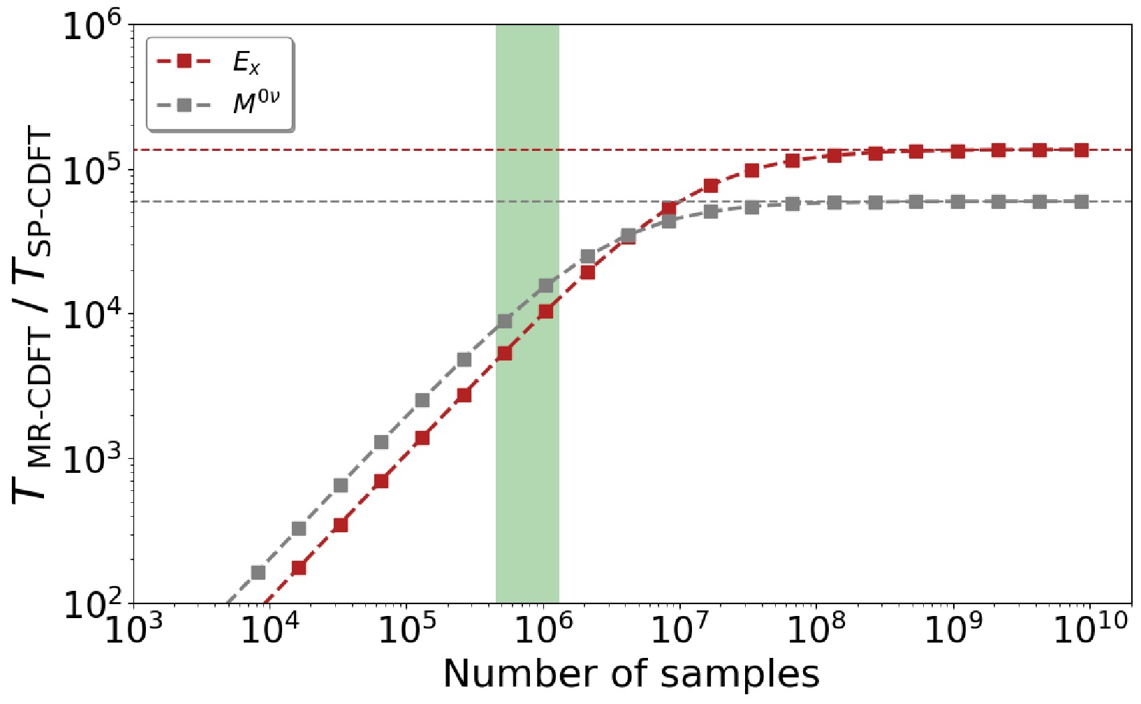
Figure 1. (color online) Speed-up factor of SP-CDFT calculations for nuclear low-lying states and for the NME
$ M^{0\nu} $ of$ 0\nu\beta\beta $ decay in 150Nd. The shaded area indicates the typical sample size.Next, we examine the convergence of the SP-CDFT calculation for the low-lying states
$ 0^+_1 $ ,$ 2^+_1 $ , and$ 4^+_1 $ with respect to the dimension$ N_{\rm EC} $ of configurations, in comparison with the results from MR-CDFT. In the MR-CDFT, we find that the collective wave functions of the$ 0^+_1 $ ,$ 2^+_1 $ , and$ 4^+_1 $ states are mainly concentrated in the region with$ \beta_{20}\in(0.2, 0.4) $ for$ ^{150} {\rm{Nd}}$ , whereas they extend from$ \beta_{20}=-0.2 $ to$ 0.4 $ for$ ^{150} {\rm{Sm}}$ . For the spherical or weakly deformed$ ^{136} {\rm{Xe}}$ and$ ^{136} {\rm{Ba}}$ , they are distributed in the range$ \beta_{20}\in(-0.2, 0.2) $ . Thus, we chose the configurations with quadrupole deformation parameters within the corresponding ranges in the MR-CDFT calculations to generate the basis functions for SP-CDFT. The redundancy in the MR-CDFT calculation is monitored throughout the calculation. We find that, generally, with the choice of step size$ \Delta \beta_2=0.1 $ and cutoff value$ 5\times 10^{-3} $ , the redundancy can be reasonably removed for the states of interest.It is worth pointing out that SP-CDFT is a general configuration-interaction method in which the choice of basis functions can in principle be made arbitrarily as long as the basis is complete. A better choice of basis functions, which are closer to the exact wave function, can significantly reduce the number of required basis functions. In the present work, we focus on the lowest low-lying states, namely
$ 0^+_1 $ ,$ 2^+_1 $ , and$ 4^+_1 $ , in the four isotopes. These states in SP-CDFT are expanded in terms of the wave functions of$ N_{\rm EC} $ states from the MR-CDFT calculations with the same spin and parity. Since the wave functions of these three lowest spin states are not expected to change dramatically with variations of the EDF parameters, they should generally be dominated by the wave functions of the corresponding lowest states obtained from the$ N_t $ training samples, as confirmed in our study. The remaining residual components are expected to be further captured by including the wave functions of excited states with$ \nu\neq 1 $ in the basis. In short, as long as the basis dimension$ N_{\rm EC} $ of SP-CDFT is sufficiently large, one can achieve a rather accurate description of the$ 0^+_1 $ ,$ 2^+_1 $ , and$ 4^+_1 $ states, regardless of whether each basis function itself is an exact MR-CDFT solution.Based on the above idea, we examine the accuracy of SP-CDFT(
$ N_t, k_{\rm max} $ ) as a function of$ N_t $ and$ k_{\rm max} $ . As demonstrated in Ref. [60], choosing$ k_{\rm max} \geq 3 $ effectively reproduces the excitation energy of the$ 2^+_1 $ state. Figure 2 further shows the relative error in the ground-state energy of 150Nd from SP-CDFT($ N_t, k_{\rm max}=3 $ ) calculations across 64 testing sets. Similar behavior is found for the$ 2^+_1 $ and$ 4^+_1 $ states. We note that both the training and testing sets are sampled using the Latin hypercube sampling method [85], which is commonly used to generate representative samples of parameter values from a multidimensional distribution [36, 86−88]. Here, a uniform distribution is chosen as the probability distribution. Following Refs. [78, 79], the parameter ranges for Latin hypercube sampling are selected based on the uncorrelated tolerance of parameters with$ \chi^2 \leqslant \chi^2_{\rm min} + 1 $ . As shown in Fig. 2, as$ N_t $ increases to 14, the mean relative error decreases to 0.04% and stabilizes. Consequently, we select$ N_t = 14 $ for the subsequent calculations.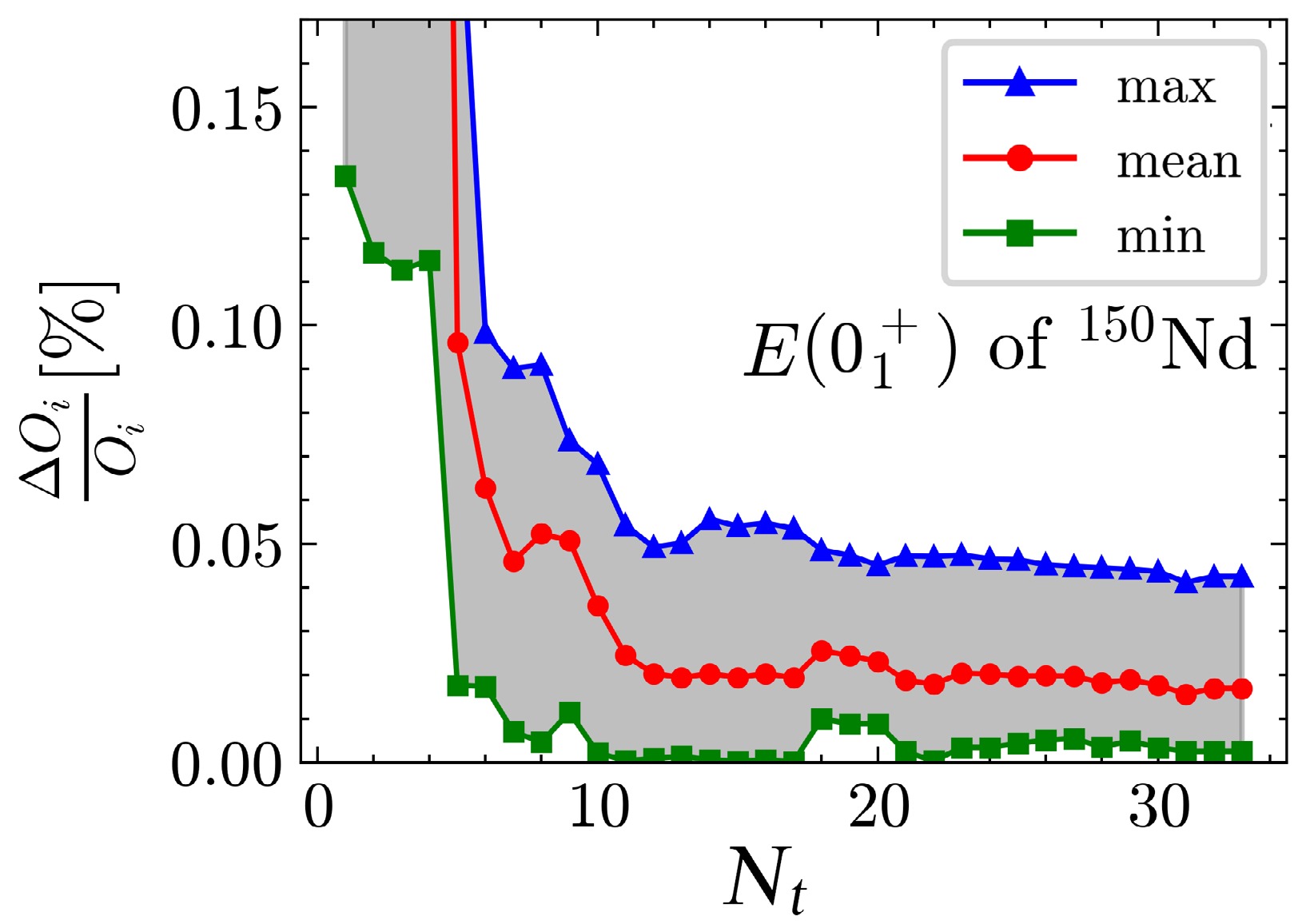
Figure 2. (color online) The minimum, maximum, and mean values of the relative errors in the ground-state energy of
$ ^{150} {\rm{Nd}}$ from the SP-CDFT($ N_t, 3 $ ) calculations for the 64 test sets as a function of the number$ N_t $ of training sets.Figure 3 compares the ground-state energies, root-mean-square (rms) proton radii, excitation energies
$ E_x(2^+_1) $ , and$ B(E2: 0^+_1 \to 2^+_1) $ values obtained from SP-CDFT (14, 3) and MR-CDFT calculations for 150Nd using 64 test sets. The data points align along the diagonal line, indicating strong agreement between the two methods. To quantify the accuracy of the emulator, the standard deviation of the SP-CDFT calculation compared to MR-CDFT is used: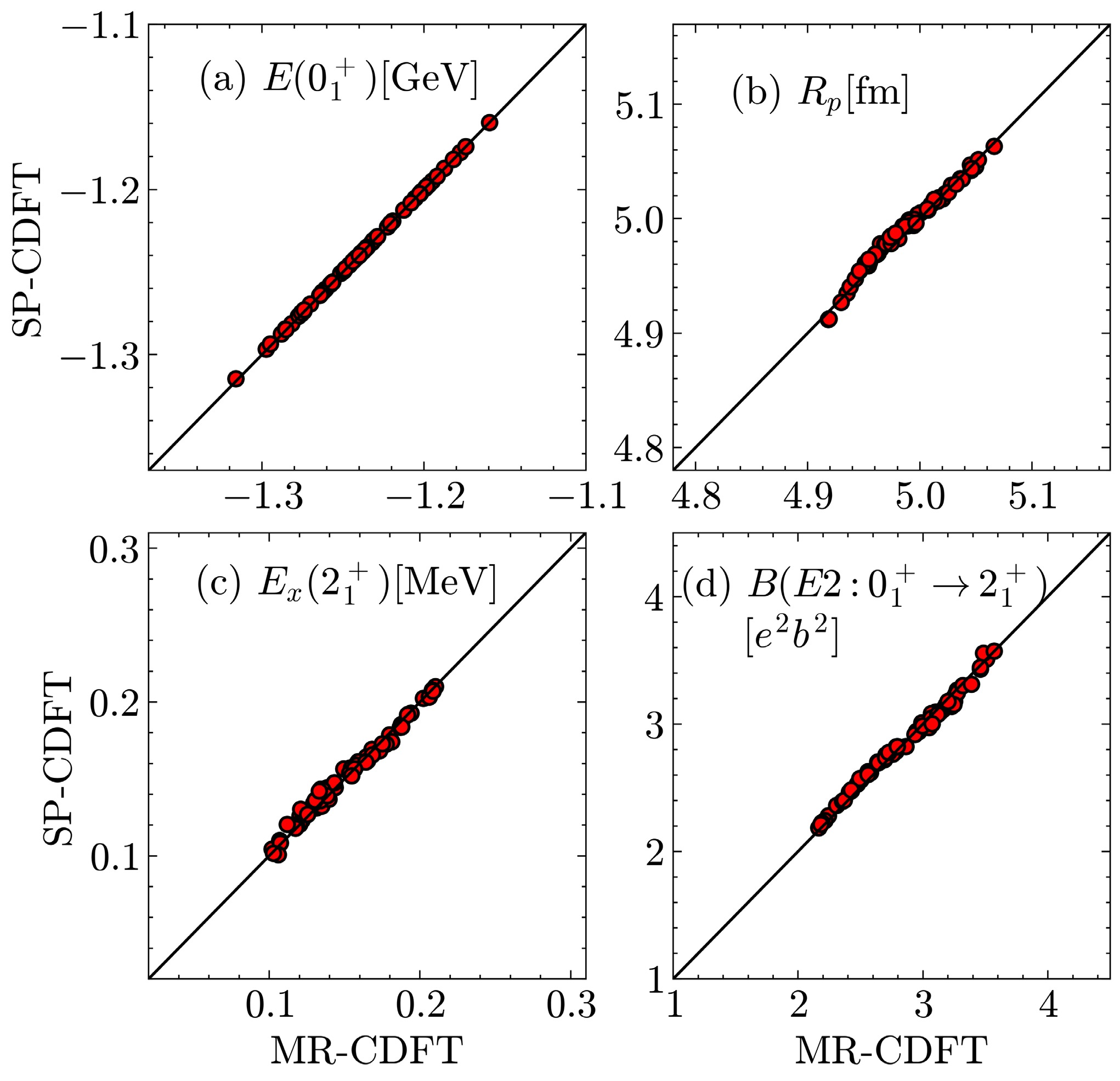
Figure 3. (color online) Comparison of ground-state and low-lying-state properties from SP-CDFT(14,3) and MR-CDFT calculations for 150Nd based on 64 test EDFs.
$ \sigma[O] =\sqrt{\dfrac{1}{N_i}\sum\limits_{i=1}^{N_i} \Bigg(O^{\rm SP-CDFT}_i - O^{\rm MR-CDFT}_i \Bigg)^2}. $
(30) Table 1 presents the standard deviations and their relative values for these four quantities in 150Nd and 150Sm. The ground-state energy
$ E(0^+_1) $ and the proton radius$ R_p $ are reproduced with relative errors of 0.02% and 0.2%, respectively. However, the emulator error for the excitation energy$ E_x(2^+_1) $ , which is several orders of magnitude smaller than the binding energy, is relatively larger, with a relative error of 13%. The relative deviation for$ E_x(2_1^+) $ in 150Sm exceeds that in 150Nd. This can be understood from the fact that the low-lying states of 150Nd exhibit a rather stable prolate deformation with$ \beta_2\simeq0.3 $ , whereas those of 150Sm involve admixtures of weakly deformed configurations and display a more extended distribution of collective wave functions [84]. Consequently, their representation with the same number of basis functions as used for 150Nd is less accurate. The$ E2 $ transition strengths are reproduced with greater accuracy. We also checked the relative errors of the SP-CDFT calculations for 136Xe and 136Ba, finding them to be generally less than 6%.Nuclei $ E(0^+_1) $ /MeV$ R_p $ /fm$ E_x(2^+_1) $ /MeV$ B(E2) $ ($ e^2 $ b$ ^2 $ )σ $ \cal{R} $ [%]σ $ \cal{R} $ [%]σ $ \cal{R} $ σ $ \cal{R} $ [%]$ ^{150} {\rm{Nd}}$ 0.272 0.02 0.003 0.2 0.006 4 0.063 2 $ ^{150} {\rm{Sm}}$ 0.180 0.01 0.005 0.1 0.040 13 0.071 4 Table 1. The standard deviations
$ \sigma(O) $ and relative deviations$ {\cal{R}}(O)=\sigma(O)/O^{\rm MR-CDFT} $ of the SP-CDFT calculations relative to the MR-CDFT results are presented, based on 64 parameter sets of EDFs. Results are shown for the ground-state energy$ E(0^+_1) $ , proton radius$ R_p $ , excitation energy$ E_x(2^+_1) $ , and transition probability$ B(E2: 0^+_1 \to 2^+_1) $ of 150Nd and 150Sm.We note that increasing the number of benchmark points would improve the statistical precision of the deviations reported in Table 1, but it is not expected to affect the main conclusions of the subsequent statistical analysis. The 64 test parametrizations already provide a space-filling sample of the relevant parameter domain, and the observed SP-CDFT deviations from MR-CDFT are small compared with the propagated statistical uncertainties. Moreover, since the final probability distributions are obtained from ensemble averages over millions of EDF samples, residual sample-by-sample emulation errors are expected to be largely averaged out.
-
The time complexity of MR-CDFT calculations for
$ N_{{\boldsymbol{C}}_\odot} $ target parameter sets is given by$ T_{\rm MR-CDFT} =O\Big(N^2_{{\boldsymbol{q}} }N_{{\boldsymbol{C}}_\odot}\Big)\Delta T_1, $
(28) where
$ \Delta T_1 $ represents the computational time for each GCM kernel. In contrast, the time complexity of the SP-CDFT($ N_t $ ,$ k_{\rm max} $ ) comprises$ T_{\rm SP-CDFT} = O\Big( N^2_{{\boldsymbol{q}} } N^2_t \Big)\Delta T_1 + O\Big(N^2_{\rm EC}N_{{\boldsymbol{C}}_\odot}\Big)\Delta T_2. $
(29) where the first term represents the computational time of
$ N_t $ training sets, while the second term represents the time needed to evaluate the EC kernels of$ N_{{\boldsymbol{C}}_\odot} $ target sets, with$ N_{\rm EC}=N_tk_{\rm max} $ . It is seen that$ T_{\rm SP-CDFT}>T_{\rm MR-CDFT} $ for$ N_{{\boldsymbol{C}}_\odot}<N^2_t $ . As$ N_{{\boldsymbol{C}}_\odot} $ increases, both$ T_{\rm MR-CDFT} $ and$ T_{\rm SP-CDFT} $ increase linearly, but with slopes of$ N^2_{{\boldsymbol{q}} }\Delta T_1 $ and$ N^2_{\rm EC}\Delta T_2 $ , respectively. By decomposing the interaction energy (4) into nine terms, one can compute the Hamiltonian kernels of EC efficiently using the GCM kernels of the training EDFs; see Eq. (25). Quantitatively, we find$ \Delta T_1/\Delta T_2\simeq 10^5 $ for 150Nd. In other words, one would expect$ T_{\rm SP-CDFT}\ll T_{\rm MR-CDFT} $ when the number of target sets$ N_{{\boldsymbol{C}}_\odot} $ is sufficiently large.Figure 1 displays the speed-up factor, defined as the ratio of
$ T_{\rm MR-CDFT} $ to$ T_{\rm SP-CDFT} $ for nuclear low-lying states and the NME$ M^{0\nu} $ of$ 0\nu\beta\beta $ decay, as a function of$ N_{{\boldsymbol{C}}_\odot} $ . The$ M^{0\nu} $ is computed using the transition operators based on the standard mechanism; see Refs. [52, 84] for details. Since$ T_{\rm MR-CDFT} $ increases linearly with the number of samples, whereas$ T_{\rm SP-CDFT} $ barely changes with it, the speed-up factor$ T_{\rm MR-CDFT}/T_{\rm SP-CDFT} $ increases almost linearly up to$ 10^4 $ when the number of sampling EDFs reaches$ 10^6 $ . It is also seen from Fig. 1 that the speed-up factor asymptotically approaches a limit as the number of samples increases up to$ 10^8 $ , i.e.,$ T_{\rm MR-CDFT}/T_{\rm SP-CDFT}\to (N_{{\boldsymbol{q}} }/N_{\rm EC})^2 (\Delta T_1/\Delta T_2) $ . A similar behavior has been found in Ref. [68]. In short, SP-CDFT enables the prediction of nuclear low-lying states for millions of EDF parameter sets within half an hour on a personal computer, whereas the corresponding MR-CDFT calculations would otherwise require years on a typical CPU platform, such as an Intel Xeon 8488C 2.4 GHz processor with 48 cores.
Figure 1. (color online) Speed-up factor of SP-CDFT calculations for nuclear low-lying states and for the NME
$ M^{0\nu} $ of$ 0\nu\beta\beta $ decay in 150Nd. The shaded area indicates the typical sample size.Next, we examine the convergence of the SP-CDFT calculation for the low-lying states
$ 0^+_1 $ ,$ 2^+_1 $ , and$ 4^+_1 $ with respect to the dimension$ N_{\rm EC} $ of configurations, in comparison with the results from MR-CDFT. In the MR-CDFT, we find that the collective wave functions of the$ 0^+_1 $ ,$ 2^+_1 $ , and$ 4^+_1 $ states are mainly concentrated in the region with$ \beta_{20}\in(0.2, 0.4) $ for$ ^{150} {\rm{Nd}}$ , whereas they extend from$ \beta_{20}=-0.2 $ to$ 0.4 $ for$ ^{150} {\rm{Sm}}$ . For the spherical or weakly deformed$ ^{136} {\rm{Xe}}$ and$ ^{136} {\rm{Ba}}$ , they are distributed in the range$ \beta_{20}\in(-0.2, 0.2) $ . Thus, we chose the configurations with quadrupole deformation parameters within the corresponding ranges in the MR-CDFT calculations to generate the basis functions for SP-CDFT. The redundancy in the MR-CDFT calculation is monitored throughout the calculation. We find that, generally, with the choice of step size$ \Delta \beta_2=0.1 $ and cutoff value$ 5\times 10^{-3} $ , the redundancy can be reasonably removed for the states of interest.It is worth pointing out that SP-CDFT is a general configuration-interaction method in which the choice of basis functions can in principle be made arbitrarily as long as the basis is complete. A better choice of basis functions, which are closer to the exact wave function, can significantly reduce the number of required basis functions. In the present work, we focus on the lowest low-lying states, namely
$ 0^+_1 $ ,$ 2^+_1 $ , and$ 4^+_1 $ , in the four isotopes. These states in SP-CDFT are expanded in terms of the wave functions of$ N_{\rm EC} $ states from the MR-CDFT calculations with the same spin and parity. Since the wave functions of these three lowest spin states are not expected to change dramatically with variations of the EDF parameters, they should generally be dominated by the wave functions of the corresponding lowest states obtained from the$ N_t $ training samples, as confirmed in our study. The remaining residual components are expected to be further captured by including the wave functions of excited states with$ \nu\neq 1 $ in the basis. In short, as long as the basis dimension$ N_{\rm EC} $ of SP-CDFT is sufficiently large, one can achieve a rather accurate description of the$ 0^+_1 $ ,$ 2^+_1 $ , and$ 4^+_1 $ states, regardless of whether each basis function itself is an exact MR-CDFT solution.Based on the above idea, we examine the accuracy of SP-CDFT(
$ N_t, k_{\rm max} $ ) as a function of$ N_t $ and$ k_{\rm max} $ . As demonstrated in Ref. [60], choosing$ k_{\rm max} \geq 3 $ effectively reproduces the excitation energy of the$ 2^+_1 $ state. Figure 2 further shows the relative error in the ground-state energy of 150Nd from SP-CDFT($ N_t, k_{\rm max}=3 $ ) calculations across 64 testing sets. Similar behavior is found for the$ 2^+_1 $ and$ 4^+_1 $ states. We note that both the training and testing sets are sampled using the Latin hypercube sampling method [85], which is commonly used to generate representative samples of parameter values from a multidimensional distribution [36, 86−88]. Here, a uniform distribution is chosen as the probability distribution. Following Refs. [78, 79], the parameter ranges for Latin hypercube sampling are selected based on the uncorrelated tolerance of parameters with$ \chi^2 \leqslant \chi^2_{\rm min} + 1 $ . As shown in Fig. 2, as$ N_t $ increases to 14, the mean relative error decreases to 0.04% and stabilizes. Consequently, we select$ N_t = 14 $ for the subsequent calculations.
Figure 2. (color online) The minimum, maximum, and mean values of the relative errors in the ground-state energy of
$ ^{150} {\rm{Nd}}$ from the SP-CDFT($ N_t, 3 $ ) calculations for the 64 test sets as a function of the number$ N_t $ of training sets.Figure 3 compares the ground-state energies, root-mean-square (rms) proton radii, excitation energies
$ E_x(2^+_1) $ , and$ B(E2: 0^+_1 \to 2^+_1) $ values obtained from SP-CDFT (14, 3) and MR-CDFT calculations for 150Nd using 64 test sets. The data points align along the diagonal line, indicating strong agreement between the two methods. To quantify the accuracy of the emulator, the standard deviation of the SP-CDFT calculation compared to MR-CDFT is used:
Figure 3. (color online) Comparison of ground-state and low-lying-state properties from SP-CDFT(14,3) and MR-CDFT calculations for 150Nd based on 64 test EDFs.
$ \sigma[O] =\sqrt{\dfrac{1}{N_i}\sum\limits_{i=1}^{N_i} \Bigg(O^{\rm SP-CDFT}_i - O^{\rm MR-CDFT}_i \Bigg)^2}. $
(30) Table 1 presents the standard deviations and their relative values for these four quantities in 150Nd and 150Sm. The ground-state energy
$ E(0^+_1) $ and the proton radius$ R_p $ are reproduced with relative errors of 0.02% and 0.2%, respectively. However, the emulator error for the excitation energy$ E_x(2^+_1) $ , which is several orders of magnitude smaller than the binding energy, is relatively larger, with a relative error of 13%. The relative deviation for$ E_x(2_1^+) $ in 150Sm exceeds that in 150Nd. This can be understood from the fact that the low-lying states of 150Nd exhibit a rather stable prolate deformation with$ \beta_2\simeq0.3 $ , whereas those of 150Sm involve admixtures of weakly deformed configurations and display a more extended distribution of collective wave functions [84]. Consequently, their representation with the same number of basis functions as used for 150Nd is less accurate. The$ E2 $ transition strengths are reproduced with greater accuracy. We also checked the relative errors of the SP-CDFT calculations for 136Xe and 136Ba, finding them to be generally less than 6%.Nuclei $ E(0^+_1) $ /MeV$ R_p $ /fm$ E_x(2^+_1) $ /MeV$ B(E2) $ ($ e^2 $ b$ ^2 $ )σ $ \cal{R} $ [%]σ $ \cal{R} $ [%]σ $ \cal{R} $ σ $ \cal{R} $ [%]$ ^{150} {\rm{Nd}}$ 0.272 0.02 0.003 0.2 0.006 4 0.063 2 $ ^{150} {\rm{Sm}}$ 0.180 0.01 0.005 0.1 0.040 13 0.071 4 Table 1. The standard deviations
$ \sigma(O) $ and relative deviations$ {\cal{R}}(O)=\sigma(O)/O^{\rm MR-CDFT} $ of the SP-CDFT calculations relative to the MR-CDFT results are presented, based on 64 parameter sets of EDFs. Results are shown for the ground-state energy$ E(0^+_1) $ , proton radius$ R_p $ , excitation energy$ E_x(2^+_1) $ , and transition probability$ B(E2: 0^+_1 \to 2^+_1) $ of 150Nd and 150Sm.We note that increasing the number of benchmark points would improve the statistical precision of the deviations reported in Table 1, but it is not expected to affect the main conclusions of the subsequent statistical analysis. The 64 test parametrizations already provide a space-filling sample of the relevant parameter domain, and the observed SP-CDFT deviations from MR-CDFT are small compared with the propagated statistical uncertainties. Moreover, since the final probability distributions are obtained from ensemble averages over millions of EDF samples, residual sample-by-sample emulation errors are expected to be largely averaged out.
-
The time complexity of MR-CDFT calculations for
$ N_{{\boldsymbol{C}}_\odot} $ target parameter sets is given by$ T_{\rm MR-CDFT} =O\Big(N^2_{{\boldsymbol{q}} }N_{{\boldsymbol{C}}_\odot}\Big)\Delta T_1, $
(28) where
$ \Delta T_1 $ represents the computational time for each GCM kernel. In contrast, the time complexity of the SP-CDFT($ N_t $ ,$ k_{\rm max} $ ) comprises$ T_{\rm SP-CDFT} = O\Big( N^2_{{\boldsymbol{q}} } N^2_t \Big)\Delta T_1 + O\Big(N^2_{\rm EC}N_{{\boldsymbol{C}}_\odot}\Big)\Delta T_2. $
(29) where the first term represents the computational time of
$ N_t $ training sets, while the second term represents the time needed to evaluate the EC kernels of$ N_{{\boldsymbol{C}}_\odot} $ target sets, with$ N_{\rm EC}=N_tk_{\rm max} $ . It is seen that$ T_{\rm SP-CDFT}>T_{\rm MR-CDFT} $ for$ N_{{\boldsymbol{C}}_\odot}<N^2_t $ . As$ N_{{\boldsymbol{C}}_\odot} $ increases, both$ T_{\rm MR-CDFT} $ and$ T_{\rm SP-CDFT} $ increase linearly, but with slopes of$ N^2_{{\boldsymbol{q}} }\Delta T_1 $ and$ N^2_{\rm EC}\Delta T_2 $ , respectively. By decomposing the interaction energy (4) into nine terms, one can compute the Hamiltonian kernels of EC efficiently using the GCM kernels of the training EDFs; see Eq. (25). Quantitatively, we find$ \Delta T_1/\Delta T_2\simeq 10^5 $ for 150Nd. In other words, one would expect$ T_{\rm SP-CDFT}\ll T_{\rm MR-CDFT} $ when the number of target sets$ N_{{\boldsymbol{C}}_\odot} $ is sufficiently large.Figure 1 displays the speed-up factor, defined as the ratio of
$ T_{\rm MR-CDFT} $ to$ T_{\rm SP-CDFT} $ for nuclear low-lying states and the NME$ M^{0\nu} $ of$ 0\nu\beta\beta $ decay, as a function of$ N_{{\boldsymbol{C}}_\odot} $ . The$ M^{0\nu} $ is computed using the transition operators based on the standard mechanism; see Refs. [52, 84] for details. Since$ T_{\rm MR-CDFT} $ increases linearly with the number of samples, whereas$ T_{\rm SP-CDFT} $ barely changes with it, the speed-up factor$ T_{\rm MR-CDFT}/T_{\rm SP-CDFT} $ increases almost linearly up to$ 10^4 $ when the number of sampling EDFs reaches$ 10^6 $ . It is also seen from Fig. 1 that the speed-up factor asymptotically approaches a limit as the number of samples increases up to$ 10^8 $ , i.e.,$ T_{\rm MR-CDFT}/T_{\rm SP-CDFT}\to (N_{{\boldsymbol{q}} }/N_{\rm EC})^2 (\Delta T_1/\Delta T_2) $ . A similar behavior has been found in Ref. [68]. In short, SP-CDFT enables the prediction of nuclear low-lying states for millions of EDF parameter sets within half an hour on a personal computer, whereas the corresponding MR-CDFT calculations would otherwise require years on a typical CPU platform, such as an Intel Xeon 8488C 2.4 GHz processor with 48 cores.
Figure 1. (color online) Speed-up factor of SP-CDFT calculations for nuclear low-lying states and for the NME
$ M^{0\nu} $ of$ 0\nu\beta\beta $ decay in 150Nd. The shaded area indicates the typical sample size.Next, we examine the convergence of the SP-CDFT calculation for the low-lying states
$ 0^+_1 $ ,$ 2^+_1 $ , and$ 4^+_1 $ with respect to the dimension$ N_{\rm EC} $ of configurations, in comparison with the results from MR-CDFT. In the MR-CDFT, we find that the collective wave functions of the$ 0^+_1 $ ,$ 2^+_1 $ , and$ 4^+_1 $ states are mainly concentrated in the region with$ \beta_{20}\in(0.2, 0.4) $ for$ ^{150} {\rm{Nd}}$ , whereas they extend from$ \beta_{20}=-0.2 $ to$ 0.4 $ for$ ^{150} {\rm{Sm}}$ . For the spherical or weakly deformed$ ^{136} {\rm{Xe}}$ and$ ^{136} {\rm{Ba}}$ , they are distributed in the range$ \beta_{20}\in(-0.2, 0.2) $ . Thus, we chose the configurations with quadrupole deformation parameters within the corresponding ranges in the MR-CDFT calculations to generate the basis functions for SP-CDFT. The redundancy in the MR-CDFT calculation is monitored throughout the calculation. We find that, generally, with the choice of step size$ \Delta \beta_2=0.1 $ and cutoff value$ 5\times 10^{-3} $ , the redundancy can be reasonably removed for the states of interest.It is worth pointing out that SP-CDFT is a general configuration-interaction method in which the choice of basis functions can in principle be made arbitrarily as long as the basis is complete. A better choice of basis functions, which are closer to the exact wave function, can significantly reduce the number of required basis functions. In the present work, we focus on the lowest low-lying states, namely
$ 0^+_1 $ ,$ 2^+_1 $ , and$ 4^+_1 $ , in the four isotopes. These states in SP-CDFT are expanded in terms of the wave functions of$ N_{\rm EC} $ states from the MR-CDFT calculations with the same spin and parity. Since the wave functions of these three lowest spin states are not expected to change dramatically with variations of the EDF parameters, they should generally be dominated by the wave functions of the corresponding lowest states obtained from the$ N_t $ training samples, as confirmed in our study. The remaining residual components are expected to be further captured by including the wave functions of excited states with$ \nu\neq 1 $ in the basis. In short, as long as the basis dimension$ N_{\rm EC} $ of SP-CDFT is sufficiently large, one can achieve a rather accurate description of the$ 0^+_1 $ ,$ 2^+_1 $ , and$ 4^+_1 $ states, regardless of whether each basis function itself is an exact MR-CDFT solution.Based on the above idea, we examine the accuracy of SP-CDFT(
$ N_t, k_{\rm max} $ ) as a function of$ N_t $ and$ k_{\rm max} $ . As demonstrated in Ref. [60], choosing$ k_{\rm max} \geq 3 $ effectively reproduces the excitation energy of the$ 2^+_1 $ state. Figure 2 further shows the relative error in the ground-state energy of 150Nd from SP-CDFT($ N_t, k_{\rm max}=3 $ ) calculations across 64 testing sets. Similar behavior is found for the$ 2^+_1 $ and$ 4^+_1 $ states. We note that both the training and testing sets are sampled using the Latin hypercube sampling method [85], which is commonly used to generate representative samples of parameter values from a multidimensional distribution [36, 86−88]. Here, a uniform distribution is chosen as the probability distribution. Following Refs. [78, 79], the parameter ranges for Latin hypercube sampling are selected based on the uncorrelated tolerance of parameters with$ \chi^2 \leqslant \chi^2_{\rm min} + 1 $ . As shown in Fig. 2, as$ N_t $ increases to 14, the mean relative error decreases to 0.04% and stabilizes. Consequently, we select$ N_t = 14 $ for the subsequent calculations.
Figure 2. (color online) The minimum, maximum, and mean values of the relative errors in the ground-state energy of
$ ^{150} {\rm{Nd}}$ from the SP-CDFT($ N_t, 3 $ ) calculations for the 64 test sets as a function of the number$ N_t $ of training sets.Figure 3 compares the ground-state energies, root-mean-square (rms) proton radii, excitation energies
$ E_x(2^+_1) $ , and$ B(E2: 0^+_1 \to 2^+_1) $ values obtained from SP-CDFT (14, 3) and MR-CDFT calculations for 150Nd using 64 test sets. The data points align along the diagonal line, indicating strong agreement between the two methods. To quantify the accuracy of the emulator, the standard deviation of the SP-CDFT calculation compared to MR-CDFT is used:
Figure 3. (color online) Comparison of ground-state and low-lying-state properties from SP-CDFT(14,3) and MR-CDFT calculations for 150Nd based on 64 test EDFs.
$ \sigma[O] =\sqrt{\dfrac{1}{N_i}\sum\limits_{i=1}^{N_i} \Bigg(O^{\rm SP-CDFT}_i - O^{\rm MR-CDFT}_i \Bigg)^2}. $
(30) Table 1 presents the standard deviations and their relative values for these four quantities in 150Nd and 150Sm. The ground-state energy
$ E(0^+_1) $ and the proton radius$ R_p $ are reproduced with relative errors of 0.02% and 0.2%, respectively. However, the emulator error for the excitation energy$ E_x(2^+_1) $ , which is several orders of magnitude smaller than the binding energy, is relatively larger, with a relative error of 13%. The relative deviation for$ E_x(2_1^+) $ in 150Sm exceeds that in 150Nd. This can be understood from the fact that the low-lying states of 150Nd exhibit a rather stable prolate deformation with$ \beta_2\simeq0.3 $ , whereas those of 150Sm involve admixtures of weakly deformed configurations and display a more extended distribution of collective wave functions [84]. Consequently, their representation with the same number of basis functions as used for 150Nd is less accurate. The$ E2 $ transition strengths are reproduced with greater accuracy. We also checked the relative errors of the SP-CDFT calculations for 136Xe and 136Ba, finding them to be generally less than 6%.Nuclei $ E(0^+_1) $ /MeV$ R_p $ /fm$ E_x(2^+_1) $ /MeV$ B(E2) $ ($ e^2 $ b$ ^2 $ )σ $ \cal{R} $ [%]σ $ \cal{R} $ [%]σ $ \cal{R} $ σ $ \cal{R} $ [%]$ ^{150} {\rm{Nd}}$ 0.272 0.02 0.003 0.2 0.006 4 0.063 2 $ ^{150} {\rm{Sm}}$ 0.180 0.01 0.005 0.1 0.040 13 0.071 4 Table 1. The standard deviations
$ \sigma(O) $ and relative deviations$ {\cal{R}}(O)=\sigma(O)/O^{\rm MR-CDFT} $ of the SP-CDFT calculations relative to the MR-CDFT results are presented, based on 64 parameter sets of EDFs. Results are shown for the ground-state energy$ E(0^+_1) $ , proton radius$ R_p $ , excitation energy$ E_x(2^+_1) $ , and transition probability$ B(E2: 0^+_1 \to 2^+_1) $ of 150Nd and 150Sm.We note that increasing the number of benchmark points would improve the statistical precision of the deviations reported in Table 1, but it is not expected to affect the main conclusions of the subsequent statistical analysis. The 64 test parametrizations already provide a space-filling sample of the relevant parameter domain, and the observed SP-CDFT deviations from MR-CDFT are small compared with the propagated statistical uncertainties. Moreover, since the final probability distributions are obtained from ensemble averages over millions of EDF samples, residual sample-by-sample emulation errors are expected to be largely averaged out.
-
The time complexity of MR-CDFT calculations for
$ N_{{\boldsymbol{C}}_\odot} $ target parameter sets is given by$ T_{\rm MR-CDFT} =O\Big(N^2_{{\boldsymbol{q}} }N_{{\boldsymbol{C}}_\odot}\Big)\Delta T_1, $
(28) where
$ \Delta T_1 $ represents the computational time for each GCM kernel. In contrast, the time complexity of the SP-CDFT($ N_t $ ,$ k_{\rm max} $ ) comprises$ T_{\rm SP-CDFT} = O\Big( N^2_{{\boldsymbol{q}} } N^2_t \Big)\Delta T_1 + O\Big(N^2_{\rm EC}N_{{\boldsymbol{C}}_\odot}\Big)\Delta T_2. $
(29) where the first term represents the computational time of
$ N_t $ training sets, while the second term represents the time needed to evaluate the EC kernels of$ N_{{\boldsymbol{C}}_\odot} $ target sets, with$ N_{\rm EC}=N_tk_{\rm max} $ . It is seen that$ T_{\rm SP-CDFT}>T_{\rm MR-CDFT} $ for$ N_{{\boldsymbol{C}}_\odot}<N^2_t $ . As$ N_{{\boldsymbol{C}}_\odot} $ increases, both$ T_{\rm MR-CDFT} $ and$ T_{\rm SP-CDFT} $ increase linearly, but with slopes of$ N^2_{{\boldsymbol{q}} }\Delta T_1 $ and$ N^2_{\rm EC}\Delta T_2 $ , respectively. By decomposing the interaction energy (4) into nine terms, one can compute the Hamiltonian kernels of EC efficiently using the GCM kernels of the training EDFs; see Eq. (25). Quantitatively, we find$ \Delta T_1/\Delta T_2\simeq 10^5 $ for 150Nd. In other words, one would expect$ T_{\rm SP-CDFT}\ll T_{\rm MR-CDFT} $ when the number of target sets$ N_{{\boldsymbol{C}}_\odot} $ is sufficiently large.Figure 1 displays the speed-up factor, defined as the ratio of
$ T_{\rm MR-CDFT} $ to$ T_{\rm SP-CDFT} $ for nuclear low-lying states and the NME$ M^{0\nu} $ of$ 0\nu\beta\beta $ decay, as a function of$ N_{{\boldsymbol{C}}_\odot} $ . The$ M^{0\nu} $ is computed using the transition operators based on the standard mechanism; see Refs. [52, 84] for details. Since$ T_{\rm MR-CDFT} $ increases linearly with the number of samples, whereas$ T_{\rm SP-CDFT} $ barely changes with it, the speed-up factor$ T_{\rm MR-CDFT}/T_{\rm SP-CDFT} $ increases almost linearly up to$ 10^4 $ when the number of sampling EDFs reaches$ 10^6 $ . It is also seen from Fig. 1 that the speed-up factor asymptotically approaches a limit as the number of samples increases up to$ 10^8 $ , i.e.,$ T_{\rm MR-CDFT}/T_{\rm SP-CDFT}\to (N_{{\boldsymbol{q}} }/N_{\rm EC})^2 (\Delta T_1/\Delta T_2) $ . A similar behavior has been found in Ref. [68]. In short, SP-CDFT enables the prediction of nuclear low-lying states for millions of EDF parameter sets within half an hour on a personal computer, whereas the corresponding MR-CDFT calculations would otherwise require years on a typical CPU platform, such as an Intel Xeon 8488C 2.4 GHz processor with 48 cores.
Figure 1. (color online) Speed-up factor of SP-CDFT calculations for nuclear low-lying states and for the NME
$ M^{0\nu} $ of$ 0\nu\beta\beta $ decay in 150Nd. The shaded area indicates the typical sample size.Next, we examine the convergence of the SP-CDFT calculation for the low-lying states
$ 0^+_1 $ ,$ 2^+_1 $ , and$ 4^+_1 $ with respect to the dimension$ N_{\rm EC} $ of configurations, in comparison with the results from MR-CDFT. In the MR-CDFT, we find that the collective wave functions of the$ 0^+_1 $ ,$ 2^+_1 $ , and$ 4^+_1 $ states are mainly concentrated in the region with$ \beta_{20}\in(0.2, 0.4) $ for$ ^{150} {\rm{Nd}}$ , whereas they extend from$ \beta_{20}=-0.2 $ to$ 0.4 $ for$ ^{150} {\rm{Sm}}$ . For the spherical or weakly deformed$ ^{136} {\rm{Xe}}$ and$ ^{136} {\rm{Ba}}$ , they are distributed in the range$ \beta_{20}\in(-0.2, 0.2) $ . Thus, we chose the configurations with quadrupole deformation parameters within the corresponding ranges in the MR-CDFT calculations to generate the basis functions for SP-CDFT. The redundancy in the MR-CDFT calculation is monitored throughout the calculation. We find that, generally, with the choice of step size$ \Delta \beta_2=0.1 $ and cutoff value$ 5\times 10^{-3} $ , the redundancy can be reasonably removed for the states of interest.It is worth pointing out that SP-CDFT is a general configuration-interaction method in which the choice of basis functions can in principle be made arbitrarily as long as the basis is complete. A better choice of basis functions, which are closer to the exact wave function, can significantly reduce the number of required basis functions. In the present work, we focus on the lowest low-lying states, namely
$ 0^+_1 $ ,$ 2^+_1 $ , and$ 4^+_1 $ , in the four isotopes. These states in SP-CDFT are expanded in terms of the wave functions of$ N_{\rm EC} $ states from the MR-CDFT calculations with the same spin and parity. Since the wave functions of these three lowest spin states are not expected to change dramatically with variations of the EDF parameters, they should generally be dominated by the wave functions of the corresponding lowest states obtained from the$ N_t $ training samples, as confirmed in our study. The remaining residual components are expected to be further captured by including the wave functions of excited states with$ \nu\neq 1 $ in the basis. In short, as long as the basis dimension$ N_{\rm EC} $ of SP-CDFT is sufficiently large, one can achieve a rather accurate description of the$ 0^+_1 $ ,$ 2^+_1 $ , and$ 4^+_1 $ states, regardless of whether each basis function itself is an exact MR-CDFT solution.Based on the above idea, we examine the accuracy of SP-CDFT(
$ N_t, k_{\rm max} $ ) as a function of$ N_t $ and$ k_{\rm max} $ . As demonstrated in Ref. [60], choosing$ k_{\rm max} \geq 3 $ effectively reproduces the excitation energy of the$ 2^+_1 $ state. Figure 2 further shows the relative error in the ground-state energy of 150Nd from SP-CDFT($ N_t, k_{\rm max}=3 $ ) calculations across 64 testing sets. Similar behavior is found for the$ 2^+_1 $ and$ 4^+_1 $ states. We note that both the training and testing sets are sampled using the Latin hypercube sampling method [85], which is commonly used to generate representative samples of parameter values from a multidimensional distribution [36, 86−88]. Here, a uniform distribution is chosen as the probability distribution. Following Refs. [78, 79], the parameter ranges for Latin hypercube sampling are selected based on the uncorrelated tolerance of parameters with$ \chi^2 \leqslant \chi^2_{\rm min} + 1 $ . As shown in Fig. 2, as$ N_t $ increases to 14, the mean relative error decreases to 0.04% and stabilizes. Consequently, we select$ N_t = 14 $ for the subsequent calculations.
Figure 2. (color online) The minimum, maximum, and mean values of the relative errors in the ground-state energy of
$ ^{150} {\rm{Nd}}$ from the SP-CDFT($ N_t, 3 $ ) calculations for the 64 test sets as a function of the number$ N_t $ of training sets.Figure 3 compares the ground-state energies, root-mean-square (rms) proton radii, excitation energies
$ E_x(2^+_1) $ , and$ B(E2: 0^+_1 \to 2^+_1) $ values obtained from SP-CDFT (14, 3) and MR-CDFT calculations for 150Nd using 64 test sets. The data points align along the diagonal line, indicating strong agreement between the two methods. To quantify the accuracy of the emulator, the standard deviation of the SP-CDFT calculation compared to MR-CDFT is used:
Figure 3. (color online) Comparison of ground-state and low-lying-state properties from SP-CDFT(14,3) and MR-CDFT calculations for 150Nd based on 64 test EDFs.
$ \sigma[O] =\sqrt{\dfrac{1}{N_i}\sum\limits_{i=1}^{N_i} \Bigg(O^{\rm SP-CDFT}_i - O^{\rm MR-CDFT}_i \Bigg)^2}. $
(30) Table 1 presents the standard deviations and their relative values for these four quantities in 150Nd and 150Sm. The ground-state energy
$ E(0^+_1) $ and the proton radius$ R_p $ are reproduced with relative errors of 0.02% and 0.2%, respectively. However, the emulator error for the excitation energy$ E_x(2^+_1) $ , which is several orders of magnitude smaller than the binding energy, is relatively larger, with a relative error of 13%. The relative deviation for$ E_x(2_1^+) $ in 150Sm exceeds that in 150Nd. This can be understood from the fact that the low-lying states of 150Nd exhibit a rather stable prolate deformation with$ \beta_2\simeq0.3 $ , whereas those of 150Sm involve admixtures of weakly deformed configurations and display a more extended distribution of collective wave functions [84]. Consequently, their representation with the same number of basis functions as used for 150Nd is less accurate. The$ E2 $ transition strengths are reproduced with greater accuracy. We also checked the relative errors of the SP-CDFT calculations for 136Xe and 136Ba, finding them to be generally less than 6%.Nuclei $ E(0^+_1) $ /MeV$ R_p $ /fm$ E_x(2^+_1) $ /MeV$ B(E2) $ ($ e^2 $ b$ ^2 $ )σ $ \cal{R} $ [%]σ $ \cal{R} $ [%]σ $ \cal{R} $ σ $ \cal{R} $ [%]$ ^{150} {\rm{Nd}}$ 0.272 0.02 0.003 0.2 0.006 4 0.063 2 $ ^{150} {\rm{Sm}}$ 0.180 0.01 0.005 0.1 0.040 13 0.071 4 Table 1. The standard deviations
$ \sigma(O) $ and relative deviations$ {\cal{R}}(O)=\sigma(O)/O^{\rm MR-CDFT} $ of the SP-CDFT calculations relative to the MR-CDFT results are presented, based on 64 parameter sets of EDFs. Results are shown for the ground-state energy$ E(0^+_1) $ , proton radius$ R_p $ , excitation energy$ E_x(2^+_1) $ , and transition probability$ B(E2: 0^+_1 \to 2^+_1) $ of 150Nd and 150Sm.We note that increasing the number of benchmark points would improve the statistical precision of the deviations reported in Table 1, but it is not expected to affect the main conclusions of the subsequent statistical analysis. The 64 test parametrizations already provide a space-filling sample of the relevant parameter domain, and the observed SP-CDFT deviations from MR-CDFT are small compared with the propagated statistical uncertainties. Moreover, since the final probability distributions are obtained from ensemble averages over millions of EDF samples, residual sample-by-sample emulation errors are expected to be largely averaged out.
-
The single-particle state in infinite nuclear matter is labeled by the momentum
$ {\boldsymbol{p}}=\hbar{\boldsymbol{k}} $ and the spin direction λ. The corresponding single-particle wave function reduces to$ u_\tau({\boldsymbol{k}},\lambda) $ , which satisfies the following Dirac equation:$ \left({\boldsymbol{\alpha}}\cdot{\boldsymbol{k}} + \beta M^*_\tau +\Sigma_{\tau}^{0}\right)u_\tau({\boldsymbol{k}},\lambda) = E_\tau({\boldsymbol{k}}) u_\tau({\boldsymbol{k}},\lambda), $
(31) where
$ \tau(n,\; p) $ distinguishes neutrons and protons,$ M^*_\tau = M_\tau + \Sigma_{\tau S} $ is the Dirac mass. The nucleon self-energies are determined by the scalar and vector densities$ \Sigma_{\tau S} = \alpha_S\rho_S+\beta_S\rho_S^2 +\gamma_S \rho_S^3, $
(32a) $ \Sigma_{\tau}^{0}=\alpha_V\rho_V +\gamma_V\rho^3_V + \alpha_{TV}\tau_3\rho_{TV}, $
(32b) where
$ \rho_i = \rho^{(n)}_i + \rho^{(p)}_i $ with$ i = S, V $ labeling the scalar and vector densities, respectively. The isovector density is defined as the difference between the neutron and proton number densities,$ \rho_{TV} = \rho^{(n)}_V - \rho^{(p)}_V $ . All densities are constant for uniformly distributed nuclear matter, for which all derivative terms depending on the parameters$ \delta_{S, V, TV} $ vanish. For neutrons ($ \tau = n $ ) and protons ($ \tau = p $ ), the scalar density ($ \rho_S $ ) and time-like component ($ \rho_V $ ) of the vector densities$ j^\mu_V $ are calculated$ \rho^{(\tau)}_{S} =\sum\limits_\lambda\int^{k_{\tau F}} \dfrac{{\mathrm{d}}^3k}{(2\pi)^3} \dfrac{M^*_\tau} {E_\tau^*({\boldsymbol{k}})} , $
(33a) $ \rho^{(\tau)}_{V} =\sum\limits_\lambda\int^{k_{\tau F}} \dfrac{{\mathrm{d}}^3k}{(2\pi)^3}=\dfrac{k_{\tau F}^3} {3\pi^2}, $
(33b) where
$ E_{\tau F}^* = \sqrt{M^{*2}_\tau + k_{\tau F}^2} $ , and λ runs over spin up and down, yielding a factor of two. At zero temperature, the energy density and pressure of nuclear matter are given by [89]$\begin{aligned}[b] \varepsilon= \sum_\tau\left[\frac{3}{4}\left(\rho_V^{(\tau)} E_{\tau F}^*-\rho_S^{(\tau)} M_\tau^*\right)+\rho_V^{(\tau)} M_\tau\right] \end{aligned} $
$\begin{aligned}[b] & +\frac{\alpha_S}{2} \rho_S^2+\frac{\beta_S}{3} \rho_S^3+\frac{\gamma_S}{4} \rho_S^4+\frac{\alpha_V}{2} \rho_V^2\\& +\frac{\gamma_V}{4} \rho_V^4+\frac{\alpha_{T V}}{2} \rho_{T V}^2,\end{aligned} $
(34a) $\begin{aligned}[b] p =& \sum\limits_\tau\left[\dfrac{1}{4}\left(\rho^{(\tau)}_{V}E_{\tau F}^* -\rho^{(\tau)}_{ S}M_\tau^*\right)+\Sigma_{\tau 0}\rho^{(\tau)}_{V} +\Sigma_{\tau S} \rho^{(\tau)}_{S}\right] \\&-\dfrac{\alpha_S}{2}\rho_S^2-\dfrac{\beta_S}{3}\rho_S^3- \dfrac{\gamma_S}{4}\rho_S^4- \dfrac{\alpha_V}{2}\rho^2_V\\& - \dfrac{\gamma_V}{4}\rho^4_V - \dfrac{\alpha_{TV}}{2}\rho_{TV}^2.\end{aligned} $
(34b) The average nucleon binding energy
$ E/A $ and incompressibility K are defined as$ E/A \equiv \varepsilon/\rho_V -M,\quad K \equiv 9\dfrac{\partial p}{\partial \rho_V}. $
(35) In addition, the symmetry energy
$ E_\mathrm{sym} $ and its slope parameter L are calculated by$ E_\mathrm{sym} \equiv \dfrac{1}{2}\left.\dfrac{\partial^2 (E/A)} {\partial \eta^2}\right|_{\eta=0},\qquad L \equiv 3\rho \dfrac{\partial E_\mathrm{sym}}{\partial \rho_V}, $
(36) with the isospin asymmetry
$ \eta = \rho_{TV}/\rho_V $ . The speed of sound is defined as$ c_s=\sqrt{\partial p/\partial \epsilon} $ [90], in units of the speed of light c.We sampled a total of
$ (9+1) \times 2^{17} \approx 1.3 \times 10^6 $ EDF parameter sets by varying all nine parameters around the PC-PK1 values [79] using quasi Monte Carlo (MC) sampling with a uniform distribution within the ranges shown in Table 2. This quasi-MC sampling method has been widely employed in statistical analyses of large-scale datasets, including global sensitivity analysis [67] and uncertainty quantification. Using these parameter sets, we calculated the properties of infinite nuclear matter as a function of nucleon number density$ \rho_V $ , as illustrated in Fig. 4. For comparison, results from many-body perturbation theory based on a chiral Hamiltonian [90] are also presented, revealing significant discrepancies between the two approaches. The physical quantities at saturation density,$ \Theta_{\rm sat} = \{\rho_0, E/A, E_{\rm sym}, L, K\} $ , calculated from the sampled EDF parameter sets are displayed in Fig. 5. We observe some mismatches between the mean values of$ \rho_0 $ and$ E_{\rm sym} $ and their empirical values. To incorporate refinements from nuclear matter into the EDFs, we introduce the implausibility function [91]$ c_\ell $ PC-PK1 [79] Dimension Training sets[%] Target sets[%] $ \alpha_S $ −3.96291 $ \times 10^{-4} $ ${\rm{MeV}} ^{-2} $ 0.5 0.1 $ \beta_S $ +8.6653 $ \times 10^{-11} $ ${\rm{MeV}} ^{-5} $ 2 1 $ \gamma_S $ −3.80724 $ \times 10^{-17} $ ${\rm{MeV}} ^{-8} $ 4 2 $ \delta_S $ −1.09108 $ \times 10^{-10} $ ${\rm{MeV}} ^{-4} $ 20 4 $ \alpha_V $ +2.69040 $ \times 10^{-4} $ ${\rm{MeV}} ^{-2} $ 0.8 0.2 $ \gamma_V $ −3.64219 $ \times 10^{-18} $ ${\rm{MeV}} ^{-8} $ 30 5 $ \delta_V $ −4.32619 $ \times 10^{-10} $ ${\rm{MeV}} ^{-4} $ 20 5 $ \alpha_{TV} $ +2.95018 $ \times 10^{-5} $ ${\rm{MeV}} ^{-2} $ 10 6 $ \delta_{TV} $ −4.11112 $ \times 10^{-10} $ ${\rm{MeV}} ^{-4} $ 150 40 Table 2. The values of the PC-PK1 parameter set of the relativistic EDF and the parameter ranges in the training and target sets.
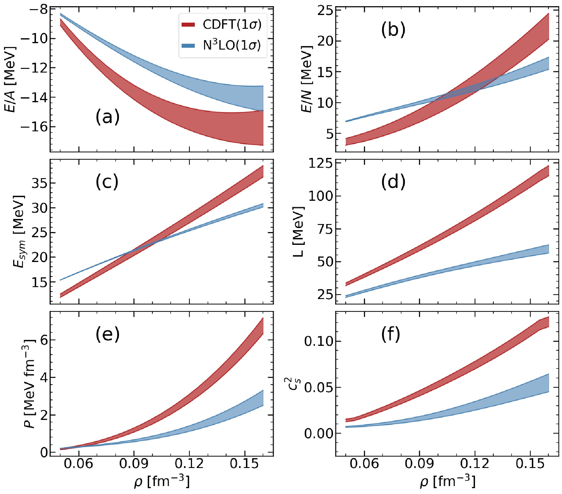
Figure 4. (color online) (a) The energy per particle
$ E/A $ for symmetric nuclear matter, (b) the energy per neutron$ E/N $ for pure neutron matter, (c) the symmetry energy$ E_{\rm sym} $ , (d) the symmetry energy slope L, (e) the pressure P, and (f) the square of the speed of sound$ c_s^2 $ are calculated using approximately one million samples from the covariant EDF. The results are compared with those, labeled as N3LO, from ab initio many-body perturbation theory calculations based on a chiral Hamiltonian by Drischler et al. [90].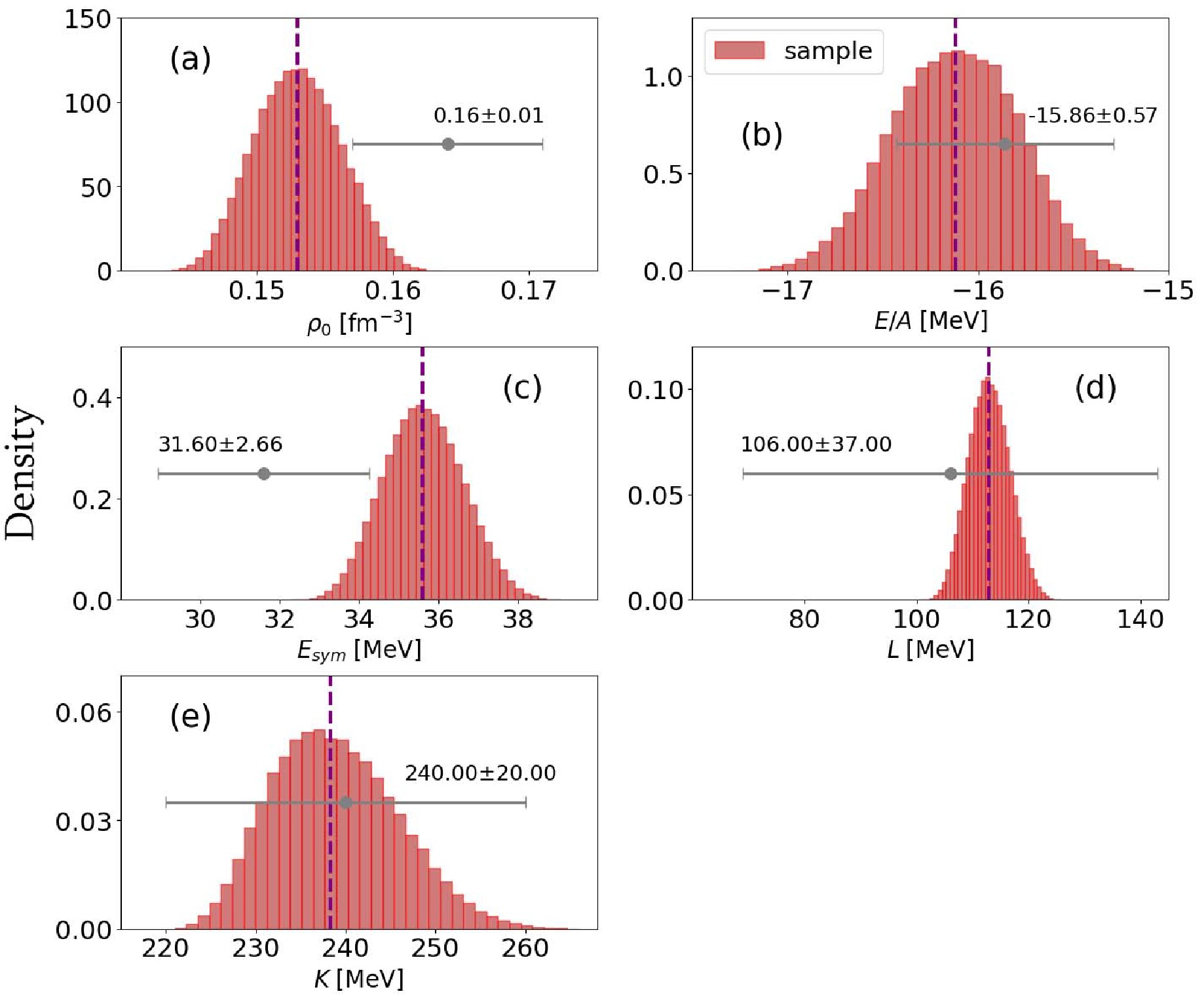
Figure 5. (color online) Histograms of nuclear-matter properties around saturation density calculated using
$ (9+1)\times 2^{17}= $ $ 1310720 $ quasi-MC samples of the nine coupling constants in the relativistic EDFs around the PC-PK1 parametrization [79]. The empirical values (gray error bars) are shown for comparison.$ I_{(i)}({\boldsymbol{C}}) =\sqrt{\dfrac{\left[O^{\rm calc.}_{(i)}({\boldsymbol{C}})-O^{\rm empi.}_{(i)}\right]^{2}}{ \sigma^2\left(O^{\rm empi.}_{(i)}\right)}}. $
(37) Here,
$ \sigma\left(O^{\rm empi.}{(i)}\right) $ denotes the standard deviation of the empirical value for the i-th physical quantity of infinite nuclear matter. The implausibility function$ I{(i)}(x) $ quantifies the probability that the theoretically calculated value$ O^{\rm calc.}{(i)}(x) $ matches the empirical value$ O^{\rm empi.}{(i)} $ . We screen the parameter sets C using the criterion$ \max[I_{(i)}(x)] \lt \sqrt{3} $ , which corresponds to a probability of approximately 92%. Here,$ \max[I_{(i)}(x)] $ represents the largest value of the implausibility functions across the physical quantities$ \Theta_{\rm sat} $ of infinite nuclear matter. After applying the$ \sqrt{3}\sigma $ screening rule based on the properties of nuclear matter, we obtain a final set of 457,380 non-implausible samples. -
The single-particle state in infinite nuclear matter is labeled by the momentum
$ {\boldsymbol{p}}=\hbar{\boldsymbol{k}} $ and the spin direction λ. The corresponding single-particle wave function reduces to$ u_\tau({\boldsymbol{k}},\lambda) $ , which satisfies the following Dirac equation:$ \left({\boldsymbol{\alpha}}\cdot{\boldsymbol{k}} + \beta M^*_\tau +\Sigma_{\tau}^{0}\right)u_\tau({\boldsymbol{k}},\lambda) = E_\tau({\boldsymbol{k}}) u_\tau({\boldsymbol{k}},\lambda), $
(31) where
$ \tau(n,\; p) $ distinguishes neutrons and protons,$ M^*_\tau = M_\tau + \Sigma_{\tau S} $ is the Dirac mass. The nucleon self-energies are determined by the scalar and vector densities$ \Sigma_{\tau S} = \alpha_S\rho_S+\beta_S\rho_S^2 +\gamma_S \rho_S^3, $
(32a) $ \Sigma_{\tau}^{0}=\alpha_V\rho_V +\gamma_V\rho^3_V + \alpha_{TV}\tau_3\rho_{TV}, $
(32b) where
$ \rho_i = \rho^{(n)}_i + \rho^{(p)}_i $ with$ i = S, V $ labeling the scalar and vector densities, respectively. The isovector density is defined as the difference between the neutron and proton number densities,$ \rho_{TV} = \rho^{(n)}_V - \rho^{(p)}_V $ . All densities are constant for uniformly distributed nuclear matter, for which all derivative terms depending on the parameters$ \delta_{S, V, TV} $ vanish. For neutrons ($ \tau = n $ ) and protons ($ \tau = p $ ), the scalar density ($ \rho_S $ ) and time-like component ($ \rho_V $ ) of the vector densities$ j^\mu_V $ are calculated$ \rho^{(\tau)}_{S} =\sum\limits_\lambda\int^{k_{\tau F}} \dfrac{{\mathrm{d}}^3k}{(2\pi)^3} \dfrac{M^*_\tau} {E_\tau^*({\boldsymbol{k}})} , $
(33a) $ \rho^{(\tau)}_{V} =\sum\limits_\lambda\int^{k_{\tau F}} \dfrac{{\mathrm{d}}^3k}{(2\pi)^3}=\dfrac{k_{\tau F}^3} {3\pi^2}, $
(33b) where
$ E_{\tau F}^* = \sqrt{M^{*2}_\tau + k_{\tau F}^2} $ , and λ runs over spin up and down, yielding a factor of two. At zero temperature, the energy density and pressure of nuclear matter are given by [89]$\begin{aligned}[b] \varepsilon= \sum_\tau\left[\frac{3}{4}\left(\rho_V^{(\tau)} E_{\tau F}^*-\rho_S^{(\tau)} M_\tau^*\right)+\rho_V^{(\tau)} M_\tau\right] \end{aligned} $
$\begin{aligned}[b] & +\frac{\alpha_S}{2} \rho_S^2+\frac{\beta_S}{3} \rho_S^3+\frac{\gamma_S}{4} \rho_S^4+\frac{\alpha_V}{2} \rho_V^2\\& +\frac{\gamma_V}{4} \rho_V^4+\frac{\alpha_{T V}}{2} \rho_{T V}^2,\end{aligned} $
(34a) $\begin{aligned}[b] p =& \sum\limits_\tau\left[\dfrac{1}{4}\left(\rho^{(\tau)}_{V}E_{\tau F}^* -\rho^{(\tau)}_{ S}M_\tau^*\right)+\Sigma_{\tau 0}\rho^{(\tau)}_{V} +\Sigma_{\tau S} \rho^{(\tau)}_{S}\right] \\&-\dfrac{\alpha_S}{2}\rho_S^2-\dfrac{\beta_S}{3}\rho_S^3- \dfrac{\gamma_S}{4}\rho_S^4- \dfrac{\alpha_V}{2}\rho^2_V\\& - \dfrac{\gamma_V}{4}\rho^4_V - \dfrac{\alpha_{TV}}{2}\rho_{TV}^2.\end{aligned} $
(34b) The average nucleon binding energy
$ E/A $ and incompressibility K are defined as$ E/A \equiv \varepsilon/\rho_V -M,\quad K \equiv 9\dfrac{\partial p}{\partial \rho_V}. $
(35) In addition, the symmetry energy
$ E_\mathrm{sym} $ and its slope parameter L are calculated by$ E_\mathrm{sym} \equiv \dfrac{1}{2}\left.\dfrac{\partial^2 (E/A)} {\partial \eta^2}\right|_{\eta=0},\qquad L \equiv 3\rho \dfrac{\partial E_\mathrm{sym}}{\partial \rho_V}, $
(36) with the isospin asymmetry
$ \eta = \rho_{TV}/\rho_V $ . The speed of sound is defined as$ c_s=\sqrt{\partial p/\partial \epsilon} $ [90], in units of the speed of light c.We sampled a total of
$ (9+1) \times 2^{17} \approx 1.3 \times 10^6 $ EDF parameter sets by varying all nine parameters around the PC-PK1 values [79] using quasi Monte Carlo (MC) sampling with a uniform distribution within the ranges shown in Table 2. This quasi-MC sampling method has been widely employed in statistical analyses of large-scale datasets, including global sensitivity analysis [67] and uncertainty quantification. Using these parameter sets, we calculated the properties of infinite nuclear matter as a function of nucleon number density$ \rho_V $ , as illustrated in Fig. 4. For comparison, results from many-body perturbation theory based on a chiral Hamiltonian [90] are also presented, revealing significant discrepancies between the two approaches. The physical quantities at saturation density,$ \Theta_{\rm sat} = \{\rho_0, E/A, E_{\rm sym}, L, K\} $ , calculated from the sampled EDF parameter sets are displayed in Fig. 5. We observe some mismatches between the mean values of$ \rho_0 $ and$ E_{\rm sym} $ and their empirical values. To incorporate refinements from nuclear matter into the EDFs, we introduce the implausibility function [91]$ c_\ell $ PC-PK1 [79] Dimension Training sets[%] Target sets[%] $ \alpha_S $ −3.96291 $ \times 10^{-4} $ ${\rm{MeV}} ^{-2} $ 0.5 0.1 $ \beta_S $ +8.6653 $ \times 10^{-11} $ ${\rm{MeV}} ^{-5} $ 2 1 $ \gamma_S $ −3.80724 $ \times 10^{-17} $ ${\rm{MeV}} ^{-8} $ 4 2 $ \delta_S $ −1.09108 $ \times 10^{-10} $ ${\rm{MeV}} ^{-4} $ 20 4 $ \alpha_V $ +2.69040 $ \times 10^{-4} $ ${\rm{MeV}} ^{-2} $ 0.8 0.2 $ \gamma_V $ −3.64219 $ \times 10^{-18} $ ${\rm{MeV}} ^{-8} $ 30 5 $ \delta_V $ −4.32619 $ \times 10^{-10} $ ${\rm{MeV}} ^{-4} $ 20 5 $ \alpha_{TV} $ +2.95018 $ \times 10^{-5} $ ${\rm{MeV}} ^{-2} $ 10 6 $ \delta_{TV} $ −4.11112 $ \times 10^{-10} $ ${\rm{MeV}} ^{-4} $ 150 40 Table 2. The values of the PC-PK1 parameter set of the relativistic EDF and the parameter ranges in the training and target sets.
Figure 4. (color online) (a) The energy per particle
$ E/A $ for symmetric nuclear matter, (b) the energy per neutron$ E/N $ for pure neutron matter, (c) the symmetry energy$ E_{\rm sym} $ , (d) the symmetry energy slope L, (e) the pressure P, and (f) the square of the speed of sound$ c_s^2 $ are calculated using approximately one million samples from the covariant EDF. The results are compared with those, labeled as N3LO, from ab initio many-body perturbation theory calculations based on a chiral Hamiltonian by Drischler et al. [90].
Figure 5. (color online) Histograms of nuclear-matter properties around saturation density calculated using
$ (9+1)\times 2^{17}= $ $ 1310720 $ quasi-MC samples of the nine coupling constants in the relativistic EDFs around the PC-PK1 parametrization [79]. The empirical values (gray error bars) are shown for comparison.$ I_{(i)}({\boldsymbol{C}}) =\sqrt{\dfrac{\left[O^{\rm calc.}_{(i)}({\boldsymbol{C}})-O^{\rm empi.}_{(i)}\right]^{2}}{ \sigma^2\left(O^{\rm empi.}_{(i)}\right)}}. $
(37) Here,
$ \sigma\left(O^{\rm empi.}{(i)}\right) $ denotes the standard deviation of the empirical value for the i-th physical quantity of infinite nuclear matter. The implausibility function$ I{(i)}(x) $ quantifies the probability that the theoretically calculated value$ O^{\rm calc.}{(i)}(x) $ matches the empirical value$ O^{\rm empi.}{(i)} $ . We screen the parameter sets C using the criterion$ \max[I_{(i)}(x)] \lt \sqrt{3} $ , which corresponds to a probability of approximately 92%. Here,$ \max[I_{(i)}(x)] $ represents the largest value of the implausibility functions across the physical quantities$ \Theta_{\rm sat} $ of infinite nuclear matter. After applying the$ \sqrt{3}\sigma $ screening rule based on the properties of nuclear matter, we obtain a final set of 457,380 non-implausible samples. -
The single-particle state in infinite nuclear matter is labeled by the momentum
$ {\boldsymbol{p}}=\hbar{\boldsymbol{k}} $ and the spin direction λ. The corresponding single-particle wave function reduces to$ u_\tau({\boldsymbol{k}},\lambda) $ , which satisfies the following Dirac equation:$ \left({\boldsymbol{\alpha}}\cdot{\boldsymbol{k}} + \beta M^*_\tau +\Sigma_{\tau}^{0}\right)u_\tau({\boldsymbol{k}},\lambda) = E_\tau({\boldsymbol{k}}) u_\tau({\boldsymbol{k}},\lambda), $
(31) where
$ \tau(n,\; p) $ distinguishes neutrons and protons,$ M^*_\tau = M_\tau + \Sigma_{\tau S} $ is the Dirac mass. The nucleon self-energies are determined by the scalar and vector densities$ \Sigma_{\tau S} = \alpha_S\rho_S+\beta_S\rho_S^2 +\gamma_S \rho_S^3, $
(32a) $ \Sigma_{\tau}^{0}=\alpha_V\rho_V +\gamma_V\rho^3_V + \alpha_{TV}\tau_3\rho_{TV}, $
(32b) where
$ \rho_i = \rho^{(n)}_i + \rho^{(p)}_i $ with$ i = S, V $ labeling the scalar and vector densities, respectively. The isovector density is defined as the difference between the neutron and proton number densities,$ \rho_{TV} = \rho^{(n)}_V - \rho^{(p)}_V $ . All densities are constant for uniformly distributed nuclear matter, for which all derivative terms depending on the parameters$ \delta_{S, V, TV} $ vanish. For neutrons ($ \tau = n $ ) and protons ($ \tau = p $ ), the scalar density ($ \rho_S $ ) and time-like component ($ \rho_V $ ) of the vector densities$ j^\mu_V $ are calculated$ \rho^{(\tau)}_{S} =\sum\limits_\lambda\int^{k_{\tau F}} \dfrac{{\mathrm{d}}^3k}{(2\pi)^3} \dfrac{M^*_\tau} {E_\tau^*({\boldsymbol{k}})} , $
(33a) $ \rho^{(\tau)}_{V} =\sum\limits_\lambda\int^{k_{\tau F}} \dfrac{{\mathrm{d}}^3k}{(2\pi)^3}=\dfrac{k_{\tau F}^3} {3\pi^2}, $
(33b) where
$ E_{\tau F}^* = \sqrt{M^{*2}_\tau + k_{\tau F}^2} $ , and λ runs over spin up and down, yielding a factor of two. At zero temperature, the energy density and pressure of nuclear matter are given by [89]$\begin{aligned}[b] \varepsilon= \sum_\tau\left[\frac{3}{4}\left(\rho_V^{(\tau)} E_{\tau F}^*-\rho_S^{(\tau)} M_\tau^*\right)+\rho_V^{(\tau)} M_\tau\right] \end{aligned} $
$\begin{aligned}[b] & +\frac{\alpha_S}{2} \rho_S^2+\frac{\beta_S}{3} \rho_S^3+\frac{\gamma_S}{4} \rho_S^4+\frac{\alpha_V}{2} \rho_V^2\\& +\frac{\gamma_V}{4} \rho_V^4+\frac{\alpha_{T V}}{2} \rho_{T V}^2,\end{aligned} $
(34a) $\begin{aligned}[b] p =& \sum\limits_\tau\left[\dfrac{1}{4}\left(\rho^{(\tau)}_{V}E_{\tau F}^* -\rho^{(\tau)}_{ S}M_\tau^*\right)+\Sigma_{\tau 0}\rho^{(\tau)}_{V} +\Sigma_{\tau S} \rho^{(\tau)}_{S}\right] \\&-\dfrac{\alpha_S}{2}\rho_S^2-\dfrac{\beta_S}{3}\rho_S^3- \dfrac{\gamma_S}{4}\rho_S^4- \dfrac{\alpha_V}{2}\rho^2_V\\& - \dfrac{\gamma_V}{4}\rho^4_V - \dfrac{\alpha_{TV}}{2}\rho_{TV}^2.\end{aligned} $
(34b) The average nucleon binding energy
$ E/A $ and incompressibility K are defined as$ E/A \equiv \varepsilon/\rho_V -M,\quad K \equiv 9\dfrac{\partial p}{\partial \rho_V}. $
(35) In addition, the symmetry energy
$ E_\mathrm{sym} $ and its slope parameter L are calculated by$ E_\mathrm{sym} \equiv \dfrac{1}{2}\left.\dfrac{\partial^2 (E/A)} {\partial \eta^2}\right|_{\eta=0},\qquad L \equiv 3\rho \dfrac{\partial E_\mathrm{sym}}{\partial \rho_V}, $
(36) with the isospin asymmetry
$ \eta = \rho_{TV}/\rho_V $ . The speed of sound is defined as$ c_s=\sqrt{\partial p/\partial \epsilon} $ [90], in units of the speed of light c.We sampled a total of
$ (9+1) \times 2^{17} \approx 1.3 \times 10^6 $ EDF parameter sets by varying all nine parameters around the PC-PK1 values [79] using quasi Monte Carlo (MC) sampling with a uniform distribution within the ranges shown in Table 2. This quasi-MC sampling method has been widely employed in statistical analyses of large-scale datasets, including global sensitivity analysis [67] and uncertainty quantification. Using these parameter sets, we calculated the properties of infinite nuclear matter as a function of nucleon number density$ \rho_V $ , as illustrated in Fig. 4. For comparison, results from many-body perturbation theory based on a chiral Hamiltonian [90] are also presented, revealing significant discrepancies between the two approaches. The physical quantities at saturation density,$ \Theta_{\rm sat} = \{\rho_0, E/A, E_{\rm sym}, L, K\} $ , calculated from the sampled EDF parameter sets are displayed in Fig. 5. We observe some mismatches between the mean values of$ \rho_0 $ and$ E_{\rm sym} $ and their empirical values. To incorporate refinements from nuclear matter into the EDFs, we introduce the implausibility function [91]$ c_\ell $ PC-PK1 [79] Dimension Training sets[%] Target sets[%] $ \alpha_S $ −3.96291 $ \times 10^{-4} $ ${\rm{MeV}} ^{-2} $ 0.5 0.1 $ \beta_S $ +8.6653 $ \times 10^{-11} $ ${\rm{MeV}} ^{-5} $ 2 1 $ \gamma_S $ −3.80724 $ \times 10^{-17} $ ${\rm{MeV}} ^{-8} $ 4 2 $ \delta_S $ −1.09108 $ \times 10^{-10} $ ${\rm{MeV}} ^{-4} $ 20 4 $ \alpha_V $ +2.69040 $ \times 10^{-4} $ ${\rm{MeV}} ^{-2} $ 0.8 0.2 $ \gamma_V $ −3.64219 $ \times 10^{-18} $ ${\rm{MeV}} ^{-8} $ 30 5 $ \delta_V $ −4.32619 $ \times 10^{-10} $ ${\rm{MeV}} ^{-4} $ 20 5 $ \alpha_{TV} $ +2.95018 $ \times 10^{-5} $ ${\rm{MeV}} ^{-2} $ 10 6 $ \delta_{TV} $ −4.11112 $ \times 10^{-10} $ ${\rm{MeV}} ^{-4} $ 150 40 Table 2. The values of the PC-PK1 parameter set of the relativistic EDF and the parameter ranges in the training and target sets.
Figure 4. (color online) (a) The energy per particle
$ E/A $ for symmetric nuclear matter, (b) the energy per neutron$ E/N $ for pure neutron matter, (c) the symmetry energy$ E_{\rm sym} $ , (d) the symmetry energy slope L, (e) the pressure P, and (f) the square of the speed of sound$ c_s^2 $ are calculated using approximately one million samples from the covariant EDF. The results are compared with those, labeled as N3LO, from ab initio many-body perturbation theory calculations based on a chiral Hamiltonian by Drischler et al. [90].
Figure 5. (color online) Histograms of nuclear-matter properties around saturation density calculated using
$ (9+1)\times 2^{17}= $ $ 1310720 $ quasi-MC samples of the nine coupling constants in the relativistic EDFs around the PC-PK1 parametrization [79]. The empirical values (gray error bars) are shown for comparison.$ I_{(i)}({\boldsymbol{C}}) =\sqrt{\dfrac{\left[O^{\rm calc.}_{(i)}({\boldsymbol{C}})-O^{\rm empi.}_{(i)}\right]^{2}}{ \sigma^2\left(O^{\rm empi.}_{(i)}\right)}}. $
(37) Here,
$ \sigma\left(O^{\rm empi.}{(i)}\right) $ denotes the standard deviation of the empirical value for the i-th physical quantity of infinite nuclear matter. The implausibility function$ I{(i)}(x) $ quantifies the probability that the theoretically calculated value$ O^{\rm calc.}{(i)}(x) $ matches the empirical value$ O^{\rm empi.}{(i)} $ . We screen the parameter sets C using the criterion$ \max[I_{(i)}(x)] \lt \sqrt{3} $ , which corresponds to a probability of approximately 92%. Here,$ \max[I_{(i)}(x)] $ represents the largest value of the implausibility functions across the physical quantities$ \Theta_{\rm sat} $ of infinite nuclear matter. After applying the$ \sqrt{3}\sigma $ screening rule based on the properties of nuclear matter, we obtain a final set of 457,380 non-implausible samples. -
The single-particle state in infinite nuclear matter is labeled by the momentum
$ {\boldsymbol{p}}=\hbar{\boldsymbol{k}} $ and the spin direction λ. The corresponding single-particle wave function reduces to$ u_\tau({\boldsymbol{k}},\lambda) $ , which satisfies the following Dirac equation:$ \left({\boldsymbol{\alpha}}\cdot{\boldsymbol{k}} + \beta M^*_\tau +\Sigma_{\tau}^{0}\right)u_\tau({\boldsymbol{k}},\lambda) = E_\tau({\boldsymbol{k}}) u_\tau({\boldsymbol{k}},\lambda), $
(31) where
$ \tau(n,\; p) $ distinguishes neutrons and protons,$ M^*_\tau = M_\tau + \Sigma_{\tau S} $ is the Dirac mass. The nucleon self-energies are determined by the scalar and vector densities$ \Sigma_{\tau S} = \alpha_S\rho_S+\beta_S\rho_S^2 +\gamma_S \rho_S^3, $
(32a) $ \Sigma_{\tau}^{0}=\alpha_V\rho_V +\gamma_V\rho^3_V + \alpha_{TV}\tau_3\rho_{TV}, $
(32b) where
$ \rho_i = \rho^{(n)}_i + \rho^{(p)}_i $ with$ i = S, V $ labeling the scalar and vector densities, respectively. The isovector density is defined as the difference between the neutron and proton number densities,$ \rho_{TV} = \rho^{(n)}_V - \rho^{(p)}_V $ . All densities are constant for uniformly distributed nuclear matter, for which all derivative terms depending on the parameters$ \delta_{S, V, TV} $ vanish. For neutrons ($ \tau = n $ ) and protons ($ \tau = p $ ), the scalar density ($ \rho_S $ ) and time-like component ($ \rho_V $ ) of the vector densities$ j^\mu_V $ are calculated$ \rho^{(\tau)}_{S} =\sum\limits_\lambda\int^{k_{\tau F}} \dfrac{{\mathrm{d}}^3k}{(2\pi)^3} \dfrac{M^*_\tau} {E_\tau^*({\boldsymbol{k}})} , $
(33a) $ \rho^{(\tau)}_{V} =\sum\limits_\lambda\int^{k_{\tau F}} \dfrac{{\mathrm{d}}^3k}{(2\pi)^3}=\dfrac{k_{\tau F}^3} {3\pi^2}, $
(33b) where
$ E_{\tau F}^* = \sqrt{M^{*2}_\tau + k_{\tau F}^2} $ , and λ runs over spin up and down, yielding a factor of two. At zero temperature, the energy density and pressure of nuclear matter are given by [89]$\begin{aligned}[b] \varepsilon= \sum_\tau\left[\frac{3}{4}\left(\rho_V^{(\tau)} E_{\tau F}^*-\rho_S^{(\tau)} M_\tau^*\right)+\rho_V^{(\tau)} M_\tau\right] \end{aligned} $
$\begin{aligned}[b] & +\frac{\alpha_S}{2} \rho_S^2+\frac{\beta_S}{3} \rho_S^3+\frac{\gamma_S}{4} \rho_S^4+\frac{\alpha_V}{2} \rho_V^2\\& +\frac{\gamma_V}{4} \rho_V^4+\frac{\alpha_{T V}}{2} \rho_{T V}^2,\end{aligned} $
(34a) $\begin{aligned}[b] p =& \sum\limits_\tau\left[\dfrac{1}{4}\left(\rho^{(\tau)}_{V}E_{\tau F}^* -\rho^{(\tau)}_{ S}M_\tau^*\right)+\Sigma_{\tau 0}\rho^{(\tau)}_{V} +\Sigma_{\tau S} \rho^{(\tau)}_{S}\right] \\&-\dfrac{\alpha_S}{2}\rho_S^2-\dfrac{\beta_S}{3}\rho_S^3- \dfrac{\gamma_S}{4}\rho_S^4- \dfrac{\alpha_V}{2}\rho^2_V\\& - \dfrac{\gamma_V}{4}\rho^4_V - \dfrac{\alpha_{TV}}{2}\rho_{TV}^2.\end{aligned} $
(34b) The average nucleon binding energy
$ E/A $ and incompressibility K are defined as$ E/A \equiv \varepsilon/\rho_V -M,\quad K \equiv 9\dfrac{\partial p}{\partial \rho_V}. $
(35) In addition, the symmetry energy
$ E_\mathrm{sym} $ and its slope parameter L are calculated by$ E_\mathrm{sym} \equiv \dfrac{1}{2}\left.\dfrac{\partial^2 (E/A)} {\partial \eta^2}\right|_{\eta=0},\qquad L \equiv 3\rho \dfrac{\partial E_\mathrm{sym}}{\partial \rho_V}, $
(36) with the isospin asymmetry
$ \eta = \rho_{TV}/\rho_V $ . The speed of sound is defined as$ c_s=\sqrt{\partial p/\partial \epsilon} $ [90], in units of the speed of light c.We sampled a total of
$ (9+1) \times 2^{17} \approx 1.3 \times 10^6 $ EDF parameter sets by varying all nine parameters around the PC-PK1 values [79] using quasi Monte Carlo (MC) sampling with a uniform distribution within the ranges shown in Table 2. This quasi-MC sampling method has been widely employed in statistical analyses of large-scale datasets, including global sensitivity analysis [67] and uncertainty quantification. Using these parameter sets, we calculated the properties of infinite nuclear matter as a function of nucleon number density$ \rho_V $ , as illustrated in Fig. 4. For comparison, results from many-body perturbation theory based on a chiral Hamiltonian [90] are also presented, revealing significant discrepancies between the two approaches. The physical quantities at saturation density,$ \Theta_{\rm sat} = \{\rho_0, E/A, E_{\rm sym}, L, K\} $ , calculated from the sampled EDF parameter sets are displayed in Fig. 5. We observe some mismatches between the mean values of$ \rho_0 $ and$ E_{\rm sym} $ and their empirical values. To incorporate refinements from nuclear matter into the EDFs, we introduce the implausibility function [91]$ c_\ell $ PC-PK1 [79] Dimension Training sets[%] Target sets[%] $ \alpha_S $ −3.96291 $ \times 10^{-4} $ ${\rm{MeV}} ^{-2} $ 0.5 0.1 $ \beta_S $ +8.6653 $ \times 10^{-11} $ ${\rm{MeV}} ^{-5} $ 2 1 $ \gamma_S $ −3.80724 $ \times 10^{-17} $ ${\rm{MeV}} ^{-8} $ 4 2 $ \delta_S $ −1.09108 $ \times 10^{-10} $ ${\rm{MeV}} ^{-4} $ 20 4 $ \alpha_V $ +2.69040 $ \times 10^{-4} $ ${\rm{MeV}} ^{-2} $ 0.8 0.2 $ \gamma_V $ −3.64219 $ \times 10^{-18} $ ${\rm{MeV}} ^{-8} $ 30 5 $ \delta_V $ −4.32619 $ \times 10^{-10} $ ${\rm{MeV}} ^{-4} $ 20 5 $ \alpha_{TV} $ +2.95018 $ \times 10^{-5} $ ${\rm{MeV}} ^{-2} $ 10 6 $ \delta_{TV} $ −4.11112 $ \times 10^{-10} $ ${\rm{MeV}} ^{-4} $ 150 40 Table 2. The values of the PC-PK1 parameter set of the relativistic EDF and the parameter ranges in the training and target sets.
Figure 4. (color online) (a) The energy per particle
$ E/A $ for symmetric nuclear matter, (b) the energy per neutron$ E/N $ for pure neutron matter, (c) the symmetry energy$ E_{\rm sym} $ , (d) the symmetry energy slope L, (e) the pressure P, and (f) the square of the speed of sound$ c_s^2 $ are calculated using approximately one million samples from the covariant EDF. The results are compared with those, labeled as N3LO, from ab initio many-body perturbation theory calculations based on a chiral Hamiltonian by Drischler et al. [90].
Figure 5. (color online) Histograms of nuclear-matter properties around saturation density calculated using
$ (9+1)\times 2^{17}= $ $ 1310720 $ quasi-MC samples of the nine coupling constants in the relativistic EDFs around the PC-PK1 parametrization [79]. The empirical values (gray error bars) are shown for comparison.$ I_{(i)}({\boldsymbol{C}}) =\sqrt{\dfrac{\left[O^{\rm calc.}_{(i)}({\boldsymbol{C}})-O^{\rm empi.}_{(i)}\right]^{2}}{ \sigma^2\left(O^{\rm empi.}_{(i)}\right)}}. $
(37) Here,
$ \sigma\left(O^{\rm empi.}{(i)}\right) $ denotes the standard deviation of the empirical value for the i-th physical quantity of infinite nuclear matter. The implausibility function$ I{(i)}(x) $ quantifies the probability that the theoretically calculated value$ O^{\rm calc.}{(i)}(x) $ matches the empirical value$ O^{\rm empi.}{(i)} $ . We screen the parameter sets C using the criterion$ \max[I_{(i)}(x)] \lt \sqrt{3} $ , which corresponds to a probability of approximately 92%. Here,$ \max[I_{(i)}(x)] $ represents the largest value of the implausibility functions across the physical quantities$ \Theta_{\rm sat} $ of infinite nuclear matter. After applying the$ \sqrt{3}\sigma $ screening rule based on the properties of nuclear matter, we obtain a final set of 457,380 non-implausible samples. -
Using the above non-implausible samples, we calculated the physical quantities of low-lying nuclear states with SP-CDFT(14,
$ k_{\rm max} $ ) for 150Nd, 150Sm, 136Xe, and 136Ba. The results for 136Xe and 150Nd, with and without refinement from nuclear matter properties, are shown in red and blue in Fig. 6. Because the results for 150Sm closely resemble those for 150Nd, and those for 136Ba are similar to 136Xe, we do not display them here. As shown in the figure, the ground-state energy is only weakly correlated with the excitation energies of the$ 2^+_1 $ and$ 4^+_1 $ states, as well as with the corresponding$ E2 $ transition strengths, and this weak correlation appears to be nucleus-dependent. In contrast, the ground-state energy (or equivalently, the binding energy with the opposite sign) is strongly positively (or negatively) correlated with the proton rms radius in both spherical and deformed nuclei. This suggests that the correlation is not primarily driven by deformation, but rather by changes in the nuclear-matter equation of state (EOS): parameter sets that yield larger ground-state binding energies tend to correspond to larger saturation densities$ \rho_0 $ and smaller proton rms radii$ R_p $ , as shown in Ref. [60].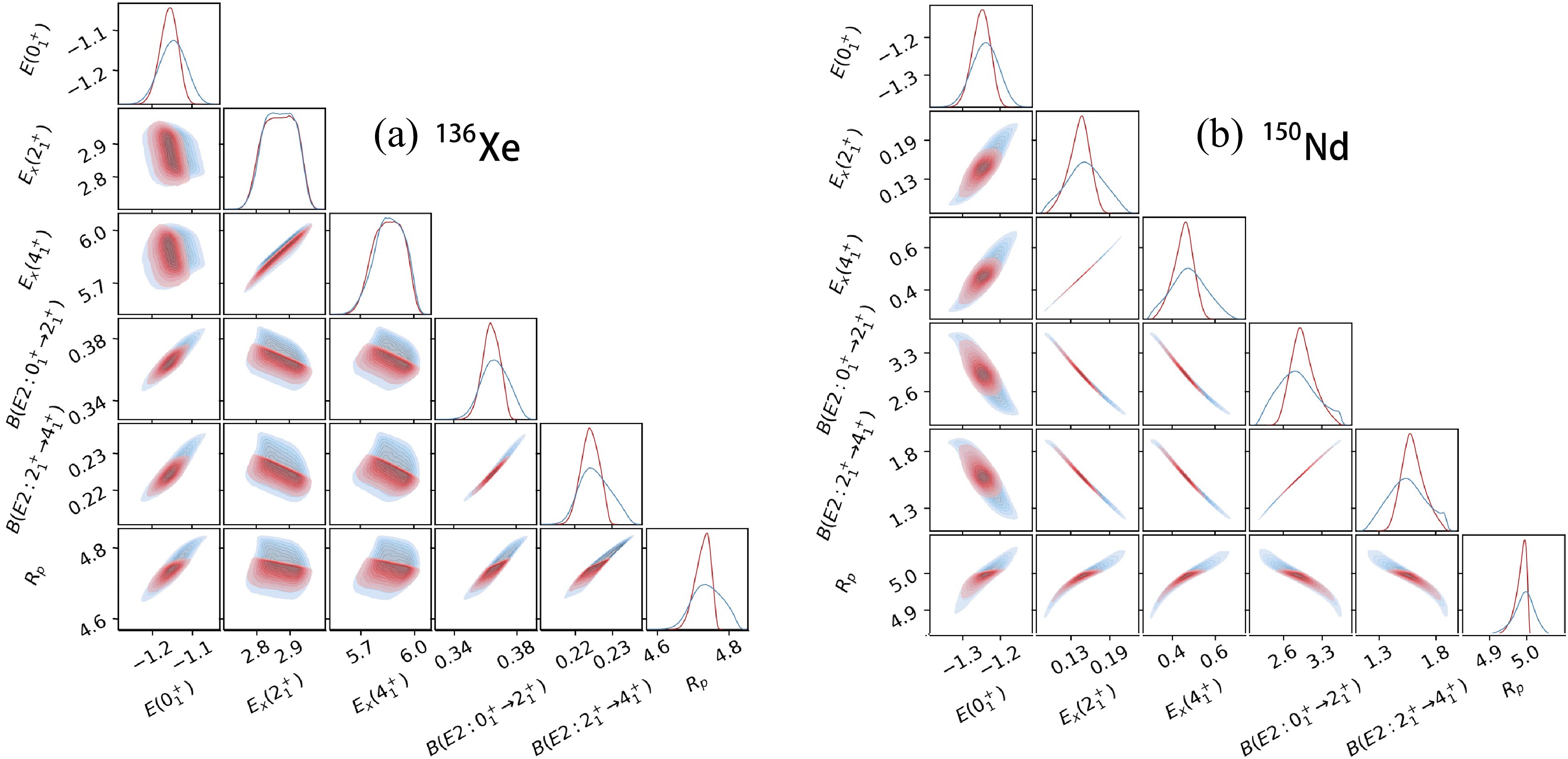
Figure 6. (color online) Correlations between different quantities of low-lying states. The diagonal panels show histograms of the probability distributions of these quantities for (a) 136Xe and (b) 150Nd. The red distributions are refined by the empirical values of the physical quantities
$ \Theta_{\rm sat}=\{\rho_0, E/A, E_{\rm sym}, L, K\} $ for infinite nuclear matter at saturation density using the$ \sqrt{3}\sigma $ rule. The black circles denote experimental values taken from [92]. See the main text for details.Moreover, the excitation energies of the
$ 2^+_1 $ and$ 4^+_1 $ states and the corresponding$ E2 $ transition strengths among them are governed by quadrupole deformation. Figure 6 clearly shows that the excitation energies and$ B(E2) $ values are strongly anticorrelated with each other in both nuclei, confirming that these correlations are dominated by the deformation effect. This correlation is stronger in the deformed nucleus 150Nd than in 136Xe. In particular, the proton radius$ R_p $ of the ground state is positively correlated with$ B(E2: 0^+_1 \to 2^+_1) $ in 136Xe, whereas it is anticorrelated in 150Nd. This further confirms that the variation of$ R_p $ is not dominated by quadrupole deformation, but by changes in the EOS.To understand the anticorrelation in 150Nd, we plot the unnormalized mean-squared radii
$ \bar{R}_p^2 $ against the unnormalized reduced$ E2 $ transition matrix element$ |\bar{Q}_p| $ from single-configuration calculations using different EDF parameter sets in Fig. 7. These quantities are strongly positively correlated, as expected. Because the normalization factor$ \sqrt{N_0} $ of the$ J=0 $ state is linearly correlated with the normalization factor$ \sqrt{N_2} $ of the$ J=2 $ state with a nonzero intercept, an anticorrelation arises between the normalized mean-squared radii$ R_p^2 $ and the normalized reduced$ E2 $ transition matrix element$ |Q_p| $ , as illustrated in Fig. 7(c). This anticorrelation persists in the configuration-mixing GCM calculation, as shown in Fig. 7(d). In short,$ B(E2: 0^+_1 \to 2^+_1) $ can be either positively or negatively correlated with the proton radius$ R_p $ of the ground state.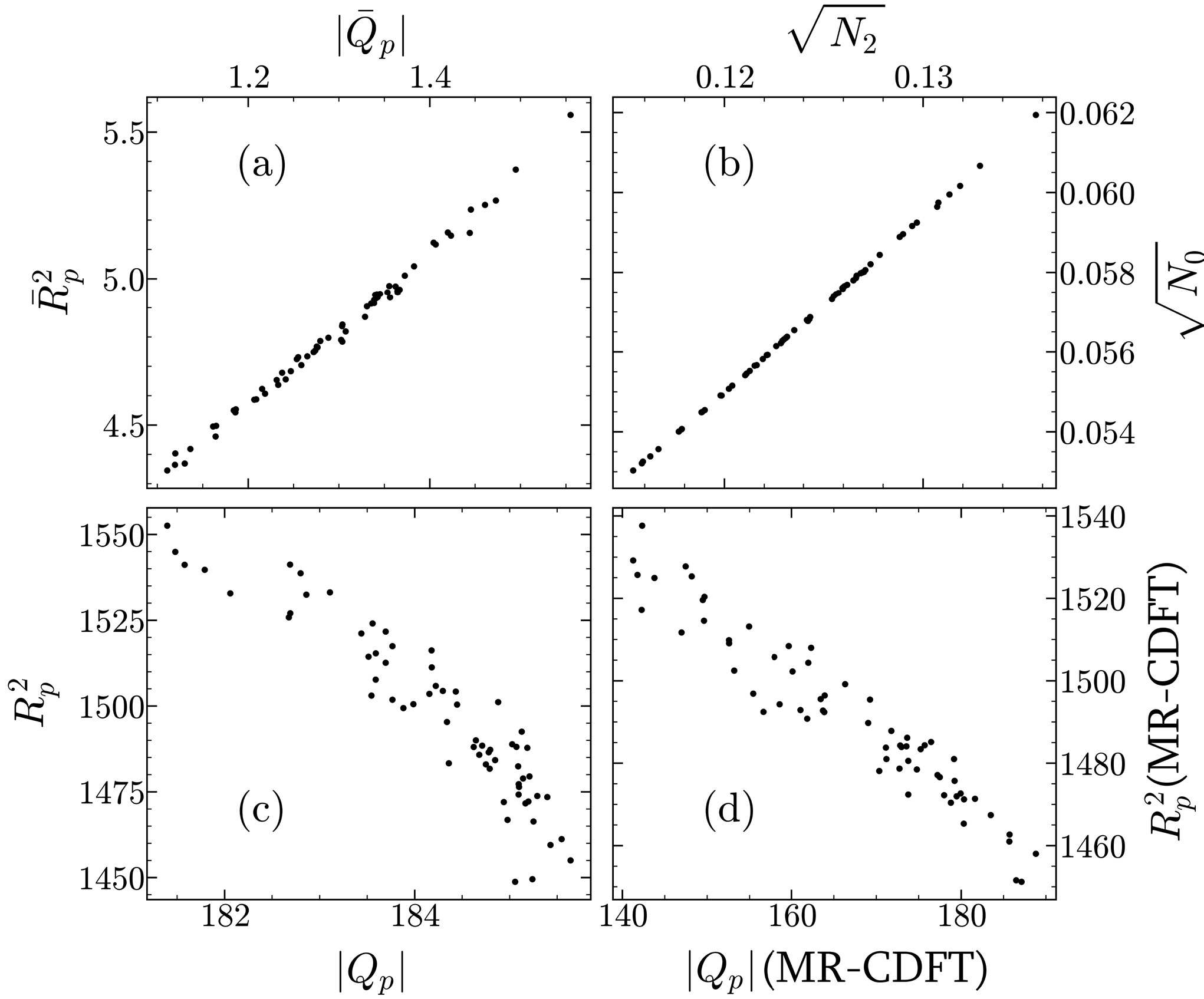
Figure 7. (a), (b), (c) Correlations among the mean-squared radius
$ R_p^2=N^{-1}_0\left\langle {J=0NZ;\beta_2,{\bf{C}}}\right|\hat R^2_p\left| {J=0NZ;\beta_2,{\bf{C}}}\right\rangle $ , the reduced$ E2 $ transition matrix element$ Q_p=(N_0N_2)^{-1/2}\left\langle J=2NZ;\beta_2, \right. $ $ \left. {\bf{C}}\right||\hat Q_2|\left| {J=0NZ;\beta_2,{\bf{C}}}\right\rangle $ , and the normalization factors$ \sqrt{N_{J}} $ from calculations for 150Nd based on a single configuration with$ \beta_2=0.3 $ , where$ N_J=\left\langle {JNZ;\beta_2,{\bf{C}}}\right|JNZ;\beta_2,{\bf{C}}\rangle $ . (d) Results from configuration-mixing MR-CDFT calculations. The quantities denoted with bars are unnormalized.Subsequently, we use the Bayesian method to derive the posterior distribution
$ p({\cal{O}}|{\cal{D}}) $ for the quantity$ {\cal{O}} $ given the data$ {\cal{D}} $ . The true value$ {\cal{O}}^{(\rm{true})} $ of$ {\cal{O}} $ can be decomposed as follows [93],$ {\cal{O}}^{(\rm{true})} ={\cal{O}}^{(\rm{MR-CDFT})}({\boldsymbol{C}}) +\delta^{(\rm{syst})}, $
(38) where the systematic uncertainty
$ \delta^{(\rm{syst})} $ includes errors associated with the choice of the particular EDF in Eq. (1), as well as those arising from the truncation of the model space in the present implementation of MR-CDFT, such as the omission of quasiparticle excitations and other collective degrees of freedom. Because$ \delta^{(\rm{syst})} $ is difficult to quantify within the EDF framework, we focus here on the statistical uncertainty of the present MR-CDFT. The quantity$ {\cal{O}}^{(\rm{MR-CDFT})}({\boldsymbol{C}}) $ denotes the value obtained from MR-CDFT based on the parameter set C, and it is further decomposed into two terms in this work,$ {\cal{O}}^{(\rm{MR-CDFT})} ({\boldsymbol{C}})={\cal{O}}^{(\rm{SP-CDFT})}({\boldsymbol{C}})+\delta^{(\rm{em})}. $
(39) Both the systematic error and the emulator error are assumed to follow normal distributions
$ \delta^{\mathrm{(em)}} \sim {\cal{N}}(0, \sigma_{(\mathrm{em})}), $
(40) and are treated as independent.
This posterior distribution can be expressed as an integral incorporating statistical information from various parameter sets:
$ p({\cal{O}}|{\cal{D}})=\int p({\cal{O}}|{\boldsymbol{C}}) p({\boldsymbol{C}}|{\cal{D}}) {\mathrm{d}}{\boldsymbol{C}}, $
(41) where
$ p({\boldsymbol{C}}|{\cal{D}}) $ denotes the posterior distribution of the model parameters C and is obtained via Bayes' theorem:$ p({\boldsymbol{C}}|{\cal{D}})=\dfrac{p({\cal{D}}|{\boldsymbol{C}}) \pi({\boldsymbol{C}})}{p({\cal{D}})}. $
(42) In this equation,
$ p({\cal{D}}) $ serves as a normalization constant. The prior distribution of the parameters,$ \pi({\boldsymbol{C}}) $ , reflects the empirical evaluation of each parameter set C. Here, we assume that the prior distribution follows an uncorrelated multivariate normal distribution,$ \pi({\rm C}) \propto \exp(-\chi_0^2/2),\quad \chi_0^2=\sum\limits_{\ell=1}^{9}\dfrac{(c_\ell-c_\ell^0)^2}{\sigma_\ell^2}, $
(43) where
$ c_\ell^0 $ is the value of the ℓ-th parameter in the PC-PK1 set, and$ \sigma_\ell $ is the standard deviation of the parameter$ c_\ell $ in the samples from the quasi-MC sampling method mentioned previously.Following the Gaussian model [94], the likelihood function
$ p({\cal{D}}|{\boldsymbol{C}}) $ also takes the$ \begin{array}{l} \ \ \ \ \ p( {\cal{D}}|{\boldsymbol{C}}) \\ \propto \exp\left[-\dfrac{1}{2}\Bigg({\boldsymbol{D}}^{\rm (em)}({ {\boldsymbol{C}}})-{\boldsymbol{D}}^{\rm (exp)}\Bigg)^T \Sigma^{-1}\Bigg({\boldsymbol{D}}^{\rm (em)}({ {\boldsymbol{C}}})-{\boldsymbol{D}}^{\rm (exp)}\Bigg)\right], \end{array}$
(44) where
$ {\boldsymbol{D}}^{\rm (em)}({ {\boldsymbol{C}}}) $ denotes the values of a set of quantities predicted by the emulator based on the parameter set C, and$ {\boldsymbol{D}}^{\rm (exp)} $ represents the corresponding data or empirical values. The resulting$ p({\cal{D}}|{\boldsymbol{C}}) $ for the quantities$ {\cal{D}} $ is used to constrain the parameter C via the Bayesian method.The covariance matrix
$ \Sigma_{ij} $ is obtained from the Pearson correlation coefficient$ \rho_{ij} $ as$ \Sigma_{ij}=\sigma_i\rho_{ij} \sigma_j $ , where$ \sigma_{i} $ denotes the standard deviation of the SP-CDFT calculation for the i-th quantity relative to the corresponding data or empirical value. The Pearson correlation coefficient$ \rho_{ij} $ is defined in terms of expectation values as$ \rho_{ij}= \dfrac{\mathbb{E}\big[(D_i-\mu_i)(D_j-\mu_j)\big]} {\sqrt{\mathbb{E}[(D_i-\mu_i)^2]}\,\sqrt{\mathbb{E}[(D_j-\mu_j)^2]}}, $
(45) where
$ \mu_i $ is the mean value of the i-th quantity. The covariance matrix encapsulates the correlation between the i-th and j-th quantities.The predictive distribution
$ p({\cal{O}}|{\boldsymbol{C}}) $ in Eq. (41) is given by$ p({\cal{O}}|{\boldsymbol{C}})=\int p({\cal{O}}|{\boldsymbol{C}};\sigma_{\rm{(MR)}})p(\sigma_{\rm{(MR)}}){\mathrm{d}}\sigma_{\rm{(MR)}}. $
(46) Under the Gaussian model, if the prior for the systematic error
$ p(\sigma_{\rm{(MR)}}) $ is taken as a delta function at$ \sigma_{\rm{0}} $ , the predictive distribution simplifies to$ p({\cal{O}}|{\boldsymbol{C}}) \propto \exp\Bigg\{-\dfrac{[{\cal{O}}-{\cal{O}}^{\rm (em)}({\boldsymbol{C}})]^2}{2(\sigma_{(\rm{em})}^2+\sigma_{0}^2)}\Bigg\}, $
(47) where
$ {\cal{O}}^{\rm (em)}({\boldsymbol{C}}) $ is the emulator prediction for the quantity$ {\cal{O}} $ using the parameter set C, and$ \sigma_{\rm{(em)}} $ is the emulator uncertainty for this quantity. In this work,$ \sigma_{0} $ is determined from the deviation between the current MR-CDFT predictions using PC-PK1 and the experimental data for the quantities considered.Since the original optimization of the EDF parameters C in PC-PK1 did not include low-lying collective observables, the resulting prior distribution is not necessarily optimal for describing spectroscopic properties. We therefore use the experimental
$ B(E2;0_1^+\to 2_1^+) $ values to re-weight the sampled EDF parameters, thereby deriving an empirical distribution better constrained by collective quadrupole correlations and suitable for quantifying the corresponding uncertainties. Figure 8 shows the posterior distribution$ p({\boldsymbol{C}}|{\cal{D}}) $ of each parameter$ c_\ell $ , where the data$ {\cal{D}} $ contain the empirical values of the nuclear-matter properties$ {\boldsymbol{\Theta}}_{\rm sat} $ at saturation density, those below saturation density$ {\boldsymbol{\Theta}}_{\rm low} $ obtained from many-body perturbation theory calculations based on a chiral$ NN+3N $ potential up to N3LO [90], and the$ B(E2;0_1^+\to 2_1^+) $ data for$ ^{136} {\rm{Xe}}$ . Figure 9 shows the posterior distribution$ p({\boldsymbol{C}}|{\cal{D}}) $ , which is obtained similarly to Fig. 8 but with the$ B(E2;0_1^+ \to 2_1^+) $ of$ ^{136} {\rm{Xe}}$ replaced by that of$ ^{150} {\rm{Nd}}$ .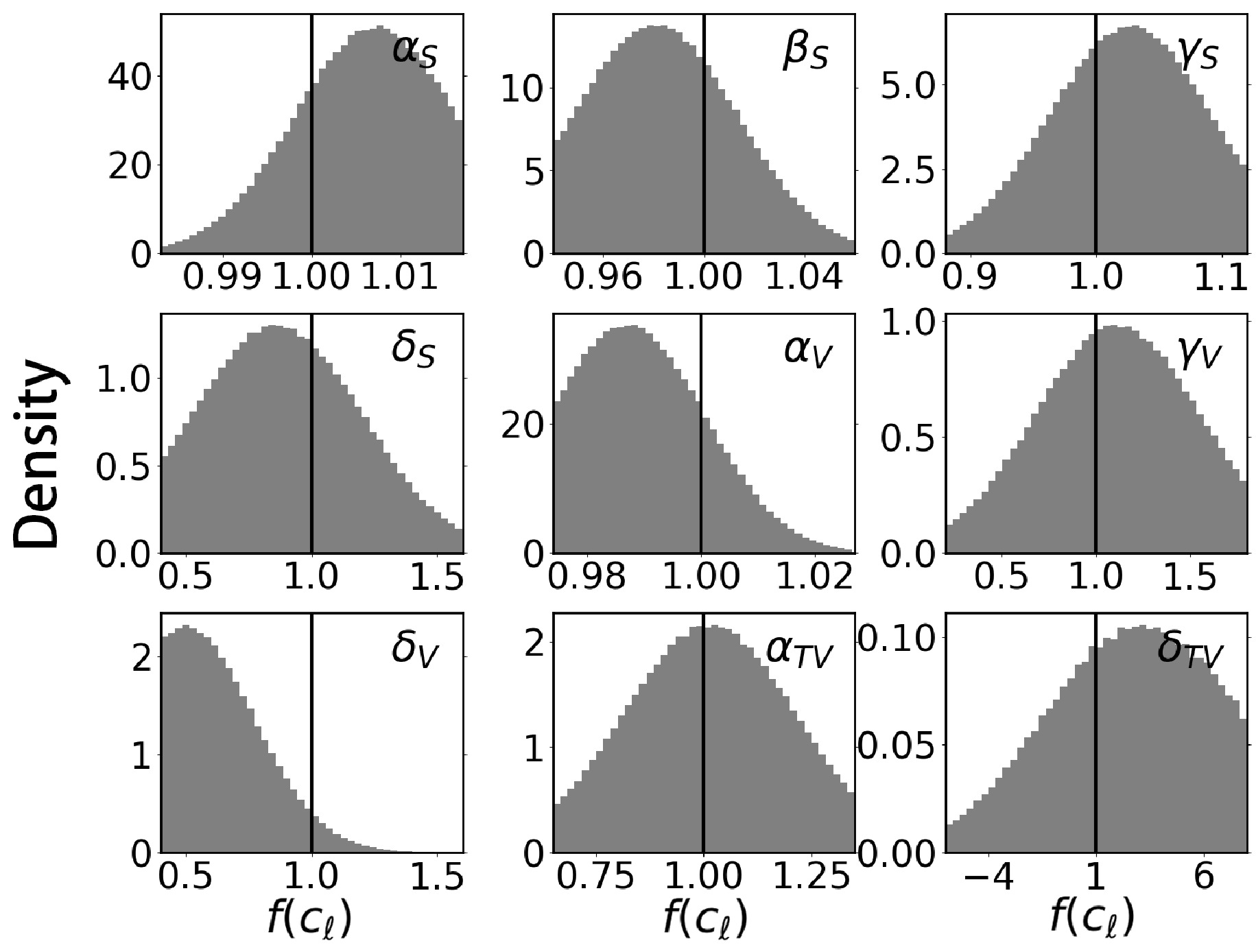
Figure 8. The posterior distributions
$ p({\bf{C}}|{\cal{D}}) $ , defined in (42), are shown for the nine parameters (normalized to PC-PK1) of the relativistic EDF from the Bayesian analysis. The data$ {\cal{D}} $ comprise the empirical values of nuclear matter at saturation density$ {\bf{\Theta}}_{\rm sat} $ , the properties of nuclear matter below saturation density$ {\bf{\Theta}}_{\rm low} $ from the chiral nuclear force, and the$ B(E2;0_1^+\to 2_1^+) $ data for$ ^{136} {\rm{Xe}}$ .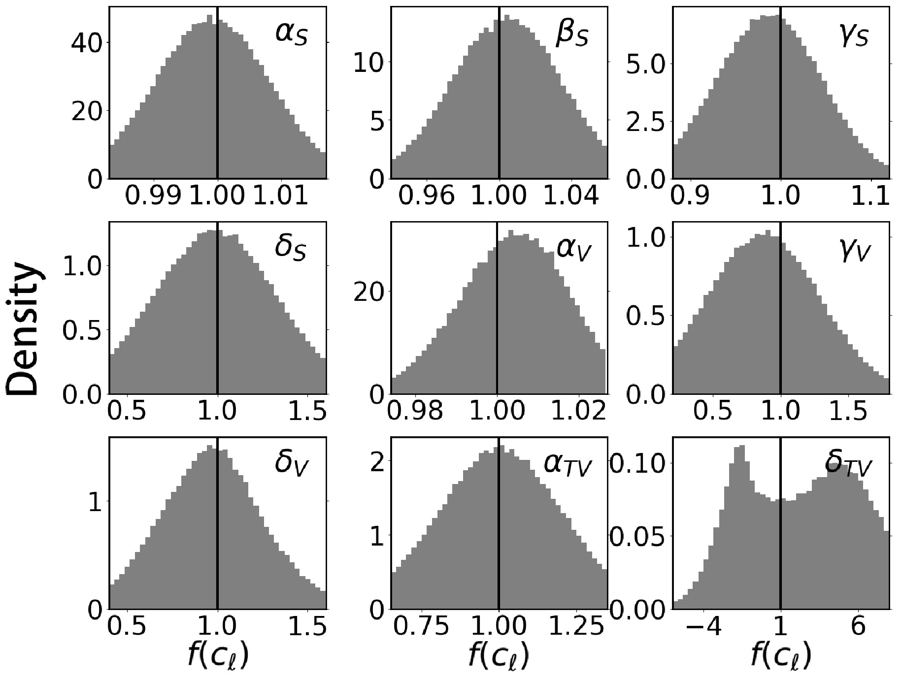
Figure 9. Same as Fig. 8, but with the
$ B(E2:0_1^+\to 2_1^+) $ data for$ ^{136} {\rm{Xe}}$ replaced by the corresponding data for 150Nd.The main peaks of the posterior distribution
$ p({\boldsymbol{C}}|{\cal{D}}) $ for most parameters derived from the$ B(E2) $ data of$ ^{136} {\rm{Xe}}$ are offset from their PC-PK1 values. In contrast, the parameters derived from the$ B(E2) $ data of$ ^{150} {\rm{Nd}}$ align well with the PC-PK1 values. This difference can be understood from the observation that the$ B(E2) $ of$ ^{150} {\rm{Nd}}$ is much better described with the present MR-CDFT than that of$ ^{136} {\rm{Xe}}$ , as detailed in Table 3. The table lists the median and uncertainties of the posteriors for the excitation energies of the$ 2^+_1 $ and$ 4^+_1 $ states and$ E2 $ transition strengths in the four nuclei. The posterior distribution of the observables in Eq. (41) is obtained by incorporating the experimental$ B(E2;0_1^+\to 2_1^+) $ values for each isotope into the determination of the posterior distribution of the EDF parameters in Eq. (42). The excitation energies of the deformed nuclei 150Nd and 150Sm are excellently reproduced, whereas those of the near-spherical nuclei 136Xe and 136Ba are overestimated. The ratio$ R_{42}=E_x(4^+_1)/E_x(2^+_1)<2 $ in both 136Xe and 136Ba indicates that their$ 2^+_1 $ and$ 4^+_1 $ states are dominated by seniority coupling [95], the description of which requires the inclusion of non-collective excitation configurations [84]. The weak collective nature of the$ 2^+_1 $ and$ 4^+_1 $ states in 136Xe and 136Ba can also be inferred from the weak$ E2 $ transition strengths. With the posterior distribution, we finally derive the statistical uncertainties for the low-lying states, which are generally within 21% for excitation energies and 12% for$ E2 $ transition strengths.$ E_x(2^+_1) $ $ E_x(4^+_1) $ $ B(E2:2^+_1\to 4^+_1) $ $ B(E2:0^+_1\to 2^+_1) $ $ ^{150} {\rm{Nd}}$ Exp. 0.130 0.381 1.539(14) 2.745(70) Calc. $ 0.146^{+0.022}_{-0.027} $ $ 0.461^{+0.057}_{-0.068} $ $ 1.579^{+0.131}_{-0.101} $ $ 2.918^{+0.309}_{-0.250} $ $ ^{150} {\rm{Sm}}$ Exp. 0.334 0.773 0.937(145) 1.351(31) Calc. $ 0.301^{+0.041}_{-0.062} $ $ 0.789^{+0.059}_{-0.094} $ $ 1.112^{+0.081}_{-0.054} $ $ 1.913^{+0.226}_{-0.134} $ $ ^{136} {\rm{Xe}}$ Exp. 1.313 1.694 0.0096(1) 0.217(33) Calc. $ 2.872^{+0.069}_{-0.072} $ $ 5.864^{+0.117}_{-0.129} $ $ 0.224^{+0.004}_{-0.004} $ $ 0.364^{+0.008}_{-0.009} $ $ ^{136} {\rm{Ba}}$ Exp. 0.819 1.551 0.119(51) 0.464(9) Calc. $ 1.756^{+0.065}_{-0.086} $ $ 3.548^{+0.195}_{-0.200} $ $ 0.278^{+0.019}_{-0.018} $ $ 0.451^{+0.020}_{-0.021} $ Table 3. The excitation energies (in MeV) of the
$ 2^+_1 $ and$ 4^+_1 $ states and the$ E2 $ transition strengths (in e$ ^2 $ b$ ^2 $ ) are derived from the posteriors of the SP-CDFT calculations for 150Nd, 150Sm, 136Xe, and 136Ba. The results are compared with available data [92]. For the theoretical results, the median, 4th percentile, and 96th percentile of the values are provided. -
Using the above non-implausible samples, we calculated the physical quantities of low-lying nuclear states with SP-CDFT(14,
$ k_{\rm max} $ ) for 150Nd, 150Sm, 136Xe, and 136Ba. The results for 136Xe and 150Nd, with and without refinement from nuclear matter properties, are shown in red and blue in Fig. 6. Because the results for 150Sm closely resemble those for 150Nd, and those for 136Ba are similar to 136Xe, we do not display them here. As shown in the figure, the ground-state energy is only weakly correlated with the excitation energies of the$ 2^+_1 $ and$ 4^+_1 $ states, as well as with the corresponding$ E2 $ transition strengths, and this weak correlation appears to be nucleus-dependent. In contrast, the ground-state energy (or equivalently, the binding energy with the opposite sign) is strongly positively (or negatively) correlated with the proton rms radius in both spherical and deformed nuclei. This suggests that the correlation is not primarily driven by deformation, but rather by changes in the nuclear-matter equation of state (EOS): parameter sets that yield larger ground-state binding energies tend to correspond to larger saturation densities$ \rho_0 $ and smaller proton rms radii$ R_p $ , as shown in Ref. [60].
Figure 6. (color online) Correlations between different quantities of low-lying states. The diagonal panels show histograms of the probability distributions of these quantities for (a) 136Xe and (b) 150Nd. The red distributions are refined by the empirical values of the physical quantities
$ \Theta_{\rm sat}=\{\rho_0, E/A, E_{\rm sym}, L, K\} $ for infinite nuclear matter at saturation density using the$ \sqrt{3}\sigma $ rule. The black circles denote experimental values taken from [92]. See the main text for details.Moreover, the excitation energies of the
$ 2^+_1 $ and$ 4^+_1 $ states and the corresponding$ E2 $ transition strengths among them are governed by quadrupole deformation. Figure 6 clearly shows that the excitation energies and$ B(E2) $ values are strongly anticorrelated with each other in both nuclei, confirming that these correlations are dominated by the deformation effect. This correlation is stronger in the deformed nucleus 150Nd than in 136Xe. In particular, the proton radius$ R_p $ of the ground state is positively correlated with$ B(E2: 0^+_1 \to 2^+_1) $ in 136Xe, whereas it is anticorrelated in 150Nd. This further confirms that the variation of$ R_p $ is not dominated by quadrupole deformation, but by changes in the EOS.To understand the anticorrelation in 150Nd, we plot the unnormalized mean-squared radii
$ \bar{R}_p^2 $ against the unnormalized reduced$ E2 $ transition matrix element$ |\bar{Q}_p| $ from single-configuration calculations using different EDF parameter sets in Fig. 7. These quantities are strongly positively correlated, as expected. Because the normalization factor$ \sqrt{N_0} $ of the$ J=0 $ state is linearly correlated with the normalization factor$ \sqrt{N_2} $ of the$ J=2 $ state with a nonzero intercept, an anticorrelation arises between the normalized mean-squared radii$ R_p^2 $ and the normalized reduced$ E2 $ transition matrix element$ |Q_p| $ , as illustrated in Fig. 7(c). This anticorrelation persists in the configuration-mixing GCM calculation, as shown in Fig. 7(d). In short,$ B(E2: 0^+_1 \to 2^+_1) $ can be either positively or negatively correlated with the proton radius$ R_p $ of the ground state.
Figure 7. (a), (b), (c) Correlations among the mean-squared radius
$ R_p^2=N^{-1}_0\left\langle {J=0NZ;\beta_2,{\bf{C}}}\right|\hat R^2_p\left| {J=0NZ;\beta_2,{\bf{C}}}\right\rangle $ , the reduced$ E2 $ transition matrix element$ Q_p=(N_0N_2)^{-1/2}\left\langle J=2NZ;\beta_2, \right. $ $ \left. {\bf{C}}\right||\hat Q_2|\left| {J=0NZ;\beta_2,{\bf{C}}}\right\rangle $ , and the normalization factors$ \sqrt{N_{J}} $ from calculations for 150Nd based on a single configuration with$ \beta_2=0.3 $ , where$ N_J=\left\langle {JNZ;\beta_2,{\bf{C}}}\right|JNZ;\beta_2,{\bf{C}}\rangle $ . (d) Results from configuration-mixing MR-CDFT calculations. The quantities denoted with bars are unnormalized.Subsequently, we use the Bayesian method to derive the posterior distribution
$ p({\cal{O}}|{\cal{D}}) $ for the quantity$ {\cal{O}} $ given the data$ {\cal{D}} $ . The true value$ {\cal{O}}^{(\rm{true})} $ of$ {\cal{O}} $ can be decomposed as follows [93],$ {\cal{O}}^{(\rm{true})} ={\cal{O}}^{(\rm{MR-CDFT})}({\boldsymbol{C}}) +\delta^{(\rm{syst})}, $
(38) where the systematic uncertainty
$ \delta^{(\rm{syst})} $ includes errors associated with the choice of the particular EDF in Eq. (1), as well as those arising from the truncation of the model space in the present implementation of MR-CDFT, such as the omission of quasiparticle excitations and other collective degrees of freedom. Because$ \delta^{(\rm{syst})} $ is difficult to quantify within the EDF framework, we focus here on the statistical uncertainty of the present MR-CDFT. The quantity$ {\cal{O}}^{(\rm{MR-CDFT})}({\boldsymbol{C}}) $ denotes the value obtained from MR-CDFT based on the parameter set C, and it is further decomposed into two terms in this work,$ {\cal{O}}^{(\rm{MR-CDFT})} ({\boldsymbol{C}})={\cal{O}}^{(\rm{SP-CDFT})}({\boldsymbol{C}})+\delta^{(\rm{em})}. $
(39) Both the systematic error and the emulator error are assumed to follow normal distributions
$ \delta^{\mathrm{(em)}} \sim {\cal{N}}(0, \sigma_{(\mathrm{em})}), $
(40) and are treated as independent.
This posterior distribution can be expressed as an integral incorporating statistical information from various parameter sets:
$ p({\cal{O}}|{\cal{D}})=\int p({\cal{O}}|{\boldsymbol{C}}) p({\boldsymbol{C}}|{\cal{D}}) {\mathrm{d}}{\boldsymbol{C}}, $
(41) where
$ p({\boldsymbol{C}}|{\cal{D}}) $ denotes the posterior distribution of the model parameters C and is obtained via Bayes' theorem:$ p({\boldsymbol{C}}|{\cal{D}})=\dfrac{p({\cal{D}}|{\boldsymbol{C}}) \pi({\boldsymbol{C}})}{p({\cal{D}})}. $
(42) In this equation,
$ p({\cal{D}}) $ serves as a normalization constant. The prior distribution of the parameters,$ \pi({\boldsymbol{C}}) $ , reflects the empirical evaluation of each parameter set C. Here, we assume that the prior distribution follows an uncorrelated multivariate normal distribution,$ \pi({\rm C}) \propto \exp(-\chi_0^2/2),\quad \chi_0^2=\sum\limits_{\ell=1}^{9}\dfrac{(c_\ell-c_\ell^0)^2}{\sigma_\ell^2}, $
(43) where
$ c_\ell^0 $ is the value of the ℓ-th parameter in the PC-PK1 set, and$ \sigma_\ell $ is the standard deviation of the parameter$ c_\ell $ in the samples from the quasi-MC sampling method mentioned previously.Following the Gaussian model [94], the likelihood function
$ p({\cal{D}}|{\boldsymbol{C}}) $ also takes the$ \begin{array}{l} \ \ \ \ \ p( {\cal{D}}|{\boldsymbol{C}}) \\ \propto \exp\left[-\dfrac{1}{2}\Bigg({\boldsymbol{D}}^{\rm (em)}({ {\boldsymbol{C}}})-{\boldsymbol{D}}^{\rm (exp)}\Bigg)^T \Sigma^{-1}\Bigg({\boldsymbol{D}}^{\rm (em)}({ {\boldsymbol{C}}})-{\boldsymbol{D}}^{\rm (exp)}\Bigg)\right], \end{array}$
(44) where
$ {\boldsymbol{D}}^{\rm (em)}({ {\boldsymbol{C}}}) $ denotes the values of a set of quantities predicted by the emulator based on the parameter set C, and$ {\boldsymbol{D}}^{\rm (exp)} $ represents the corresponding data or empirical values. The resulting$ p({\cal{D}}|{\boldsymbol{C}}) $ for the quantities$ {\cal{D}} $ is used to constrain the parameter C via the Bayesian method.The covariance matrix
$ \Sigma_{ij} $ is obtained from the Pearson correlation coefficient$ \rho_{ij} $ as$ \Sigma_{ij}=\sigma_i\rho_{ij} \sigma_j $ , where$ \sigma_{i} $ denotes the standard deviation of the SP-CDFT calculation for the i-th quantity relative to the corresponding data or empirical value. The Pearson correlation coefficient$ \rho_{ij} $ is defined in terms of expectation values as$ \rho_{ij}= \dfrac{\mathbb{E}\big[(D_i-\mu_i)(D_j-\mu_j)\big]} {\sqrt{\mathbb{E}[(D_i-\mu_i)^2]}\,\sqrt{\mathbb{E}[(D_j-\mu_j)^2]}}, $
(45) where
$ \mu_i $ is the mean value of the i-th quantity. The covariance matrix encapsulates the correlation between the i-th and j-th quantities.The predictive distribution
$ p({\cal{O}}|{\boldsymbol{C}}) $ in Eq. (41) is given by$ p({\cal{O}}|{\boldsymbol{C}})=\int p({\cal{O}}|{\boldsymbol{C}};\sigma_{\rm{(MR)}})p(\sigma_{\rm{(MR)}}){\mathrm{d}}\sigma_{\rm{(MR)}}. $
(46) Under the Gaussian model, if the prior for the systematic error
$ p(\sigma_{\rm{(MR)}}) $ is taken as a delta function at$ \sigma_{\rm{0}} $ , the predictive distribution simplifies to$ p({\cal{O}}|{\boldsymbol{C}}) \propto \exp\Bigg\{-\dfrac{[{\cal{O}}-{\cal{O}}^{\rm (em)}({\boldsymbol{C}})]^2}{2(\sigma_{(\rm{em})}^2+\sigma_{0}^2)}\Bigg\}, $
(47) where
$ {\cal{O}}^{\rm (em)}({\boldsymbol{C}}) $ is the emulator prediction for the quantity$ {\cal{O}} $ using the parameter set C, and$ \sigma_{\rm{(em)}} $ is the emulator uncertainty for this quantity. In this work,$ \sigma_{0} $ is determined from the deviation between the current MR-CDFT predictions using PC-PK1 and the experimental data for the quantities considered.Since the original optimization of the EDF parameters C in PC-PK1 did not include low-lying collective observables, the resulting prior distribution is not necessarily optimal for describing spectroscopic properties. We therefore use the experimental
$ B(E2;0_1^+\to 2_1^+) $ values to re-weight the sampled EDF parameters, thereby deriving an empirical distribution better constrained by collective quadrupole correlations and suitable for quantifying the corresponding uncertainties. Figure 8 shows the posterior distribution$ p({\boldsymbol{C}}|{\cal{D}}) $ of each parameter$ c_\ell $ , where the data$ {\cal{D}} $ contain the empirical values of the nuclear-matter properties$ {\boldsymbol{\Theta}}_{\rm sat} $ at saturation density, those below saturation density$ {\boldsymbol{\Theta}}_{\rm low} $ obtained from many-body perturbation theory calculations based on a chiral$ NN+3N $ potential up to N3LO [90], and the$ B(E2;0_1^+\to 2_1^+) $ data for$ ^{136} {\rm{Xe}}$ . Figure 9 shows the posterior distribution$ p({\boldsymbol{C}}|{\cal{D}}) $ , which is obtained similarly to Fig. 8 but with the$ B(E2;0_1^+ \to 2_1^+) $ of$ ^{136} {\rm{Xe}}$ replaced by that of$ ^{150} {\rm{Nd}}$ .
Figure 8. The posterior distributions
$ p({\bf{C}}|{\cal{D}}) $ , defined in (42), are shown for the nine parameters (normalized to PC-PK1) of the relativistic EDF from the Bayesian analysis. The data$ {\cal{D}} $ comprise the empirical values of nuclear matter at saturation density$ {\bf{\Theta}}_{\rm sat} $ , the properties of nuclear matter below saturation density$ {\bf{\Theta}}_{\rm low} $ from the chiral nuclear force, and the$ B(E2;0_1^+\to 2_1^+) $ data for$ ^{136} {\rm{Xe}}$ .
Figure 9. Same as Fig. 8, but with the
$ B(E2:0_1^+\to 2_1^+) $ data for$ ^{136} {\rm{Xe}}$ replaced by the corresponding data for 150Nd.The main peaks of the posterior distribution
$ p({\boldsymbol{C}}|{\cal{D}}) $ for most parameters derived from the$ B(E2) $ data of$ ^{136} {\rm{Xe}}$ are offset from their PC-PK1 values. In contrast, the parameters derived from the$ B(E2) $ data of$ ^{150} {\rm{Nd}}$ align well with the PC-PK1 values. This difference can be understood from the observation that the$ B(E2) $ of$ ^{150} {\rm{Nd}}$ is much better described with the present MR-CDFT than that of$ ^{136} {\rm{Xe}}$ , as detailed in Table 3. The table lists the median and uncertainties of the posteriors for the excitation energies of the$ 2^+_1 $ and$ 4^+_1 $ states and$ E2 $ transition strengths in the four nuclei. The posterior distribution of the observables in Eq. (41) is obtained by incorporating the experimental$ B(E2;0_1^+\to 2_1^+) $ values for each isotope into the determination of the posterior distribution of the EDF parameters in Eq. (42). The excitation energies of the deformed nuclei 150Nd and 150Sm are excellently reproduced, whereas those of the near-spherical nuclei 136Xe and 136Ba are overestimated. The ratio$ R_{42}=E_x(4^+_1)/E_x(2^+_1)<2 $ in both 136Xe and 136Ba indicates that their$ 2^+_1 $ and$ 4^+_1 $ states are dominated by seniority coupling [95], the description of which requires the inclusion of non-collective excitation configurations [84]. The weak collective nature of the$ 2^+_1 $ and$ 4^+_1 $ states in 136Xe and 136Ba can also be inferred from the weak$ E2 $ transition strengths. With the posterior distribution, we finally derive the statistical uncertainties for the low-lying states, which are generally within 21% for excitation energies and 12% for$ E2 $ transition strengths.$ E_x(2^+_1) $ $ E_x(4^+_1) $ $ B(E2:2^+_1\to 4^+_1) $ $ B(E2:0^+_1\to 2^+_1) $ $ ^{150} {\rm{Nd}}$ Exp. 0.130 0.381 1.539(14) 2.745(70) Calc. $ 0.146^{+0.022}_{-0.027} $ $ 0.461^{+0.057}_{-0.068} $ $ 1.579^{+0.131}_{-0.101} $ $ 2.918^{+0.309}_{-0.250} $ $ ^{150} {\rm{Sm}}$ Exp. 0.334 0.773 0.937(145) 1.351(31) Calc. $ 0.301^{+0.041}_{-0.062} $ $ 0.789^{+0.059}_{-0.094} $ $ 1.112^{+0.081}_{-0.054} $ $ 1.913^{+0.226}_{-0.134} $ $ ^{136} {\rm{Xe}}$ Exp. 1.313 1.694 0.0096(1) 0.217(33) Calc. $ 2.872^{+0.069}_{-0.072} $ $ 5.864^{+0.117}_{-0.129} $ $ 0.224^{+0.004}_{-0.004} $ $ 0.364^{+0.008}_{-0.009} $ $ ^{136} {\rm{Ba}}$ Exp. 0.819 1.551 0.119(51) 0.464(9) Calc. $ 1.756^{+0.065}_{-0.086} $ $ 3.548^{+0.195}_{-0.200} $ $ 0.278^{+0.019}_{-0.018} $ $ 0.451^{+0.020}_{-0.021} $ Table 3. The excitation energies (in MeV) of the
$ 2^+_1 $ and$ 4^+_1 $ states and the$ E2 $ transition strengths (in e$ ^2 $ b$ ^2 $ ) are derived from the posteriors of the SP-CDFT calculations for 150Nd, 150Sm, 136Xe, and 136Ba. The results are compared with available data [92]. For the theoretical results, the median, 4th percentile, and 96th percentile of the values are provided. -
Using the above non-implausible samples, we calculated the physical quantities of low-lying nuclear states with SP-CDFT(14,
$ k_{\rm max} $ ) for 150Nd, 150Sm, 136Xe, and 136Ba. The results for 136Xe and 150Nd, with and without refinement from nuclear matter properties, are shown in red and blue in Fig. 6. Because the results for 150Sm closely resemble those for 150Nd, and those for 136Ba are similar to 136Xe, we do not display them here. As shown in the figure, the ground-state energy is only weakly correlated with the excitation energies of the$ 2^+_1 $ and$ 4^+_1 $ states, as well as with the corresponding$ E2 $ transition strengths, and this weak correlation appears to be nucleus-dependent. In contrast, the ground-state energy (or equivalently, the binding energy with the opposite sign) is strongly positively (or negatively) correlated with the proton rms radius in both spherical and deformed nuclei. This suggests that the correlation is not primarily driven by deformation, but rather by changes in the nuclear-matter equation of state (EOS): parameter sets that yield larger ground-state binding energies tend to correspond to larger saturation densities$ \rho_0 $ and smaller proton rms radii$ R_p $ , as shown in Ref. [60].
Figure 6. (color online) Correlations between different quantities of low-lying states. The diagonal panels show histograms of the probability distributions of these quantities for (a) 136Xe and (b) 150Nd. The red distributions are refined by the empirical values of the physical quantities
$ \Theta_{\rm sat}=\{\rho_0, E/A, E_{\rm sym}, L, K\} $ for infinite nuclear matter at saturation density using the$ \sqrt{3}\sigma $ rule. The black circles denote experimental values taken from [92]. See the main text for details.Moreover, the excitation energies of the
$ 2^+_1 $ and$ 4^+_1 $ states and the corresponding$ E2 $ transition strengths among them are governed by quadrupole deformation. Figure 6 clearly shows that the excitation energies and$ B(E2) $ values are strongly anticorrelated with each other in both nuclei, confirming that these correlations are dominated by the deformation effect. This correlation is stronger in the deformed nucleus 150Nd than in 136Xe. In particular, the proton radius$ R_p $ of the ground state is positively correlated with$ B(E2: 0^+_1 \to 2^+_1) $ in 136Xe, whereas it is anticorrelated in 150Nd. This further confirms that the variation of$ R_p $ is not dominated by quadrupole deformation, but by changes in the EOS.To understand the anticorrelation in 150Nd, we plot the unnormalized mean-squared radii
$ \bar{R}_p^2 $ against the unnormalized reduced$ E2 $ transition matrix element$ |\bar{Q}_p| $ from single-configuration calculations using different EDF parameter sets in Fig. 7. These quantities are strongly positively correlated, as expected. Because the normalization factor$ \sqrt{N_0} $ of the$ J=0 $ state is linearly correlated with the normalization factor$ \sqrt{N_2} $ of the$ J=2 $ state with a nonzero intercept, an anticorrelation arises between the normalized mean-squared radii$ R_p^2 $ and the normalized reduced$ E2 $ transition matrix element$ |Q_p| $ , as illustrated in Fig. 7(c). This anticorrelation persists in the configuration-mixing GCM calculation, as shown in Fig. 7(d). In short,$ B(E2: 0^+_1 \to 2^+_1) $ can be either positively or negatively correlated with the proton radius$ R_p $ of the ground state.
Figure 7. (a), (b), (c) Correlations among the mean-squared radius
$ R_p^2=N^{-1}_0\left\langle {J=0NZ;\beta_2,{\bf{C}}}\right|\hat R^2_p\left| {J=0NZ;\beta_2,{\bf{C}}}\right\rangle $ , the reduced$ E2 $ transition matrix element$ Q_p=(N_0N_2)^{-1/2}\left\langle J=2NZ;\beta_2, \right. $ $ \left. {\bf{C}}\right||\hat Q_2|\left| {J=0NZ;\beta_2,{\bf{C}}}\right\rangle $ , and the normalization factors$ \sqrt{N_{J}} $ from calculations for 150Nd based on a single configuration with$ \beta_2=0.3 $ , where$ N_J=\left\langle {JNZ;\beta_2,{\bf{C}}}\right|JNZ;\beta_2,{\bf{C}}\rangle $ . (d) Results from configuration-mixing MR-CDFT calculations. The quantities denoted with bars are unnormalized.Subsequently, we use the Bayesian method to derive the posterior distribution
$ p({\cal{O}}|{\cal{D}}) $ for the quantity$ {\cal{O}} $ given the data$ {\cal{D}} $ . The true value$ {\cal{O}}^{(\rm{true})} $ of$ {\cal{O}} $ can be decomposed as follows [93],$ {\cal{O}}^{(\rm{true})} ={\cal{O}}^{(\rm{MR-CDFT})}({\boldsymbol{C}}) +\delta^{(\rm{syst})}, $
(38) where the systematic uncertainty
$ \delta^{(\rm{syst})} $ includes errors associated with the choice of the particular EDF in Eq. (1), as well as those arising from the truncation of the model space in the present implementation of MR-CDFT, such as the omission of quasiparticle excitations and other collective degrees of freedom. Because$ \delta^{(\rm{syst})} $ is difficult to quantify within the EDF framework, we focus here on the statistical uncertainty of the present MR-CDFT. The quantity$ {\cal{O}}^{(\rm{MR-CDFT})}({\boldsymbol{C}}) $ denotes the value obtained from MR-CDFT based on the parameter set C, and it is further decomposed into two terms in this work,$ {\cal{O}}^{(\rm{MR-CDFT})} ({\boldsymbol{C}})={\cal{O}}^{(\rm{SP-CDFT})}({\boldsymbol{C}})+\delta^{(\rm{em})}. $
(39) Both the systematic error and the emulator error are assumed to follow normal distributions
$ \delta^{\mathrm{(em)}} \sim {\cal{N}}(0, \sigma_{(\mathrm{em})}), $
(40) and are treated as independent.
This posterior distribution can be expressed as an integral incorporating statistical information from various parameter sets:
$ p({\cal{O}}|{\cal{D}})=\int p({\cal{O}}|{\boldsymbol{C}}) p({\boldsymbol{C}}|{\cal{D}}) {\mathrm{d}}{\boldsymbol{C}}, $
(41) where
$ p({\boldsymbol{C}}|{\cal{D}}) $ denotes the posterior distribution of the model parameters C and is obtained via Bayes' theorem:$ p({\boldsymbol{C}}|{\cal{D}})=\dfrac{p({\cal{D}}|{\boldsymbol{C}}) \pi({\boldsymbol{C}})}{p({\cal{D}})}. $
(42) In this equation,
$ p({\cal{D}}) $ serves as a normalization constant. The prior distribution of the parameters,$ \pi({\boldsymbol{C}}) $ , reflects the empirical evaluation of each parameter set C. Here, we assume that the prior distribution follows an uncorrelated multivariate normal distribution,$ \pi({\rm C}) \propto \exp(-\chi_0^2/2),\quad \chi_0^2=\sum\limits_{\ell=1}^{9}\dfrac{(c_\ell-c_\ell^0)^2}{\sigma_\ell^2}, $
(43) where
$ c_\ell^0 $ is the value of the ℓ-th parameter in the PC-PK1 set, and$ \sigma_\ell $ is the standard deviation of the parameter$ c_\ell $ in the samples from the quasi-MC sampling method mentioned previously.Following the Gaussian model [94], the likelihood function
$ p({\cal{D}}|{\boldsymbol{C}}) $ also takes the$ \begin{array}{l} \ \ \ \ \ p( {\cal{D}}|{\boldsymbol{C}}) \\ \propto \exp\left[-\dfrac{1}{2}\Bigg({\boldsymbol{D}}^{\rm (em)}({ {\boldsymbol{C}}})-{\boldsymbol{D}}^{\rm (exp)}\Bigg)^T \Sigma^{-1}\Bigg({\boldsymbol{D}}^{\rm (em)}({ {\boldsymbol{C}}})-{\boldsymbol{D}}^{\rm (exp)}\Bigg)\right], \end{array}$
(44) where
$ {\boldsymbol{D}}^{\rm (em)}({ {\boldsymbol{C}}}) $ denotes the values of a set of quantities predicted by the emulator based on the parameter set C, and$ {\boldsymbol{D}}^{\rm (exp)} $ represents the corresponding data or empirical values. The resulting$ p({\cal{D}}|{\boldsymbol{C}}) $ for the quantities$ {\cal{D}} $ is used to constrain the parameter C via the Bayesian method.The covariance matrix
$ \Sigma_{ij} $ is obtained from the Pearson correlation coefficient$ \rho_{ij} $ as$ \Sigma_{ij}=\sigma_i\rho_{ij} \sigma_j $ , where$ \sigma_{i} $ denotes the standard deviation of the SP-CDFT calculation for the i-th quantity relative to the corresponding data or empirical value. The Pearson correlation coefficient$ \rho_{ij} $ is defined in terms of expectation values as$ \rho_{ij}= \dfrac{\mathbb{E}\big[(D_i-\mu_i)(D_j-\mu_j)\big]} {\sqrt{\mathbb{E}[(D_i-\mu_i)^2]}\,\sqrt{\mathbb{E}[(D_j-\mu_j)^2]}}, $
(45) where
$ \mu_i $ is the mean value of the i-th quantity. The covariance matrix encapsulates the correlation between the i-th and j-th quantities.The predictive distribution
$ p({\cal{O}}|{\boldsymbol{C}}) $ in Eq. (41) is given by$ p({\cal{O}}|{\boldsymbol{C}})=\int p({\cal{O}}|{\boldsymbol{C}};\sigma_{\rm{(MR)}})p(\sigma_{\rm{(MR)}}){\mathrm{d}}\sigma_{\rm{(MR)}}. $
(46) Under the Gaussian model, if the prior for the systematic error
$ p(\sigma_{\rm{(MR)}}) $ is taken as a delta function at$ \sigma_{\rm{0}} $ , the predictive distribution simplifies to$ p({\cal{O}}|{\boldsymbol{C}}) \propto \exp\Bigg\{-\dfrac{[{\cal{O}}-{\cal{O}}^{\rm (em)}({\boldsymbol{C}})]^2}{2(\sigma_{(\rm{em})}^2+\sigma_{0}^2)}\Bigg\}, $
(47) where
$ {\cal{O}}^{\rm (em)}({\boldsymbol{C}}) $ is the emulator prediction for the quantity$ {\cal{O}} $ using the parameter set C, and$ \sigma_{\rm{(em)}} $ is the emulator uncertainty for this quantity. In this work,$ \sigma_{0} $ is determined from the deviation between the current MR-CDFT predictions using PC-PK1 and the experimental data for the quantities considered.Since the original optimization of the EDF parameters C in PC-PK1 did not include low-lying collective observables, the resulting prior distribution is not necessarily optimal for describing spectroscopic properties. We therefore use the experimental
$ B(E2;0_1^+\to 2_1^+) $ values to re-weight the sampled EDF parameters, thereby deriving an empirical distribution better constrained by collective quadrupole correlations and suitable for quantifying the corresponding uncertainties. Figure 8 shows the posterior distribution$ p({\boldsymbol{C}}|{\cal{D}}) $ of each parameter$ c_\ell $ , where the data$ {\cal{D}} $ contain the empirical values of the nuclear-matter properties$ {\boldsymbol{\Theta}}_{\rm sat} $ at saturation density, those below saturation density$ {\boldsymbol{\Theta}}_{\rm low} $ obtained from many-body perturbation theory calculations based on a chiral$ NN+3N $ potential up to N3LO [90], and the$ B(E2;0_1^+\to 2_1^+) $ data for$ ^{136} {\rm{Xe}}$ . Figure 9 shows the posterior distribution$ p({\boldsymbol{C}}|{\cal{D}}) $ , which is obtained similarly to Fig. 8 but with the$ B(E2;0_1^+ \to 2_1^+) $ of$ ^{136} {\rm{Xe}}$ replaced by that of$ ^{150} {\rm{Nd}}$ .
Figure 8. The posterior distributions
$ p({\bf{C}}|{\cal{D}}) $ , defined in (42), are shown for the nine parameters (normalized to PC-PK1) of the relativistic EDF from the Bayesian analysis. The data$ {\cal{D}} $ comprise the empirical values of nuclear matter at saturation density$ {\bf{\Theta}}_{\rm sat} $ , the properties of nuclear matter below saturation density$ {\bf{\Theta}}_{\rm low} $ from the chiral nuclear force, and the$ B(E2;0_1^+\to 2_1^+) $ data for$ ^{136} {\rm{Xe}}$ .
Figure 9. Same as Fig. 8, but with the
$ B(E2:0_1^+\to 2_1^+) $ data for$ ^{136} {\rm{Xe}}$ replaced by the corresponding data for 150Nd.The main peaks of the posterior distribution
$ p({\boldsymbol{C}}|{\cal{D}}) $ for most parameters derived from the$ B(E2) $ data of$ ^{136} {\rm{Xe}}$ are offset from their PC-PK1 values. In contrast, the parameters derived from the$ B(E2) $ data of$ ^{150} {\rm{Nd}}$ align well with the PC-PK1 values. This difference can be understood from the observation that the$ B(E2) $ of$ ^{150} {\rm{Nd}}$ is much better described with the present MR-CDFT than that of$ ^{136} {\rm{Xe}}$ , as detailed in Table 3. The table lists the median and uncertainties of the posteriors for the excitation energies of the$ 2^+_1 $ and$ 4^+_1 $ states and$ E2 $ transition strengths in the four nuclei. The posterior distribution of the observables in Eq. (41) is obtained by incorporating the experimental$ B(E2;0_1^+\to 2_1^+) $ values for each isotope into the determination of the posterior distribution of the EDF parameters in Eq. (42). The excitation energies of the deformed nuclei 150Nd and 150Sm are excellently reproduced, whereas those of the near-spherical nuclei 136Xe and 136Ba are overestimated. The ratio$ R_{42}=E_x(4^+_1)/E_x(2^+_1)<2 $ in both 136Xe and 136Ba indicates that their$ 2^+_1 $ and$ 4^+_1 $ states are dominated by seniority coupling [95], the description of which requires the inclusion of non-collective excitation configurations [84]. The weak collective nature of the$ 2^+_1 $ and$ 4^+_1 $ states in 136Xe and 136Ba can also be inferred from the weak$ E2 $ transition strengths. With the posterior distribution, we finally derive the statistical uncertainties for the low-lying states, which are generally within 21% for excitation energies and 12% for$ E2 $ transition strengths.$ E_x(2^+_1) $ $ E_x(4^+_1) $ $ B(E2:2^+_1\to 4^+_1) $ $ B(E2:0^+_1\to 2^+_1) $ $ ^{150} {\rm{Nd}}$ Exp. 0.130 0.381 1.539(14) 2.745(70) Calc. $ 0.146^{+0.022}_{-0.027} $ $ 0.461^{+0.057}_{-0.068} $ $ 1.579^{+0.131}_{-0.101} $ $ 2.918^{+0.309}_{-0.250} $ $ ^{150} {\rm{Sm}}$ Exp. 0.334 0.773 0.937(145) 1.351(31) Calc. $ 0.301^{+0.041}_{-0.062} $ $ 0.789^{+0.059}_{-0.094} $ $ 1.112^{+0.081}_{-0.054} $ $ 1.913^{+0.226}_{-0.134} $ $ ^{136} {\rm{Xe}}$ Exp. 1.313 1.694 0.0096(1) 0.217(33) Calc. $ 2.872^{+0.069}_{-0.072} $ $ 5.864^{+0.117}_{-0.129} $ $ 0.224^{+0.004}_{-0.004} $ $ 0.364^{+0.008}_{-0.009} $ $ ^{136} {\rm{Ba}}$ Exp. 0.819 1.551 0.119(51) 0.464(9) Calc. $ 1.756^{+0.065}_{-0.086} $ $ 3.548^{+0.195}_{-0.200} $ $ 0.278^{+0.019}_{-0.018} $ $ 0.451^{+0.020}_{-0.021} $ Table 3. The excitation energies (in MeV) of the
$ 2^+_1 $ and$ 4^+_1 $ states and the$ E2 $ transition strengths (in e$ ^2 $ b$ ^2 $ ) are derived from the posteriors of the SP-CDFT calculations for 150Nd, 150Sm, 136Xe, and 136Ba. The results are compared with available data [92]. For the theoretical results, the median, 4th percentile, and 96th percentile of the values are provided. -
Using the above non-implausible samples, we calculated the physical quantities of low-lying nuclear states with SP-CDFT(14,
$ k_{\rm max} $ ) for 150Nd, 150Sm, 136Xe, and 136Ba. The results for 136Xe and 150Nd, with and without refinement from nuclear matter properties, are shown in red and blue in Fig. 6. Because the results for 150Sm closely resemble those for 150Nd, and those for 136Ba are similar to 136Xe, we do not display them here. As shown in the figure, the ground-state energy is only weakly correlated with the excitation energies of the$ 2^+_1 $ and$ 4^+_1 $ states, as well as with the corresponding$ E2 $ transition strengths, and this weak correlation appears to be nucleus-dependent. In contrast, the ground-state energy (or equivalently, the binding energy with the opposite sign) is strongly positively (or negatively) correlated with the proton rms radius in both spherical and deformed nuclei. This suggests that the correlation is not primarily driven by deformation, but rather by changes in the nuclear-matter equation of state (EOS): parameter sets that yield larger ground-state binding energies tend to correspond to larger saturation densities$ \rho_0 $ and smaller proton rms radii$ R_p $ , as shown in Ref. [60].
Figure 6. (color online) Correlations between different quantities of low-lying states. The diagonal panels show histograms of the probability distributions of these quantities for (a) 136Xe and (b) 150Nd. The red distributions are refined by the empirical values of the physical quantities
$ \Theta_{\rm sat}=\{\rho_0, E/A, E_{\rm sym}, L, K\} $ for infinite nuclear matter at saturation density using the$ \sqrt{3}\sigma $ rule. The black circles denote experimental values taken from [92]. See the main text for details.Moreover, the excitation energies of the
$ 2^+_1 $ and$ 4^+_1 $ states and the corresponding$ E2 $ transition strengths among them are governed by quadrupole deformation. Figure 6 clearly shows that the excitation energies and$ B(E2) $ values are strongly anticorrelated with each other in both nuclei, confirming that these correlations are dominated by the deformation effect. This correlation is stronger in the deformed nucleus 150Nd than in 136Xe. In particular, the proton radius$ R_p $ of the ground state is positively correlated with$ B(E2: 0^+_1 \to 2^+_1) $ in 136Xe, whereas it is anticorrelated in 150Nd. This further confirms that the variation of$ R_p $ is not dominated by quadrupole deformation, but by changes in the EOS.To understand the anticorrelation in 150Nd, we plot the unnormalized mean-squared radii
$ \bar{R}_p^2 $ against the unnormalized reduced$ E2 $ transition matrix element$ |\bar{Q}_p| $ from single-configuration calculations using different EDF parameter sets in Fig. 7. These quantities are strongly positively correlated, as expected. Because the normalization factor$ \sqrt{N_0} $ of the$ J=0 $ state is linearly correlated with the normalization factor$ \sqrt{N_2} $ of the$ J=2 $ state with a nonzero intercept, an anticorrelation arises between the normalized mean-squared radii$ R_p^2 $ and the normalized reduced$ E2 $ transition matrix element$ |Q_p| $ , as illustrated in Fig. 7(c). This anticorrelation persists in the configuration-mixing GCM calculation, as shown in Fig. 7(d). In short,$ B(E2: 0^+_1 \to 2^+_1) $ can be either positively or negatively correlated with the proton radius$ R_p $ of the ground state.
Figure 7. (a), (b), (c) Correlations among the mean-squared radius
$ R_p^2=N^{-1}_0\left\langle {J=0NZ;\beta_2,{\bf{C}}}\right|\hat R^2_p\left| {J=0NZ;\beta_2,{\bf{C}}}\right\rangle $ , the reduced$ E2 $ transition matrix element$ Q_p=(N_0N_2)^{-1/2}\left\langle J=2NZ;\beta_2, \right. $ $ \left. {\bf{C}}\right||\hat Q_2|\left| {J=0NZ;\beta_2,{\bf{C}}}\right\rangle $ , and the normalization factors$ \sqrt{N_{J}} $ from calculations for 150Nd based on a single configuration with$ \beta_2=0.3 $ , where$ N_J=\left\langle {JNZ;\beta_2,{\bf{C}}}\right|JNZ;\beta_2,{\bf{C}}\rangle $ . (d) Results from configuration-mixing MR-CDFT calculations. The quantities denoted with bars are unnormalized.Subsequently, we use the Bayesian method to derive the posterior distribution
$ p({\cal{O}}|{\cal{D}}) $ for the quantity$ {\cal{O}} $ given the data$ {\cal{D}} $ . The true value$ {\cal{O}}^{(\rm{true})} $ of$ {\cal{O}} $ can be decomposed as follows [93],$ {\cal{O}}^{(\rm{true})} ={\cal{O}}^{(\rm{MR-CDFT})}({\boldsymbol{C}}) +\delta^{(\rm{syst})}, $
(38) where the systematic uncertainty
$ \delta^{(\rm{syst})} $ includes errors associated with the choice of the particular EDF in Eq. (1), as well as those arising from the truncation of the model space in the present implementation of MR-CDFT, such as the omission of quasiparticle excitations and other collective degrees of freedom. Because$ \delta^{(\rm{syst})} $ is difficult to quantify within the EDF framework, we focus here on the statistical uncertainty of the present MR-CDFT. The quantity$ {\cal{O}}^{(\rm{MR-CDFT})}({\boldsymbol{C}}) $ denotes the value obtained from MR-CDFT based on the parameter set C, and it is further decomposed into two terms in this work,$ {\cal{O}}^{(\rm{MR-CDFT})} ({\boldsymbol{C}})={\cal{O}}^{(\rm{SP-CDFT})}({\boldsymbol{C}})+\delta^{(\rm{em})}. $
(39) Both the systematic error and the emulator error are assumed to follow normal distributions
$ \delta^{\mathrm{(em)}} \sim {\cal{N}}(0, \sigma_{(\mathrm{em})}), $
(40) and are treated as independent.
This posterior distribution can be expressed as an integral incorporating statistical information from various parameter sets:
$ p({\cal{O}}|{\cal{D}})=\int p({\cal{O}}|{\boldsymbol{C}}) p({\boldsymbol{C}}|{\cal{D}}) {\mathrm{d}}{\boldsymbol{C}}, $
(41) where
$ p({\boldsymbol{C}}|{\cal{D}}) $ denotes the posterior distribution of the model parameters C and is obtained via Bayes' theorem:$ p({\boldsymbol{C}}|{\cal{D}})=\dfrac{p({\cal{D}}|{\boldsymbol{C}}) \pi({\boldsymbol{C}})}{p({\cal{D}})}. $
(42) In this equation,
$ p({\cal{D}}) $ serves as a normalization constant. The prior distribution of the parameters,$ \pi({\boldsymbol{C}}) $ , reflects the empirical evaluation of each parameter set C. Here, we assume that the prior distribution follows an uncorrelated multivariate normal distribution,$ \pi({\rm C}) \propto \exp(-\chi_0^2/2),\quad \chi_0^2=\sum\limits_{\ell=1}^{9}\dfrac{(c_\ell-c_\ell^0)^2}{\sigma_\ell^2}, $
(43) where
$ c_\ell^0 $ is the value of the ℓ-th parameter in the PC-PK1 set, and$ \sigma_\ell $ is the standard deviation of the parameter$ c_\ell $ in the samples from the quasi-MC sampling method mentioned previously.Following the Gaussian model [94], the likelihood function
$ p({\cal{D}}|{\boldsymbol{C}}) $ also takes the$ \begin{array}{l} \ \ \ \ \ p( {\cal{D}}|{\boldsymbol{C}}) \\ \propto \exp\left[-\dfrac{1}{2}\Bigg({\boldsymbol{D}}^{\rm (em)}({ {\boldsymbol{C}}})-{\boldsymbol{D}}^{\rm (exp)}\Bigg)^T \Sigma^{-1}\Bigg({\boldsymbol{D}}^{\rm (em)}({ {\boldsymbol{C}}})-{\boldsymbol{D}}^{\rm (exp)}\Bigg)\right], \end{array}$
(44) where
$ {\boldsymbol{D}}^{\rm (em)}({ {\boldsymbol{C}}}) $ denotes the values of a set of quantities predicted by the emulator based on the parameter set C, and$ {\boldsymbol{D}}^{\rm (exp)} $ represents the corresponding data or empirical values. The resulting$ p({\cal{D}}|{\boldsymbol{C}}) $ for the quantities$ {\cal{D}} $ is used to constrain the parameter C via the Bayesian method.The covariance matrix
$ \Sigma_{ij} $ is obtained from the Pearson correlation coefficient$ \rho_{ij} $ as$ \Sigma_{ij}=\sigma_i\rho_{ij} \sigma_j $ , where$ \sigma_{i} $ denotes the standard deviation of the SP-CDFT calculation for the i-th quantity relative to the corresponding data or empirical value. The Pearson correlation coefficient$ \rho_{ij} $ is defined in terms of expectation values as$ \rho_{ij}= \dfrac{\mathbb{E}\big[(D_i-\mu_i)(D_j-\mu_j)\big]} {\sqrt{\mathbb{E}[(D_i-\mu_i)^2]}\,\sqrt{\mathbb{E}[(D_j-\mu_j)^2]}}, $
(45) where
$ \mu_i $ is the mean value of the i-th quantity. The covariance matrix encapsulates the correlation between the i-th and j-th quantities.The predictive distribution
$ p({\cal{O}}|{\boldsymbol{C}}) $ in Eq. (41) is given by$ p({\cal{O}}|{\boldsymbol{C}})=\int p({\cal{O}}|{\boldsymbol{C}};\sigma_{\rm{(MR)}})p(\sigma_{\rm{(MR)}}){\mathrm{d}}\sigma_{\rm{(MR)}}. $
(46) Under the Gaussian model, if the prior for the systematic error
$ p(\sigma_{\rm{(MR)}}) $ is taken as a delta function at$ \sigma_{\rm{0}} $ , the predictive distribution simplifies to$ p({\cal{O}}|{\boldsymbol{C}}) \propto \exp\Bigg\{-\dfrac{[{\cal{O}}-{\cal{O}}^{\rm (em)}({\boldsymbol{C}})]^2}{2(\sigma_{(\rm{em})}^2+\sigma_{0}^2)}\Bigg\}, $
(47) where
$ {\cal{O}}^{\rm (em)}({\boldsymbol{C}}) $ is the emulator prediction for the quantity$ {\cal{O}} $ using the parameter set C, and$ \sigma_{\rm{(em)}} $ is the emulator uncertainty for this quantity. In this work,$ \sigma_{0} $ is determined from the deviation between the current MR-CDFT predictions using PC-PK1 and the experimental data for the quantities considered.Since the original optimization of the EDF parameters C in PC-PK1 did not include low-lying collective observables, the resulting prior distribution is not necessarily optimal for describing spectroscopic properties. We therefore use the experimental
$ B(E2;0_1^+\to 2_1^+) $ values to re-weight the sampled EDF parameters, thereby deriving an empirical distribution better constrained by collective quadrupole correlations and suitable for quantifying the corresponding uncertainties. Figure 8 shows the posterior distribution$ p({\boldsymbol{C}}|{\cal{D}}) $ of each parameter$ c_\ell $ , where the data$ {\cal{D}} $ contain the empirical values of the nuclear-matter properties$ {\boldsymbol{\Theta}}_{\rm sat} $ at saturation density, those below saturation density$ {\boldsymbol{\Theta}}_{\rm low} $ obtained from many-body perturbation theory calculations based on a chiral$ NN+3N $ potential up to N3LO [90], and the$ B(E2;0_1^+\to 2_1^+) $ data for$ ^{136} {\rm{Xe}}$ . Figure 9 shows the posterior distribution$ p({\boldsymbol{C}}|{\cal{D}}) $ , which is obtained similarly to Fig. 8 but with the$ B(E2;0_1^+ \to 2_1^+) $ of$ ^{136} {\rm{Xe}}$ replaced by that of$ ^{150} {\rm{Nd}}$ .
Figure 8. The posterior distributions
$ p({\bf{C}}|{\cal{D}}) $ , defined in (42), are shown for the nine parameters (normalized to PC-PK1) of the relativistic EDF from the Bayesian analysis. The data$ {\cal{D}} $ comprise the empirical values of nuclear matter at saturation density$ {\bf{\Theta}}_{\rm sat} $ , the properties of nuclear matter below saturation density$ {\bf{\Theta}}_{\rm low} $ from the chiral nuclear force, and the$ B(E2;0_1^+\to 2_1^+) $ data for$ ^{136} {\rm{Xe}}$ .
Figure 9. Same as Fig. 8, but with the
$ B(E2:0_1^+\to 2_1^+) $ data for$ ^{136} {\rm{Xe}}$ replaced by the corresponding data for 150Nd.The main peaks of the posterior distribution
$ p({\boldsymbol{C}}|{\cal{D}}) $ for most parameters derived from the$ B(E2) $ data of$ ^{136} {\rm{Xe}}$ are offset from their PC-PK1 values. In contrast, the parameters derived from the$ B(E2) $ data of$ ^{150} {\rm{Nd}}$ align well with the PC-PK1 values. This difference can be understood from the observation that the$ B(E2) $ of$ ^{150} {\rm{Nd}}$ is much better described with the present MR-CDFT than that of$ ^{136} {\rm{Xe}}$ , as detailed in Table 3. The table lists the median and uncertainties of the posteriors for the excitation energies of the$ 2^+_1 $ and$ 4^+_1 $ states and$ E2 $ transition strengths in the four nuclei. The posterior distribution of the observables in Eq. (41) is obtained by incorporating the experimental$ B(E2;0_1^+\to 2_1^+) $ values for each isotope into the determination of the posterior distribution of the EDF parameters in Eq. (42). The excitation energies of the deformed nuclei 150Nd and 150Sm are excellently reproduced, whereas those of the near-spherical nuclei 136Xe and 136Ba are overestimated. The ratio$ R_{42}=E_x(4^+_1)/E_x(2^+_1)<2 $ in both 136Xe and 136Ba indicates that their$ 2^+_1 $ and$ 4^+_1 $ states are dominated by seniority coupling [95], the description of which requires the inclusion of non-collective excitation configurations [84]. The weak collective nature of the$ 2^+_1 $ and$ 4^+_1 $ states in 136Xe and 136Ba can also be inferred from the weak$ E2 $ transition strengths. With the posterior distribution, we finally derive the statistical uncertainties for the low-lying states, which are generally within 21% for excitation energies and 12% for$ E2 $ transition strengths.$ E_x(2^+_1) $ $ E_x(4^+_1) $ $ B(E2:2^+_1\to 4^+_1) $ $ B(E2:0^+_1\to 2^+_1) $ $ ^{150} {\rm{Nd}}$ Exp. 0.130 0.381 1.539(14) 2.745(70) Calc. $ 0.146^{+0.022}_{-0.027} $ $ 0.461^{+0.057}_{-0.068} $ $ 1.579^{+0.131}_{-0.101} $ $ 2.918^{+0.309}_{-0.250} $ $ ^{150} {\rm{Sm}}$ Exp. 0.334 0.773 0.937(145) 1.351(31) Calc. $ 0.301^{+0.041}_{-0.062} $ $ 0.789^{+0.059}_{-0.094} $ $ 1.112^{+0.081}_{-0.054} $ $ 1.913^{+0.226}_{-0.134} $ $ ^{136} {\rm{Xe}}$ Exp. 1.313 1.694 0.0096(1) 0.217(33) Calc. $ 2.872^{+0.069}_{-0.072} $ $ 5.864^{+0.117}_{-0.129} $ $ 0.224^{+0.004}_{-0.004} $ $ 0.364^{+0.008}_{-0.009} $ $ ^{136} {\rm{Ba}}$ Exp. 0.819 1.551 0.119(51) 0.464(9) Calc. $ 1.756^{+0.065}_{-0.086} $ $ 3.548^{+0.195}_{-0.200} $ $ 0.278^{+0.019}_{-0.018} $ $ 0.451^{+0.020}_{-0.021} $ Table 3. The excitation energies (in MeV) of the
$ 2^+_1 $ and$ 4^+_1 $ states and the$ E2 $ transition strengths (in e$ ^2 $ b$ ^2 $ ) are derived from the posteriors of the SP-CDFT calculations for 150Nd, 150Sm, 136Xe, and 136Ba. The results are compared with available data [92]. For the theoretical results, the median, 4th percentile, and 96th percentile of the values are provided. -
In this work, we present a comprehensive formulation of subspace-projected covariant density functional theory (SP-CDFT), a novel framework that combines eigenvector continuation with the quantum-number projected generator coordinate method within covariant density functional theory. We demonstrate that SP-CDFT provides an efficient and accurate emulator of multireference CDFT for the description of low-lying nuclear states. The emulator errors are found to be within a few tenths of a percent for bulk properties and at the level of a few percent for excitation energies and
$ E2 $ transition strengths.Building on this framework, we quantify statistical uncertainties in both nuclear-matter properties and low-lying states for 136Xe, 136Ba, 150Nd, and 150Sm based on the PC-PK1 energy density functional within a Bayesian approach. Constraints from nuclear-matter properties are employed to refine the parameter sets used in calculations for finite nuclei. The analyzed observables include ground-state energies, proton radii, excitation energies of the
$ 2^+_1 $ and$ 4^+_1 $ states, and$ E2 $ transition strengths. We find that the$ B(E2; 0^+_1 \rightarrow 2^+_1) $ values can exhibit either positive or negative correlations with the ground-state proton radius$ R_p $ , depending on the nuclear structure. Furthermore, the propagated statistical uncertainties associated with the nine energy density functional parameters reach up to 21% for excitation energies and 12% for$ E2 $ transition strengths.These results, together with the comparison between theoretical predictions and experimental data, highlight the intrinsic limitations of the underlying EDF framework. After accounting for statistical uncertainties, the excitation energies and
$ B(E2) $ values of deformed nuclei are well reproduced, whereas those of near-spherical nuclei remain challenging. Future work will focus on improving the description of near-spherical systems within SP-CDFT with the inclusion of quasiparticle excitation configurations and other collective degrees of freedom, as well as on further constraining nuclear EDFs using data on low-lying nuclear states. -
In this work, we present a comprehensive formulation of subspace-projected covariant density functional theory (SP-CDFT), a novel framework that combines eigenvector continuation with the quantum-number projected generator coordinate method within covariant density functional theory. We demonstrate that SP-CDFT provides an efficient and accurate emulator of multireference CDFT for the description of low-lying nuclear states. The emulator errors are found to be within a few tenths of a percent for bulk properties and at the level of a few percent for excitation energies and
$ E2 $ transition strengths.Building on this framework, we quantify statistical uncertainties in both nuclear-matter properties and low-lying states for 136Xe, 136Ba, 150Nd, and 150Sm based on the PC-PK1 energy density functional within a Bayesian approach. Constraints from nuclear-matter properties are employed to refine the parameter sets used in calculations for finite nuclei. The analyzed observables include ground-state energies, proton radii, excitation energies of the
$ 2^+_1 $ and$ 4^+_1 $ states, and$ E2 $ transition strengths. We find that the$ B(E2; 0^+_1 \rightarrow 2^+_1) $ values can exhibit either positive or negative correlations with the ground-state proton radius$ R_p $ , depending on the nuclear structure. Furthermore, the propagated statistical uncertainties associated with the nine energy density functional parameters reach up to 21% for excitation energies and 12% for$ E2 $ transition strengths.These results, together with the comparison between theoretical predictions and experimental data, highlight the intrinsic limitations of the underlying EDF framework. After accounting for statistical uncertainties, the excitation energies and
$ B(E2) $ values of deformed nuclei are well reproduced, whereas those of near-spherical nuclei remain challenging. Future work will focus on improving the description of near-spherical systems within SP-CDFT with the inclusion of quasiparticle excitation configurations and other collective degrees of freedom, as well as on further constraining nuclear EDFs using data on low-lying nuclear states. -
In this work, we present a comprehensive formulation of subspace-projected covariant density functional theory (SP-CDFT), a novel framework that combines eigenvector continuation with the quantum-number projected generator coordinate method within covariant density functional theory. We demonstrate that SP-CDFT provides an efficient and accurate emulator of multireference CDFT for the description of low-lying nuclear states. The emulator errors are found to be within a few tenths of a percent for bulk properties and at the level of a few percent for excitation energies and
$ E2 $ transition strengths.Building on this framework, we quantify statistical uncertainties in both nuclear-matter properties and low-lying states for 136Xe, 136Ba, 150Nd, and 150Sm based on the PC-PK1 energy density functional within a Bayesian approach. Constraints from nuclear-matter properties are employed to refine the parameter sets used in calculations for finite nuclei. The analyzed observables include ground-state energies, proton radii, excitation energies of the
$ 2^+_1 $ and$ 4^+_1 $ states, and$ E2 $ transition strengths. We find that the$ B(E2; 0^+_1 \rightarrow 2^+_1) $ values can exhibit either positive or negative correlations with the ground-state proton radius$ R_p $ , depending on the nuclear structure. Furthermore, the propagated statistical uncertainties associated with the nine energy density functional parameters reach up to 21% for excitation energies and 12% for$ E2 $ transition strengths.These results, together with the comparison between theoretical predictions and experimental data, highlight the intrinsic limitations of the underlying EDF framework. After accounting for statistical uncertainties, the excitation energies and
$ B(E2) $ values of deformed nuclei are well reproduced, whereas those of near-spherical nuclei remain challenging. Future work will focus on improving the description of near-spherical systems within SP-CDFT with the inclusion of quasiparticle excitation configurations and other collective degrees of freedom, as well as on further constraining nuclear EDFs using data on low-lying nuclear states. -
In this work, we present a comprehensive formulation of subspace-projected covariant density functional theory (SP-CDFT), a novel framework that combines eigenvector continuation with the quantum-number projected generator coordinate method within covariant density functional theory. We demonstrate that SP-CDFT provides an efficient and accurate emulator of multireference CDFT for the description of low-lying nuclear states. The emulator errors are found to be within a few tenths of a percent for bulk properties and at the level of a few percent for excitation energies and
$ E2 $ transition strengths.Building on this framework, we quantify statistical uncertainties in both nuclear-matter properties and low-lying states for 136Xe, 136Ba, 150Nd, and 150Sm based on the PC-PK1 energy density functional within a Bayesian approach. Constraints from nuclear-matter properties are employed to refine the parameter sets used in calculations for finite nuclei. The analyzed observables include ground-state energies, proton radii, excitation energies of the
$ 2^+_1 $ and$ 4^+_1 $ states, and$ E2 $ transition strengths. We find that the$ B(E2; 0^+_1 \rightarrow 2^+_1) $ values can exhibit either positive or negative correlations with the ground-state proton radius$ R_p $ , depending on the nuclear structure. Furthermore, the propagated statistical uncertainties associated with the nine energy density functional parameters reach up to 21% for excitation energies and 12% for$ E2 $ transition strengths.These results, together with the comparison between theoretical predictions and experimental data, highlight the intrinsic limitations of the underlying EDF framework. After accounting for statistical uncertainties, the excitation energies and
$ B(E2) $ values of deformed nuclei are well reproduced, whereas those of near-spherical nuclei remain challenging. Future work will focus on improving the description of near-spherical systems within SP-CDFT with the inclusion of quasiparticle excitation configurations and other collective degrees of freedom, as well as on further constraining nuclear EDFs using data on low-lying nuclear states.
Statistical uncertainty quantification for multireference covariant density functional theory
- Received Date: 2026-04-07
- Available Online: 2026-10-15
Abstract: We present a theoretical framework for quantifying statistical uncertainties in covariant density functional theory (CDFT) for both nuclear matter and finite nuclei, based on a relativistic point-coupling energy density functional (EDF). By sampling approximately one million parameter sets, with nine parameters varied around their values in the PC-PK1 functional, we construct a probability density function for nuclear matter properties. Incorporating empirical values of nuclear matter at saturation density, predictions from chiral nuclear forces, and measured $ B(E2) $ values of finite nuclei, we infer posterior distributions for the model parameters within a Bayesian framework. These posterior distributions are then propagated to the low-lying states of finite nuclei using the newly developed subspace-projected (SP)-CDFT approach, in which the wave functions of target EDF parameter sets are expanded in a subspace spanned by low-lying states obtained from a set of training parameterizations. We find that the observables of low-lying states in deformed nuclei 150Nd and 150Sm are well reproduced once statistical uncertainties are taken into account. In contrast, those of near-spherical nuclei 136Xe and 136Ba remain difficult to describe within the present framework, a limitation expected to be alleviated by extending the model space to include quasiparticle excitations.



 DownLoad: