


 Abstract
 HTML
 Reference
 Related
 PDF




-
General relativity is one of the central pillars of modern physics and provides the fundamental theoretical framework for black hole physics and cosmology. Within this theory, black holes first appeared as particular solutions of Einstein’s field equations, long before they were established as astrophysical objects [1]. A black hole represents a distinctive spacetime region whose outer boundary is a null hypersurface, namely the event horizon. Many characteristic properties of black holes are therefore encoded in the behavior of this horizon. In the early stages of the field, research was primarily theoretical because direct observational evidence was still lacking. As observational facilities and analysis techniques have improved, an increasing number of measurements have provided both direct and indirect evidence for black holes in the observable universe [2].
A major observational milestone was reached in 2019, when the Event Horizon Telescope collaboration released the first horizon-scale image of the shadow of the black hole in M87 [3]. This result provided direct empirical support for the predictions of GR in the strong-field regime. The subsequent polarized image of M87*, published by the EHT collaboration in 2021, revealed a highly complex magnetic-field structure near the black hole and provided important clues about the launching of relativistic jets [4]. In 2022, the EHT further reported an image of the supermassive black hole at the Galactic center, Sagittarius A* (Sgr A*), marking the first direct visualization of a black hole in the Milky Way. Together with stellar-orbit measurements, these observations strongly support the broad applicability of general relativity to astrophysical black holes [5, 6]. Such developments have opened a new stage in strong-gravity studies and have made physically reliable shadow models, especially those incorporating realistic astrophysical environments, an important objective in gravitational physics [7].
Polarimetric observations of M87* by the Event Horizon Telescope also provided strong evidence for magnetic fields in the vicinity of black holes. In realistic astrophysical systems, black holes are generally expected to be surrounded by magnetized plasma; the magnetar detected near Sgr A* provides a representative example of such an environment [8]. In addition, the size and circularity of the M87* shadow are closely related to the inference of black hole spin and are often used to test the applicability of the Kerr description [9, 10]. These observations therefore deepen our understanding of strong-gravity phenomena and highlight the importance of gravitational lensing in black hole imaging.
The black hole shadow is associated with the innermost unstable photon orbits and appears as a central dark depression, whereas the neighboring bright ring is produced by photons that are strongly lensed before reaching the observer [11]. The shadow and photon ring therefore serve as important probes of black hole parameters and provide useful constraints on gravity in the strong-field regime [12]. At the same time, the detailed appearance of the photon ring is shaped not only by gravitational lensing but also by radiation from the accretion flow. The geometry and emissivity of the disk play a decisive role in determining the observed brightness pattern.
The intrinsic properties of the shadow are mainly controlled by the underlying spacetime geometry, whereas the surrounding luminous structures are strongly affected by the emission model of the accretion disk. Earlier theoretical work has classified black hole shadows and photon rings in detail and has shown that small-scale disk structures can leave visible imprints on the image [13]. The ''critical curve'', associated with the photon orbit, forms a basic element in shadow studies and has motivated a large body of subsequent work. Supermassive black holes are generally believed to accrete hot, magnetized plasma and to produce bright disk emission. In the observational bands relevant to black hole imaging, thermal synchrotron radiation from electrons in the disk is usually considered a plausible source of the detected signal [14].
Numerical images of Kerr black holes surrounded by optically thin accretion disks usually show two characteristic features: a dark central region and a narrow ring-like photon structure [15]. Based on this general picture, Wang studied Kerr–de Sitter black holes and discussed how the cosmological constant modifies their imaging properties [16]. Hou considered Kerr–Melvin black holes with thin accretion disks and demonstrated that the inner shadow and critical curve can be used to diagnose the magnetic-field strength [12]. Guo further analyzed the optical appearances of Kerr–Newman and Kerr–Sen black holes, focusing on the effects of spin, charge, and observer inclination [5, 17]. Yang investigated the rotating Ghosh–Kumar black hole and later carried out a systematic study of rotating charged black holes in the Kalb–Ramond gravitational framework [18, 19].
Among the theoretical extensions of GR, braneworld models have received considerable attention because of their relevance to cosmology, particle physics, and string theory. In this framework, our observable universe is regarded as a four-dimensional timelike hypersurface embedded in a higher-dimensional spacetime. Extra dimensions can affect both particle physics and cosmology, and their possible imprints on black hole images are therefore worth investigating [20]. Ref. [21] analyzed the shadow of rotating black holes in the Randall–Sundrum braneworld scenario, and later work introduced a cosmological constant to extend this analysis [22]. Gravitational lensing and retrolensing in braneworld black hole spacetimes have also been examined [23]. More recently, the M87* image has been used to constrain the parameters of rotating braneworld black holes [24]. Although substantial theoretical progress has been made, previous investigations have mainly focused on vacuum shadow boundaries, shadow sizes, deviations from circularity, or unresolved spectral observables. The resolved radiative appearance of a rotating braneworld black hole surrounded by an optically thin accretion flow remains comparatively less explored.
From an astronomical perspective, the assumption that black holes are strictly electrically neutral is not universally guaranteed. Small electric charges may arise through the selective accretion of charged particles or through the Wald induction mechanism when a rotating black hole is immersed in an external magnetic field [25, 26]. Although the realistic electric charge expected for Sgr A* is many orders of magnitude below the extremal value and is therefore insufficient to modify the background geometry appreciably, it may still affect charged-particle motion, the ISCO, and the surrounding plasma emission [26]. In addition, primordial black holes residing in virialized dark-matter halos have been predicted to acquire a net negative electric charge because electrons are lighter and may be accreted more efficiently than protons [27]. These studies indicate that charge-related degrees of freedom need not vanish identically in realistic astrophysical environments.
The tidal charge considered in the present work is, however, fundamentally different from an ordinary electromagnetic charge. It is not generated by the selective accretion of electrons or protons, but instead encodes the nonlocal gravitational influence of the higher-dimensional bulk projected onto the four-dimensional brane [28, 29]. In the Kerr–Newman geometry, the electric charge enters the metric through
$ Q^2 $ , and hence positive and negative electric charges produce the same spacetime geometry for neutral particles and photons. By contrast, the tidal charge q enters the braneworld metric linearly, so that its sign directly affects the event horizon, photon orbits, the ISCO, and the resulting black hole image. Consequently, the negative-q sector should be interpreted as a sign-dependent gravitational modification rather than as an ordinary electrically negative black hole.The negative-tidal-charge sector also has direct astronomical motivation. Comparisons between theoretical accretion-disk spectra and the optical luminosities of quasars in a related higher-dimensional model have reported a model-dependent preference for a negative effective charge parameter [30]. Moreover, analyses of the shadow properties of M87* and Sgr A* have constrained large negative tidal charges but have not completely excluded a limited negative parameter range [31, 32]. These results do not constitute evidence for the detection of a negative tidal charge, but they motivate a more detailed investigation of its observable consequences in realistic radiative environments.
The novelty of the present analysis is therefore not merely the replacement of the Kerr metric by a rotating braneworld metric in an existing ray-tracing framework. Previous braneworld studies have mainly concentrated on vacuum shadow geometries, shadow diameters, circularities, or unresolved continuum spectra. In contrast, we connect the tidal charge to disk-dependent and frequency-dependent imaging observables, including the inner shadow, higher-order images, frequency shifts, and intensity distributions. We also provide quantitative comparisons with the Kerr limit
$ q=0 $ , including changes in the shadow eccentricity, characteristic frequency shifts, and image intensities. These results provide theoretical imaging templates for identifying the effects of a negative effective tidal charge and distinguishing them from ordinary electromagnetic-charge effects.To address this issue, we study photon trajectories around braneworld black holes surrounded by optically thin accretion disks. By combining general relativity with ray-tracing methods, we focus on the observable signatures of this spacetime. Specifically, we calculate photon orbits, examine the influence of gravitational lensing and particle dynamics, and analyze frequency-shift and intensity variations at 230 GHz and 86 GHz. In addition to improving our understanding of braneworld black hole images, this study provides a theoretical framework for exploring how the tidal charge affects photon trajectories, frequency shifts, and intensity distributions in an optically thin disk model.
The remainder of this paper is organized as follows. Section II summarizes the basic properties of braneworld black holes and uses a semi-analytic approach to calculate photon deflection and lensing-ring formation. Section III derives the frequency-shift and intensity distributions and presents synthetic images at different observing frequencies for both prograde and retrograde accretion disks. Section IV presents the main conclusions.
-
General relativity is one of the central pillars of modern physics and provides the fundamental theoretical framework for black hole physics and cosmology. Within this theory, black holes first appeared as particular solutions of Einstein’s field equations, long before they were established as astrophysical objects [1]. A black hole represents a distinctive spacetime region whose outer boundary is a null hypersurface, namely the event horizon. Many characteristic properties of black holes are therefore encoded in the behavior of this horizon. In the early stages of the field, research was primarily theoretical because direct observational evidence was still lacking. As observational facilities and analysis techniques have improved, an increasing number of measurements have provided both direct and indirect evidence for black holes in the observable universe [2].
A major observational milestone was reached in 2019, when the Event Horizon Telescope collaboration released the first horizon-scale image of the shadow of the black hole in M87 [3]. This result provided direct empirical support for the predictions of GR in the strong-field regime. The subsequent polarized image of M87*, published by the EHT collaboration in 2021, revealed a highly complex magnetic-field structure near the black hole and provided important clues about the launching of relativistic jets [4]. In 2022, the EHT further reported an image of the supermassive black hole at the Galactic center, Sagittarius A* (Sgr A*), marking the first direct visualization of a black hole in the Milky Way. Together with stellar-orbit measurements, these observations strongly support the broad applicability of general relativity to astrophysical black holes [5, 6]. Such developments have opened a new stage in strong-gravity studies and have made physically reliable shadow models, especially those incorporating realistic astrophysical environments, an important objective in gravitational physics [7].
Polarimetric observations of M87* by the Event Horizon Telescope also provided strong evidence for magnetic fields in the vicinity of black holes. In realistic astrophysical systems, black holes are generally expected to be surrounded by magnetized plasma; the magnetar detected near Sgr A* provides a representative example of such an environment [8]. In addition, the size and circularity of the M87* shadow are closely related to the inference of black hole spin and are often used to test the applicability of the Kerr description [9, 10]. These observations therefore deepen our understanding of strong-gravity phenomena and highlight the importance of gravitational lensing in black hole imaging.
The black hole shadow is associated with the innermost unstable photon orbits and appears as a central dark depression, whereas the neighboring bright ring is produced by photons that are strongly lensed before reaching the observer [11]. The shadow and photon ring therefore serve as important probes of black hole parameters and provide useful constraints on gravity in the strong-field regime [12]. At the same time, the detailed appearance of the photon ring is shaped not only by gravitational lensing but also by radiation from the accretion flow. The geometry and emissivity of the disk play a decisive role in determining the observed brightness pattern.
The intrinsic properties of the shadow are mainly controlled by the underlying spacetime geometry, whereas the surrounding luminous structures are strongly affected by the emission model of the accretion disk. Earlier theoretical work has classified black hole shadows and photon rings in detail and has shown that small-scale disk structures can leave visible imprints on the image [13]. The ''critical curve'', associated with the photon orbit, forms a basic element in shadow studies and has motivated a large body of subsequent work. Supermassive black holes are generally believed to accrete hot, magnetized plasma and to produce bright disk emission. In the observational bands relevant to black hole imaging, thermal synchrotron radiation from electrons in the disk is usually considered a plausible source of the detected signal [14].
Numerical images of Kerr black holes surrounded by optically thin accretion disks usually show two characteristic features: a dark central region and a narrow ring-like photon structure [15]. Based on this general picture, Wang studied Kerr–de Sitter black holes and discussed how the cosmological constant modifies their imaging properties [16]. Hou considered Kerr–Melvin black holes with thin accretion disks and demonstrated that the inner shadow and critical curve can be used to diagnose the magnetic-field strength [12]. Guo further analyzed the optical appearances of Kerr–Newman and Kerr–Sen black holes, focusing on the effects of spin, charge, and observer inclination [5, 17]. Yang investigated the rotating Ghosh–Kumar black hole and later carried out a systematic study of rotating charged black holes in the Kalb–Ramond gravitational framework [18, 19].
Among the theoretical extensions of GR, braneworld models have received considerable attention because of their relevance to cosmology, particle physics, and string theory. In this framework, our observable universe is regarded as a four-dimensional timelike hypersurface embedded in a higher-dimensional spacetime. Extra dimensions can affect both particle physics and cosmology, and their possible imprints on black hole images are therefore worth investigating [20]. Ref. [21] analyzed the shadow of rotating black holes in the Randall–Sundrum braneworld scenario, and later work introduced a cosmological constant to extend this analysis [22]. Gravitational lensing and retrolensing in braneworld black hole spacetimes have also been examined [23]. More recently, the M87* image has been used to constrain the parameters of rotating braneworld black holes [24]. Although substantial theoretical progress has been made, previous investigations have mainly focused on vacuum shadow boundaries, shadow sizes, deviations from circularity, or unresolved spectral observables. The resolved radiative appearance of a rotating braneworld black hole surrounded by an optically thin accretion flow remains comparatively less explored.
From an astronomical perspective, the assumption that black holes are strictly electrically neutral is not universally guaranteed. Small electric charges may arise through the selective accretion of charged particles or through the Wald induction mechanism when a rotating black hole is immersed in an external magnetic field [25, 26]. Although the realistic electric charge expected for Sgr A* is many orders of magnitude below the extremal value and is therefore insufficient to modify the background geometry appreciably, it may still affect charged-particle motion, the ISCO, and the surrounding plasma emission [26]. In addition, primordial black holes residing in virialized dark-matter halos have been predicted to acquire a net negative electric charge because electrons are lighter and may be accreted more efficiently than protons [27]. These studies indicate that charge-related degrees of freedom need not vanish identically in realistic astrophysical environments.
The tidal charge considered in the present work is, however, fundamentally different from an ordinary electromagnetic charge. It is not generated by the selective accretion of electrons or protons, but instead encodes the nonlocal gravitational influence of the higher-dimensional bulk projected onto the four-dimensional brane [28, 29]. In the Kerr–Newman geometry, the electric charge enters the metric through
$ Q^2 $ , and hence positive and negative electric charges produce the same spacetime geometry for neutral particles and photons. By contrast, the tidal charge q enters the braneworld metric linearly, so that its sign directly affects the event horizon, photon orbits, the ISCO, and the resulting black hole image. Consequently, the negative-q sector should be interpreted as a sign-dependent gravitational modification rather than as an ordinary electrically negative black hole.The negative-tidal-charge sector also has direct astronomical motivation. Comparisons between theoretical accretion-disk spectra and the optical luminosities of quasars in a related higher-dimensional model have reported a model-dependent preference for a negative effective charge parameter [30]. Moreover, analyses of the shadow properties of M87* and Sgr A* have constrained large negative tidal charges but have not completely excluded a limited negative parameter range [31, 32]. These results do not constitute evidence for the detection of a negative tidal charge, but they motivate a more detailed investigation of its observable consequences in realistic radiative environments.
The novelty of the present analysis is therefore not merely the replacement of the Kerr metric by a rotating braneworld metric in an existing ray-tracing framework. Previous braneworld studies have mainly concentrated on vacuum shadow geometries, shadow diameters, circularities, or unresolved continuum spectra. In contrast, we connect the tidal charge to disk-dependent and frequency-dependent imaging observables, including the inner shadow, higher-order images, frequency shifts, and intensity distributions. We also provide quantitative comparisons with the Kerr limit
$ q=0 $ , including changes in the shadow eccentricity, characteristic frequency shifts, and image intensities. These results provide theoretical imaging templates for identifying the effects of a negative effective tidal charge and distinguishing them from ordinary electromagnetic-charge effects.To address this issue, we study photon trajectories around braneworld black holes surrounded by optically thin accretion disks. By combining general relativity with ray-tracing methods, we focus on the observable signatures of this spacetime. Specifically, we calculate photon orbits, examine the influence of gravitational lensing and particle dynamics, and analyze frequency-shift and intensity variations at 230 GHz and 86 GHz. In addition to improving our understanding of braneworld black hole images, this study provides a theoretical framework for exploring how the tidal charge affects photon trajectories, frequency shifts, and intensity distributions in an optically thin disk model.
The remainder of this paper is organized as follows. Section II summarizes the basic properties of braneworld black holes and uses a semi-analytic approach to calculate photon deflection and lensing-ring formation. Section III derives the frequency-shift and intensity distributions and presents synthetic images at different observing frequencies for both prograde and retrograde accretion disks. Section IV presents the main conclusions.
-
This section briefly reviews the braneworld black hole solution and describes the ray-tracing approach based on the trajectories of test particles in this spacetime [28, 33].
$ \begin{aligned}[b] {\rm d}s^2 =\;& -\left(1 - \frac{2Mr - q}{\Sigma}\right) {\rm d}t^2 - 2 \frac{a(2Mr - q) \sin^2\theta}{\Sigma} {\rm d}t {\rm d}\phi + \frac{\Sigma}{\Delta} {\rm d}r^2 \\ &+ \Sigma {\rm d}\theta^2 + \left(r^2 + a^2 + \frac{2Mr - q}{\Sigma} a^2 \sin^2\theta\right) \sin^2\theta {\rm d}\phi^2 , \end{aligned} $
(1) where the metric functions are defined as
$ \Delta = r^2 - 2Mr + a^2 + q, $
(2) $ \Sigma = r^2 + a^2 \cos^2{\theta}. $
(3) The parameter M is the black hole mass, and
$ a = J/M $ denotes the spin parameter. The parameter q is the tidal charge, which represents nonlocal gravitational effects produced by the higher-dimensional bulk spacetime. In the braneworld picture, this parameter should not be interpreted as an electric charge located on the brane. Instead, the bulk tidal field modifies the effective gravitational field on the brane in a form analogous to a charge contribution. Unlike the squared electric charge$ Q^{2} $ in the Kerr–Newman solution, q is not required to be positive; several studies have argued that a negative tidal charge may be more natural in braneworld models [20, 28, 33].The metric is obtained by assuming that the induced four-dimensional brane geometry has the Kerr–Schild form, although whether this brane metric can be embedded as an exact solution of the full higher-dimensional bulk equations remains unclear. The standard Kerr spacetime is recovered for
$ q = 0 $ , whereas the non-rotating limit$ a = 0 $ yields the static braneworld black hole solution discussed in Ref. [34]. The event horizon follows from the condition$ \Delta = 0 $ [21]:$ r_{H} = M \pm \sqrt{M^{2} - (a^{2} + q)}. $
(4) For simplicity, we use geometric units and set the black hole mass to
$ M = 1 $ , so that all relevant quantities are dimensionless. The event horizon radius is denoted by$ r_{H} $ . From an imaging perspective, photons that terminate on the event horizon produce a central dim region, which can be identified as the black hole inner shadow. The existence of an event horizon requires$ q \leqslant M^{2} - a^{2} $ , with equality corresponding to an extremal black hole with$ r_{H} = M $ . For positive tidal charge, the allowed spin is restricted by$ a \leqslant \sqrt{M^{2}-q} $ , which reduces to the usual Kerr bound$ a \leqslant M $ when$ q = 0 $ . For negative tidal charge, however, the standard bound can be relaxed, allowing an extremal black hole with$ a \gt M $ .To clarify the physical differences between braneworld black holes and the Kerr spacetime, we adopt the method of Refs. [35, 36] and examine the photon regions for several tidal-charge values. The Kerr limit is recovered when
$ q = 0 $ . Figure 1 displays the corresponding photon regions in the$ (r,\theta) $ plane. In each panel, the green shaded area indicates unstable photon orbits, the yellow hatched domain represents causality-violating regions, and the black dashed curve denotes the event horizon. The radial direction is plotted over the entire spacetime domain. For clarity, the radial coordinate has been scaled to$ M \exp(r/M) $ for$ r \lt 0 $ and to$ r + M $ for$ r \gt 0 $ , so that the throat at$ r = 0 $ appears as the black dashed circle.
Figure 1. (color online) The photon shell and photon-orbit structures of the braneworld black hole are illustrated. In all panels, the spin parameter is fixed at
$ a=0.5 $ , while the tidal charge q varies from left to right as$ q=-0.25 $ ,$ -0.1 $ ,$ 0 $ ,$ 0.1 $ , and$ 0.25 $ ;$ q=0 $ corresponds to the Kerr solution. In all cases, the black hole mass is set to$ M=1 $ .The figure provides a direct visualization of how the tidal charge affects photon motion for a fixed spin. Because q may be either positive or negative in the braneworld scenario, we use the representative interval
$ -0.25 \leqslant q \leqslant 0.25 $ to illustrate its effect. As the tidal charge increases, the outer edge of the photon region moves inward, whereas the domain of bound photon orbits expands. The internal arrangement of photon trajectories also changes visibly. The case$ q = 0 $ corresponds to the Kerr black hole, and the comparison between negative and positive tidal charges emphasizes the characteristic behavior of the braneworld solution. -
This section briefly reviews the braneworld black hole solution and describes the ray-tracing approach based on the trajectories of test particles in this spacetime [28, 33].
$ \begin{aligned}[b] {\rm d}s^2 =\;& -\left(1 - \frac{2Mr - q}{\Sigma}\right) {\rm d}t^2 - 2 \frac{a(2Mr - q) \sin^2\theta}{\Sigma} {\rm d}t {\rm d}\phi + \frac{\Sigma}{\Delta} {\rm d}r^2 \\ &+ \Sigma {\rm d}\theta^2 + \left(r^2 + a^2 + \frac{2Mr - q}{\Sigma} a^2 \sin^2\theta\right) \sin^2\theta {\rm d}\phi^2 , \end{aligned} $
(1) where the metric functions are defined as
$ \Delta = r^2 - 2Mr + a^2 + q, $
(2) $ \Sigma = r^2 + a^2 \cos^2{\theta}. $
(3) The parameter M is the black hole mass, and
$ a = J/M $ denotes the spin parameter. The parameter q is the tidal charge, which represents nonlocal gravitational effects produced by the higher-dimensional bulk spacetime. In the braneworld picture, this parameter should not be interpreted as an electric charge located on the brane. Instead, the bulk tidal field modifies the effective gravitational field on the brane in a form analogous to a charge contribution. Unlike the squared electric charge$ Q^{2} $ in the Kerr–Newman solution, q is not required to be positive; several studies have argued that a negative tidal charge may be more natural in braneworld models [20, 28, 33].The metric is obtained by assuming that the induced four-dimensional brane geometry has the Kerr–Schild form, although whether this brane metric can be embedded as an exact solution of the full higher-dimensional bulk equations remains unclear. The standard Kerr spacetime is recovered for
$ q = 0 $ , whereas the non-rotating limit$ a = 0 $ yields the static braneworld black hole solution discussed in Ref. [34]. The event horizon follows from the condition$ \Delta = 0 $ [21]:$ r_{H} = M \pm \sqrt{M^{2} - (a^{2} + q)}. $
(4) For simplicity, we use geometric units and set the black hole mass to
$ M = 1 $ , so that all relevant quantities are dimensionless. The event horizon radius is denoted by$ r_{H} $ . From an imaging perspective, photons that terminate on the event horizon produce a central dim region, which can be identified as the black hole inner shadow. The existence of an event horizon requires$ q \leqslant M^{2} - a^{2} $ , with equality corresponding to an extremal black hole with$ r_{H} = M $ . For positive tidal charge, the allowed spin is restricted by$ a \leqslant \sqrt{M^{2}-q} $ , which reduces to the usual Kerr bound$ a \leqslant M $ when$ q = 0 $ . For negative tidal charge, however, the standard bound can be relaxed, allowing an extremal black hole with$ a \gt M $ .To clarify the physical differences between braneworld black holes and the Kerr spacetime, we adopt the method of Refs. [35, 36] and examine the photon regions for several tidal-charge values. The Kerr limit is recovered when
$ q = 0 $ . Figure 1 displays the corresponding photon regions in the$ (r,\theta) $ plane. In each panel, the green shaded area indicates unstable photon orbits, the yellow hatched domain represents causality-violating regions, and the black dashed curve denotes the event horizon. The radial direction is plotted over the entire spacetime domain. For clarity, the radial coordinate has been scaled to$ M \exp(r/M) $ for$ r \lt 0 $ and to$ r + M $ for$ r \gt 0 $ , so that the throat at$ r = 0 $ appears as the black dashed circle.
Figure 1. (color online) The photon shell and photon-orbit structures of the braneworld black hole are illustrated. In all panels, the spin parameter is fixed at
$ a=0.5 $ , while the tidal charge q varies from left to right as$ q=-0.25 $ ,$ -0.1 $ ,$ 0 $ ,$ 0.1 $ , and$ 0.25 $ ;$ q=0 $ corresponds to the Kerr solution. In all cases, the black hole mass is set to$ M=1 $ .The figure provides a direct visualization of how the tidal charge affects photon motion for a fixed spin. Because q may be either positive or negative in the braneworld scenario, we use the representative interval
$ -0.25 \leqslant q \leqslant 0.25 $ to illustrate its effect. As the tidal charge increases, the outer edge of the photon region moves inward, whereas the domain of bound photon orbits expands. The internal arrangement of photon trajectories also changes visibly. The case$ q = 0 $ corresponds to the Kerr black hole, and the comparison between negative and positive tidal charges emphasizes the characteristic behavior of the braneworld solution. -
To investigate photon trajectories around a braneworld black hole, it is essential to examine the dynamical behavior of particles in the corresponding spacetime. Photon trajectories in curved spacetime are governed by the geodesic equation, which reflects the effect of spacetime curvature [37]:
$ \frac{{\rm d}^{2}x^{\mu}}{{\rm d}\lambda^{2}}+ \Gamma^{\mu}_{\alpha\beta}\frac{{\rm d}x^{\alpha}}{{\rm d}\lambda}\frac{{\rm d}x^{\beta}}{{\rm d}\lambda}=0. $
(5) Here, λ is the affine parameter, and
$ \Gamma^{\mu}_{\alpha\beta} $ denotes the Christoffel symbol. Once appropriate initial conditions are specified, the photon path can, in principle, be obtained from this equation, although direct integration is usually impractical.For this reason, we use the Hamilton–Jacobi formalism to describe the geodesic motion. In the present spacetime, the Hamilton–Jacobi equation is given by [38]:
$ \frac{\partial S}{\partial\lambda}+\frac{1}{2}g^{\mu\nu}\frac{\partial S}{\partial x^{\mu}}\frac{\partial S}{\partial x^{\nu}}=0. $
(6) Owing to spacetime symmetries, photon orbits can be described in terms of conserved quantities. For an axisymmetric rotating black hole, three constants of motion are sufficient to determine photon trajectories:
$ p_{t}=-E $ ,$ p_{\phi}=L $ , and$ \mathcal{C}=p_{\theta}^{2}-\cos^{2}\theta\bigl(a^{2}E^{2}-L^{2}\csc^{2}\theta\bigr) $ , where E is the conserved energy, L is the conserved angular momentum, and$ \mathcal{C} $ is the Carter constant. Introducing the dimensionless impact parameters, namely the normalized angular momentum ξ and the rescaled Carter constant η, yields$ \xi=\frac{L}{E},\qquad \eta=\frac{\mathcal{C}}{E^{2}} .$
(7) For braneworld black holes, the photon four-momentum
$ p^{\mu} $ along a trajectory can be written as$ \frac{\Sigma}{E} p^{r} = \pm_{r} \sqrt{{\cal{R}}(r)}, $
(8) $ \frac{\Sigma}{E} p^{\theta} = \pm_{\theta} \sqrt{\Theta(\theta)}, $
(9) $ \frac{\Sigma}{E} p^{\phi} = \frac{\xi}{\sin^{2}{\theta}} + \frac{a(a^{2}+r^{2}-a\xi)}{\Delta} - a, $
(10) $ \frac{\Sigma}{E} p^{t} = a\xi - a^{2}\sin^{2}\theta + \frac{a^{4} + 2a^{2}r^{2} + r^{4} - a\xi(a^{2}+r^{2})}{\Delta}, $
(11) where the radial potential
$ {\cal{R}}(r) $ and the angular potential$ \Theta(\theta) $ are given by$ {\cal{R}}(r) = -\Delta\bigl[(\xi - a)^{2} + \eta\bigr] + (a^{2} + r^{2} - a\xi)^{2}, $
(12) $ \Theta(\theta) = a^{2}\cos^{2}\theta + \eta - \xi^{2}\cot^{2}\theta. $
(13) The symbols
$ \pm_{r} $ and$ \pm_{\theta} $ denote the signs of$ p^{r} $ and$ p^{\theta} $ , respectively. The radial and angular turning points occur at the values of r and θ for which$ {\cal{R}}(r) $ and$ \Theta(\theta) $ vanish. We consider a photon emitted from$ (t_{s}, r_{s}, \theta_{s}, \phi_{s}) $ and received by a distant observer at$ (t_{o}, \infty, \theta_{o}, \phi_{o}) $ . To describe its trajectory, we introduce the Mino time τ.The equations of motion expressed in Mino time take the form [39]
$ \frac{{\rm d}x^{\mu}}{{\rm d}\tau}\equiv\frac{\Sigma}{E}p^{\mu} .$
(14) Using Eqs. (8)–(11), the equations of motion can be recast in the following integral form [39]:
$ \Delta t = t_{o} - t_{s} = I_{t} + a^{2} G_{t}, $
(15) $ \tau = I_{r} = G_{\theta}, $
(16) $ \Delta \phi = \phi_{o} - \phi_{s} = I_{\phi} + \xi G_{\phi}. $
(17) The detailed derivation is provided in Appendix A. The integrals
$ I_{t} $ ,$ I_{r} $ , and$ I_{\phi} $ represent path integrals between the source and observer coordinates,$ x_{s}^{\mu} $ and$ x_{o}^{\mu} $ , respectively. For angular motion with$ \eta \gt 0 $ , the geodesic is described by the polar turning points$ \theta_{\pm} $ , which are symmetric with respect to the equatorial plane [40]:$ \theta_{\pm} = \arccos \left( \mp \sqrt{ \omega_+ } \right), $
(18) where
$ \omega_{\pm} = \frac{1}{2} - \frac{ \eta + \xi^{2} }{ 2 a^{2} } \pm \sqrt{ \frac{ \eta }{ a^{2} } + \frac{1}{4} \left( 1 - \frac{ \eta + \xi^{2} }{ a^{2} } \right)^{2} }. $
(19) To avoid coordinate singularities at the poles, we restrict θ to
$ 0 \lt \theta \lt \pi $ and rewrite the angular potential in terms of$ \omega = \cos^{2}\theta $ . The four roots of$ \Theta(\theta) $ are then$ \theta = \arccos(\pm\sqrt{\omega_{\pm}}) $ .Special cases occur only when
$ \omega_{+}=0 $ ,$ \omega_{-}=0 $ , or$ \omega_{+}=\omega_{-} $ . These conditions divide the$ (\xi,\eta) $ plane into distinct regions. Within each region, the angular potential retains the same qualitative structure, including the number of real roots and the sign of the potential near them. Therefore, the behavior in each region can be effectively characterized by examining a representative point within it.In this formulation, the positive angular integral can be expressed in terms of elliptic integrals and classified according to the number of turning points z along the trajectory. Following Refs. [39, 40], we obtain
$ G_{\theta} = \frac{1}{ a \sqrt{ -\omega_- } } \left[ 2 z K \pm_{s} F_{s} \mp_{o} F_{o} \right], $
(20) $ G_{\phi} = \frac{1}{ a \sqrt{ -\omega_- } } \left[ 2 z \Pi \pm_{s} \Pi_{s} \mp_{o} \Pi_{o} \right], $
(21) $ G_{t} = - \frac{ 2 \omega_+ }{ a \sqrt{ -\omega_- } } \left[ 2 z E' \pm_{s} E'_{s} \mp_{o} E'_{o} \right]. $
(22) Here, K, Π, and
$ E' $ denote the complete elliptic integrals of the first, third, and second kinds, respectively. The quantities$ K_{i} $ ,$ \Pi_{i} $ , and$ E'_{i} $ denote the corresponding incomplete elliptic integrals.In the braneworld black hole spacetime, the tidal charge directly modifies the effective radial potential. By analyzing the roots of this potential, the conserved photon impact parameters, ξ and η, can be obtained explicitly by simultaneously solving Eqs. (2), (3), and (12), yielding:
$ {\cal{R}}(r) = r^{4} + A r^{2} + B r + D, $
(23) where
$ A = a^{2} - \eta - \xi^{2}, $
(24) $ B = 2 M (\eta + \xi^{2} + a^{2} - 2 a \xi), $
(25) $ D = - a^{2} \eta - q (\eta + \xi^{2} + a^{2} - 2 a \xi). $
(26) From Eq. (23), the four roots of the radial potential satisfy
$ r_{1}+r_{2}+r_{3}+r_{4}=0 $ and can be expressed as$ r_{1} = -j - \sqrt{-\frac{A}{2} - j^{2} + \frac{B}{4 j}}, $
(27) $ r_{2} = -j + \sqrt{-\frac{A}{2} - j^{2} + \frac{B}{4 j}}, $
(28) $ r_{3} = j - \sqrt{-\frac{A}{2} - j^{2} - \frac{B}{4 j}}, $
(29) $ r_{4} = j + \sqrt{-\frac{A}{2} - j^{2} - \frac{B}{4 j}}, $
(30) where
$ j = \sqrt{\frac{\varpi_+ + \varpi_- - \dfrac{A}{3}}{2}}, $
(31) $ \varpi_{\pm} = \sqrt[3]{-\frac{A}{6}\left(\frac{A^{2}}{36} - D\right) - \frac{B^{2}}{16} \pm \sqrt{\frac{A^{2}}{36} - \frac{D^{3}}{3} - \frac{A}{6}\left(\frac{A^{2}}{36} - D\right) - \frac{B^{2}}{16}}}. $
(32) For an observer at spatial infinity, a photon trajectory can have at most one radial turning point outside the event horizon. If
$ r_{4} $ is real and lies strictly outside the horizon, the turning point is located at$ r_{4} $ ; otherwise, the photon falls directly into the black hole. Therefore, the radial integral can be written in the generalized form [40]:$ I_t \sim \int_{r_s}^{r_o} {\rm d}r \sim \int_{r_s}^{r_o} \cdots + 2 \omega \int_{r_t}^{r_s} {\rm d}r \cdots. $
(33) In this way, the radial integration takes the following specific form:
$ I_r = \int_{r_s}^{\infty} \frac{{\rm d}r}{\sqrt{{\cal{R}}(r)}} + 2 \omega \int_{r_4}^{r_s} \frac{{\rm d}r}{\sqrt{{\cal{R}}(r)}}. $
(34) where ω is defined in Eqs. (18) and (19). Depending on the light source, two distinct cases should be considered for the total radial integral [40]:
$ I_r^{\rm{total}} = \left\{ \begin{array}{ll} 2\displaystyle\int_{r_s}^{\infty} \frac{{\rm d}r}{\sqrt{{\cal{R}}(r)}}, & r_+ \lt r_4 \in \mathbb{R}, \\ \displaystyle\int_{r_+}^{\infty} \frac{{\rm d}r}{\sqrt{{\cal{R}}(r)}}, & {\rm{otherwise}}. \end{array} \right. $
(35) The root
$ r_{4} $ represents a physical radial turning point only if it is real and lies outside the event horizon. Following the analytical method of Ref. [40], the inverse path integral is obtained by exchanging the observer and source positions. This exchange reverses the direction of integration along the photon path and changes$ I_{r} $ to$ -I_{r} $ . The source radius$ r_{s} $ can then be expressed explicitly as$ r_s = \frac{ r_4 r_{31} - r_3 r_{41}\,{\rm{sn}}^2\left(\dfrac{1}{2}\sqrt{r_{31}r_{42}}\,I_r\right) - {\cal{F}}_o\left|\dfrac{r_{32}r_{41}}{r_{31}r_{42}}\right| }{ r_{31} - r_{41}\,{\rm{sn}}^2\left(\dfrac{1}{2}\sqrt{r_{31}r_{42}}\,I_r\right) - {\cal{F}}_o\left|\dfrac{r_{32}r_{41}}{r_{31}r_{42}}\right| }. $
(36) Here,
$ r_{ij}=r_{i}-r_{j} $ denotes the difference between the corresponding pair of roots, and the auxiliary function$ {\cal{F}}_{o} $ is defined by [40]$ {\cal{F}}_o = F\bigg(\arcsin \sqrt{ \frac{r_{31}}{r_{41}}} | \frac{r_{32}r_{41}}{r_{31}r_{42}} \bigg). $
(37) As in Kerr spacetime, the radial and angular components of photon geodesics in a braneworld black hole can be expressed analytically in terms of elliptic integrals. Because photons may orbit the black hole more than once, we introduce the fractional orbital number
$ n = \frac{G_\theta}{2 \displaystyle\int_{\theta_-}^{\theta_+} {\rm d}\theta \Theta(\theta)^{-{\tfrac{1}{2}}}} = \frac{a \sqrt{-\omega_-}}{4K} I_r. $
(38) Combining Eqs. (20) and (38) yields a derived expression that relates the orbital fraction n to the number of turning points z [39, 40]:
$ n = \frac{1}{2} z \pm_o \frac{1}{4} \left[ (-1)^z \frac{F_s}{K} \mp_o \frac{F_o}{K} \right]. $
(39) For a given pair of impact parameters, ξ and η, the radial potential in Eq. (12) has four roots, given in Eqs. (27)–(30). The real roots correspond to radial turning points. As in the Schwarzschild case, the limiting values of the impact parameters determine the photon-ring location. In the rotating case, the radial potential can develop a double root at a critical radius
$ \tilde{r} $ . The corresponding critical impact parameters,$ \tilde{\xi} $ and$ \tilde{\eta} $ , are determined by$ {\cal{R}}(\tilde{r}) = {\cal{R}}'(\tilde{r}) = 0 $ and can be written as [20]$ \tilde{\xi} = a+\frac{\left[(2a^2+ 2q - 3M\tilde{r} + \tilde{r}^2)\tilde{r}\right]}{a(M - \tilde{r})}, $
(40) $ \tilde{\eta} = -\frac{\tilde{r}^2 \left[4a^2q - 4a^2M\tilde{r} + (2q + \tilde{r}(\tilde{r} - 3M))^2\right]}{a^2(M - \tilde{r})^2}. $
(41) From Eq. (41),
$ \tilde{\eta} $ is a quartic polynomial in$ \tilde{r} $ for a braneworld black hole. Therefore, the standard trigonometric transformations used in simpler cases are not directly applicable. We solve this equation numerically to determine the critical curve accurately. It should also be noted that$ \eta \gt 0 $ for any geodesic crossing the equatorial plane. The photon-shell boundaries are determined by circular photon orbits confined to the equatorial plane, for which$ \tilde{\eta} = 0 $ . Simplifying Eq. (41) gives$ -\tilde{r}^4 + 6M\tilde{r}^3 - (9M^2 + 4q)\tilde{r}^2 + (4a^2M + 12Mq)\tilde{r} - 4(a^2q + q^2) = 0. $
(42) The radial potential
$ {\cal{R}}(r) $ can be expressed as a fourth-degree polynomial,$ {\cal{R}}(r) = (r-\tilde{r}_{1})(r-\tilde{r}_{2})(r-\tilde{r}_{3})(r-\tilde{r}_{4}) $ . The roots are ordered as$ \tilde{r}_{1}<\tilde{r}_{2}<\tilde{r}_{3}<\tilde{r}_{4} $ and satisfy the constraint$ \tilde{r}_{1}+\tilde{r}_{2}+\tilde{r}_{3}+\tilde{r}_{4}=0 $ .Figure 2 shows the dependence of
$ \tilde{\eta} $ on$ \tilde{r} $ , with four roots ordered as$ \tilde{r}_{1}<\tilde{r}_{2}<r_{H}<\tilde{r}_{3}<\tilde{r}_{4} $ . Since the event horizon is located at$ r_{H} $ , only the two roots outside the horizon,$ \tilde{r}_{3} $ and$ \tilde{r}_{4} $ , are physically relevant. We therefore label them$ r_{-} $ and$ r_{+} $ , respectively.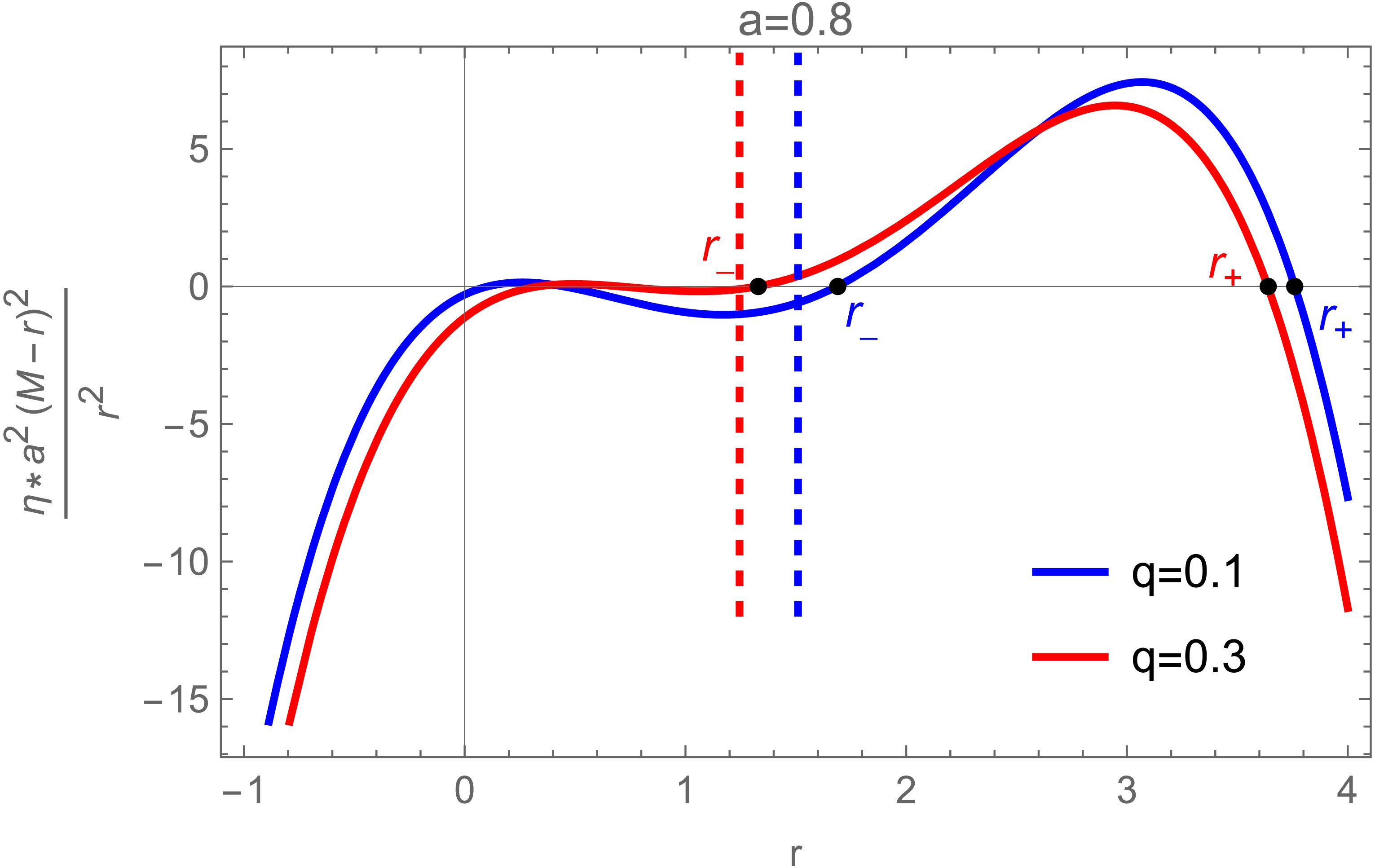
Figure 2. (color online) The dependence of
$ \tilde{\eta} $ on$ \tilde{r} $ is shown. The dashed vertical line indicates the event horizon radius$ r_H $ , while the solid curves show$ \tilde{\eta} $ as a function of$ \tilde{r} $ for different values of the tidal charge q. The curves are plotted for$ a=0.8 $ and$ M=1 $ , with the blue and red curves corresponding to$ q=0.1 $ and$ q=0.3 $ , respectively. -
To investigate photon trajectories around a braneworld black hole, it is essential to examine the dynamical behavior of particles in the corresponding spacetime. Photon trajectories in curved spacetime are governed by the geodesic equation, which reflects the effect of spacetime curvature [37]:
$ \frac{{\rm d}^{2}x^{\mu}}{{\rm d}\lambda^{2}}+ \Gamma^{\mu}_{\alpha\beta}\frac{{\rm d}x^{\alpha}}{{\rm d}\lambda}\frac{{\rm d}x^{\beta}}{{\rm d}\lambda}=0. $
(5) Here, λ is the affine parameter, and
$ \Gamma^{\mu}_{\alpha\beta} $ denotes the Christoffel symbol. Once appropriate initial conditions are specified, the photon path can, in principle, be obtained from this equation, although direct integration is usually impractical.For this reason, we use the Hamilton–Jacobi formalism to describe the geodesic motion. In the present spacetime, the Hamilton–Jacobi equation is given by [38]:
$ \frac{\partial S}{\partial\lambda}+\frac{1}{2}g^{\mu\nu}\frac{\partial S}{\partial x^{\mu}}\frac{\partial S}{\partial x^{\nu}}=0. $
(6) Owing to spacetime symmetries, photon orbits can be described in terms of conserved quantities. For an axisymmetric rotating black hole, three constants of motion are sufficient to determine photon trajectories:
$ p_{t}=-E $ ,$ p_{\phi}=L $ , and$ \mathcal{C}=p_{\theta}^{2}-\cos^{2}\theta\bigl(a^{2}E^{2}-L^{2}\csc^{2}\theta\bigr) $ , where E is the conserved energy, L is the conserved angular momentum, and$ \mathcal{C} $ is the Carter constant. Introducing the dimensionless impact parameters, namely the normalized angular momentum ξ and the rescaled Carter constant η, yields$ \xi=\frac{L}{E},\qquad \eta=\frac{\mathcal{C}}{E^{2}} .$
(7) For braneworld black holes, the photon four-momentum
$ p^{\mu} $ along a trajectory can be written as$ \frac{\Sigma}{E} p^{r} = \pm_{r} \sqrt{{\cal{R}}(r)}, $
(8) $ \frac{\Sigma}{E} p^{\theta} = \pm_{\theta} \sqrt{\Theta(\theta)}, $
(9) $ \frac{\Sigma}{E} p^{\phi} = \frac{\xi}{\sin^{2}{\theta}} + \frac{a(a^{2}+r^{2}-a\xi)}{\Delta} - a, $
(10) $ \frac{\Sigma}{E} p^{t} = a\xi - a^{2}\sin^{2}\theta + \frac{a^{4} + 2a^{2}r^{2} + r^{4} - a\xi(a^{2}+r^{2})}{\Delta}, $
(11) where the radial potential
$ {\cal{R}}(r) $ and the angular potential$ \Theta(\theta) $ are given by$ {\cal{R}}(r) = -\Delta\bigl[(\xi - a)^{2} + \eta\bigr] + (a^{2} + r^{2} - a\xi)^{2}, $
(12) $ \Theta(\theta) = a^{2}\cos^{2}\theta + \eta - \xi^{2}\cot^{2}\theta. $
(13) The symbols
$ \pm_{r} $ and$ \pm_{\theta} $ denote the signs of$ p^{r} $ and$ p^{\theta} $ , respectively. The radial and angular turning points occur at the values of r and θ for which$ {\cal{R}}(r) $ and$ \Theta(\theta) $ vanish. We consider a photon emitted from$ (t_{s}, r_{s}, \theta_{s}, \phi_{s}) $ and received by a distant observer at$ (t_{o}, \infty, \theta_{o}, \phi_{o}) $ . To describe its trajectory, we introduce the Mino time τ.The equations of motion expressed in Mino time take the form [39]
$ \frac{{\rm d}x^{\mu}}{{\rm d}\tau}\equiv\frac{\Sigma}{E}p^{\mu} .$
(14) Using Eqs. (8)–(11), the equations of motion can be recast in the following integral form [39]:
$ \Delta t = t_{o} - t_{s} = I_{t} + a^{2} G_{t}, $
(15) $ \tau = I_{r} = G_{\theta}, $
(16) $ \Delta \phi = \phi_{o} - \phi_{s} = I_{\phi} + \xi G_{\phi}. $
(17) The detailed derivation is provided in Appendix A. The integrals
$ I_{t} $ ,$ I_{r} $ , and$ I_{\phi} $ represent path integrals between the source and observer coordinates,$ x_{s}^{\mu} $ and$ x_{o}^{\mu} $ , respectively. For angular motion with$ \eta \gt 0 $ , the geodesic is described by the polar turning points$ \theta_{\pm} $ , which are symmetric with respect to the equatorial plane [40]:$ \theta_{\pm} = \arccos \left( \mp \sqrt{ \omega_+ } \right), $
(18) where
$ \omega_{\pm} = \frac{1}{2} - \frac{ \eta + \xi^{2} }{ 2 a^{2} } \pm \sqrt{ \frac{ \eta }{ a^{2} } + \frac{1}{4} \left( 1 - \frac{ \eta + \xi^{2} }{ a^{2} } \right)^{2} }. $
(19) To avoid coordinate singularities at the poles, we restrict θ to
$ 0 \lt \theta \lt \pi $ and rewrite the angular potential in terms of$ \omega = \cos^{2}\theta $ . The four roots of$ \Theta(\theta) $ are then$ \theta = \arccos(\pm\sqrt{\omega_{\pm}}) $ .Special cases occur only when
$ \omega_{+}=0 $ ,$ \omega_{-}=0 $ , or$ \omega_{+}=\omega_{-} $ . These conditions divide the$ (\xi,\eta) $ plane into distinct regions. Within each region, the angular potential retains the same qualitative structure, including the number of real roots and the sign of the potential near them. Therefore, the behavior in each region can be effectively characterized by examining a representative point within it.In this formulation, the positive angular integral can be expressed in terms of elliptic integrals and classified according to the number of turning points z along the trajectory. Following Refs. [39, 40], we obtain
$ G_{\theta} = \frac{1}{ a \sqrt{ -\omega_- } } \left[ 2 z K \pm_{s} F_{s} \mp_{o} F_{o} \right], $
(20) $ G_{\phi} = \frac{1}{ a \sqrt{ -\omega_- } } \left[ 2 z \Pi \pm_{s} \Pi_{s} \mp_{o} \Pi_{o} \right], $
(21) $ G_{t} = - \frac{ 2 \omega_+ }{ a \sqrt{ -\omega_- } } \left[ 2 z E' \pm_{s} E'_{s} \mp_{o} E'_{o} \right]. $
(22) Here, K, Π, and
$ E' $ denote the complete elliptic integrals of the first, third, and second kinds, respectively. The quantities$ K_{i} $ ,$ \Pi_{i} $ , and$ E'_{i} $ denote the corresponding incomplete elliptic integrals.In the braneworld black hole spacetime, the tidal charge directly modifies the effective radial potential. By analyzing the roots of this potential, the conserved photon impact parameters, ξ and η, can be obtained explicitly by simultaneously solving Eqs. (2), (3), and (12), yielding:
$ {\cal{R}}(r) = r^{4} + A r^{2} + B r + D, $
(23) where
$ A = a^{2} - \eta - \xi^{2}, $
(24) $ B = 2 M (\eta + \xi^{2} + a^{2} - 2 a \xi), $
(25) $ D = - a^{2} \eta - q (\eta + \xi^{2} + a^{2} - 2 a \xi). $
(26) From Eq. (23), the four roots of the radial potential satisfy
$ r_{1}+r_{2}+r_{3}+r_{4}=0 $ and can be expressed as$ r_{1} = -j - \sqrt{-\frac{A}{2} - j^{2} + \frac{B}{4 j}}, $
(27) $ r_{2} = -j + \sqrt{-\frac{A}{2} - j^{2} + \frac{B}{4 j}}, $
(28) $ r_{3} = j - \sqrt{-\frac{A}{2} - j^{2} - \frac{B}{4 j}}, $
(29) $ r_{4} = j + \sqrt{-\frac{A}{2} - j^{2} - \frac{B}{4 j}}, $
(30) where
$ j = \sqrt{\frac{\varpi_+ + \varpi_- - \dfrac{A}{3}}{2}}, $
(31) $ \varpi_{\pm} = \sqrt[3]{-\frac{A}{6}\left(\frac{A^{2}}{36} - D\right) - \frac{B^{2}}{16} \pm \sqrt{\frac{A^{2}}{36} - \frac{D^{3}}{3} - \frac{A}{6}\left(\frac{A^{2}}{36} - D\right) - \frac{B^{2}}{16}}}. $
(32) For an observer at spatial infinity, a photon trajectory can have at most one radial turning point outside the event horizon. If
$ r_{4} $ is real and lies strictly outside the horizon, the turning point is located at$ r_{4} $ ; otherwise, the photon falls directly into the black hole. Therefore, the radial integral can be written in the generalized form [40]:$ I_t \sim \int_{r_s}^{r_o} {\rm d}r \sim \int_{r_s}^{r_o} \cdots + 2 \omega \int_{r_t}^{r_s} {\rm d}r \cdots. $
(33) In this way, the radial integration takes the following specific form:
$ I_r = \int_{r_s}^{\infty} \frac{{\rm d}r}{\sqrt{{\cal{R}}(r)}} + 2 \omega \int_{r_4}^{r_s} \frac{{\rm d}r}{\sqrt{{\cal{R}}(r)}}. $
(34) where ω is defined in Eqs. (18) and (19). Depending on the light source, two distinct cases should be considered for the total radial integral [40]:
$ I_r^{\rm{total}} = \left\{ \begin{array}{ll} 2\displaystyle\int_{r_s}^{\infty} \frac{{\rm d}r}{\sqrt{{\cal{R}}(r)}}, & r_+ \lt r_4 \in \mathbb{R}, \\ \displaystyle\int_{r_+}^{\infty} \frac{{\rm d}r}{\sqrt{{\cal{R}}(r)}}, & {\rm{otherwise}}. \end{array} \right. $
(35) The root
$ r_{4} $ represents a physical radial turning point only if it is real and lies outside the event horizon. Following the analytical method of Ref. [40], the inverse path integral is obtained by exchanging the observer and source positions. This exchange reverses the direction of integration along the photon path and changes$ I_{r} $ to$ -I_{r} $ . The source radius$ r_{s} $ can then be expressed explicitly as$ r_s = \frac{ r_4 r_{31} - r_3 r_{41}\,{\rm{sn}}^2\left(\dfrac{1}{2}\sqrt{r_{31}r_{42}}\,I_r\right) - {\cal{F}}_o\left|\dfrac{r_{32}r_{41}}{r_{31}r_{42}}\right| }{ r_{31} - r_{41}\,{\rm{sn}}^2\left(\dfrac{1}{2}\sqrt{r_{31}r_{42}}\,I_r\right) - {\cal{F}}_o\left|\dfrac{r_{32}r_{41}}{r_{31}r_{42}}\right| }. $
(36) Here,
$ r_{ij}=r_{i}-r_{j} $ denotes the difference between the corresponding pair of roots, and the auxiliary function$ {\cal{F}}_{o} $ is defined by [40]$ {\cal{F}}_o = F\bigg(\arcsin \sqrt{ \frac{r_{31}}{r_{41}}} | \frac{r_{32}r_{41}}{r_{31}r_{42}} \bigg). $
(37) As in Kerr spacetime, the radial and angular components of photon geodesics in a braneworld black hole can be expressed analytically in terms of elliptic integrals. Because photons may orbit the black hole more than once, we introduce the fractional orbital number
$ n = \frac{G_\theta}{2 \displaystyle\int_{\theta_-}^{\theta_+} {\rm d}\theta \Theta(\theta)^{-{\tfrac{1}{2}}}} = \frac{a \sqrt{-\omega_-}}{4K} I_r. $
(38) Combining Eqs. (20) and (38) yields a derived expression that relates the orbital fraction n to the number of turning points z [39, 40]:
$ n = \frac{1}{2} z \pm_o \frac{1}{4} \left[ (-1)^z \frac{F_s}{K} \mp_o \frac{F_o}{K} \right]. $
(39) For a given pair of impact parameters, ξ and η, the radial potential in Eq. (12) has four roots, given in Eqs. (27)–(30). The real roots correspond to radial turning points. As in the Schwarzschild case, the limiting values of the impact parameters determine the photon-ring location. In the rotating case, the radial potential can develop a double root at a critical radius
$ \tilde{r} $ . The corresponding critical impact parameters,$ \tilde{\xi} $ and$ \tilde{\eta} $ , are determined by$ {\cal{R}}(\tilde{r}) = {\cal{R}}'(\tilde{r}) = 0 $ and can be written as [20]$ \tilde{\xi} = a+\frac{\left[(2a^2+ 2q - 3M\tilde{r} + \tilde{r}^2)\tilde{r}\right]}{a(M - \tilde{r})}, $
(40) $ \tilde{\eta} = -\frac{\tilde{r}^2 \left[4a^2q - 4a^2M\tilde{r} + (2q + \tilde{r}(\tilde{r} - 3M))^2\right]}{a^2(M - \tilde{r})^2}. $
(41) From Eq. (41),
$ \tilde{\eta} $ is a quartic polynomial in$ \tilde{r} $ for a braneworld black hole. Therefore, the standard trigonometric transformations used in simpler cases are not directly applicable. We solve this equation numerically to determine the critical curve accurately. It should also be noted that$ \eta \gt 0 $ for any geodesic crossing the equatorial plane. The photon-shell boundaries are determined by circular photon orbits confined to the equatorial plane, for which$ \tilde{\eta} = 0 $ . Simplifying Eq. (41) gives$ -\tilde{r}^4 + 6M\tilde{r}^3 - (9M^2 + 4q)\tilde{r}^2 + (4a^2M + 12Mq)\tilde{r} - 4(a^2q + q^2) = 0. $
(42) The radial potential
$ {\cal{R}}(r) $ can be expressed as a fourth-degree polynomial,$ {\cal{R}}(r) = (r-\tilde{r}_{1})(r-\tilde{r}_{2})(r-\tilde{r}_{3})(r-\tilde{r}_{4}) $ . The roots are ordered as$ \tilde{r}_{1}<\tilde{r}_{2}<\tilde{r}_{3}<\tilde{r}_{4} $ and satisfy the constraint$ \tilde{r}_{1}+\tilde{r}_{2}+\tilde{r}_{3}+\tilde{r}_{4}=0 $ .Figure 2 shows the dependence of
$ \tilde{\eta} $ on$ \tilde{r} $ , with four roots ordered as$ \tilde{r}_{1}<\tilde{r}_{2}<r_{H}<\tilde{r}_{3}<\tilde{r}_{4} $ . Since the event horizon is located at$ r_{H} $ , only the two roots outside the horizon,$ \tilde{r}_{3} $ and$ \tilde{r}_{4} $ , are physically relevant. We therefore label them$ r_{-} $ and$ r_{+} $ , respectively.
Figure 2. (color online) The dependence of
$ \tilde{\eta} $ on$ \tilde{r} $ is shown. The dashed vertical line indicates the event horizon radius$ r_H $ , while the solid curves show$ \tilde{\eta} $ as a function of$ \tilde{r} $ for different values of the tidal charge q. The curves are plotted for$ a=0.8 $ and$ M=1 $ , with the blue and red curves corresponding to$ q=0.1 $ and$ q=0.3 $ , respectively. -
We consider an observer located at spatial infinity. On the observer’s image plane, the apparent position of a photon is described by the orthogonal celestial coordinates
$ (\alpha, \beta) $ . This configuration maps the observer’s celestial sphere onto a two-dimensional Cartesian plane, where the coordinates scale with trigonometric functions of the photon’s incidence angles. For a braneworld black hole, in which photon trajectories are characterized by two constants of motion, the celestial coordinates α and β are defined as [39, 40]:$ \alpha = -\frac{\xi}{\sin\theta_0}, $
(43) $ \beta = \pm_0 \sqrt{\Theta(\theta)} = \pm_0 \sqrt{\eta + a^2 \cos^2\theta_0 - \xi^2 \cot^2\theta_0} \; . $
(44) In the above expressions, the parameter
$ \theta_{0} $ denotes the observer’s inclination angle. Using the analytical relations derived above, the critical impact parameters$ \xi(\tilde{r}) $ and$ \tilde{\eta}(\tilde{r}) $ can be determined explicitly. Projecting these parameters onto the celestial coordinates$ \tilde{\alpha}(\tilde{r}) $ and$ \tilde{\beta}(\tilde{r}) $ provides a direct characterization of the photon ring on the observer’s screen for a braneworld black hole surrounded by an optically thin accretion disk.Figure 3 presents the photon lensing bands of the braneworld black hole for different observer inclinations, with each image computed at a resolution of
$ 1024 \times 1024 $ pixels. The solid white contour denotes the critical photon curve. We compare three inclination angles,$ \theta_{0}=17^\circ $ ,$ 75^\circ $ , and$ 150^\circ $ . The case$ \theta_{0}=17^\circ $ is close to the inclination inferred for M87$ ^{*} $ from EHT observations. The dark and light gray regions indicate light rays that cross the equatorial plane once and twice, respectively, corresponding to the lensing ring and photon ring. The central dark region is the inner shadow of the braneworld black hole.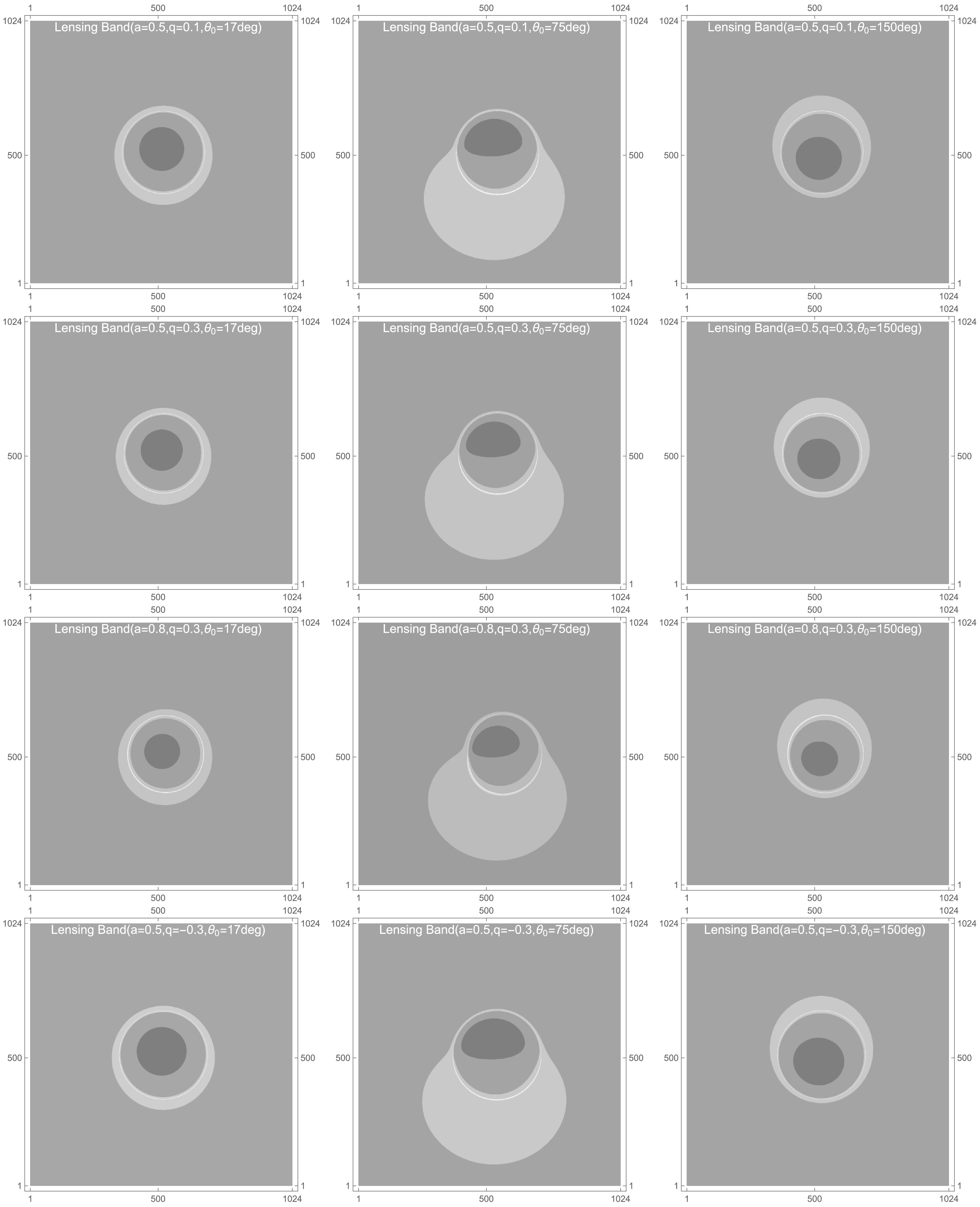
Figure 3. Photon lensing bands around a braneworld black hole are shown for different combinations of the spin parameter a, tidal charge q, and observer inclination angle
$ \theta_{0} $ . The four parameter sets considered are$ a=0.5 $ ,$ q=-0.3 $ ;$ a=0.5 $ ,$ q=0.1 $ ;$ a=0.5 $ ,$ q=0.3 $ ; and$ a=0.8 $ ,$ q=0.3 $ . The corresponding images are presented for inclination angles of$ 17^\circ $ ,$ 75^\circ $ , and$ 150^\circ $ . The dark gray and light gray regions denote light rays that intersect the equatorial plane once and twice, respectively. The white line marks the critical curve, and the innermost region represents the inner shadow of the braneworld black hole. In all cases, the black hole mass is fixed at$ M=1 $ .A comparison of the panels shows that, as the viewing inclination
$ \theta_{0} $ increases from the polar direction toward the equatorial plane, namely within$ 0<\theta_{0}<\pi/2 $ , the critical curve becomes more asymmetric and is gradually stretched toward the southwestern direction on the observer’s screen. This asymmetric deformation mainly arises from frame dragging generated by the black hole rotation, and it becomes stronger as the line of sight moves closer to the equatorial plane. A larger spin further enhances frame dragging and therefore increases the distortion of the critical curve. When the inclination passes the equatorial plane and approaches larger values, the orientation of the critical curve is nearly reversed. This behavior can be interpreted through the intrinsic D-shaped profile of the critical curve for a rotating black hole: changing the viewing direction from$ \theta_{0} $ to$ 180^\circ-\theta_{0} $ approximately produces a mirror-symmetric mapping on the image plane.We now consider photon orbits around the braneworld black hole, focusing mainly on sources in the equatorial plane. For an observer with inclination
$ \theta_{0}\neq 0 $ , the first incomplete elliptic integral$ F_{s} $ vanishes. We then obtain$ \sqrt{-w_-}\, a I_r + {\rm{sign}}(\beta) F_o = 2 z K. $
(45) Here,
$ F_{o} $ denotes the incomplete elliptic integral of the first kind, whereas K denotes the corresponding complete elliptic integral. This equation specifies the functional dependence of the image coordinates$ (\alpha,\beta) $ on the radial source position$ r_{s} $ and the source order z. -
We consider an observer located at spatial infinity. On the observer’s image plane, the apparent position of a photon is described by the orthogonal celestial coordinates
$ (\alpha, \beta) $ . This configuration maps the observer’s celestial sphere onto a two-dimensional Cartesian plane, where the coordinates scale with trigonometric functions of the photon’s incidence angles. For a braneworld black hole, in which photon trajectories are characterized by two constants of motion, the celestial coordinates α and β are defined as [39, 40]:$ \alpha = -\frac{\xi}{\sin\theta_0}, $
(43) $ \beta = \pm_0 \sqrt{\Theta(\theta)} = \pm_0 \sqrt{\eta + a^2 \cos^2\theta_0 - \xi^2 \cot^2\theta_0} \; . $
(44) In the above expressions, the parameter
$ \theta_{0} $ denotes the observer’s inclination angle. Using the analytical relations derived above, the critical impact parameters$ \xi(\tilde{r}) $ and$ \tilde{\eta}(\tilde{r}) $ can be determined explicitly. Projecting these parameters onto the celestial coordinates$ \tilde{\alpha}(\tilde{r}) $ and$ \tilde{\beta}(\tilde{r}) $ provides a direct characterization of the photon ring on the observer’s screen for a braneworld black hole surrounded by an optically thin accretion disk.Figure 3 presents the photon lensing bands of the braneworld black hole for different observer inclinations, with each image computed at a resolution of
$ 1024 \times 1024 $ pixels. The solid white contour denotes the critical photon curve. We compare three inclination angles,$ \theta_{0}=17^\circ $ ,$ 75^\circ $ , and$ 150^\circ $ . The case$ \theta_{0}=17^\circ $ is close to the inclination inferred for M87$ ^{*} $ from EHT observations. The dark and light gray regions indicate light rays that cross the equatorial plane once and twice, respectively, corresponding to the lensing ring and photon ring. The central dark region is the inner shadow of the braneworld black hole.
Figure 3. Photon lensing bands around a braneworld black hole are shown for different combinations of the spin parameter a, tidal charge q, and observer inclination angle
$ \theta_{0} $ . The four parameter sets considered are$ a=0.5 $ ,$ q=-0.3 $ ;$ a=0.5 $ ,$ q=0.1 $ ;$ a=0.5 $ ,$ q=0.3 $ ; and$ a=0.8 $ ,$ q=0.3 $ . The corresponding images are presented for inclination angles of$ 17^\circ $ ,$ 75^\circ $ , and$ 150^\circ $ . The dark gray and light gray regions denote light rays that intersect the equatorial plane once and twice, respectively. The white line marks the critical curve, and the innermost region represents the inner shadow of the braneworld black hole. In all cases, the black hole mass is fixed at$ M=1 $ .A comparison of the panels shows that, as the viewing inclination
$ \theta_{0} $ increases from the polar direction toward the equatorial plane, namely within$ 0<\theta_{0}<\pi/2 $ , the critical curve becomes more asymmetric and is gradually stretched toward the southwestern direction on the observer’s screen. This asymmetric deformation mainly arises from frame dragging generated by the black hole rotation, and it becomes stronger as the line of sight moves closer to the equatorial plane. A larger spin further enhances frame dragging and therefore increases the distortion of the critical curve. When the inclination passes the equatorial plane and approaches larger values, the orientation of the critical curve is nearly reversed. This behavior can be interpreted through the intrinsic D-shaped profile of the critical curve for a rotating black hole: changing the viewing direction from$ \theta_{0} $ to$ 180^\circ-\theta_{0} $ approximately produces a mirror-symmetric mapping on the image plane.We now consider photon orbits around the braneworld black hole, focusing mainly on sources in the equatorial plane. For an observer with inclination
$ \theta_{0}\neq 0 $ , the first incomplete elliptic integral$ F_{s} $ vanishes. We then obtain$ \sqrt{-w_-}\, a I_r + {\rm{sign}}(\beta) F_o = 2 z K. $
(45) Here,
$ F_{o} $ denotes the incomplete elliptic integral of the first kind, whereas K denotes the corresponding complete elliptic integral. This equation specifies the functional dependence of the image coordinates$ (\alpha,\beta) $ on the radial source position$ r_{s} $ and the source order z. -
We now examine the observational appearance of a braneworld black hole illuminated by an optically thin accretion disk. Following the standard relativistic disk model, we assume that the accreting material moves along quasi-circular geodesics in the equatorial plane. The inner edge of the disk is assumed to lie at the innermost stable circular orbit (ISCO). Physically, the ISCO marks the transition between stable and unstable circular orbits. Under radial perturbations, particles crossing this threshold lose orbital stability, move rapidly inward, and eventually plunge into the black hole.
As test particles move inward toward the ISCO of a braneworld black hole, their orbital velocities increase. To account for these relativistic kinematic effects, we extend the emitting region of the accretion disk inward toward the event horizon. In this disk model, the innermost emitting edge is placed close to the event horizon, while the main body of the disk extends outside the ISCO. This treatment requires two additional considerations:
1. Gravitational redshift and radiative-transfer effects near the ISCO must be carefully re-evaluated.
2. Ray tracing must be performed over an extended radial interval.
For a massive particle confined to the equatorial plane, we define the conserved specific energy and angular momentum as
$ {\cal{E}}=-u_t $ and$ {\cal{L}}=u_\phi $ , respectively. As derived in Appendix B, the inward-directed radial component of the four-velocity can be written as$ u^r = -\sqrt{ -\frac{ V(r,{\cal{E}},{\cal{L}}) }{ g_{rr} } }. $
(46) Here, the negative sign corresponds to the inward-moving branch, and the effective potential is defined by
$ V(r,{\cal{E}},{\cal{L}}) = \left[ 1 +g^{tt}{\cal{E}}^{2} -2g^{t\phi}{\cal{E}}{\cal{L}} +g^{\phi\phi}{\cal{L}}^{2} \right]_{\theta=\pi/2}. $
(47) Using Eq. (47), we describe the radial motion of test particles in terms of the effective potential. Figure 4 shows the radial profiles of
$ -V_{\rm{eff}} $ for different spin parameters a and tidal charges q. For fixed spin, increasing q decreases the maximum of$ -V_{\rm{eff}} $ and shifts its location to a larger radius. Similar behavior is observed when the spin is increased at fixed tidal charge. The differences among the curves are most pronounced near the black hole, whereas they gradually diminish at larger radii.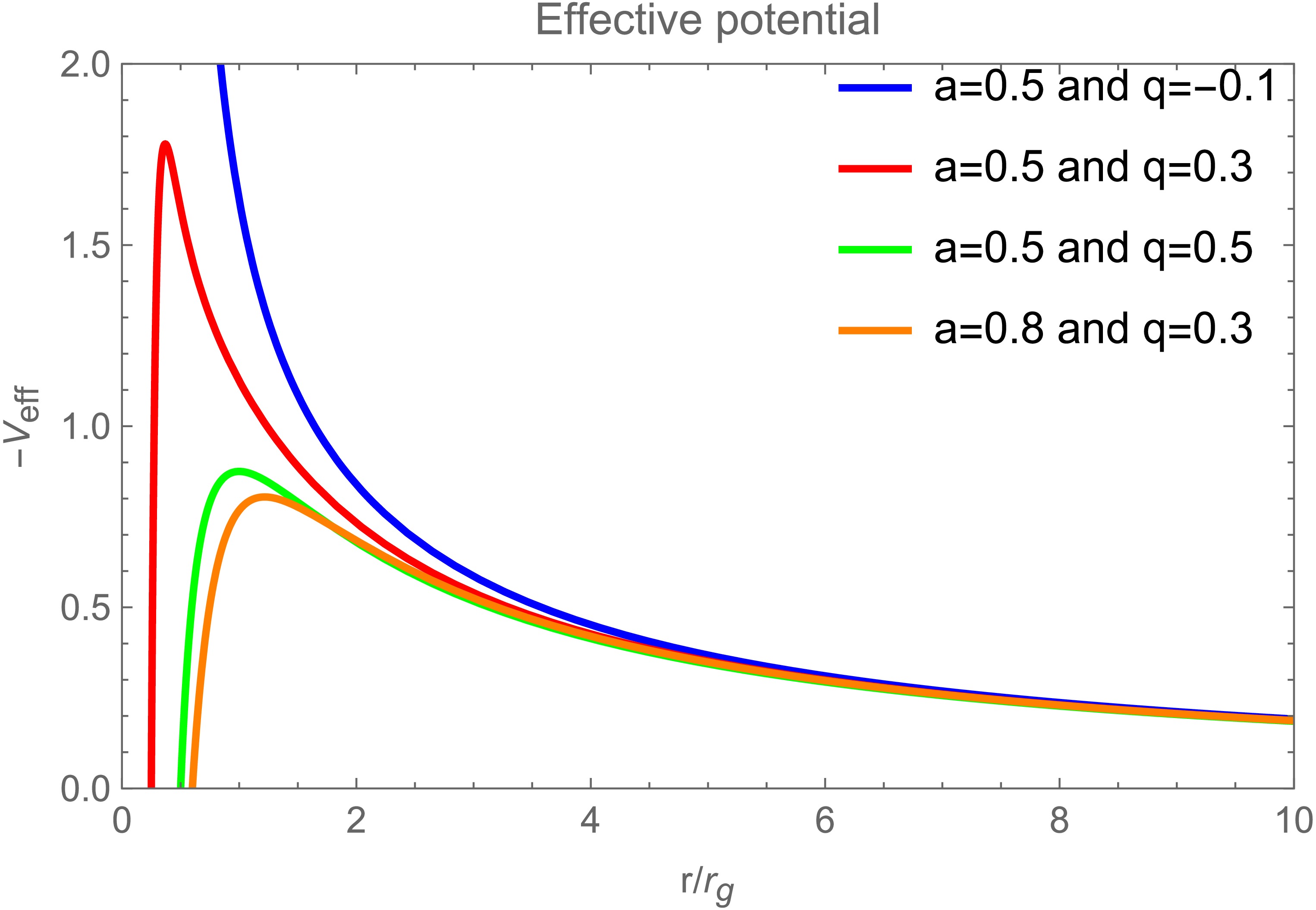
Figure 4. (color online) Profiles of the effective potential as functions of radius for test particles around the braneworld black hole. Four parameter sets are shown:
$ a=0.5 $ ,$ q=-0.1 $ ;$ a=0.5 $ ,$ q=0.3 $ ;$ a=0.5 $ ,$ q=0.5 $ ; and$ a=0.8 $ ,$ q=0.3 $ , illustrating the effects of black hole spin and tidal charge. The peak of the effective potential shifts outward and decreases in amplitude as either parameter increases. The plot uses the convention$ M=1 $ for the black hole mass.For a circular equatorial orbit, the radial velocity vanishes. The ISCO is determined by the simultaneous marginal-stability conditions
$ V=0 $ ,$ \partial_rV=0 $ , and$ \partial_r^2V=0 $ , where the radial derivatives are evaluated with$ {\cal{E}} $ and$ {\cal{L}} $ held fixed. The corresponding physical root outside the event horizon is denoted by$ r_{\rm{ISCO}} $ .Inside the ISCO, stable circular motion is no longer possible. Following the Cunningham-type prescription adopted in this work, the conserved quantities of the plunging matter are set to their ISCO values,
$ {\cal{E}}={\cal{E}}_{\rm{ISCO}} $ and$ {\cal{L}}={\cal{L}}_{\rm{ISCO}} $ . Equation (46) then becomes$ u^r=-\sqrt{-\frac{V\left(r,{\cal{E}}_{\rm{ISCO}}, {\cal{L}}_{\rm{ISCO}} \right)}{g_{rr}}},\qquad r_H\leqslant r<r_{\rm{ISCO}}. $
(48) The explicit expressions for
$ r_{\rm{ISCO}} $ ,$ {\cal{E}}_{\rm{ISCO}} $ ,$ {\cal{L}}_{\rm{ISCO}} $ , and the full plunging four-velocity$ u^\mu=(u^t,u^r,0,u^\phi) $ are presented in Appendix C. The upper and lower signs therein correspond consistently to the prograde and retrograde branches, respectively. -
We now examine the observational appearance of a braneworld black hole illuminated by an optically thin accretion disk. Following the standard relativistic disk model, we assume that the accreting material moves along quasi-circular geodesics in the equatorial plane. The inner edge of the disk is assumed to lie at the innermost stable circular orbit (ISCO). Physically, the ISCO marks the transition between stable and unstable circular orbits. Under radial perturbations, particles crossing this threshold lose orbital stability, move rapidly inward, and eventually plunge into the black hole.
As test particles move inward toward the ISCO of a braneworld black hole, their orbital velocities increase. To account for these relativistic kinematic effects, we extend the emitting region of the accretion disk inward toward the event horizon. In this disk model, the innermost emitting edge is placed close to the event horizon, while the main body of the disk extends outside the ISCO. This treatment requires two additional considerations:
1. Gravitational redshift and radiative-transfer effects near the ISCO must be carefully re-evaluated.
2. Ray tracing must be performed over an extended radial interval.
For a massive particle confined to the equatorial plane, we define the conserved specific energy and angular momentum as
$ {\cal{E}}=-u_t $ and$ {\cal{L}}=u_\phi $ , respectively. As derived in Appendix B, the inward-directed radial component of the four-velocity can be written as$ u^r = -\sqrt{ -\frac{ V(r,{\cal{E}},{\cal{L}}) }{ g_{rr} } }. $
(46) Here, the negative sign corresponds to the inward-moving branch, and the effective potential is defined by
$ V(r,{\cal{E}},{\cal{L}}) = \left[ 1 +g^{tt}{\cal{E}}^{2} -2g^{t\phi}{\cal{E}}{\cal{L}} +g^{\phi\phi}{\cal{L}}^{2} \right]_{\theta=\pi/2}. $
(47) Using Eq. (47), we describe the radial motion of test particles in terms of the effective potential. Figure 4 shows the radial profiles of
$ -V_{\rm{eff}} $ for different spin parameters a and tidal charges q. For fixed spin, increasing q decreases the maximum of$ -V_{\rm{eff}} $ and shifts its location to a larger radius. Similar behavior is observed when the spin is increased at fixed tidal charge. The differences among the curves are most pronounced near the black hole, whereas they gradually diminish at larger radii.
Figure 4. (color online) Profiles of the effective potential as functions of radius for test particles around the braneworld black hole. Four parameter sets are shown:
$ a=0.5 $ ,$ q=-0.1 $ ;$ a=0.5 $ ,$ q=0.3 $ ;$ a=0.5 $ ,$ q=0.5 $ ; and$ a=0.8 $ ,$ q=0.3 $ , illustrating the effects of black hole spin and tidal charge. The peak of the effective potential shifts outward and decreases in amplitude as either parameter increases. The plot uses the convention$ M=1 $ for the black hole mass.For a circular equatorial orbit, the radial velocity vanishes. The ISCO is determined by the simultaneous marginal-stability conditions
$ V=0 $ ,$ \partial_rV=0 $ , and$ \partial_r^2V=0 $ , where the radial derivatives are evaluated with$ {\cal{E}} $ and$ {\cal{L}} $ held fixed. The corresponding physical root outside the event horizon is denoted by$ r_{\rm{ISCO}} $ .Inside the ISCO, stable circular motion is no longer possible. Following the Cunningham-type prescription adopted in this work, the conserved quantities of the plunging matter are set to their ISCO values,
$ {\cal{E}}={\cal{E}}_{\rm{ISCO}} $ and$ {\cal{L}}={\cal{L}}_{\rm{ISCO}} $ . Equation (46) then becomes$ u^r=-\sqrt{-\frac{V\left(r,{\cal{E}}_{\rm{ISCO}}, {\cal{L}}_{\rm{ISCO}} \right)}{g_{rr}}},\qquad r_H\leqslant r<r_{\rm{ISCO}}. $
(48) The explicit expressions for
$ r_{\rm{ISCO}} $ ,$ {\cal{E}}_{\rm{ISCO}} $ ,$ {\cal{L}}_{\rm{ISCO}} $ , and the full plunging four-velocity$ u^\mu=(u^t,u^r,0,u^\phi) $ are presented in Appendix C. The upper and lower signs therein correspond consistently to the prograde and retrograde branches, respectively. -
To rigorously model a fisheye camera and define the observer’s local reference frame, we introduce a standard orthonormal tetrad that provides a local basis at each point in spacetime [41]. In the braneworld black hole spacetime, the observer’s orthonormal tetrad can be expressed as [41, 42]
$ e_t = \delta \, \partial_t + \chi \, \partial_\phi, \quad e_r = \frac{1}{\sqrt{g_{rr}}} \, \partial_r, $
(49) $ e_\theta = \frac{1}{\sqrt{g_{\theta\theta}}} \, \partial_\theta, \quad e_\phi = \frac{1}{\sqrt{g_{\phi\phi}}\partial_\phi} , $
(50) where
$ \delta = \sqrt{\frac{g_{\phi\phi}}{g_{t\phi}^2 - g_{tt} g_{\phi\phi}}}, \quad \chi = -\frac{g_{t\phi}}{g_{\phi\phi}} \sqrt{\frac{g_{\phi\phi}}{g_{t\phi}^2 - g_{tt} g_{\phi\phi}}}. $
(51) In the ZAMO frame, photon trajectories are reversible; therefore, photons arriving at the observer can be traced backward to their emission points. The photon four-momentum measured in the local tetrad frame can then be transformed to the coordinate basis. Thus, the four-momentum
$ p^{\mu} $ is given by$ p^\mu = \eta^{\mu\nu} e^\xi_\nu k_\xi . $
(52) The explicit components of the four-momentum are defined as follows [16, 40]:
$ P^t = E \left( \delta - \chi \xi \right), \quad P^r = E \, \frac{1}{\sqrt{g_{rr}}} \, \frac{\pm_r \sqrt{R(r)}}{\Delta_r}, $
(53) $ P^\theta = E \, \frac{1}{\sqrt{g_{\theta\theta}}} \, \frac{\pm_\theta \sqrt{\Theta(\theta)}}{\Delta_\theta}, \quad P^\phi = E \, \frac{\xi}{\sqrt{g_{\phi\phi}}}. $
(54) To show more clearly how the inner shadow of the braneworld black hole changes, the corresponding regions in Fig. 5 are enlarged in Fig. 6. The inner shadow becomes progressively more distorted as the tidal charge and spin increase. Its morphology is particularly more sensitive to the spin parameter than to the tidal charge.
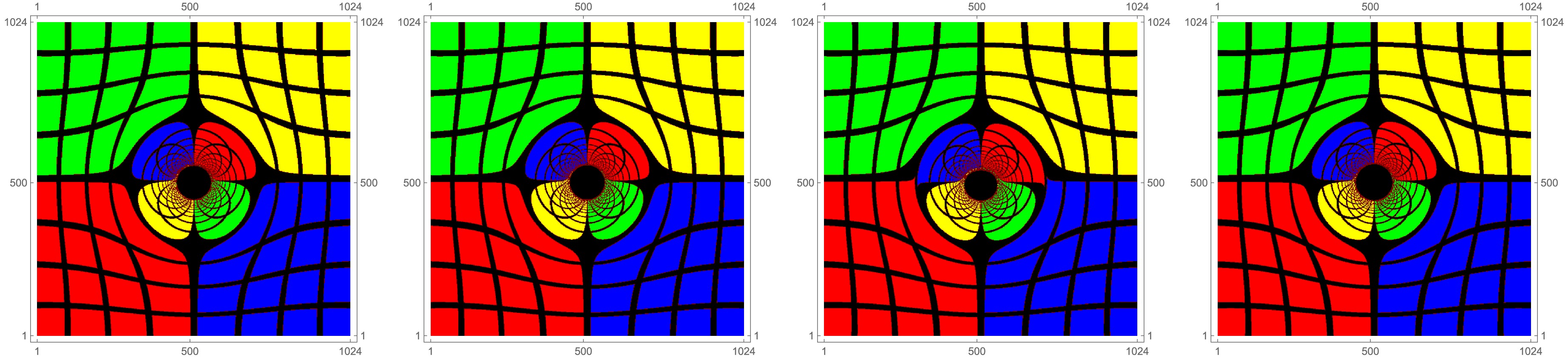
Figure 5. (color online) The shadow cast by the braneworld black hole is investigated using numerical ray tracing. From left to right, the parameter sets are
$ a=0.5 $ ,$ q=-0.3 $ ;$ a=0.5 $ ,$ q=0 $ (Kerr);$ a=0.5 $ ,$ q=0.3 $ ; and$ a=0.8 $ ,$ q=0.3 $ . All images use the convention$ M=1 $ for the black hole mass, and the observer inclination angle is fixed at$ 17^\circ $ .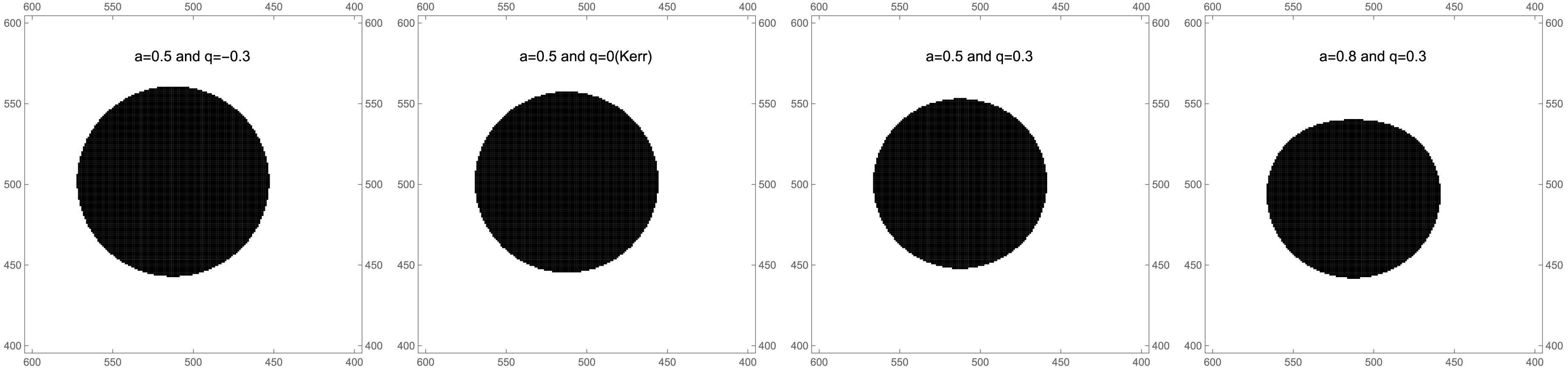
Figure 6. The inner shadow of the braneworld black hole is examined using four parameter sets, shown from left to right:
$ a=0.5 $ ,$ q=-0.3 $ ;$ a=0.5 $ ,$ q=0 $ (Kerr);$ a=0.5 $ ,$ q=0.3 $ ; and$ a=0.8 $ ,$ q=0.3 $ . All images adopt the convention$ M=1 $ for the black hole mass, and the observer inclination angle is fixed at$ 17^\circ $ .Figure 7 shows the inner shadow of the braneworld black hole for different values of the observer inclination, tidal charge, and spin parameter. For a controlled comparison, four inner-shadow images are superposed in each panel, revealing the following trends:
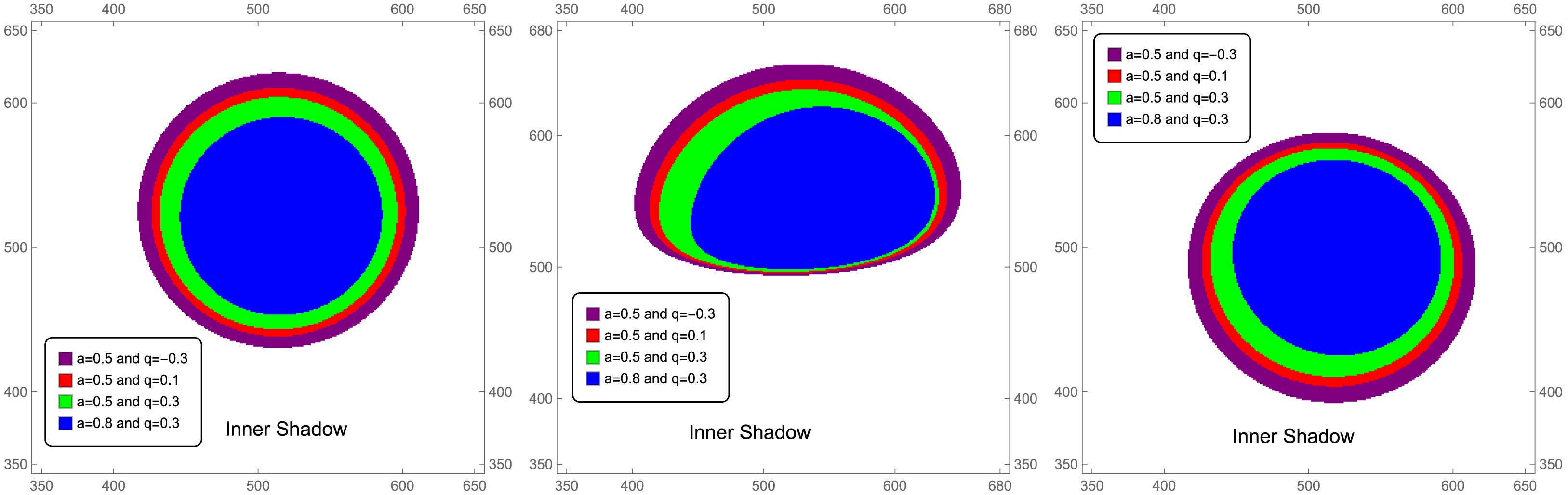
Figure 7. (color online) A comparison of the black hole inner shadow is presented for four parameter sets:
$ a=0.5,\,q=-0.3 $ ,$ a=0.5, $ $ q=0.1 $ ,$ a=0.5,\,q=0.3 $ , and$ a=0.8,\,q=0.3 $ . These cases are analyzed for three observer inclination angles. From left to right, the columns correspond to$ \theta_{0}=17^\circ $ ,$ 75^\circ $ , and$ 150^\circ $ . In all panels, the black hole mass is set to$ M=1 $ .● As the observer inclination increases from
$ 0^\circ $ to$ 90^\circ $ , the inner shadow becomes progressively flattened. At inclination angles greater than$ 90^\circ $ , this deformation gradually decreases.● As the tidal charge increases, the effective gravitational field is altered, causing the inner shadow to shrink.
● Similarly, an increase in the spin parameter strengthens the frame-dragging effect induced by the black hole’s rotation, thereby reducing the size of the inner shadow.
● For all observer inclination angles, the deformation of the inner shadow is more sensitive to variations in the spin parameter than to changes in the tidal charge.
Table 1 compares the effective shadow eccentricity of Kerr and rotating braneworld black holes at
$ \theta_0=17^\circ $ . The Kerr limit is recovered for$ q=0 $ . For a fixed spin, a negative tidal charge decreases the effective shadow eccentricity, whereas a positive tidal charge increases it. This behavior indicates that the tidal charge can modify the global deformation of the black hole shadow. Moreover, the variation in$ \Delta e_{\rm{sh}} $ becomes more pronounced for the higher-spin case, indicating that the deformation effect is enhanced when the black hole rotates faster.Model a q $ e_{\rm{sh}} $ $ \Delta e_{\rm{sh}} $ Kerr 0.5 0 0.0533767 0 Braneworld 0.5 $ -0.3 $ 0.0457269 $ -0.0076498 $ Braneworld 0.5 $ -0.1 $ 0.0504692 $ -0.0029075 $ Braneworld 0.5 0.1 0.0567748 0.0033981 Braneworld 0.5 0.3 0.0657453 0.0123686 Kerr 0.8 0 0.102891 0 Braneworld 0.8 $ -0.3 $ 0.0836967 $ -0.0191943 $ Braneworld 0.8 $ -0.1 $ 0.0952338 $ -0.0076572 $ Braneworld 0.8 0.1 0.112556 0.009665 Braneworld 0.8 0.3 0.143703 0.040812 Table 1. Comparison of the effective shadow eccentricity for Kerr and rotating braneworld black holes at an observer inclination angle of
$ \theta_0=17^\circ $ . The Kerr case is recovered by setting$ q=0 $ . The quantity$ \Delta e_{\rm{sh}}=e_{\rm{sh}}(a,q)-e_{\rm{sh}}(a,0) $ measures the additional global deformation induced by the braneworld tidal charge at fixed spin. -
To rigorously model a fisheye camera and define the observer’s local reference frame, we introduce a standard orthonormal tetrad that provides a local basis at each point in spacetime [41]. In the braneworld black hole spacetime, the observer’s orthonormal tetrad can be expressed as [41, 42]
$ e_t = \delta \, \partial_t + \chi \, \partial_\phi, \quad e_r = \frac{1}{\sqrt{g_{rr}}} \, \partial_r, $
(49) $ e_\theta = \frac{1}{\sqrt{g_{\theta\theta}}} \, \partial_\theta, \quad e_\phi = \frac{1}{\sqrt{g_{\phi\phi}}\partial_\phi} , $
(50) where
$ \delta = \sqrt{\frac{g_{\phi\phi}}{g_{t\phi}^2 - g_{tt} g_{\phi\phi}}}, \quad \chi = -\frac{g_{t\phi}}{g_{\phi\phi}} \sqrt{\frac{g_{\phi\phi}}{g_{t\phi}^2 - g_{tt} g_{\phi\phi}}}. $
(51) In the ZAMO frame, photon trajectories are reversible; therefore, photons arriving at the observer can be traced backward to their emission points. The photon four-momentum measured in the local tetrad frame can then be transformed to the coordinate basis. Thus, the four-momentum
$ p^{\mu} $ is given by$ p^\mu = \eta^{\mu\nu} e^\xi_\nu k_\xi . $
(52) The explicit components of the four-momentum are defined as follows [16, 40]:
$ P^t = E \left( \delta - \chi \xi \right), \quad P^r = E \, \frac{1}{\sqrt{g_{rr}}} \, \frac{\pm_r \sqrt{R(r)}}{\Delta_r}, $
(53) $ P^\theta = E \, \frac{1}{\sqrt{g_{\theta\theta}}} \, \frac{\pm_\theta \sqrt{\Theta(\theta)}}{\Delta_\theta}, \quad P^\phi = E \, \frac{\xi}{\sqrt{g_{\phi\phi}}}. $
(54) To show more clearly how the inner shadow of the braneworld black hole changes, the corresponding regions in Fig. 5 are enlarged in Fig. 6. The inner shadow becomes progressively more distorted as the tidal charge and spin increase. Its morphology is particularly more sensitive to the spin parameter than to the tidal charge.
Figure 5. (color online) The shadow cast by the braneworld black hole is investigated using numerical ray tracing. From left to right, the parameter sets are
$ a=0.5 $ ,$ q=-0.3 $ ;$ a=0.5 $ ,$ q=0 $ (Kerr);$ a=0.5 $ ,$ q=0.3 $ ; and$ a=0.8 $ ,$ q=0.3 $ . All images use the convention$ M=1 $ for the black hole mass, and the observer inclination angle is fixed at$ 17^\circ $ .
Figure 6. The inner shadow of the braneworld black hole is examined using four parameter sets, shown from left to right:
$ a=0.5 $ ,$ q=-0.3 $ ;$ a=0.5 $ ,$ q=0 $ (Kerr);$ a=0.5 $ ,$ q=0.3 $ ; and$ a=0.8 $ ,$ q=0.3 $ . All images adopt the convention$ M=1 $ for the black hole mass, and the observer inclination angle is fixed at$ 17^\circ $ .Figure 7 shows the inner shadow of the braneworld black hole for different values of the observer inclination, tidal charge, and spin parameter. For a controlled comparison, four inner-shadow images are superposed in each panel, revealing the following trends:
Figure 7. (color online) A comparison of the black hole inner shadow is presented for four parameter sets:
$ a=0.5,\,q=-0.3 $ ,$ a=0.5, $ $ q=0.1 $ ,$ a=0.5,\,q=0.3 $ , and$ a=0.8,\,q=0.3 $ . These cases are analyzed for three observer inclination angles. From left to right, the columns correspond to$ \theta_{0}=17^\circ $ ,$ 75^\circ $ , and$ 150^\circ $ . In all panels, the black hole mass is set to$ M=1 $ .● As the observer inclination increases from
$ 0^\circ $ to$ 90^\circ $ , the inner shadow becomes progressively flattened. At inclination angles greater than$ 90^\circ $ , this deformation gradually decreases.● As the tidal charge increases, the effective gravitational field is altered, causing the inner shadow to shrink.
● Similarly, an increase in the spin parameter strengthens the frame-dragging effect induced by the black hole’s rotation, thereby reducing the size of the inner shadow.
● For all observer inclination angles, the deformation of the inner shadow is more sensitive to variations in the spin parameter than to changes in the tidal charge.
Table 1 compares the effective shadow eccentricity of Kerr and rotating braneworld black holes at
$ \theta_0=17^\circ $ . The Kerr limit is recovered for$ q=0 $ . For a fixed spin, a negative tidal charge decreases the effective shadow eccentricity, whereas a positive tidal charge increases it. This behavior indicates that the tidal charge can modify the global deformation of the black hole shadow. Moreover, the variation in$ \Delta e_{\rm{sh}} $ becomes more pronounced for the higher-spin case, indicating that the deformation effect is enhanced when the black hole rotates faster.Model a q $ e_{\rm{sh}} $ $ \Delta e_{\rm{sh}} $ Kerr 0.5 0 0.0533767 0 Braneworld 0.5 $ -0.3 $ 0.0457269 $ -0.0076498 $ Braneworld 0.5 $ -0.1 $ 0.0504692 $ -0.0029075 $ Braneworld 0.5 0.1 0.0567748 0.0033981 Braneworld 0.5 0.3 0.0657453 0.0123686 Kerr 0.8 0 0.102891 0 Braneworld 0.8 $ -0.3 $ 0.0836967 $ -0.0191943 $ Braneworld 0.8 $ -0.1 $ 0.0952338 $ -0.0076572 $ Braneworld 0.8 0.1 0.112556 0.009665 Braneworld 0.8 0.3 0.143703 0.040812 Table 1. Comparison of the effective shadow eccentricity for Kerr and rotating braneworld black holes at an observer inclination angle of
$ \theta_0=17^\circ $ . The Kerr case is recovered by setting$ q=0 $ . The quantity$ \Delta e_{\rm{sh}}=e_{\rm{sh}}(a,q)-e_{\rm{sh}}(a,0) $ measures the additional global deformation induced by the braneworld tidal charge at fixed spin. -
When analyzing photons emitted from the accretion disk that reach the observer’s image plane, it is essential to account for variations in the observed intensity due to scattering, absorption, Doppler boosting, and gravitational redshift. With these effects included, the radiative transfer equation governs the intensity measured by the observer [43]:
$ \frac{{\rm d}}{{\rm d}\lambda}\left(\frac{I_\nu}{\nu^3}\right) = \frac{J_\nu - \kappa_\nu I_\nu}{\nu^2}, $
(55) Here, λ is the affine parameter, while
$ I_{\nu} $ ,$ J_{\nu} $ , and$ \kappa_{\nu} $ denote the specific intensity, emission coefficient, and absorption coefficient at frequency ν, respectively. In vacuum,$ J_{\nu} $ and$ \kappa_{\nu} $ vanish; thus,$ I_{\nu}/\nu^{3} $ is conserved along the geodesic. Under the assumption that the accretion disk is geometrically and optically thin, the intensity profile on the observer’s image plane is obtained by integrating the photon trajectories. The observed intensity is therefore [12]$ I_{\nu_0} = \sum\limits_{m=1}^{N_{\rm{max}}} \left(\frac{\nu_0}{\nu_m}\right)^3 J_m \, \frac{1 - {\rm e}^{-\kappa_m \tau_{m-1}}}{\kappa_m}\, . $
(56) Here,
$ \nu_{0} $ denotes the photon frequency on the observer’s image plane,$ \nu_{m} $ denotes the frequency measured in the disk comoving frame, and$ \tau_{k} $ is the optical depth for photons emitted at point k. Accounting for the physical properties of the accretion disk, Eq. (56) can be simplified to$ I_{\nu_0} = \sum\limits_{m=1}^{N_{\max}} f_m \, g^3(r_m) \, J_{\rm model}(r_m), $
(57) where
$ f_{m} $ denotes a weighting factor,$ g(r_{m}) $ is the frequency-shift factor, and$J_{\rm model}(r_{m})$ represents the emissivity model evaluated at the emission radius$ r_{m} $ .In the following, we consider radiation emitted from the equatorial plane. For each image-plane coordinate
$ (\alpha,\beta) $ ,$ N_{\max}(\alpha,\beta) $ gives the number of intersections between the photon geodesic and the equatorial plane. For$ N_{\max}=1 $ , the geodesic crosses the equatorial plane only once, producing a direct image of the equatorial emission. For$ N_{\max}=2,3,4,\ldots $ multiple intersections occur, producing lensed and higher-order images.The radius
$ r_{m}(\alpha,\beta) $ is the radial position at which the geodesic associated with$ (\alpha,\beta) $ crosses the equatorial plane. Thus, the image order is determined by the number of equatorial-plane intersections rather than by the number of radial or angular turning points.In Eq. (57),
$J_{\rm model}(r_{m})$ is the emissivity evaluated at the emission radius$ r_{m} $ on the equatorial plane, g is the combined gravitational and Doppler frequency-shift factor, and$ f_{m} $ is a correction factor that adjusts the luminosity contribution from higher-order photon-ring images [39]. For the geometrically thin and optically thin disk considered here, we set$ f_{m}=1.5 $ throughout the analysis. The emissivity profile$J_{\rm model}(r)$ is modeled as [15]$ \log[J_{\rm model}(r)] = A \, \log \left(\frac{r}{r_H}\right) + B \left[\log \left(\frac{r}{r_H}\right)\right]^2, $
(58) where A and B are model-dependent fitting parameters, and
$ r_{H} $ denotes the black hole event horizon radius.At 230 GHz, the corresponding observing wavelength for M87
$ ^{*} $ and Sgr A$ ^{*} $ is 1.3 mm. We adopt$ A=-2 $ and$ B=-{1}/{2} $ at this frequency. At 86 GHz, we set$ A=0 $ and$ B=-{3}/{4} $ [15]. Using these values, we calculate the luminosity of the braneworld black hole within the thin-disk model. Figure 8 presents a comparison of the frequency at 230 GHz and 86 GHz.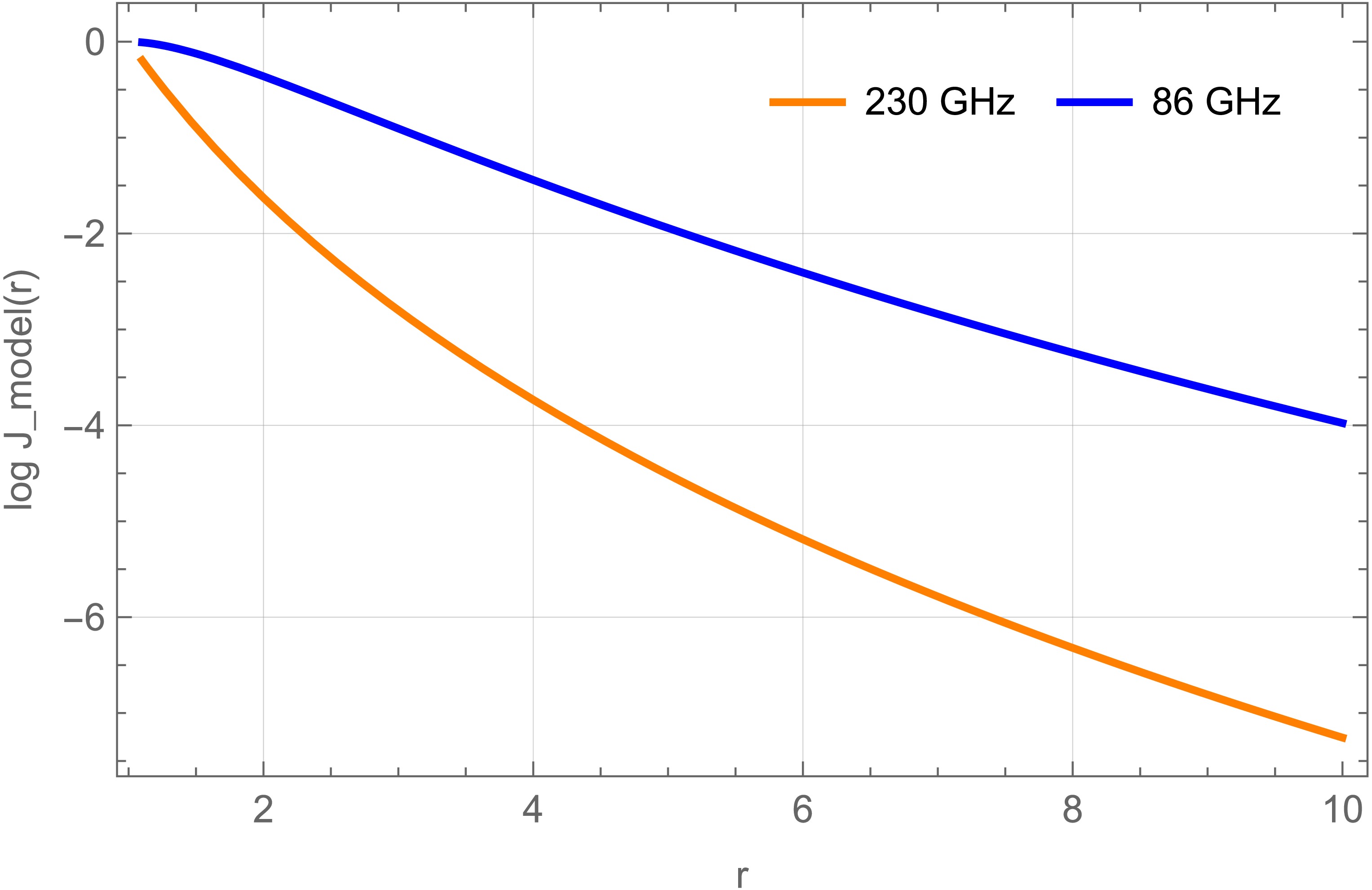
Figure 8. (color online) Comparison of the accretion-disk emissivity profiles at 230 GHz and 86 GHz, with the event horizon radius fixed at
$ r_{H}=1 $ . In all cases, the black hole mass is set to$ M=1 $ .The frequency-shift factor is defined as
$ g=\nu_{0}/\nu_{m} $ . The disk model used here extends previous models by allowing radiation from the disk’s inner edge to reach the event horizon, thereby enabling a more detailed analysis of frequency-shift effects. Outside the ISCO, the accretion flow remains on circular orbits with angular velocity$ \Omega_{m}(r)=\left.\dfrac{u^{\phi}}{u^{t}}\right|_{r=r_{m}} $ .The parameter ξ is defined in Eq. (7), whereas ϵ measures the ratio of the observed energy to the conserved energy along the geodesic [12]:
$ \epsilon = \frac{E_0}{{\cal{E}}} = \frac{P_t}{k_t} = \delta \,(1 + \xi \chi). $
(59) The quantities χ and δ are defined in Eq. (51). Because the spacetime is asymptotically flat,
$ \epsilon=1 $ . For an emission radius$ r_{m} $ outside the ISCO, the frequency-shift factor therefore becomes [12]$ g_m = \frac{\epsilon}{\zeta \,(1 - \xi \Omega_m)}, \quad r_m \gt r_{\rm ISCO}, $
(60) where
$ \zeta = \sqrt{-\frac{1}{g_{tt} + 2 g_{t\phi} \Omega_m + g_{\phi\phi} \Omega_m^2}} \,\bigg|_{r = r_m}. $
(61) As discussed above, the ISCO determines the radial location of the inner boundary of the accretion disk. Inside the ISCO, the flow enters the plunging region and develops a radial velocity
$ u^{r}_{c} $ . In this region, the frequency-shift factor is$ g_m = \frac{\epsilon}{- \dfrac{u^r_c k_r}{k_t} + g^{tt} {\cal{E}}_{\rm{ISCO}} - \xi g^{t\phi} {\cal{E}}_{\rm{ISCO}} - g^{t\phi} {\cal{L}}_{\rm{ISCO}}+ \xi g^{\phi\phi} {\cal{L}}_{\rm{ISCO}}}. $
(62) For a clearer presentation of the frequency-shift distribution, the radial coordinate of the observer is set to
$ r_{o}=100R_{s} $ , where$ R_{s} $ is the Schwarzschild radius, and the image-plane angle is chosen as$ \phi=\pi/10 $ . Both prograde and retrograde disk rotations are included. Photons are classified according to whether they are emitted in the same direction as, or opposite to, the black hole rotation. This distinction is important because the direction of disk rotation strongly affects both the observed frequency shift and the photon trajectories near the braneworld black hole.Here, ''first-order'' and ''second-order'' refer to the number of intersections between a photon trajectory and the equatorial emitting plane, rather than to a perturbative expansion of the frequency-shift factor. The first-order map mainly represents the direct image, while the second-order map corresponds to the lensed image. Their comparison illustrates how stronger gravitational lensing modifies the observed frequency-shift distribution.
Figures 9–12 display the first- and second-order frequency-shift maps and show the kinematic imprint of the optically thin disk in both prograde and retrograde configurations. As the observer inclination
$ \theta_0 $ changes from$ 0^\circ $ toward$ 90^\circ $ , the redshifted area becomes smaller, while the blueshifted region expands. When$ \theta_0 $ increases further from$ 90^\circ $ to$ 180^\circ $ , the trend is reversed: the redshifted region grows again and the blueshifted area contracts.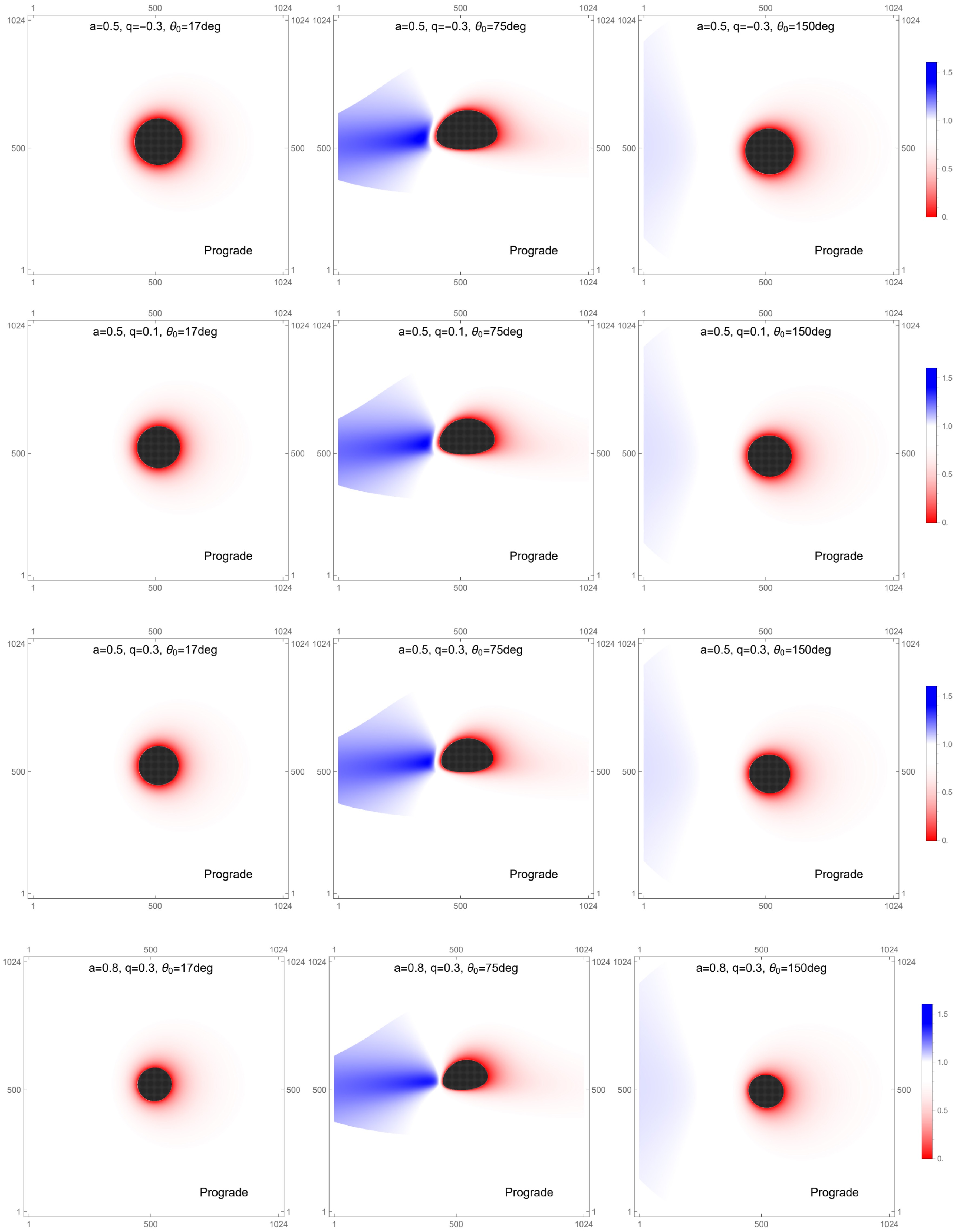
Figure 9. (color online) First-order frequency-shift images of prograde accretion disks. The panels show the frequency-shift distributions for different black hole parameter sets and observer inclination angles. The four parameter sets are
$ a=0.5 $ ,$ q=-0.3 $ ;$ a=0.5 $ ,$ q=0.1 $ ;$ a=0.5 $ ,$ q=0.3 $ ; and$ a=0.8 $ ,$ q=0.3 $ . For each case, the frequency-shift distribution is shown at observer inclination angles of$ 17^\circ $ ,$ 75^\circ $ , and$ 150^\circ $ . In all panels, the black hole mass is fixed at$ M=1 $ .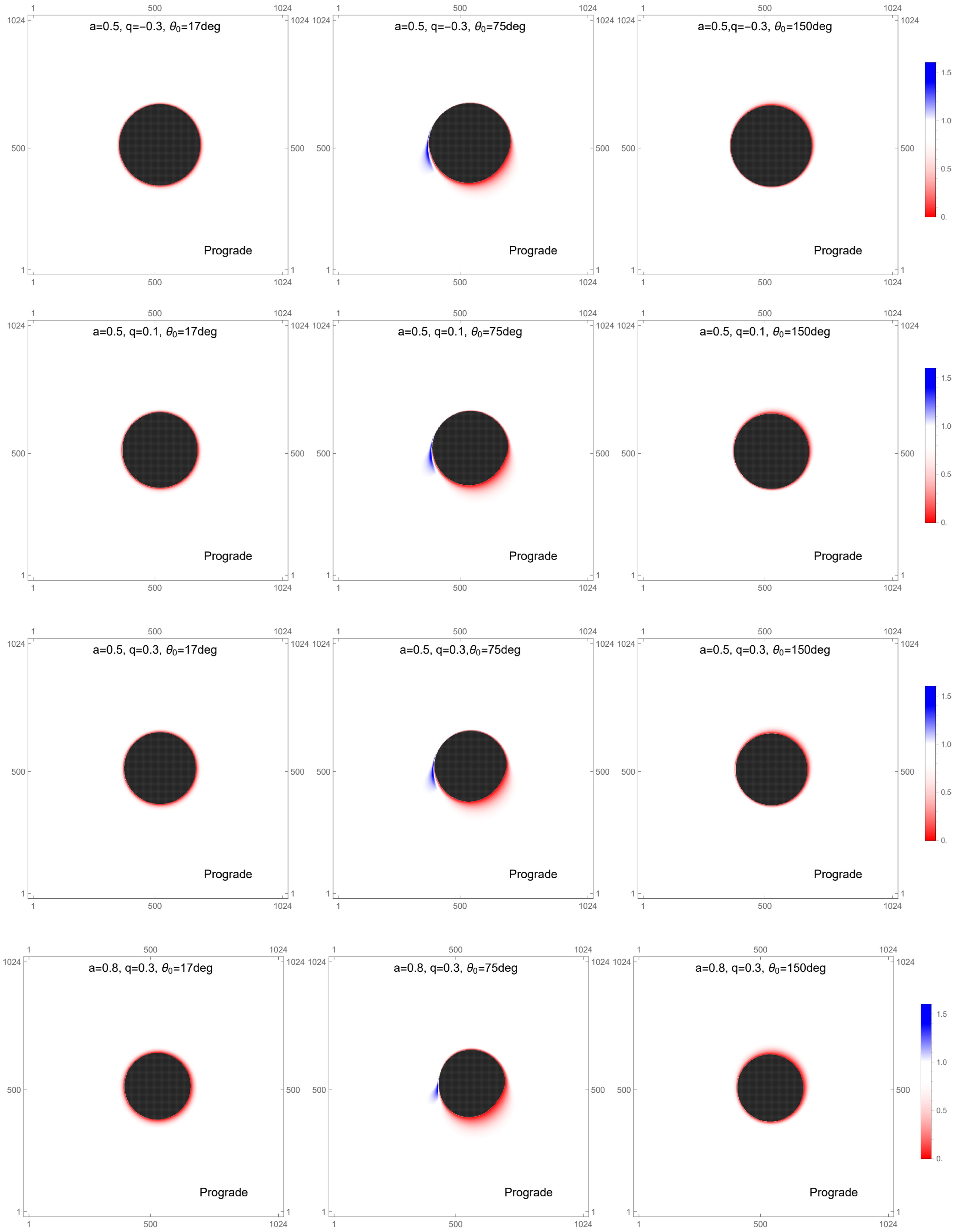
Figure 10. (color online) Second-order frequency-shift images for prograde accretion disks. The panels show the frequency-shift distribution for different black-hole parameter sets and observer inclination angles. The four parameter sets are
$ a=0.5 $ ,$ q=-0.3 $ ;$ a=0.5 $ ,$ q=0.1 $ ;$ a=0.5 $ ,$ q=0.3 $ ; and$ a=0.8 $ ,$ q=0.3 $ . For each case, the frequency-shift distribution is shown at observer inclination angles of$ 17^\circ $ ,$ 75^\circ $ , and$ 150^\circ $ . In all panels, the black-hole mass is fixed at$ M=1 $ .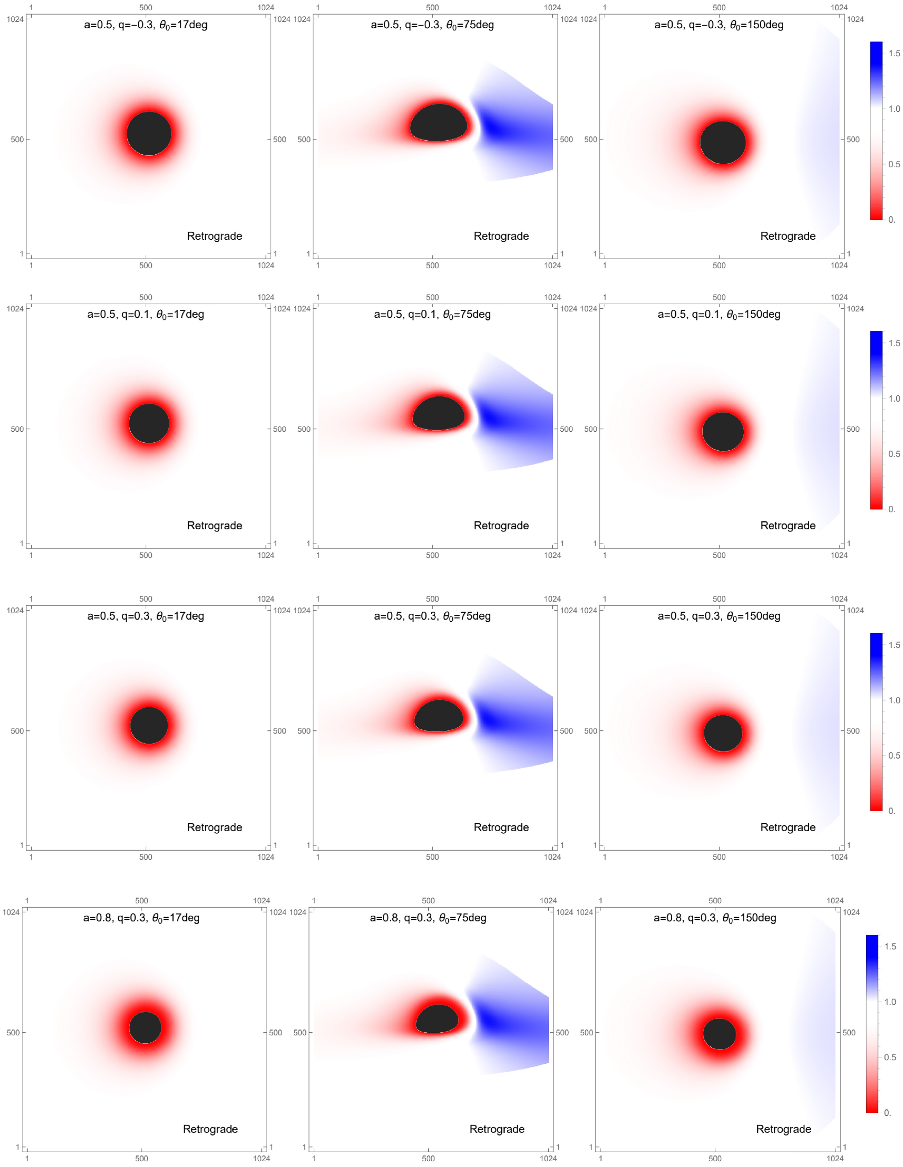
Figure 11. (color online) First-order frequency-shift images of retrograde accretion disks. The panels show the frequency-shift distribution for different black hole parameter sets and observer inclination angles. The four parameter sets are
$ a=0.5 $ ,$ q=-0.3 $ ;$ a=0.5 $ ,$ q=0.1 $ ;$ a=0.5 $ ,$ q=0.3 $ ; and$ a=0.8 $ ,$ q=0.3 $ . For each case, the frequency-shift distribution is shown for observer inclination angles of$ 17^\circ $ ,$ 75^\circ $ , and$ 150^\circ $ . In all panels, the black hole mass is fixed at$ M=1 $ .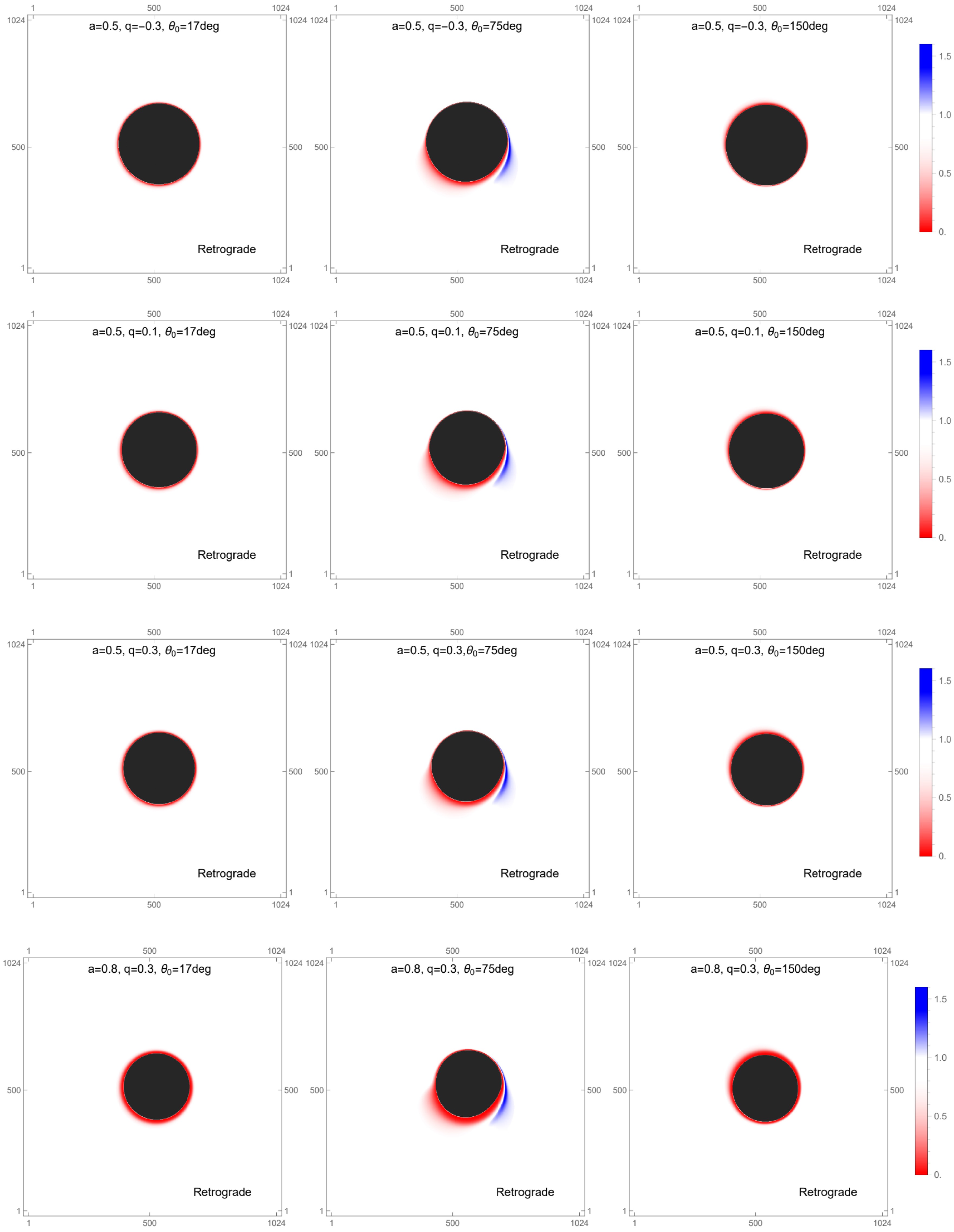
Figure 12. (color online) Second-order frequency-shift images of retrograde accretion disks. The panels show the frequency-shift distribution for different black hole parameter sets and observer inclination angles. The four parameter sets are
$ a=0.5 $ ,$ q=-0.3 $ ;$ a=0.5 $ ,$ q=0.1 $ ;$ a=0.5 $ ,$ q=0.3 $ ; and$ a=0.8 $ ,$ q=0.3 $ . For each case, the frequency-shift distribution is shown at observer inclination angles of$ 17^\circ $ ,$ 75^\circ $ , and$ 150^\circ $ . In all panels, the black hole mass is fixed at$ M=1 $ .This trend is mainly governed by the competition between kinematic Doppler boosting and gravitational redshift. When
$ \theta_0 $ is close to$ 0^\circ $ or$ 180^\circ $ , corresponding to a face-on view, the disk rotational velocity is nearly perpendicular to the line of sight. The line-of-sight velocity component is then very small, so the observed emission is dominated by gravitational redshift and transverse Doppler redshift, and the observable region remains strongly redshifted. When$ \theta_0 $ approaches$ 90^\circ $ , corresponding to an edge-on view, the projected rotational velocity becomes maximal. On the side of the disk moving toward the observer, the approaching velocity produces a strong Doppler blueshift that can overcome the gravitational redshift and enlarge the blueshifted region on the image plane. As$ \theta_0 $ continues toward$ 180^\circ $ , the line-of-sight velocity component decreases, the Doppler blueshift weakens, and gravitational redshift again becomes dominant.The same figures also demonstrate how the frequency-shift pattern responds to changes in the tidal charge and spin. Increasing the spin generally moves the ISCO inward, so that radiation can be emitted from regions closer to the event horizon, where gravitational redshift is stronger. A larger tidal charge produces a similar tendency and can also enhance the gravitational redshift. Even so, the location and amplitude of the peak blueshift change only weakly with a and q, especially when compared with the strong dependence on the observer inclination. Thus, the overall frequency-shift distribution is controlled mainly by the viewing angle, while the black hole spin and tidal charge provide secondary corrections.
Table 2 lists the maximum observed frequency-shift factors for rotating braneworld black holes with different spin parameters a, tidal charges q, disk rotation directions, and observer inclination angles. The row for
$ q=0 $ corresponds to the Kerr limit. According to the definition$ g=\nu_{\rm{obs}}/\nu_{\rm{em}} $ , values greater than unity indicate blueshift. The results show that the prograde disk generally attains a higher maximum frequency-shift factor than the retrograde disk, especially for$ \theta_0=75^\circ $ , whereas the dependence on q is relatively weak for$ \theta_0=150^\circ $ .a q Prograde Retrograde $ \theta_0=75^\circ $ $ \theta_0=150^\circ $ $ \theta_0=75^\circ $ $ \theta_0=150^\circ $ 0.5 $ -0.3 $ 1.53636 1.04895 1.48647 1.04801 0.5 0 1.53347 1.04889 1.48111 1.048 0.5 0.1 1.53439 1.04886 1.47871 1.04799 0.5 0.3 1.52399 1.04881 1.47662 1.04797 0.8 0.3 1.51033 1.04911 1.46542 1.04766 Table 2. Maximum observed frequency-shift factor for braneworld black holes with different parameter values. The row with
$ q=0 $ corresponds to the Kerr limit.Figures 13 and 14 show how the frequency-shift factor varies with the tidal charge and spin parameter. At fixed spin, the maximum frequency-shift factor decreases slightly as the tidal charge increases in both the prograde and retrograde cases, although the variation is small. At fixed tidal charge, it increases with spin for prograde motion but decreases for retrograde motion. Overall, the frequency-shift factor depends only weakly on the tidal charge and spin parameter, whereas the observer inclination remains the dominant factor.
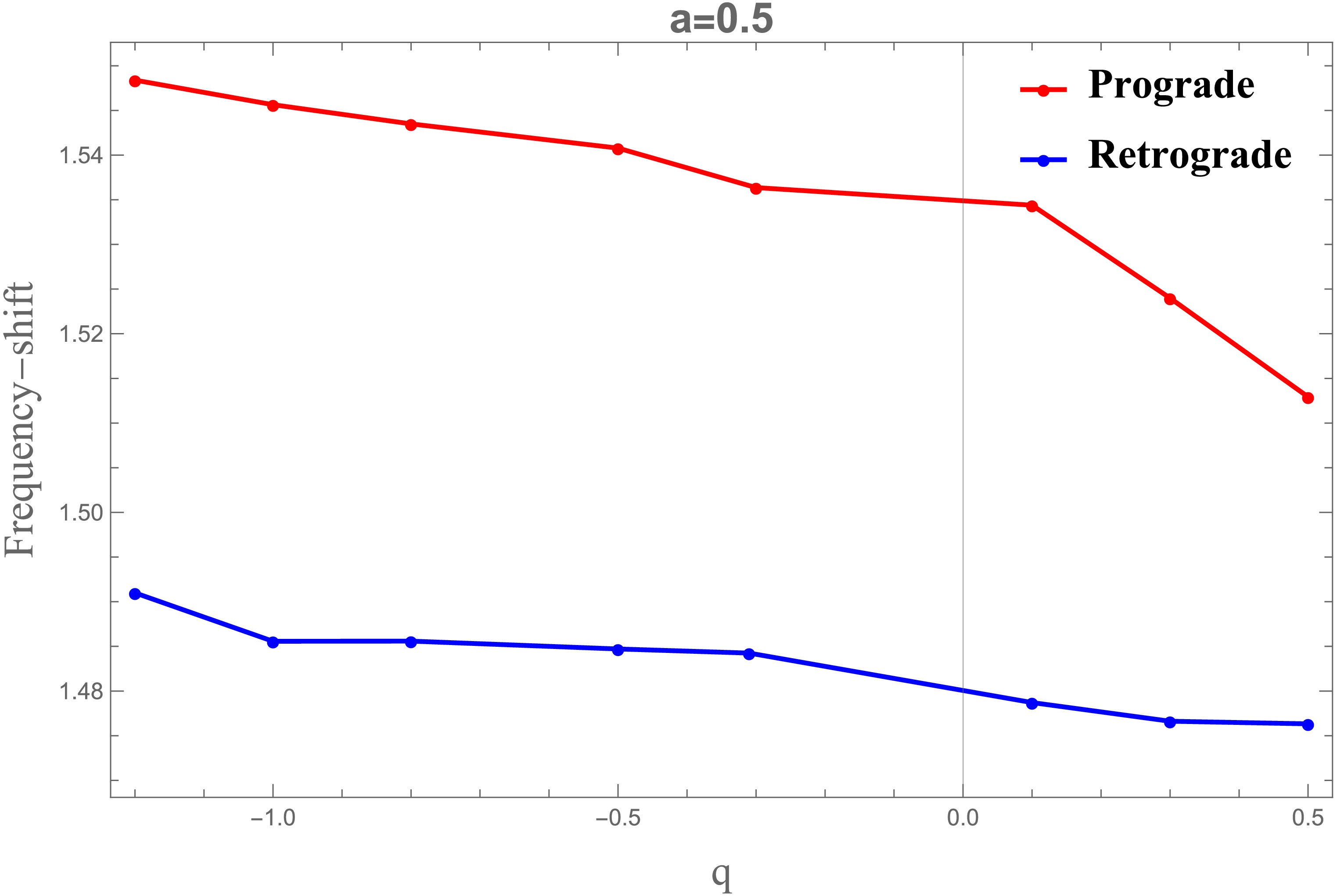
Figure 13. (color online) Blueshift profiles are shown for a fixed spin parameter
$ a=0.5 $ , with the tidal charge q varying over the range$ [-1.2,\,0.5] $ . In all panels, the black hole mass is set to$ M=1 $ .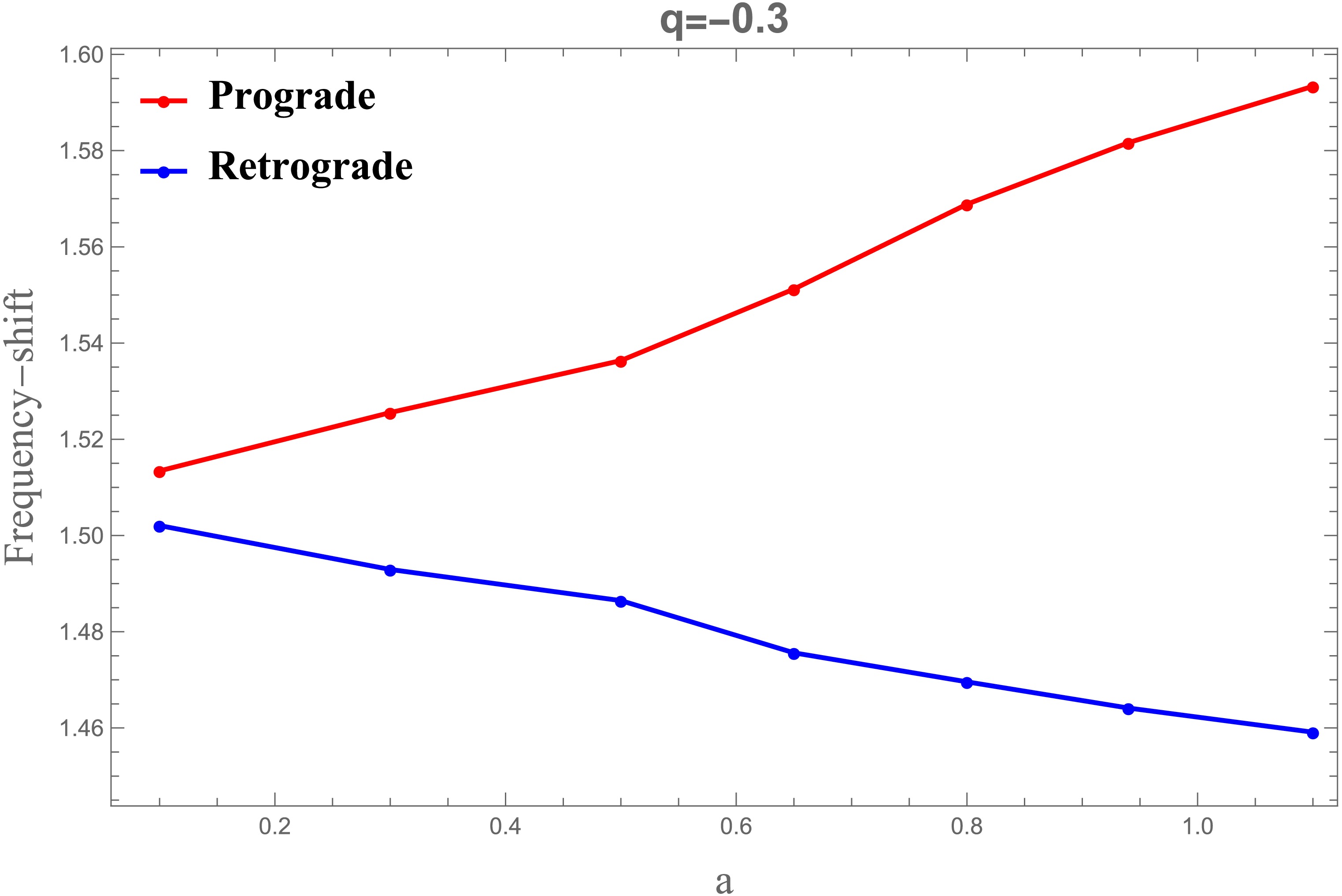
Figure 14. (color online) Blueshift profiles are shown for a fixed tidal charge
$ q=-0.3 $ , with the spin parameter a varying over the range$ [0.1,\,1.1] $ . In all panels, the black hole mass is set to$ M=1 $ . -
When analyzing photons emitted from the accretion disk that reach the observer’s image plane, it is essential to account for variations in the observed intensity due to scattering, absorption, Doppler boosting, and gravitational redshift. With these effects included, the radiative transfer equation governs the intensity measured by the observer [43]:
$ \frac{{\rm d}}{{\rm d}\lambda}\left(\frac{I_\nu}{\nu^3}\right) = \frac{J_\nu - \kappa_\nu I_\nu}{\nu^2}, $
(55) Here, λ is the affine parameter, while
$ I_{\nu} $ ,$ J_{\nu} $ , and$ \kappa_{\nu} $ denote the specific intensity, emission coefficient, and absorption coefficient at frequency ν, respectively. In vacuum,$ J_{\nu} $ and$ \kappa_{\nu} $ vanish; thus,$ I_{\nu}/\nu^{3} $ is conserved along the geodesic. Under the assumption that the accretion disk is geometrically and optically thin, the intensity profile on the observer’s image plane is obtained by integrating the photon trajectories. The observed intensity is therefore [12]$ I_{\nu_0} = \sum\limits_{m=1}^{N_{\rm{max}}} \left(\frac{\nu_0}{\nu_m}\right)^3 J_m \, \frac{1 - {\rm e}^{-\kappa_m \tau_{m-1}}}{\kappa_m}\, . $
(56) Here,
$ \nu_{0} $ denotes the photon frequency on the observer’s image plane,$ \nu_{m} $ denotes the frequency measured in the disk comoving frame, and$ \tau_{k} $ is the optical depth for photons emitted at point k. Accounting for the physical properties of the accretion disk, Eq. (56) can be simplified to$ I_{\nu_0} = \sum\limits_{m=1}^{N_{\max}} f_m \, g^3(r_m) \, J_{\rm model}(r_m), $
(57) where
$ f_{m} $ denotes a weighting factor,$ g(r_{m}) $ is the frequency-shift factor, and$J_{\rm model}(r_{m})$ represents the emissivity model evaluated at the emission radius$ r_{m} $ .In the following, we consider radiation emitted from the equatorial plane. For each image-plane coordinate
$ (\alpha,\beta) $ ,$ N_{\max}(\alpha,\beta) $ gives the number of intersections between the photon geodesic and the equatorial plane. For$ N_{\max}=1 $ , the geodesic crosses the equatorial plane only once, producing a direct image of the equatorial emission. For$ N_{\max}=2,3,4,\ldots $ multiple intersections occur, producing lensed and higher-order images.The radius
$ r_{m}(\alpha,\beta) $ is the radial position at which the geodesic associated with$ (\alpha,\beta) $ crosses the equatorial plane. Thus, the image order is determined by the number of equatorial-plane intersections rather than by the number of radial or angular turning points.In Eq. (57),
$J_{\rm model}(r_{m})$ is the emissivity evaluated at the emission radius$ r_{m} $ on the equatorial plane, g is the combined gravitational and Doppler frequency-shift factor, and$ f_{m} $ is a correction factor that adjusts the luminosity contribution from higher-order photon-ring images [39]. For the geometrically thin and optically thin disk considered here, we set$ f_{m}=1.5 $ throughout the analysis. The emissivity profile$J_{\rm model}(r)$ is modeled as [15]$ \log[J_{\rm model}(r)] = A \, \log \left(\frac{r}{r_H}\right) + B \left[\log \left(\frac{r}{r_H}\right)\right]^2, $
(58) where A and B are model-dependent fitting parameters, and
$ r_{H} $ denotes the black hole event horizon radius.At 230 GHz, the corresponding observing wavelength for M87
$ ^{*} $ and Sgr A$ ^{*} $ is 1.3 mm. We adopt$ A=-2 $ and$ B=-{1}/{2} $ at this frequency. At 86 GHz, we set$ A=0 $ and$ B=-{3}/{4} $ [15]. Using these values, we calculate the luminosity of the braneworld black hole within the thin-disk model. Figure 8 presents a comparison of the frequency at 230 GHz and 86 GHz.
Figure 8. (color online) Comparison of the accretion-disk emissivity profiles at 230 GHz and 86 GHz, with the event horizon radius fixed at
$ r_{H}=1 $ . In all cases, the black hole mass is set to$ M=1 $ .The frequency-shift factor is defined as
$ g=\nu_{0}/\nu_{m} $ . The disk model used here extends previous models by allowing radiation from the disk’s inner edge to reach the event horizon, thereby enabling a more detailed analysis of frequency-shift effects. Outside the ISCO, the accretion flow remains on circular orbits with angular velocity$ \Omega_{m}(r)=\left.\dfrac{u^{\phi}}{u^{t}}\right|_{r=r_{m}} $ .The parameter ξ is defined in Eq. (7), whereas ϵ measures the ratio of the observed energy to the conserved energy along the geodesic [12]:
$ \epsilon = \frac{E_0}{{\cal{E}}} = \frac{P_t}{k_t} = \delta \,(1 + \xi \chi). $
(59) The quantities χ and δ are defined in Eq. (51). Because the spacetime is asymptotically flat,
$ \epsilon=1 $ . For an emission radius$ r_{m} $ outside the ISCO, the frequency-shift factor therefore becomes [12]$ g_m = \frac{\epsilon}{\zeta \,(1 - \xi \Omega_m)}, \quad r_m \gt r_{\rm ISCO}, $
(60) where
$ \zeta = \sqrt{-\frac{1}{g_{tt} + 2 g_{t\phi} \Omega_m + g_{\phi\phi} \Omega_m^2}} \,\bigg|_{r = r_m}. $
(61) As discussed above, the ISCO determines the radial location of the inner boundary of the accretion disk. Inside the ISCO, the flow enters the plunging region and develops a radial velocity
$ u^{r}_{c} $ . In this region, the frequency-shift factor is$ g_m = \frac{\epsilon}{- \dfrac{u^r_c k_r}{k_t} + g^{tt} {\cal{E}}_{\rm{ISCO}} - \xi g^{t\phi} {\cal{E}}_{\rm{ISCO}} - g^{t\phi} {\cal{L}}_{\rm{ISCO}}+ \xi g^{\phi\phi} {\cal{L}}_{\rm{ISCO}}}. $
(62) For a clearer presentation of the frequency-shift distribution, the radial coordinate of the observer is set to
$ r_{o}=100R_{s} $ , where$ R_{s} $ is the Schwarzschild radius, and the image-plane angle is chosen as$ \phi=\pi/10 $ . Both prograde and retrograde disk rotations are included. Photons are classified according to whether they are emitted in the same direction as, or opposite to, the black hole rotation. This distinction is important because the direction of disk rotation strongly affects both the observed frequency shift and the photon trajectories near the braneworld black hole.Here, ''first-order'' and ''second-order'' refer to the number of intersections between a photon trajectory and the equatorial emitting plane, rather than to a perturbative expansion of the frequency-shift factor. The first-order map mainly represents the direct image, while the second-order map corresponds to the lensed image. Their comparison illustrates how stronger gravitational lensing modifies the observed frequency-shift distribution.
Figures 9–12 display the first- and second-order frequency-shift maps and show the kinematic imprint of the optically thin disk in both prograde and retrograde configurations. As the observer inclination
$ \theta_0 $ changes from$ 0^\circ $ toward$ 90^\circ $ , the redshifted area becomes smaller, while the blueshifted region expands. When$ \theta_0 $ increases further from$ 90^\circ $ to$ 180^\circ $ , the trend is reversed: the redshifted region grows again and the blueshifted area contracts.
Figure 9. (color online) First-order frequency-shift images of prograde accretion disks. The panels show the frequency-shift distributions for different black hole parameter sets and observer inclination angles. The four parameter sets are
$ a=0.5 $ ,$ q=-0.3 $ ;$ a=0.5 $ ,$ q=0.1 $ ;$ a=0.5 $ ,$ q=0.3 $ ; and$ a=0.8 $ ,$ q=0.3 $ . For each case, the frequency-shift distribution is shown at observer inclination angles of$ 17^\circ $ ,$ 75^\circ $ , and$ 150^\circ $ . In all panels, the black hole mass is fixed at$ M=1 $ .
Figure 10. (color online) Second-order frequency-shift images for prograde accretion disks. The panels show the frequency-shift distribution for different black-hole parameter sets and observer inclination angles. The four parameter sets are
$ a=0.5 $ ,$ q=-0.3 $ ;$ a=0.5 $ ,$ q=0.1 $ ;$ a=0.5 $ ,$ q=0.3 $ ; and$ a=0.8 $ ,$ q=0.3 $ . For each case, the frequency-shift distribution is shown at observer inclination angles of$ 17^\circ $ ,$ 75^\circ $ , and$ 150^\circ $ . In all panels, the black-hole mass is fixed at$ M=1 $ .
Figure 11. (color online) First-order frequency-shift images of retrograde accretion disks. The panels show the frequency-shift distribution for different black hole parameter sets and observer inclination angles. The four parameter sets are
$ a=0.5 $ ,$ q=-0.3 $ ;$ a=0.5 $ ,$ q=0.1 $ ;$ a=0.5 $ ,$ q=0.3 $ ; and$ a=0.8 $ ,$ q=0.3 $ . For each case, the frequency-shift distribution is shown for observer inclination angles of$ 17^\circ $ ,$ 75^\circ $ , and$ 150^\circ $ . In all panels, the black hole mass is fixed at$ M=1 $ .
Figure 12. (color online) Second-order frequency-shift images of retrograde accretion disks. The panels show the frequency-shift distribution for different black hole parameter sets and observer inclination angles. The four parameter sets are
$ a=0.5 $ ,$ q=-0.3 $ ;$ a=0.5 $ ,$ q=0.1 $ ;$ a=0.5 $ ,$ q=0.3 $ ; and$ a=0.8 $ ,$ q=0.3 $ . For each case, the frequency-shift distribution is shown at observer inclination angles of$ 17^\circ $ ,$ 75^\circ $ , and$ 150^\circ $ . In all panels, the black hole mass is fixed at$ M=1 $ .This trend is mainly governed by the competition between kinematic Doppler boosting and gravitational redshift. When
$ \theta_0 $ is close to$ 0^\circ $ or$ 180^\circ $ , corresponding to a face-on view, the disk rotational velocity is nearly perpendicular to the line of sight. The line-of-sight velocity component is then very small, so the observed emission is dominated by gravitational redshift and transverse Doppler redshift, and the observable region remains strongly redshifted. When$ \theta_0 $ approaches$ 90^\circ $ , corresponding to an edge-on view, the projected rotational velocity becomes maximal. On the side of the disk moving toward the observer, the approaching velocity produces a strong Doppler blueshift that can overcome the gravitational redshift and enlarge the blueshifted region on the image plane. As$ \theta_0 $ continues toward$ 180^\circ $ , the line-of-sight velocity component decreases, the Doppler blueshift weakens, and gravitational redshift again becomes dominant.The same figures also demonstrate how the frequency-shift pattern responds to changes in the tidal charge and spin. Increasing the spin generally moves the ISCO inward, so that radiation can be emitted from regions closer to the event horizon, where gravitational redshift is stronger. A larger tidal charge produces a similar tendency and can also enhance the gravitational redshift. Even so, the location and amplitude of the peak blueshift change only weakly with a and q, especially when compared with the strong dependence on the observer inclination. Thus, the overall frequency-shift distribution is controlled mainly by the viewing angle, while the black hole spin and tidal charge provide secondary corrections.
Table 2 lists the maximum observed frequency-shift factors for rotating braneworld black holes with different spin parameters a, tidal charges q, disk rotation directions, and observer inclination angles. The row for
$ q=0 $ corresponds to the Kerr limit. According to the definition$ g=\nu_{\rm{obs}}/\nu_{\rm{em}} $ , values greater than unity indicate blueshift. The results show that the prograde disk generally attains a higher maximum frequency-shift factor than the retrograde disk, especially for$ \theta_0=75^\circ $ , whereas the dependence on q is relatively weak for$ \theta_0=150^\circ $ .a q Prograde Retrograde $ \theta_0=75^\circ $ $ \theta_0=150^\circ $ $ \theta_0=75^\circ $ $ \theta_0=150^\circ $ 0.5 $ -0.3 $ 1.53636 1.04895 1.48647 1.04801 0.5 0 1.53347 1.04889 1.48111 1.048 0.5 0.1 1.53439 1.04886 1.47871 1.04799 0.5 0.3 1.52399 1.04881 1.47662 1.04797 0.8 0.3 1.51033 1.04911 1.46542 1.04766 Table 2. Maximum observed frequency-shift factor for braneworld black holes with different parameter values. The row with
$ q=0 $ corresponds to the Kerr limit.Figures 13 and 14 show how the frequency-shift factor varies with the tidal charge and spin parameter. At fixed spin, the maximum frequency-shift factor decreases slightly as the tidal charge increases in both the prograde and retrograde cases, although the variation is small. At fixed tidal charge, it increases with spin for prograde motion but decreases for retrograde motion. Overall, the frequency-shift factor depends only weakly on the tidal charge and spin parameter, whereas the observer inclination remains the dominant factor.
Figure 13. (color online) Blueshift profiles are shown for a fixed spin parameter
$ a=0.5 $ , with the tidal charge q varying over the range$ [-1.2,\,0.5] $ . In all panels, the black hole mass is set to$ M=1 $ .
Figure 14. (color online) Blueshift profiles are shown for a fixed tidal charge
$ q=-0.3 $ , with the spin parameter a varying over the range$ [0.1,\,1.1] $ . In all panels, the black hole mass is set to$ M=1 $ . -
We now simulate the apparent image of the braneworld black hole. Using Eq. (56) and a fish-eye camera ray-tracing technique, we generate synthetic images of a braneworld black hole illuminated by an optically thin accretion disk. At an observing frequency of 230 GHz, we adopt the phenomenological parameters
$ A=-2 $ and$ B=-1/2 $ , which specify the radial emissivity profile as follows:$ \log[J_{\rm model}(r)] = -2 \, \log \left(\frac{r}{r_H}\right) - \frac{1}{2}\left[\log \left(\frac{r}{r_H}\right)\right]^2 . $
(63) Figures 15 and 16 show the intensity profiles of the accretion disk along the x- and y-axes. The resulting trends are summarized as follows.
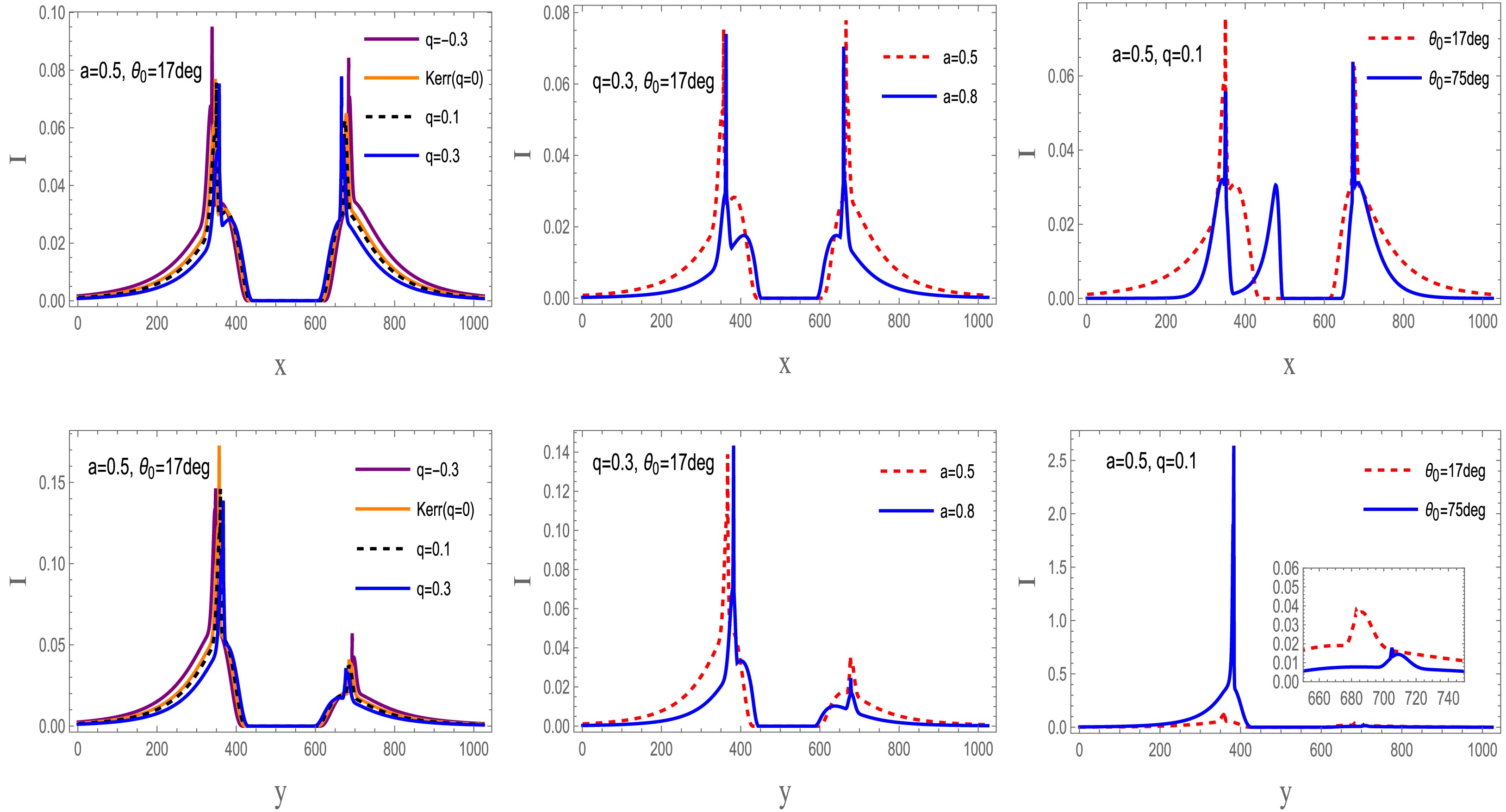
Figure 15. (color online) Intensity comparison for a prograde accretion disk. The 230 GHz intensity distribution of the braneworld black hole is shown. The first and second rows show slices along the x- and y-axes, respectively.
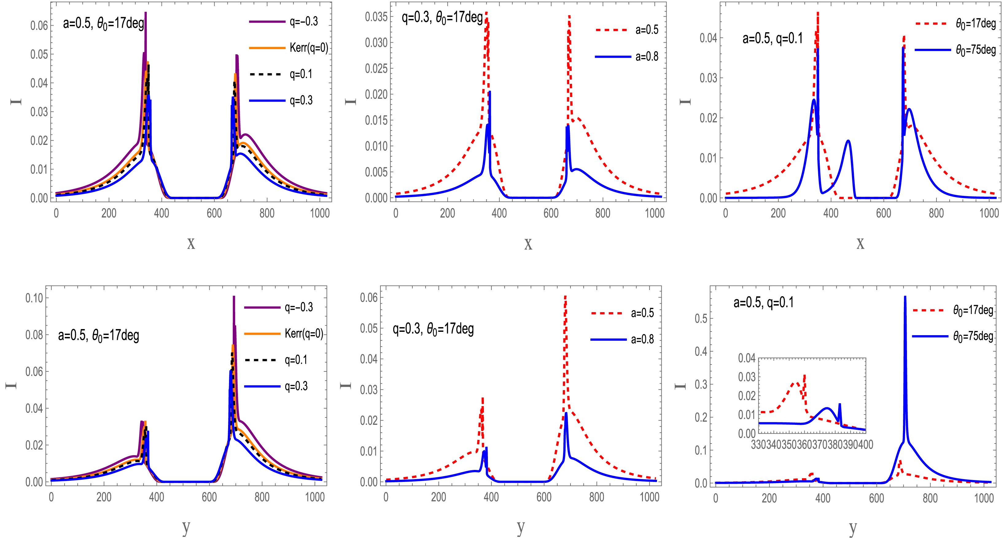
Figure 16. (color online) Comparison of the 230 GHz intensity profiles of a retrograde accretion disk around the braneworld black hole. The first and second rows show intensity slices along the x- and y-axes, respectively.
Along the x-axis, disk emission exhibits a clear dependence on the tidal charge, spin parameter, and observer inclination:
● Impact of the tidal charge: Regardless of the direction of disk rotation, the tidal charge has a consistent effect. In both prograde and retrograde configurations, the peak intensity increases as the tidal charge increases.
● Impact of the spin parameter: In contrast to the tidal charge, the spin parameter affects the prograde and retrograde configurations similarly, although the effect is more pronounced in the retrograde case. Increasing the spin parameter reduces the peak intensity, with stronger attenuation observed for retrograde accretion. Moreover, higher spin parameter values lead to an inward contraction of the central emitting region.
● Impact of the observer inclination: The observer inclination angle has an effect similar to that of the spin parameter. Regardless of the disk rotation direction, larger inclination angles progressively reduce the peak intensity while simultaneously driving an inward contraction of the central emitting region.
The emission characteristics along the y-axis differ significantly from those along the x-axis and exhibit distinct dependencies on the tidal charge, spin parameter, and observer inclination angle:
● Impact of the tidal charge: Regardless of the direction of disk rotation, the peak intensity decreases monotonically as the tidal charge increases. This suppression occurs in both prograde and retrograde configurations.
● Impact of the spin parameter: Unlike the tidal charge, the effect of the spin parameter depends on the accretion state. For a fixed tidal charge and observer inclination angle, increasing the spin parameter slightly enhances the peak intensity in the prograde case. In the retrograde case, however, the peak intensity decreases sharply with increasing spin and is accompanied by a pronounced inward contraction of the central emitting region.
● Impact of the observer inclination: The observer inclination angle exhibits a trend opposite to that observed along the x-axis. For both disk rotation directions, larger inclination angles significantly enhance the peak intensity, indicating a stronger angular dependence than that observed along the x-axis.
Figures 17 and 18 illustrate the apparent images of a braneworld black hole surrounded by an optically thin accretion disk for both prograde and retrograde accretion. Regardless of the disk rotation direction, for observer inclinations
$ \theta \lt \pi/2 $ , the morphological distinction between the direct and lensed images becomes increasingly pronounced as the inclination angle increases. At an observer inclination of$ \theta = 150^\circ $ , however, the overall intensity decreases, obscuring the boundary and making it substantially more difficult to distinguish the direct emission from the higher-order lensing rings.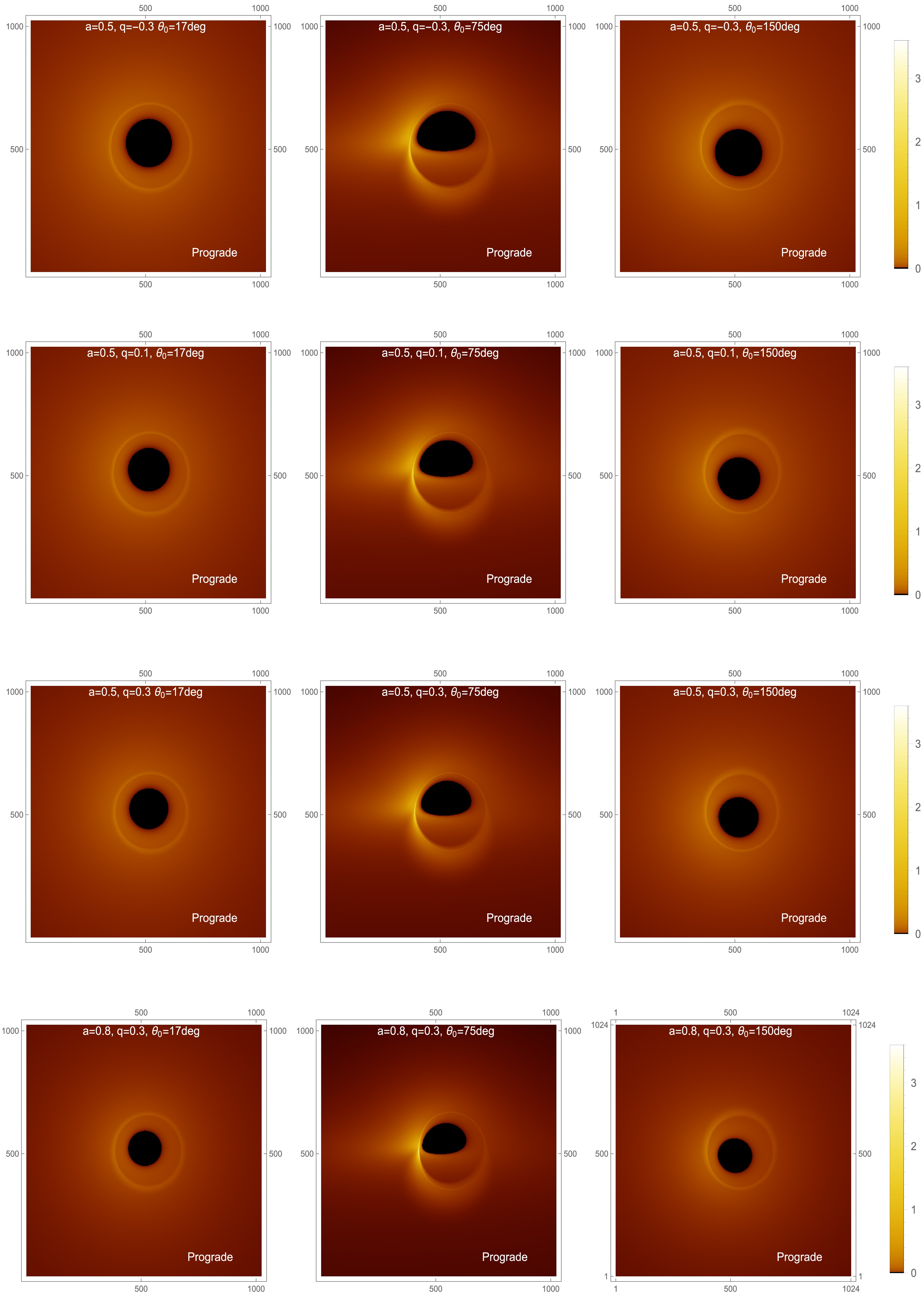
Figure 17. (color online) Intensity maps of the accretion disk in the prograde state at 230 GHz. The panels show the 230 GHz intensity distribution of the accretion disk for different black hole parameter sets and observer inclination angles. The four parameter sets are
$ a=0.5 $ ,$ q=-0.3 $ ;$ a=0.5 $ ,$ q=0.1 $ ;$ a=0.5 $ ,$ q=0.3 $ ; and$ a=0.8 $ ,$ q=0.3 $ . For each case, the intensity distribution is shown at observer inclination angles of$ 17^\circ $ ,$ 75^\circ $ , and$ 150^\circ $ . In all panels, the black hole mass is fixed at$ M=1 $ .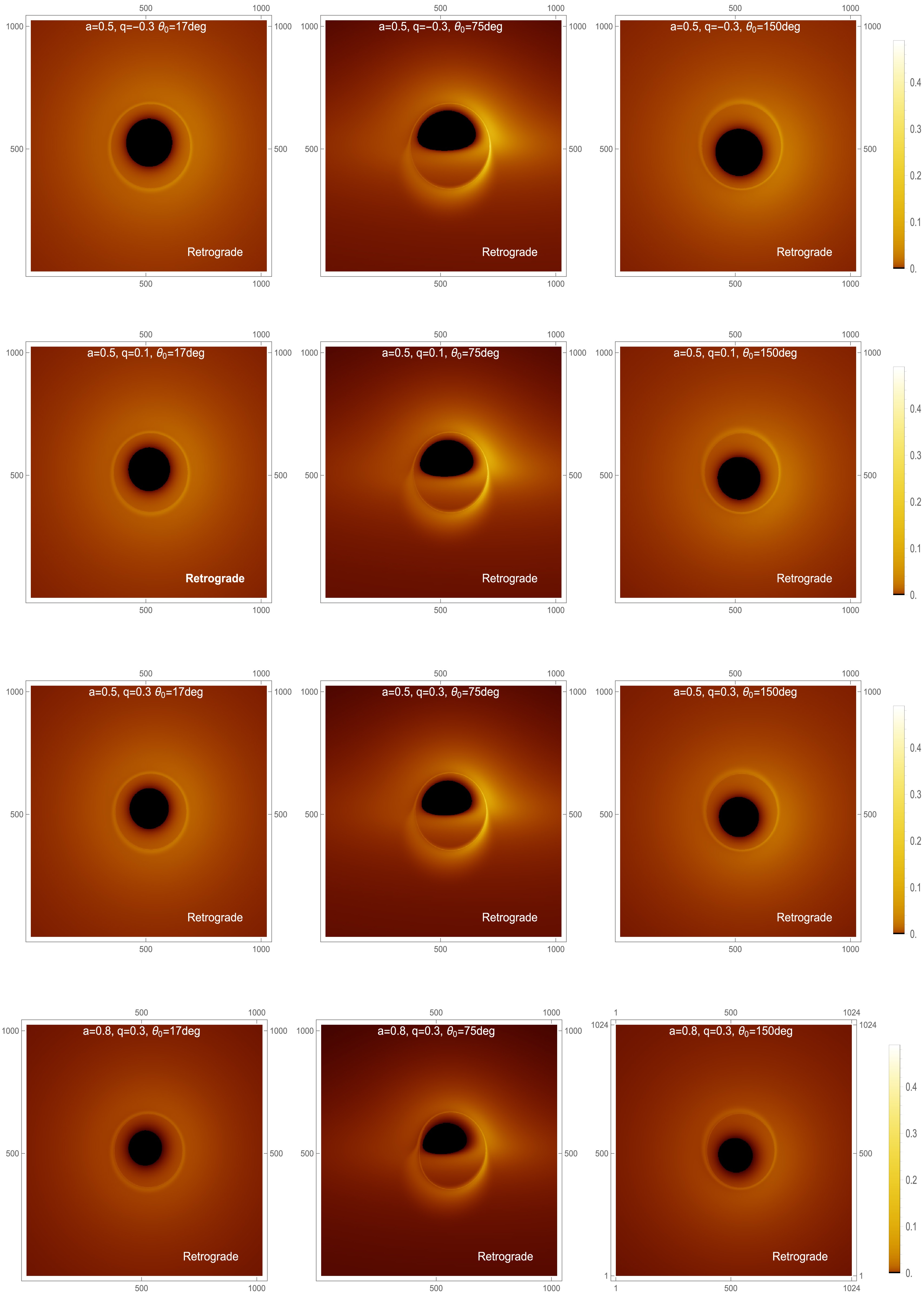
Figure 18. (color online) Intensity maps of the accretion disk in the retrograde state at 230 GHz. The panels show the 230 GHz intensity distribution of the accretion disk for different sets of black hole parameters and observer inclination angles. The four parameter sets are
$ a=0.5 $ ,$ q=-0.3 $ ;$ a=0.5 $ ,$ q=0.1 $ ;$ a=0.5 $ ,$ q=0.3 $ ; and$ a=0.8 $ ,$ q=0.3 $ . For each case, the intensity distribution is shown for observer inclination angles of$ 17^\circ $ ,$ 75^\circ $ , and$ 150^\circ $ . In all panels, the black hole mass is fixed at$ M=1 $ .Both the tidal charge and the spin parameter affect the shadow of the braneworld black hole, although the spin parameter is dominant. Nevertheless, the inner shadow and the critical curve remain detectable over a wide range of inclination angles, despite variations in the black hole spin and tidal charge, highlighting their fundamental nature in braneworld black hole spacetimes. The limited vertical extent of the accretion disk also reduces the central brightness in the simulated images. In addition, with sufficient angular resolution, the Doppler asymmetry induced by prograde and retrograde disk motion can be clearly identified on the image plane. For retrograde accretion, the Doppler signature is significantly stronger on the right-hand side of the image than on the opposite side. At the same time, frame dragging caused by the black hole spin produces an observable suppression of brightness in braneworld black hole images.
Figures 19 and 20 show how the intensity profiles depend on the tidal charge and spin. At fixed spin, the intensity increases steadily with the tidal charge in the prograde configuration but decreases in the retrograde configuration. At fixed tidal charge, a larger spin enhances the intensity for prograde accretion and suppresses it for retrograde accretion. Overall, the intensity variation is more pronounced in the prograde case than in the retrograde case, regardless of whether the spin or the tidal charge is varied. Thus, studying negative tidal charges in braneworld spacetime helps characterize how the tidal charge affects the frequency-shift behavior and radiation profiles in the present model.
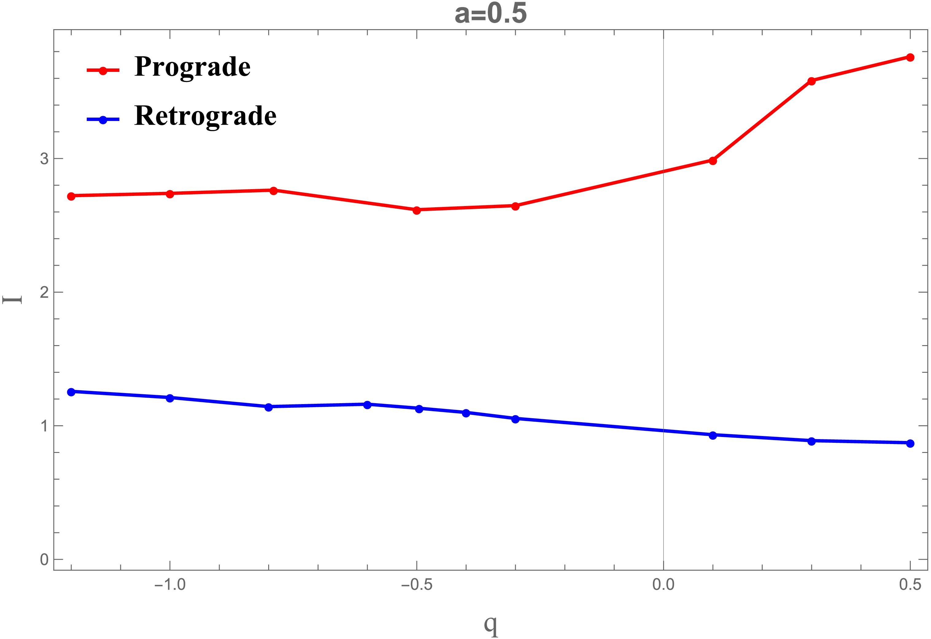
Figure 19. (color online) Intensity profiles are shown for a fixed spin parameter
$ a=0.5 $ , with the tidal charge q varying over the range$ [-1.2,\,0.5] $ . In all panels, the black hole mass is fixed at$ M=1 $ .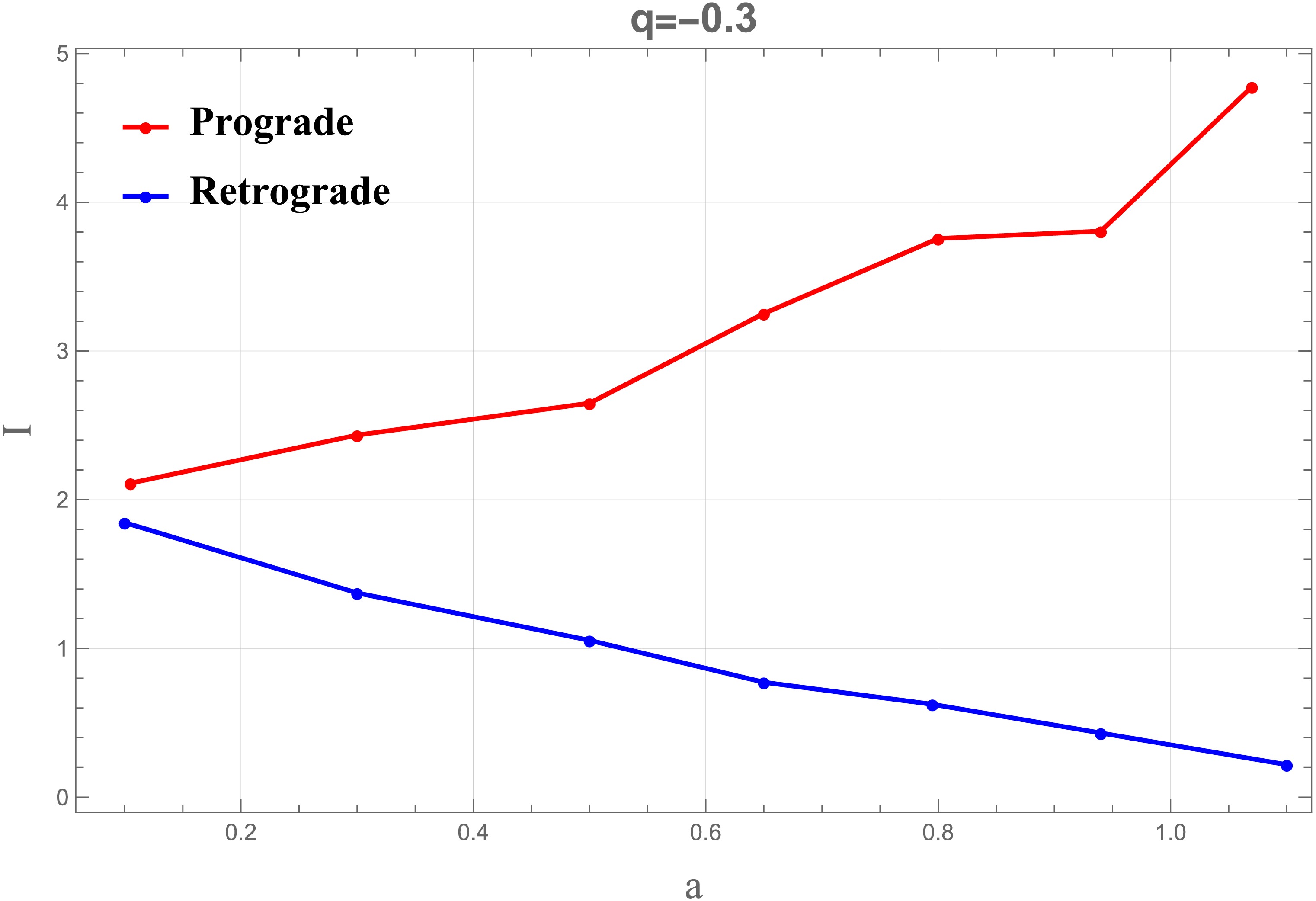
Figure 20. (color online) Intensity profiles for a fixed tidal charge of
$ q=-0.3 $ , with the spin parameter a varied over the range$ [0.1,\,1.1] $ . In all panels, the black hole mass is fixed at$ M=1 $ .Table 3 lists the maximum observed intensities for rotating braneworld black holes with different spin parameters a, tidal charges q, disk rotation directions, and observer inclination angles. The case
$ q=0 $ corresponds to the Kerr limit. The results show that prograde disks generally exhibit higher maximum observed intensities than retrograde disks, particularly for$ \theta_0=75^\circ $ . The maximum intensity also varies with the tidal charge q, indicating that the tidal charge affects the peak specific intensity on the observer’s image plane.a q Prograde Retrograde $ \theta_0=75^\circ $ $ \theta_0=150^\circ $ $ \theta_0=75^\circ $ $ \theta_0=150^\circ $ 0.5 $ -0.3 $ 2.64944 0.498447 1.05467 0.207229 0.5 0 2.80005 0.349915 1.28694 0.167148 0.5 0.1 2.98830 0.402825 0.93276 0.152894 0.5 0.3 3.58403 0.376889 0.88865 0.135587 0.8 0.3 3.38708 0.34138 0.26267 0.0527602 Table 3. Maximum observed intensity of braneworld black holes for different parameter values. The row with
$ q=0 $ corresponds to the Kerr limit.As a complement to the 230 GHz results, we also present 86 GHz images of a braneworld black hole with an optically thin accretion disk. At this frequency, we use
$ A=0 $ and$ B=-\dfrac{3}{4} $ , so that the emissivity profile is [15]:$ \log[J_{\rm model}(r)] = -\frac{3}{4}\left[\log \left(\frac{r}{r_H}\right)\right]^2. $
(64) Figures 21 and 22 present the 86 GHz intensity profiles of the accretion disk along the x- and y-axes. The main trends are as follows.
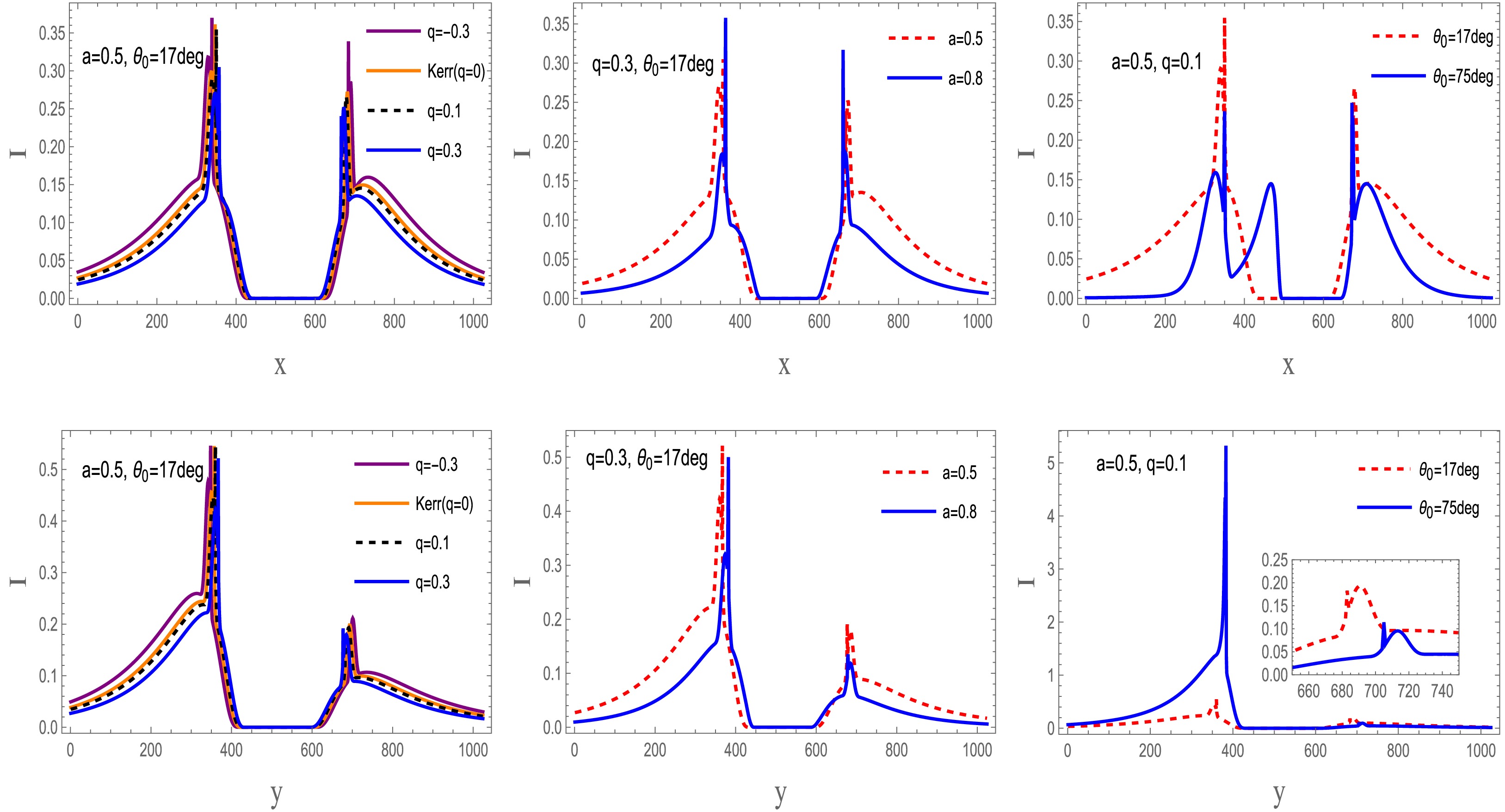
Figure 21. (color online) Comparison of 86 GHz intensity profiles for prograde accretion onto the braneworld black hole. The first and second rows show intensity cuts along the x- and y-axes, respectively.
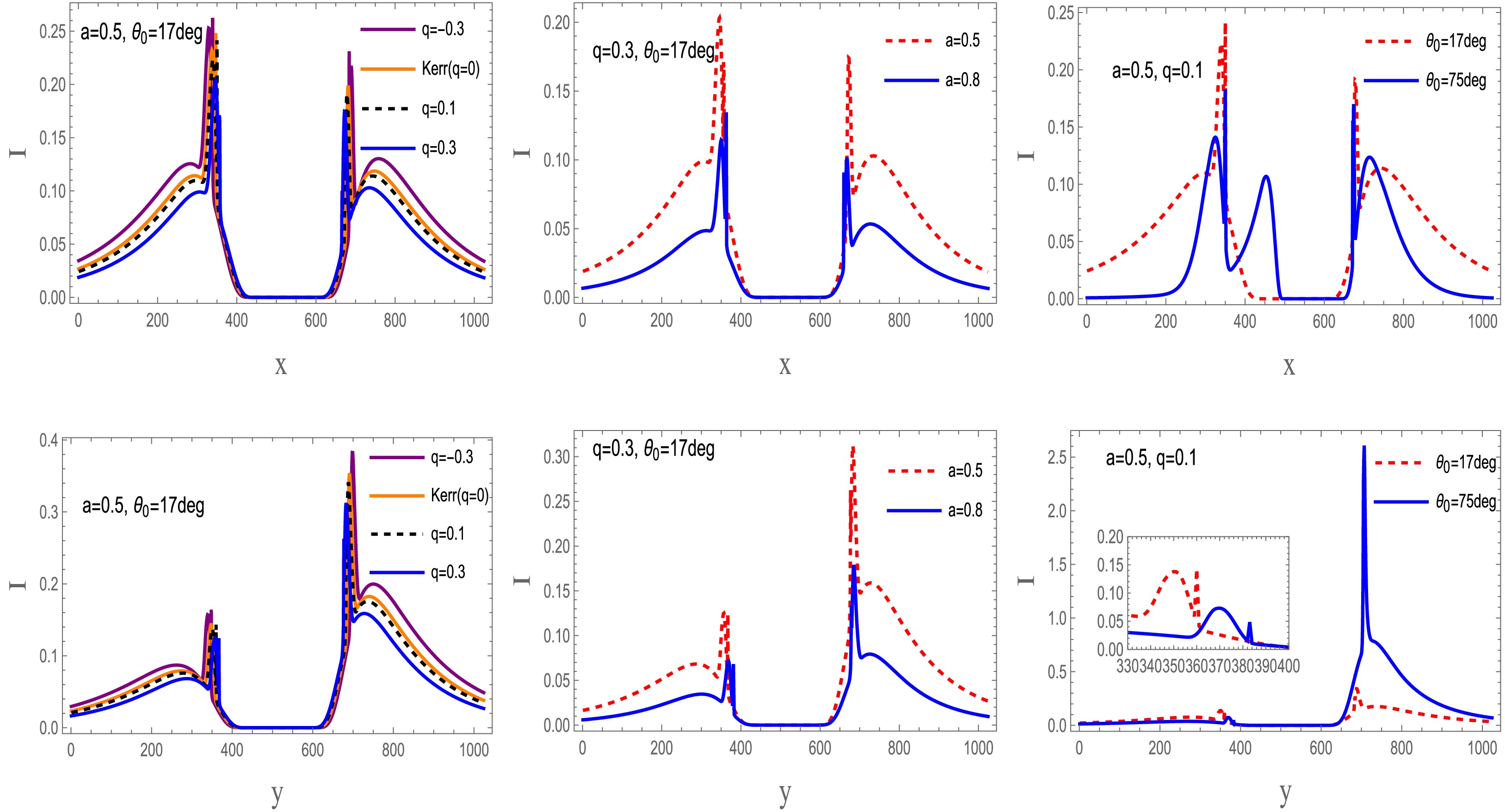
Figure 22. (color online) Comparison of the 86 GHz intensity profiles for retrograde accretion around a braneworld black hole. The first and second rows show intensity cuts along the x- and y-axes, respectively.
Along the x-axis, the emission characteristics of the accretion disk show distinct dependence on the spin parameter, tidal charge, and observer inclination angle:
● Impact of the spin parameter: The disk behavior differs significantly between the two accretion configurations. In prograde accretion, the peak intensity increases with spin, whereas in retrograde accretion, it decreases as the spin increases. Moreover, a larger spin parameter causes an inward contraction of the central high-intensity region.
● Impact of the tidal charge: As the tidal charge increases, the peak intensity gradually decreases in both prograde and retrograde configurations. This attenuation is more pronounced in the retrograde case.
● Impact of the observer inclination: The observer inclination angle induces a trend similar to that associated with the tidal charge. Irrespective of the disk rotation direction, the peak intensity decreases steadily as the observer inclination increases, and the central emitting region contracts inward.
The emission characteristics along the y-axis differ markedly from those along the x-axis and exhibit distinct dependencies on the same physical parameters:
● Impact of the spin parameter: When the tidal charge and inclination angle are held fixed, the effect of the spin parameter depends on the accretion configuration. In the prograde case, the peak intensity decreases as the spin parameter increases. In the retrograde case, this decrease is more pronounced and is accompanied by stronger inward contraction of the central emitting region.
● Impact of the tidal charge: Irrespective of the disk rotation direction, the peak intensity decreases steadily as the tidal charge increases.
● Impact of the observer inclination: The observer inclination angle exhibits a trend opposite to that found along the x-axis. For both prograde and retrograde configurations, the peak intensity increases significantly with increasing inclination angle, indicating a stronger angular dependence than that observed along the x-axis.
Figures 23 and 24 present the intensity images of the accretion disk in the prograde and retrograde cases at 86 GHz. Comparison of the 86 GHz and 230 GHz synthetic images reveals clear emission anisotropy between the profiles along the x- and y-axes. Nevertheless, the overall behavior remains consistent for both prograde and retrograde disks, and the 86 GHz images exhibit substantially higher total intensity. Across the image plane, the radiation intensity is strongly influenced by gravitational redshift and Doppler modulation. The central brightness depression associated with the inner shadow remains visible, and the critical curve is also preserved. These features suggest that, within the adopted disk model, the inner-shadow-like structure remains observable at both frequencies. However, this feature is not unique to braneworld black holes and should be interpreted in conjunction with the disk emissivity, observer inclination, and frequency-dependent radiative effects.
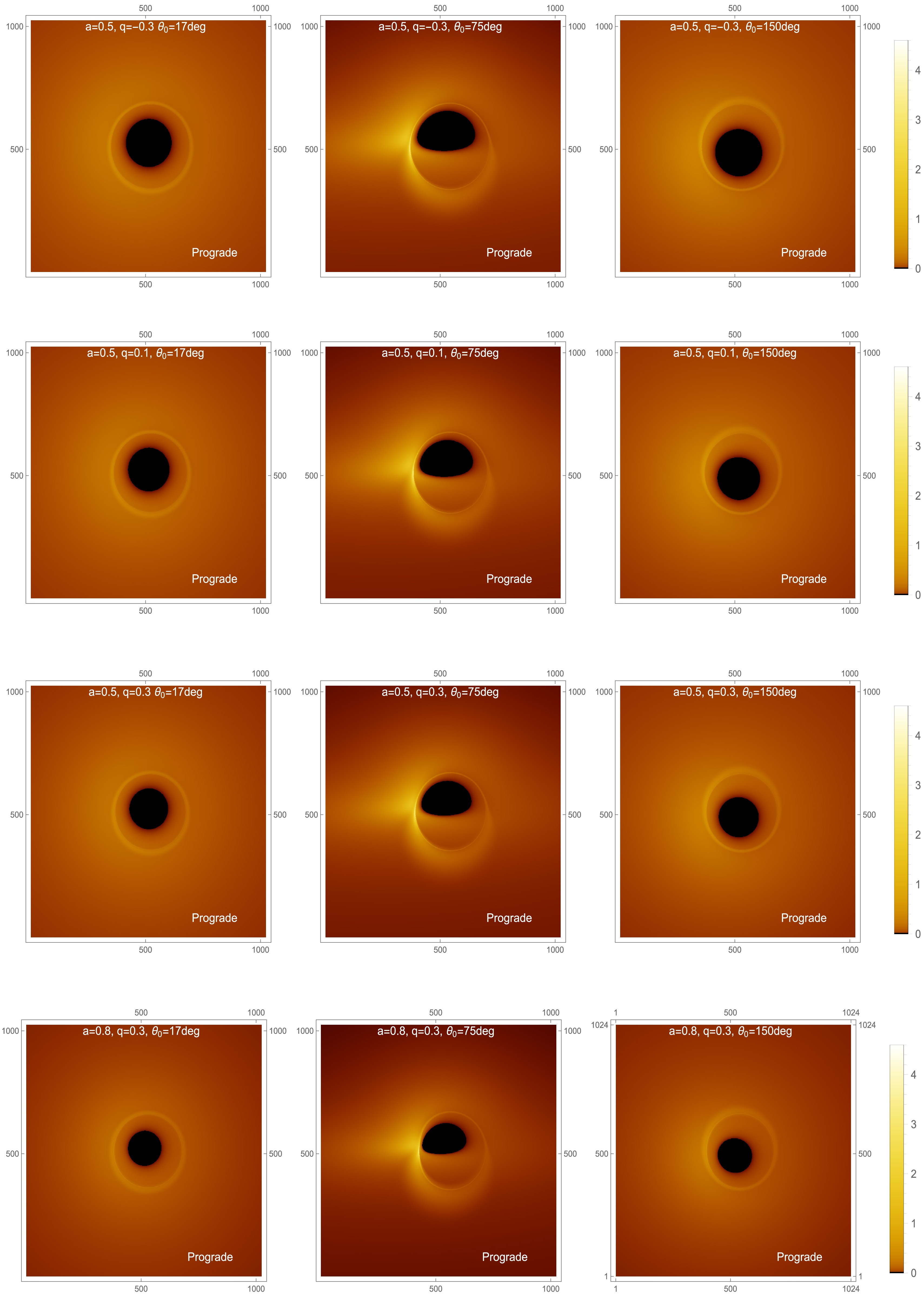
Figure 23. (color online) The 86 GHz intensity maps for a prograde accretion disk are shown. The panels present the 86 GHz intensity distributions for different black hole parameter sets and observer inclination angles. The four parameter sets considered are
$ a=0.5 $ ,$ q=-0.3 $ ;$ a=0.5 $ ,$ q=0.1 $ ;$ a=0.5 $ ,$ q=0.3 $ ; and$ a=0.8 $ ,$ q=0.3 $ . For each case, the intensity distribution is shown at observer inclination angles of$ 17^\circ $ ,$ 75^\circ $ , and$ 150^\circ $ . In all panels, the black hole mass is fixed at$ M=1 $ .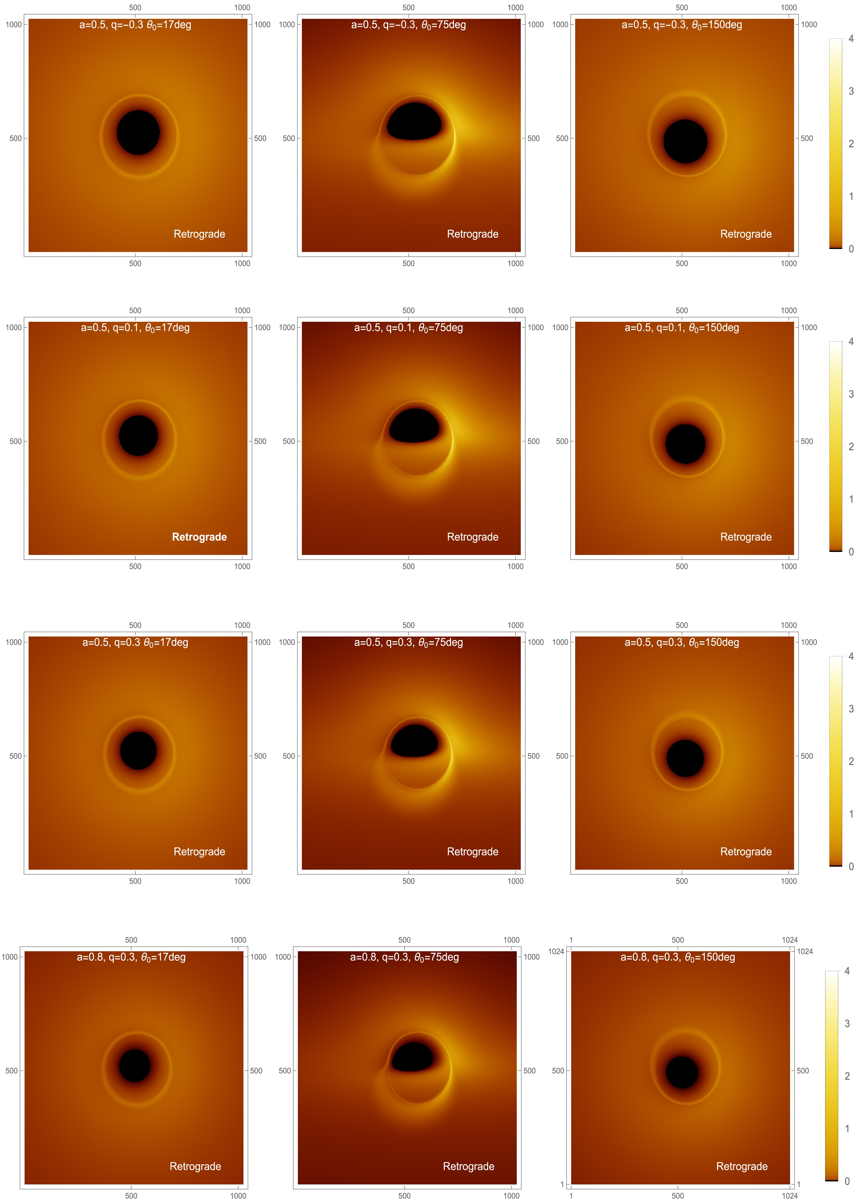
Figure 24. (color online) The 86 GHz intensity maps for a retrograde accretion disk are presented. The panels show the 86 GHz intensity distributions for different black hole parameter sets and observer inclination angles. The four parameter sets considered are
$ a=0.5 $ ,$ q=-0.3 $ ;$ a=0.5 $ ,$ q=0.1 $ ;$ a=0.5 $ ,$ q=0.3 $ ; and$ a=0.8 $ ,$ q=0.3 $ . For each parameter set, the intensity distribution is shown at observer inclination angles of$ 17^\circ $ ,$ 75^\circ $ , and$ 150^\circ $ . In all panels, the black hole mass is fixed at$ M=1 $ . -
We now simulate the apparent image of the braneworld black hole. Using Eq. (56) and a fish-eye camera ray-tracing technique, we generate synthetic images of a braneworld black hole illuminated by an optically thin accretion disk. At an observing frequency of 230 GHz, we adopt the phenomenological parameters
$ A=-2 $ and$ B=-1/2 $ , which specify the radial emissivity profile as follows:$ \log[J_{\rm model}(r)] = -2 \, \log \left(\frac{r}{r_H}\right) - \frac{1}{2}\left[\log \left(\frac{r}{r_H}\right)\right]^2 . $
(63) Figures 15 and 16 show the intensity profiles of the accretion disk along the x- and y-axes. The resulting trends are summarized as follows.
Figure 15. (color online) Intensity comparison for a prograde accretion disk. The 230 GHz intensity distribution of the braneworld black hole is shown. The first and second rows show slices along the x- and y-axes, respectively.
Figure 16. (color online) Comparison of the 230 GHz intensity profiles of a retrograde accretion disk around the braneworld black hole. The first and second rows show intensity slices along the x- and y-axes, respectively.
Along the x-axis, disk emission exhibits a clear dependence on the tidal charge, spin parameter, and observer inclination:
● Impact of the tidal charge: Regardless of the direction of disk rotation, the tidal charge has a consistent effect. In both prograde and retrograde configurations, the peak intensity increases as the tidal charge increases.
● Impact of the spin parameter: In contrast to the tidal charge, the spin parameter affects the prograde and retrograde configurations similarly, although the effect is more pronounced in the retrograde case. Increasing the spin parameter reduces the peak intensity, with stronger attenuation observed for retrograde accretion. Moreover, higher spin parameter values lead to an inward contraction of the central emitting region.
● Impact of the observer inclination: The observer inclination angle has an effect similar to that of the spin parameter. Regardless of the disk rotation direction, larger inclination angles progressively reduce the peak intensity while simultaneously driving an inward contraction of the central emitting region.
The emission characteristics along the y-axis differ significantly from those along the x-axis and exhibit distinct dependencies on the tidal charge, spin parameter, and observer inclination angle:
● Impact of the tidal charge: Regardless of the direction of disk rotation, the peak intensity decreases monotonically as the tidal charge increases. This suppression occurs in both prograde and retrograde configurations.
● Impact of the spin parameter: Unlike the tidal charge, the effect of the spin parameter depends on the accretion state. For a fixed tidal charge and observer inclination angle, increasing the spin parameter slightly enhances the peak intensity in the prograde case. In the retrograde case, however, the peak intensity decreases sharply with increasing spin and is accompanied by a pronounced inward contraction of the central emitting region.
● Impact of the observer inclination: The observer inclination angle exhibits a trend opposite to that observed along the x-axis. For both disk rotation directions, larger inclination angles significantly enhance the peak intensity, indicating a stronger angular dependence than that observed along the x-axis.
Figures 17 and 18 illustrate the apparent images of a braneworld black hole surrounded by an optically thin accretion disk for both prograde and retrograde accretion. Regardless of the disk rotation direction, for observer inclinations
$ \theta \lt \pi/2 $ , the morphological distinction between the direct and lensed images becomes increasingly pronounced as the inclination angle increases. At an observer inclination of$ \theta = 150^\circ $ , however, the overall intensity decreases, obscuring the boundary and making it substantially more difficult to distinguish the direct emission from the higher-order lensing rings.
Figure 17. (color online) Intensity maps of the accretion disk in the prograde state at 230 GHz. The panels show the 230 GHz intensity distribution of the accretion disk for different black hole parameter sets and observer inclination angles. The four parameter sets are
$ a=0.5 $ ,$ q=-0.3 $ ;$ a=0.5 $ ,$ q=0.1 $ ;$ a=0.5 $ ,$ q=0.3 $ ; and$ a=0.8 $ ,$ q=0.3 $ . For each case, the intensity distribution is shown at observer inclination angles of$ 17^\circ $ ,$ 75^\circ $ , and$ 150^\circ $ . In all panels, the black hole mass is fixed at$ M=1 $ .
Figure 18. (color online) Intensity maps of the accretion disk in the retrograde state at 230 GHz. The panels show the 230 GHz intensity distribution of the accretion disk for different sets of black hole parameters and observer inclination angles. The four parameter sets are
$ a=0.5 $ ,$ q=-0.3 $ ;$ a=0.5 $ ,$ q=0.1 $ ;$ a=0.5 $ ,$ q=0.3 $ ; and$ a=0.8 $ ,$ q=0.3 $ . For each case, the intensity distribution is shown for observer inclination angles of$ 17^\circ $ ,$ 75^\circ $ , and$ 150^\circ $ . In all panels, the black hole mass is fixed at$ M=1 $ .Both the tidal charge and the spin parameter affect the shadow of the braneworld black hole, although the spin parameter is dominant. Nevertheless, the inner shadow and the critical curve remain detectable over a wide range of inclination angles, despite variations in the black hole spin and tidal charge, highlighting their fundamental nature in braneworld black hole spacetimes. The limited vertical extent of the accretion disk also reduces the central brightness in the simulated images. In addition, with sufficient angular resolution, the Doppler asymmetry induced by prograde and retrograde disk motion can be clearly identified on the image plane. For retrograde accretion, the Doppler signature is significantly stronger on the right-hand side of the image than on the opposite side. At the same time, frame dragging caused by the black hole spin produces an observable suppression of brightness in braneworld black hole images.
Figures 19 and 20 show how the intensity profiles depend on the tidal charge and spin. At fixed spin, the intensity increases steadily with the tidal charge in the prograde configuration but decreases in the retrograde configuration. At fixed tidal charge, a larger spin enhances the intensity for prograde accretion and suppresses it for retrograde accretion. Overall, the intensity variation is more pronounced in the prograde case than in the retrograde case, regardless of whether the spin or the tidal charge is varied. Thus, studying negative tidal charges in braneworld spacetime helps characterize how the tidal charge affects the frequency-shift behavior and radiation profiles in the present model.
Figure 19. (color online) Intensity profiles are shown for a fixed spin parameter
$ a=0.5 $ , with the tidal charge q varying over the range$ [-1.2,\,0.5] $ . In all panels, the black hole mass is fixed at$ M=1 $ .
Figure 20. (color online) Intensity profiles for a fixed tidal charge of
$ q=-0.3 $ , with the spin parameter a varied over the range$ [0.1,\,1.1] $ . In all panels, the black hole mass is fixed at$ M=1 $ .Table 3 lists the maximum observed intensities for rotating braneworld black holes with different spin parameters a, tidal charges q, disk rotation directions, and observer inclination angles. The case
$ q=0 $ corresponds to the Kerr limit. The results show that prograde disks generally exhibit higher maximum observed intensities than retrograde disks, particularly for$ \theta_0=75^\circ $ . The maximum intensity also varies with the tidal charge q, indicating that the tidal charge affects the peak specific intensity on the observer’s image plane.a q Prograde Retrograde $ \theta_0=75^\circ $ $ \theta_0=150^\circ $ $ \theta_0=75^\circ $ $ \theta_0=150^\circ $ 0.5 $ -0.3 $ 2.64944 0.498447 1.05467 0.207229 0.5 0 2.80005 0.349915 1.28694 0.167148 0.5 0.1 2.98830 0.402825 0.93276 0.152894 0.5 0.3 3.58403 0.376889 0.88865 0.135587 0.8 0.3 3.38708 0.34138 0.26267 0.0527602 Table 3. Maximum observed intensity of braneworld black holes for different parameter values. The row with
$ q=0 $ corresponds to the Kerr limit.As a complement to the 230 GHz results, we also present 86 GHz images of a braneworld black hole with an optically thin accretion disk. At this frequency, we use
$ A=0 $ and$ B=-\dfrac{3}{4} $ , so that the emissivity profile is [15]:$ \log[J_{\rm model}(r)] = -\frac{3}{4}\left[\log \left(\frac{r}{r_H}\right)\right]^2. $
(64) Figures 21 and 22 present the 86 GHz intensity profiles of the accretion disk along the x- and y-axes. The main trends are as follows.
Figure 21. (color online) Comparison of 86 GHz intensity profiles for prograde accretion onto the braneworld black hole. The first and second rows show intensity cuts along the x- and y-axes, respectively.
Figure 22. (color online) Comparison of the 86 GHz intensity profiles for retrograde accretion around a braneworld black hole. The first and second rows show intensity cuts along the x- and y-axes, respectively.
Along the x-axis, the emission characteristics of the accretion disk show distinct dependence on the spin parameter, tidal charge, and observer inclination angle:
● Impact of the spin parameter: The disk behavior differs significantly between the two accretion configurations. In prograde accretion, the peak intensity increases with spin, whereas in retrograde accretion, it decreases as the spin increases. Moreover, a larger spin parameter causes an inward contraction of the central high-intensity region.
● Impact of the tidal charge: As the tidal charge increases, the peak intensity gradually decreases in both prograde and retrograde configurations. This attenuation is more pronounced in the retrograde case.
● Impact of the observer inclination: The observer inclination angle induces a trend similar to that associated with the tidal charge. Irrespective of the disk rotation direction, the peak intensity decreases steadily as the observer inclination increases, and the central emitting region contracts inward.
The emission characteristics along the y-axis differ markedly from those along the x-axis and exhibit distinct dependencies on the same physical parameters:
● Impact of the spin parameter: When the tidal charge and inclination angle are held fixed, the effect of the spin parameter depends on the accretion configuration. In the prograde case, the peak intensity decreases as the spin parameter increases. In the retrograde case, this decrease is more pronounced and is accompanied by stronger inward contraction of the central emitting region.
● Impact of the tidal charge: Irrespective of the disk rotation direction, the peak intensity decreases steadily as the tidal charge increases.
● Impact of the observer inclination: The observer inclination angle exhibits a trend opposite to that found along the x-axis. For both prograde and retrograde configurations, the peak intensity increases significantly with increasing inclination angle, indicating a stronger angular dependence than that observed along the x-axis.
Figures 23 and 24 present the intensity images of the accretion disk in the prograde and retrograde cases at 86 GHz. Comparison of the 86 GHz and 230 GHz synthetic images reveals clear emission anisotropy between the profiles along the x- and y-axes. Nevertheless, the overall behavior remains consistent for both prograde and retrograde disks, and the 86 GHz images exhibit substantially higher total intensity. Across the image plane, the radiation intensity is strongly influenced by gravitational redshift and Doppler modulation. The central brightness depression associated with the inner shadow remains visible, and the critical curve is also preserved. These features suggest that, within the adopted disk model, the inner-shadow-like structure remains observable at both frequencies. However, this feature is not unique to braneworld black holes and should be interpreted in conjunction with the disk emissivity, observer inclination, and frequency-dependent radiative effects.
Figure 23. (color online) The 86 GHz intensity maps for a prograde accretion disk are shown. The panels present the 86 GHz intensity distributions for different black hole parameter sets and observer inclination angles. The four parameter sets considered are
$ a=0.5 $ ,$ q=-0.3 $ ;$ a=0.5 $ ,$ q=0.1 $ ;$ a=0.5 $ ,$ q=0.3 $ ; and$ a=0.8 $ ,$ q=0.3 $ . For each case, the intensity distribution is shown at observer inclination angles of$ 17^\circ $ ,$ 75^\circ $ , and$ 150^\circ $ . In all panels, the black hole mass is fixed at$ M=1 $ .
Figure 24. (color online) The 86 GHz intensity maps for a retrograde accretion disk are presented. The panels show the 86 GHz intensity distributions for different black hole parameter sets and observer inclination angles. The four parameter sets considered are
$ a=0.5 $ ,$ q=-0.3 $ ;$ a=0.5 $ ,$ q=0.1 $ ;$ a=0.5 $ ,$ q=0.3 $ ; and$ a=0.8 $ ,$ q=0.3 $ . For each parameter set, the intensity distribution is shown at observer inclination angles of$ 17^\circ $ ,$ 75^\circ $ , and$ 150^\circ $ . In all panels, the black hole mass is fixed at$ M=1 $ . -
In this work, we conducted a systematic study of the observable properties of a braneworld black hole surrounded by an optically thin accretion disk. By combining ray tracing with a detailed analysis of photon trajectories, we investigated how the black hole image depends on the tidal charge and spin. The critical curve and inner shadow were determined using a quartic equation derived from the elliptic-integral description of photon motion. The results indicate that both a and q affect the deformation of the inner shadow, with the spin parameter producing the more pronounced distortion.
We also found that the observed intensity and frequency-shift distributions depend strongly on the observer inclination. This dependence is particularly evident near the ISCO, where the viewing angle largely determines the frequency-shift pattern. The frequency-shift asymmetry is generally more pronounced for prograde disks than for retrograde disks. In the prograde case, the left side of the image plane is blueshifted and the right side is redshifted, whereas this pattern is reversed for retrograde accretion.
We further compared the synthetic intensity distributions at 230 GHz and 86 GHz. The 86 GHz images exhibit both higher peak intensity and greater total intensity than the corresponding 230 GHz images. Nevertheless, the main spacetime-related structures, including the inner shadow and the critical curve, remain visible at both frequencies. This frequency dependence helps clarify the relationship between disk emission and photon-ring geometry and may provide useful theoretical guidance for future high-resolution black hole imaging studies.
Overall, our results show that the geometry of the accretion disk is crucial for determining the apparent image of a braneworld black hole, especially the photon ring and the inner shadow. Clear image asymmetries appear in both prograde and retrograde accretion cases because of the combined influence of spin, tidal charge, and viewing angle. These results provide a theoretical basis for future studies of high-resolution black hole images and may help characterize how the tidal charge modifies the apparent interaction between rotating braneworld black holes and their surrounding accretion flows.
-
In this work, we conducted a systematic study of the observable properties of a braneworld black hole surrounded by an optically thin accretion disk. By combining ray tracing with a detailed analysis of photon trajectories, we investigated how the black hole image depends on the tidal charge and spin. The critical curve and inner shadow were determined using a quartic equation derived from the elliptic-integral description of photon motion. The results indicate that both a and q affect the deformation of the inner shadow, with the spin parameter producing the more pronounced distortion.
We also found that the observed intensity and frequency-shift distributions depend strongly on the observer inclination. This dependence is particularly evident near the ISCO, where the viewing angle largely determines the frequency-shift pattern. The frequency-shift asymmetry is generally more pronounced for prograde disks than for retrograde disks. In the prograde case, the left side of the image plane is blueshifted and the right side is redshifted, whereas this pattern is reversed for retrograde accretion.
We further compared the synthetic intensity distributions at 230 GHz and 86 GHz. The 86 GHz images exhibit both higher peak intensity and greater total intensity than the corresponding 230 GHz images. Nevertheless, the main spacetime-related structures, including the inner shadow and the critical curve, remain visible at both frequencies. This frequency dependence helps clarify the relationship between disk emission and photon-ring geometry and may provide useful theoretical guidance for future high-resolution black hole imaging studies.
Overall, our results show that the geometry of the accretion disk is crucial for determining the apparent image of a braneworld black hole, especially the photon ring and the inner shadow. Clear image asymmetries appear in both prograde and retrograde accretion cases because of the combined influence of spin, tidal charge, and viewing angle. These results provide a theoretical basis for future studies of high-resolution black hole images and may help characterize how the tidal charge modifies the apparent interaction between rotating braneworld black holes and their surrounding accretion flows.
-
In this appendix, we present the detailed derivation of Eqs. (15)–(17). The corresponding radial and angular integrals are defined as
$ I_{t} = -\int\nolimits_{r_{s}}^{r_{o}} \frac{(2Mr - q)(a^{2} + r^{2} - a\xi) + \Delta(r)\,r^{2}} {\pm_{r}\,\Delta(r)\,\sqrt{{\cal{R}}(r)}}\,{\rm d}r, $
(A1) $ I_{\tau} = -\int\nolimits_{r_{s}}^{r_{o}} \frac{{\rm d}r}{\pm_{r}\,\sqrt{{\cal{R}}(r)}}, $
(A2) $ I_{\phi} = -\int\nolimits_{r_{s}}^{r_{o}} \frac{2aMr - a^{2}\xi - aq} {\pm_{r}\,\Delta(r)\,\sqrt{{\cal{R}}(r)}}\,{\rm d}r, $
(A3) $ G_{t} = -\int\nolimits_{\theta_{s}}^{\theta_{o}} \frac{\cos^{2}\theta}{\pm_{\theta}\,\sqrt{{\cal{B}}(\theta)}}\,{\rm d}\theta, $
(A4) $ G_{\theta} = -\int\nolimits_{\theta_{s}}^{\theta_{o}} \frac{{\rm d}\theta}{\pm_{\theta}\,\sqrt{\Theta(\theta)}}, $
(A5) $ G_{\phi} = -\int\nolimits_{\theta_{s}}^{\theta_{o}} \frac{\csc^{2}\theta}{\pm_{\theta}\,\sqrt{\Theta(\theta)}}\,{\rm d}\theta. $
(A6) -
In this appendix, we present the detailed derivation of Eqs. (15)–(17). The corresponding radial and angular integrals are defined as
$ I_{t} = -\int\nolimits_{r_{s}}^{r_{o}} \frac{(2Mr - q)(a^{2} + r^{2} - a\xi) + \Delta(r)\,r^{2}} {\pm_{r}\,\Delta(r)\,\sqrt{{\cal{R}}(r)}}\,{\rm d}r, $
(A1) $ I_{\tau} = -\int\nolimits_{r_{s}}^{r_{o}} \frac{{\rm d}r}{\pm_{r}\,\sqrt{{\cal{R}}(r)}}, $
(A2) $ I_{\phi} = -\int\nolimits_{r_{s}}^{r_{o}} \frac{2aMr - a^{2}\xi - aq} {\pm_{r}\,\Delta(r)\,\sqrt{{\cal{R}}(r)}}\,{\rm d}r, $
(A3) $ G_{t} = -\int\nolimits_{\theta_{s}}^{\theta_{o}} \frac{\cos^{2}\theta}{\pm_{\theta}\,\sqrt{{\cal{B}}(\theta)}}\,{\rm d}\theta, $
(A4) $ G_{\theta} = -\int\nolimits_{\theta_{s}}^{\theta_{o}} \frac{{\rm d}\theta}{\pm_{\theta}\,\sqrt{\Theta(\theta)}}, $
(A5) $ G_{\phi} = -\int\nolimits_{\theta_{s}}^{\theta_{o}} \frac{\csc^{2}\theta}{\pm_{\theta}\,\sqrt{\Theta(\theta)}}\,{\rm d}\theta. $
(A6) -
For massive particles in the accretion disk, we denote the conserved specific energy and angular momentum by
$ {\cal{E}}=-u_t,\qquad {\cal{L}}=u_\phi , $
(B1) where
$ u^\mu $ denotes the four-velocity of the disk matter. These quantities refer to timelike particles in the disk and should be distinguished from the photon constants of motion introduced in the previous section.The normalization condition for massive particles is
$ u^\mu u_\mu=-1 . $
(B2) Equivalently, it can be written as
$ g^{\mu\nu}u_\mu u_\nu=-1 . $
(B3) For equatorial motion,
$ \theta=\pi/2 $ and$ u^\theta=0 $ ; therefore, we have$ g^{tt}u_t^2+2g^{t\phi}u_tu_\phi +g^{\phi\phi}u_\phi^2+g^{rr}u_r^2=-1 . $
(B4) Substituting
$ u_t=-{\cal{E}} $ and$ u_\phi={\cal{L}} $ yields$ g^{tt}{\cal{E}}^2-2g^{t\phi}{\cal{E}}{\cal{L}} +g^{\phi\phi}{\cal{L}}^2+g^{rr}u_r^2=-1 . $
(B5) Therefore,
$ g^{rr}u_r^2 = -\left( 1+g^{tt}{\cal{E}}^2 -2g^{t\phi}{\cal{E}}{\cal{L}} +g^{\phi\phi}{\cal{L}}^2 \right). $
(B6) We then define the effective potential as
$ V(r,{\cal{E}},{\cal{L}})= \left( 1+g^{tt}{\cal{E}}^2 -2g^{t\phi}{\cal{E}}{\cal{L}} +g^{\phi\phi}{\cal{L}}^2 \right)_{\theta=\pi/2}. $
(B7) Thus,
$ g^{rr}u_r^2=-V(r,{\cal{E}},{\cal{L}}). $
(B8) Since the metric contains no r–t or r–ϕ cross terms, we have
$ g^{rr}=1/g_{rr} $ and$ u^r=g^{rr}u_r $ . Hence,$ (u^r)^2 = -g^{rr}V(r,{\cal{E}},{\cal{L}}) = -\frac{V(r,{\cal{E}},{\cal{L}})}{g_{rr}} . $
(B9) For the inward-plunging branch, we take the negative sign and obtain
$ u^r = -\sqrt{ -\frac{V(r,{\cal{E}},{\cal{L}})}{g_{rr}} }. $
(B10) The minus sign preceding the square root denotes inward radial motion. The allowed radial motion satisfies
$ V(r,{\cal{E}},{\cal{L}})\leqslant 0 $ , ensuring that the quantity under the square root is non-negative. -
For massive particles in the accretion disk, we denote the conserved specific energy and angular momentum by
$ {\cal{E}}=-u_t,\qquad {\cal{L}}=u_\phi , $
(B1) where
$ u^\mu $ denotes the four-velocity of the disk matter. These quantities refer to timelike particles in the disk and should be distinguished from the photon constants of motion introduced in the previous section.The normalization condition for massive particles is
$ u^\mu u_\mu=-1 . $
(B2) Equivalently, it can be written as
$ g^{\mu\nu}u_\mu u_\nu=-1 . $
(B3) For equatorial motion,
$ \theta=\pi/2 $ and$ u^\theta=0 $ ; therefore, we have$ g^{tt}u_t^2+2g^{t\phi}u_tu_\phi +g^{\phi\phi}u_\phi^2+g^{rr}u_r^2=-1 . $
(B4) Substituting
$ u_t=-{\cal{E}} $ and$ u_\phi={\cal{L}} $ yields$ g^{tt}{\cal{E}}^2-2g^{t\phi}{\cal{E}}{\cal{L}} +g^{\phi\phi}{\cal{L}}^2+g^{rr}u_r^2=-1 . $
(B5) Therefore,
$ g^{rr}u_r^2 = -\left( 1+g^{tt}{\cal{E}}^2 -2g^{t\phi}{\cal{E}}{\cal{L}} +g^{\phi\phi}{\cal{L}}^2 \right). $
(B6) We then define the effective potential as
$ V(r,{\cal{E}},{\cal{L}})= \left( 1+g^{tt}{\cal{E}}^2 -2g^{t\phi}{\cal{E}}{\cal{L}} +g^{\phi\phi}{\cal{L}}^2 \right)_{\theta=\pi/2}. $
(B7) Thus,
$ g^{rr}u_r^2=-V(r,{\cal{E}},{\cal{L}}). $
(B8) Since the metric contains no r–t or r–ϕ cross terms, we have
$ g^{rr}=1/g_{rr} $ and$ u^r=g^{rr}u_r $ . Hence,$ (u^r)^2 = -g^{rr}V(r,{\cal{E}},{\cal{L}}) = -\frac{V(r,{\cal{E}},{\cal{L}})}{g_{rr}} . $
(B9) For the inward-plunging branch, we take the negative sign and obtain
$ u^r = -\sqrt{ -\frac{V(r,{\cal{E}},{\cal{L}})}{g_{rr}} }. $
(B10) The minus sign preceding the square root denotes inward radial motion. The allowed radial motion satisfies
$ V(r,{\cal{E}},{\cal{L}})\leqslant 0 $ , ensuring that the quantity under the square root is non-negative. -
In this appendix, we derive the four-velocity of the plunging accretion flow inside the innermost stable circular orbit (ISCO) of a rotating braneworld black hole. For a massive particle, the conserved specific energy and specific angular momentum are defined as [44]
$ {\cal{E}}=-u_t, \qquad {\cal{L}}=u_\phi. $
(C1) In the equatorial plane,
$ \theta=\pi/2 $ , the metric function is$ \Delta=r^2-2Mr+a^2+q. $
(C2) Throughout this appendix, the upper and lower signs correspond to prograde and retrograde motion, respectively. For a given orbital branch, the same sign choice must be used consistently in all expressions.
The ISCO radius is determined by the marginal-stability condition
$ \begin{aligned}[b] & Mr_{\rm{ISCO}}^3 -6M^2r_{\rm{ISCO}}^2 +9Mqr_{\rm{ISCO}} -4q^2 +a^2\left(4q-3Mr_{\rm{ISCO}}\right) \\ & \pm 8a\left(Mr_{\rm{ISCO}}-q\right)^{3/2} =0. \end{aligned} $
(C3) The physically relevant root is selected to lie outside the outer event horizon and must satisfy
$ Mr_{\rm{ISCO}}-q\geqslant0, $
(C4) together with
$ r_{\rm{ISCO}}^2 -3Mr_{\rm{ISCO}} +2q \pm 2a\sqrt{Mr_{\rm{ISCO}}-q} >0. $
(C5) Within the ISCO, stable circular motion is no longer possible. Following Cunningham’s prescription, we assume that the plunging matter retains the conserved specific energy and angular momentum of the circular orbit at the ISCO:
$ {\cal{E}}={\cal{E}}_{\rm{ISCO}}, \qquad {\cal{L}}={\cal{L}}_{\rm{ISCO}}. $
(C6) These quantities are explicitly given by
$ {\cal{E}}_{\rm{ISCO}} = \frac{ r_{\rm{ISCO}}^2-2Mr_{\rm{ISCO}}+q \pm a\sqrt{Mr_{\rm{ISCO}}-q} }{ r_{\rm{ISCO}} \sqrt{ r_{\rm{ISCO}}^2-3Mr_{\rm{ISCO}}+2q \pm2a\sqrt{Mr_{\rm{ISCO}}-q} } }, $
(C7) and
$ {\cal{L}}_{\rm{ISCO}} = \frac{ \pm\sqrt{Mr_{\rm{ISCO}}-q} \left(r_{\rm{ISCO}}^2+a^2\right) -a\left(2Mr_{\rm{ISCO}}-q\right) }{ r_{\rm{ISCO}} \sqrt{ r_{\rm{ISCO}}^2-3Mr_{\rm{ISCO}}+2q \pm2a\sqrt{Mr_{\rm{ISCO}}-q} } }. $
(C8) For equatorial timelike geodesics, the radial equation is given by
$ \begin{aligned}[b] r^4\left(u^r\right)^2 =\;& \left[ {\cal{E}}_{\rm{ISCO}}\left(r^2+a^2\right) -a{\cal{L}}_{\rm{ISCO}} \right]^2 \\ &- \Delta \left[ r^2+ \left( {\cal{L}}_{\rm{ISCO}} -a{\cal{E}}_{\rm{ISCO}} \right)^2 \right]. \end{aligned} $
(C9) The inward-plunging branch is selected by choosing
$ u^r<0 $ .Substituting the explicit ISCO energy and angular momentum and applying the marginal-stability condition, the radial component reduces to
$ \begin{aligned}[b] u^r =\;&{} -\frac{ \left(r_{\rm{ISCO}}-r\right)^{3/2} }{ r^2r_{\rm{ISCO}} \sqrt{ r_{\rm{ISCO}}^2 -3Mr_{\rm{ISCO}} +2q \pm2a\sqrt{Mr_{\rm{ISCO}}-q} } } \\ & \times \Bigg\{ Mrr_{\rm{ISCO}} \left[ r_{\rm{ISCO}}^2 -3Mr_{\rm{ISCO}} +2q \pm2a\sqrt{Mr_{\rm{ISCO}}-q} \right] \\ &- \left( a\mp\sqrt{Mr_{\rm{ISCO}}-q} \right)^2 \left[ r\left(Mr_{\rm{ISCO}}-q\right) +qr_{\rm{ISCO}} \right] \Bigg\}^{1/2}. \end{aligned} $
(C10) This expression satisfies
$ \left.u^r_{\rm{in}}\right|_{r=r_{\rm{ISCO}}}=0, $
(C11) The negative sign denotes inward motion for
$ r<r_{\rm{ISCO}} $ .The covariant temporal and azimuthal components are
$ u_t = -\frac{ r_{\rm{ISCO}}^2 -2Mr_{\rm{ISCO}} +q \pm a\sqrt{Mr_{\rm{ISCO}}-q} }{ r_{\rm{ISCO}} \sqrt{ r_{\rm{ISCO}}^2 -3Mr_{\rm{ISCO}} +2q \pm2a\sqrt{Mr_{\rm{ISCO}}-q} } }, $
(C12) and
$ u_\phi = \frac{ \pm\sqrt{Mr_{\rm{ISCO}}-q} \left(r_{\rm{ISCO}}^2+a^2\right) -a\left(2Mr_{\rm{ISCO}}-q\right) }{ r_{\rm{ISCO}} \sqrt{ r_{\rm{ISCO}}^2 -3Mr_{\rm{ISCO}} +2q \pm2a\sqrt{Mr_{\rm{ISCO}}-q} } }. $
(C13) The covariant radial component is obtained from
$ u_r = \frac{r^2}{\Delta}u^r_{\rm{in}}. $
(C14) Raising the indices and substituting the ISCO quantities yields
$\begin{aligned}[b] u^t =\;&{} \frac{1}{ r^2\Delta\,r_{\rm{ISCO}} \sqrt{ r_{\rm{ISCO}}^2 -3Mr_{\rm{ISCO}} +2q \pm2a\sqrt{Mr_{\rm{ISCO}}-q} } } \times \Bigg\{ \left[ \left(r^2+a^2\right)^2-a^2\Delta \right] \left[ r_{\rm{ISCO}}^2 -2Mr_{\rm{ISCO}} +q \pm a\sqrt{Mr_{\rm{ISCO}}-q} \right] \\ & -a\left(2Mr-q\right) \Big[ \pm\sqrt{Mr_{\rm{ISCO}}-q} \left(r_{\rm{ISCO}}^2+a^2\right) -a\left(2Mr_{\rm{ISCO}}-q\right) \Big] \Bigg\}, \end{aligned}$
(C15) and
$ \begin{aligned}[b] u^\phi =\;&{} \frac{1}{ r^2\Delta\,r_{\rm{ISCO}} \sqrt{ r_{\rm{ISCO}}^2 -3Mr_{\rm{ISCO}} +2q \pm2a\sqrt{Mr_{\rm{ISCO}}-q} } } \times \Bigg\{ a\left(2Mr-q\right) \left[ r_{\rm{ISCO}}^2 -2Mr_{\rm{ISCO}} +q \pm a\sqrt{Mr_{\rm{ISCO}}-q} \right] \\ & + \left( r^2-2Mr+q \right) \Big[ \pm\sqrt{Mr_{\rm{ISCO}}-q} \left(r_{\rm{ISCO}}^2+a^2\right) -a\left(2Mr_{\rm{ISCO}}-q\right) \Big] \Bigg\}. \end{aligned} $
(C16) Therefore, the contravariant four-velocity of the plunging flow is
$ u^\mu = \left( u^t, u^r, 0, u^\phi \right). $
(C17) -
In this appendix, we derive the four-velocity of the plunging accretion flow inside the innermost stable circular orbit (ISCO) of a rotating braneworld black hole. For a massive particle, the conserved specific energy and specific angular momentum are defined as [44]
$ {\cal{E}}=-u_t, \qquad {\cal{L}}=u_\phi. $
(C1) In the equatorial plane,
$ \theta=\pi/2 $ , the metric function is$ \Delta=r^2-2Mr+a^2+q. $
(C2) Throughout this appendix, the upper and lower signs correspond to prograde and retrograde motion, respectively. For a given orbital branch, the same sign choice must be used consistently in all expressions.
The ISCO radius is determined by the marginal-stability condition
$ \begin{aligned}[b] & Mr_{\rm{ISCO}}^3 -6M^2r_{\rm{ISCO}}^2 +9Mqr_{\rm{ISCO}} -4q^2 +a^2\left(4q-3Mr_{\rm{ISCO}}\right) \\ & \pm 8a\left(Mr_{\rm{ISCO}}-q\right)^{3/2} =0. \end{aligned} $
(C3) The physically relevant root is selected to lie outside the outer event horizon and must satisfy
$ Mr_{\rm{ISCO}}-q\geqslant0, $
(C4) together with
$ r_{\rm{ISCO}}^2 -3Mr_{\rm{ISCO}} +2q \pm 2a\sqrt{Mr_{\rm{ISCO}}-q} >0. $
(C5) Within the ISCO, stable circular motion is no longer possible. Following Cunningham’s prescription, we assume that the plunging matter retains the conserved specific energy and angular momentum of the circular orbit at the ISCO:
$ {\cal{E}}={\cal{E}}_{\rm{ISCO}}, \qquad {\cal{L}}={\cal{L}}_{\rm{ISCO}}. $
(C6) These quantities are explicitly given by
$ {\cal{E}}_{\rm{ISCO}} = \frac{ r_{\rm{ISCO}}^2-2Mr_{\rm{ISCO}}+q \pm a\sqrt{Mr_{\rm{ISCO}}-q} }{ r_{\rm{ISCO}} \sqrt{ r_{\rm{ISCO}}^2-3Mr_{\rm{ISCO}}+2q \pm2a\sqrt{Mr_{\rm{ISCO}}-q} } }, $
(C7) and
$ {\cal{L}}_{\rm{ISCO}} = \frac{ \pm\sqrt{Mr_{\rm{ISCO}}-q} \left(r_{\rm{ISCO}}^2+a^2\right) -a\left(2Mr_{\rm{ISCO}}-q\right) }{ r_{\rm{ISCO}} \sqrt{ r_{\rm{ISCO}}^2-3Mr_{\rm{ISCO}}+2q \pm2a\sqrt{Mr_{\rm{ISCO}}-q} } }. $
(C8) For equatorial timelike geodesics, the radial equation is given by
$ \begin{aligned}[b] r^4\left(u^r\right)^2 =\;& \left[ {\cal{E}}_{\rm{ISCO}}\left(r^2+a^2\right) -a{\cal{L}}_{\rm{ISCO}} \right]^2 \\ &- \Delta \left[ r^2+ \left( {\cal{L}}_{\rm{ISCO}} -a{\cal{E}}_{\rm{ISCO}} \right)^2 \right]. \end{aligned} $
(C9) The inward-plunging branch is selected by choosing
$ u^r<0 $ .Substituting the explicit ISCO energy and angular momentum and applying the marginal-stability condition, the radial component reduces to
$ \begin{aligned}[b] u^r =\;&{} -\frac{ \left(r_{\rm{ISCO}}-r\right)^{3/2} }{ r^2r_{\rm{ISCO}} \sqrt{ r_{\rm{ISCO}}^2 -3Mr_{\rm{ISCO}} +2q \pm2a\sqrt{Mr_{\rm{ISCO}}-q} } } \\ & \times \Bigg\{ Mrr_{\rm{ISCO}} \left[ r_{\rm{ISCO}}^2 -3Mr_{\rm{ISCO}} +2q \pm2a\sqrt{Mr_{\rm{ISCO}}-q} \right] \\ &- \left( a\mp\sqrt{Mr_{\rm{ISCO}}-q} \right)^2 \left[ r\left(Mr_{\rm{ISCO}}-q\right) +qr_{\rm{ISCO}} \right] \Bigg\}^{1/2}. \end{aligned} $
(C10) This expression satisfies
$ \left.u^r_{\rm{in}}\right|_{r=r_{\rm{ISCO}}}=0, $
(C11) The negative sign denotes inward motion for
$ r<r_{\rm{ISCO}} $ .The covariant temporal and azimuthal components are
$ u_t = -\frac{ r_{\rm{ISCO}}^2 -2Mr_{\rm{ISCO}} +q \pm a\sqrt{Mr_{\rm{ISCO}}-q} }{ r_{\rm{ISCO}} \sqrt{ r_{\rm{ISCO}}^2 -3Mr_{\rm{ISCO}} +2q \pm2a\sqrt{Mr_{\rm{ISCO}}-q} } }, $
(C12) and
$ u_\phi = \frac{ \pm\sqrt{Mr_{\rm{ISCO}}-q} \left(r_{\rm{ISCO}}^2+a^2\right) -a\left(2Mr_{\rm{ISCO}}-q\right) }{ r_{\rm{ISCO}} \sqrt{ r_{\rm{ISCO}}^2 -3Mr_{\rm{ISCO}} +2q \pm2a\sqrt{Mr_{\rm{ISCO}}-q} } }. $
(C13) The covariant radial component is obtained from
$ u_r = \frac{r^2}{\Delta}u^r_{\rm{in}}. $
(C14) Raising the indices and substituting the ISCO quantities yields
$\begin{aligned}[b] u^t =\;&{} \frac{1}{ r^2\Delta\,r_{\rm{ISCO}} \sqrt{ r_{\rm{ISCO}}^2 -3Mr_{\rm{ISCO}} +2q \pm2a\sqrt{Mr_{\rm{ISCO}}-q} } } \times \Bigg\{ \left[ \left(r^2+a^2\right)^2-a^2\Delta \right] \left[ r_{\rm{ISCO}}^2 -2Mr_{\rm{ISCO}} +q \pm a\sqrt{Mr_{\rm{ISCO}}-q} \right] \\ & -a\left(2Mr-q\right) \Big[ \pm\sqrt{Mr_{\rm{ISCO}}-q} \left(r_{\rm{ISCO}}^2+a^2\right) -a\left(2Mr_{\rm{ISCO}}-q\right) \Big] \Bigg\}, \end{aligned}$
(C15) and
$ \begin{aligned}[b] u^\phi =\;&{} \frac{1}{ r^2\Delta\,r_{\rm{ISCO}} \sqrt{ r_{\rm{ISCO}}^2 -3Mr_{\rm{ISCO}} +2q \pm2a\sqrt{Mr_{\rm{ISCO}}-q} } } \times \Bigg\{ a\left(2Mr-q\right) \left[ r_{\rm{ISCO}}^2 -2Mr_{\rm{ISCO}} +q \pm a\sqrt{Mr_{\rm{ISCO}}-q} \right] \\ & + \left( r^2-2Mr+q \right) \Big[ \pm\sqrt{Mr_{\rm{ISCO}}-q} \left(r_{\rm{ISCO}}^2+a^2\right) -a\left(2Mr_{\rm{ISCO}}-q\right) \Big] \Bigg\}. \end{aligned} $
(C16) Therefore, the contravariant four-velocity of the plunging flow is
$ u^\mu = \left( u^t, u^r, 0, u^\phi \right). $
(C17)
Optical images of the braneworld black hole surrounded by an optically thin accretion disk
- Received Date: 2026-05-18
- Available Online: 2026-11-15
Abstract: This work examines the observational signatures of rotating black holes with tidal charge in the Randall–Sundrum braneworld scenario. By combining an elliptic-integral-based analytical treatment with numerical ray tracing, we characterize photon motion around braneworld black holes in detail. At small observer inclinations, secondary images remain embedded within the primary emission rings. As the inclination increases, the primary and secondary images gradually separate, producing a strongly asymmetric image morphology. We show that the image asymmetry and deformation of the inner shadow are jointly governed by the black hole spin, tidal charge, and observer inclination. To analyze frequency shifts across the accretion disk, we extend the emitting region from the ISCO to the event horizon by including the plunging flow. The results indicate that the observer inclination is the dominant factor controlling the frequency-shift distribution. In addition, we reconstruct braneworld black hole images using a fisheye-lens ray-tracing model. The optical morphology and brightness distribution exhibit a clear dependence on the observing frequency, particularly when comparing 230 GHz with 86 GHz. We also compare the brightness distributions of prograde and retrograde disks and find that both the total intensity and peak intensity at 86 GHz are higher than those at 230 GHz. For negative tidal-charge values, we further investigate the corresponding frequency-shift behavior and 230 GHz intensity profiles, which may provide useful theoretical guidance for future studies of extra-dimensional gravity models.



 DownLoad: