Joint factorization and resummation of the EEC and thrust in e⁺e⁻ collisions

The study of quantum chromodynamics (QCD) at electron-positron ($ e^+e^- $) colliders has historically provided an exceptionally clean environment for testing the dynamics of the strong interaction. In recent years, the characterization of final-state energy flux through energy correlators has gained widespread theoretical and experimental attention. This approach represents a modern renaissance of the "detector operator" formalism, originally introduced nearly five decades ago by Sterman [1] through its action on asymptotic states. Revitalized by profound insights from conformal field theory [2], this operator-based framework enables a rigorous, first-principles definition of jet substructure observables directly in terms of correlation functions. The fundamental building block of this framework is the energy flow operator, or average null energy operator, defined in terms of the stress-energy tensor as [3−6]

By measuring the statistical correlations among energy deposits throughout a detector, one can construct energy correlators. The k-point correlation function is formally defined as

where $ q^{\mu} = (Q, 0, 0, 0) $ is the center-of-mass four-momentum. These observables provide a crucial link between the perturbative short-distance partonic description and the emergent long-distance hadronic degrees of freedom. The simplest and most phenomenologically important observable in this class is the two-point function, commonly known as the energy-energy correlator (EEC) [7−10]. It is defined as the energy-weighted cross section

where $ z \equiv (1 - \hat{n}_i \cdot \hat{n}_j)/2 $ is related to the relative angle $ \theta_{ij} $ between two detected particles. While fixed-order calculations [7−13] successfully describe the bulk of this distribution, they systematically break down at the kinematic endpoints because of the emergence of large logarithms. In the collinear limit ($ z \to 0 $), large $ {{\rm{ln}}} z $ divergences necessitate resummation through the light-ray operator product expansion (OPE). Conversely, in the back-to-back limit ($ z \to 1 $), the extreme sensitivity to soft radiation requires transverse-momentum-dependent (TMD) resummation to properly control the Sudakov logarithms. For a comprehensive contemporary review of the EEC, we refer the reader to Ref. [14].

While the inclusive EEC elegantly characterizes local correlations from the collinear to the back-to-back limits, global event-shape variables are required to effectively isolate events with a distinct jet-like topology. Establishing theoretically reliable predictions for such joint observables is of immediate importance for ongoing and future measurements at Belle II [15, 16], where event-shape cuts, particularly thrust (T), serve as standard tools for event selection and resonance-background suppression [17−19]. The thrust variable T is formally defined as

where the sum runs over the momenta $ \vec p_i $ of all final-state particles, and the unit vector $ \hat{t} $ that maximizes this expression defines the thrust axis. The limit $ \tau \ll 1 $ strictly selects highly collimated, pencil-like dijet topologies. By vetoing energetic wide-angle radiation away from the jet axis, thrust acts as a global probe of ultrasoft emissions and is primarily sensitive to the overall energy distribution rather than to transverse recoil. This global constraint naturally complements the local internal information provided by the EEC, enabling a powerful multidifferential analysis of how global event topologies imprint themselves on local parton correlations. However, a systematic theoretical treatment of QCD evolution under these simultaneous kinematic constraints has remained an open challenge, requiring a sophisticated factorization framework.

In this work, we develop a comprehensive joint factorization and resummation framework for the EEC and thrust using soft-collinear effective theory (SCET) [20−24]. The factorization structure of this joint observable exhibits a rich dependence on the phase-space hierarchy, requiring distinct theoretical treatments in both the collinear and back-to-back limits. In the collinear limit ($ z \to 0 $), the observable strictly probes internal jet substructure governed by timelike DGLAP evolution. However, the parametric competition between the internal correlator angle z and the global boundary τ induces additional multiscale dynamics. When the angular separation is parametrically smaller than the thrust constraint ($ \sqrt{\tau} \gg \sqrt{z} $), a subjet hierarchy emerges that requires a refactorization analogous to fragmenting jet functions (FJFs) in order to explicitly resum large logarithms of $ \tau/z $. Conversely, in the back-to-back limit ($ z \to 1 $), the EEC resolves the recoil of soft radiation, characteristic of an $ {\rm{SCET}}_{{\rm{II}}} $ theory involving TMD factorization, whereas the global thrust constraint acts as a characteristic $ {\rm{SCET}}_{{\rm{I}}} $ observable. The simultaneous imposition of these two conflicting constraints naturally necessitates an $ {\rm{SCET}}_{+} $ framework [25−30]. Specifically, the scale mismatch between the $ {\rm{SCET}}_{{\rm{I}}} $ global boundary and the $ {\rm{SCET}}_{{\rm{II}}} $ local correlation requires the introduction of intermediate collinear-soft modes to rigorously refactorize the cross section. By systematically disentangling these overlapping dynamics in both the collinear and back-to-back regimes, we establish a consistent factorization description in the singular limits.

The remainder of this paper is organized as follows. In Section II, we present a comprehensive factorization analysis of the joint $ (\tau, z) $ distribution, identifying five distinct kinematic regimes that govern the dynamical interplay between the global thrust constraint and the local energy correlations. In Section III, we analyze the numerical results and explore the phenomenological implications of this multiscale hierarchy. Finally, we summarize our main findings and outline future applications in Section IV. The perturbative ingredients and the corresponding accuracy in each region are summarized in Appendix A.1.

To establish the theoretical baseline for our joint framework, we first briefly review the standard factorization theorems for the inclusive EEC in its two critical kinematic limits.

In the collinear limit ($ z \to 0 $), the leading-power factorization theorem developed in Ref. [31] is most naturally expressed in terms of the cumulant of the energy correlator, from which the differential energy correlator is obtained via

This factorization completely separates the source dynamics, encoded in the hard function $ \vec{H} $, from the measurement dependence, governed by the jet function $ \vec{J} $. To account for the partonic channels, both quantities are treated as vectors in flavor space, with $ \vec{H}=\{H_q,H_g\}^T $ and $ \vec{J}= \{J_q, J_g\} $.

Conversely, in the back-to-back limit ($ z \to 1 $), the leading-power dynamics are governed by a TMD factorization theorem. Derived within the SCET framework, this formula reads [32]

Here, $ {\cal{H}} $ denotes the quark color-singlet SCET hard function, $ {\cal{J}}_{q,\bar{q}} $ represents the TMD EEC jet functions, which differ structurally from the collinear jet functions in Eq. (5), and S is the TMD soft function. The sum $ \sum_q $ runs over all light quark flavors with fractional charge $ e_q $. For the inclusive EEC, resummation has currently been achieved up to next-to-next-to-leading logarithmic (NNLL) accuracy in the collinear limit [31] and, following extensive recent efforts [33−39], up to N⁴LL accuracy in the back-to-back limit [40]. Correspondingly, recent track-based experimental measurements have successfully matched these theoretical precision benchmarks [41].

Although the inclusive EEC provides a robust theoretical foundation, modern experimental analyses in $ e^+e^- $ collisions frequently measure multipoint energy correlations subject to global event-shape variables such as thrust ($ \tau=1-T $). For example, in studies of light-quark fragmentation, the Belle Collaboration extensively uses thrust cuts to isolate specific dijet topologies and efficiently suppress the spherical $ B\bar{B} $ resonance background [17−19]. Such simultaneous measurements introduce a nontrivial interplay between the local angular resolution of the energy correlator, z, and the global geometric constraint, τ. In this work, we develop a comprehensive theoretical framework for the joint factorization and resummation of the EEC and thrust in the corresponding regions.

As detailed in Table 1, the parametric competition between these two kinematic scales partitions the phase space into five distinct physical regimes. The collinear limit bifurcates into two subregions governed by the hierarchy between z and τ, whereas the back-to-back limit exhibits a richer multiscale structure, subdividing into three distinct modes. In the subsequent subsections, we systematically derive the factorized cross sections and resummation frameworks governing each of these five critical regimes. To clarify the notation, Table 2 summarizes the main functions appearing in the factorization formulae.

We begin our analysis in the deep collinear limit, in which the local angular separation of the energy correlator is parametrically smaller than the global thrust constraint; that is, $ \sqrt{\tau} \gg \sqrt{z} $.

In the standard factorization theorem for the inclusive EEC [see Eq. (5)], the collinear dynamics are encoded entirely in the jet function, $ \vec{J}= \{J_q, J_g\} $. This function governs the fragmentation of a parton into the observed pair and evolves via RG equations determined by the timelike DGLAP anomalous dimensions, which are completely decoupled from soft radiation and recoil effects. This physical picture corresponds directly to the framework of fragmenting jet functions (FJFs) [42−46]. As demonstrated in Refs. [42, 43], the production of a specific hadron inside a jet can be factorized into a matching coefficient that captures the macroscopic formation of the jet and a fragmentation function (FF) that governs its internal microscopic evolution. Recently, this FJF formalism was successfully extended to the measurement of the EEC inside a reconstructed jet of radius R [47, 48].

By direct analogy, in our joint framework, the global thrust variable τ acts as an effective jet radius, imposing a geometric boundary on the collinear radiation. In the scaling regime $ \sqrt{\tau} \gg \sqrt{z} $, the large hierarchy between the thrust jet scale, $ \mu_j\sim Q\sqrt{\tau} $, and the internal correlator scale, $ \mu_{{\rm{EEC}}} \sim Q\sqrt{z} $, generates large logarithms of $ \tau/z $ within the thrust jet function. To resum these logarithms systematically, we refactorize the thrust jet function by matching it onto the inclusive EEC jet function through a perturbative matching coefficient. This procedure yields the refactorized cross section as

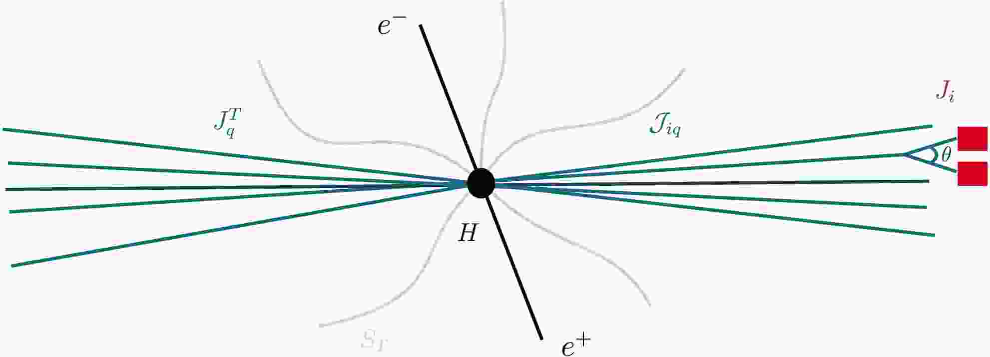
For phenomenological convenience, the observable is defined to be differential in the thrust variable τ and cumulative in the energy-correlation angle z. The thrust soft function $ S_T $ captures wide-angle soft emissions, while $ J^T_{\bar q} $ denotes the standard thrust jet function for the unmeasured opposite hemisphere. The perturbative matching coefficients $ {{\cal{J}}}_{iq} $ were derived at one-loop order in Ref. [43] and subsequently computed to two-loop accuracy in Ref. [49]. The physical processes defining Region 1 are illustrated in Fig. 1, and the corresponding factorized momentum modes are shown in the left panel of Fig. 2. All known factorized ingredients and their associated anomalous dimensions are summarized in Appendix A.1 up to the highest available perturbative accuracy.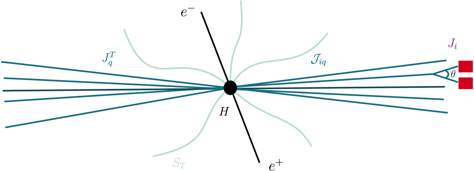

Figure 1.  (color online) A schematic of the configuration in Region 1. The black disc denotes the hard interaction H; the (cyan) jets are described by $ J^T_q $ and $ {\cal{J}}_{iq} $; the (green) soft radiation is contained in $ S_T $; and $ J_i $ denotes the collinear EEC jet function.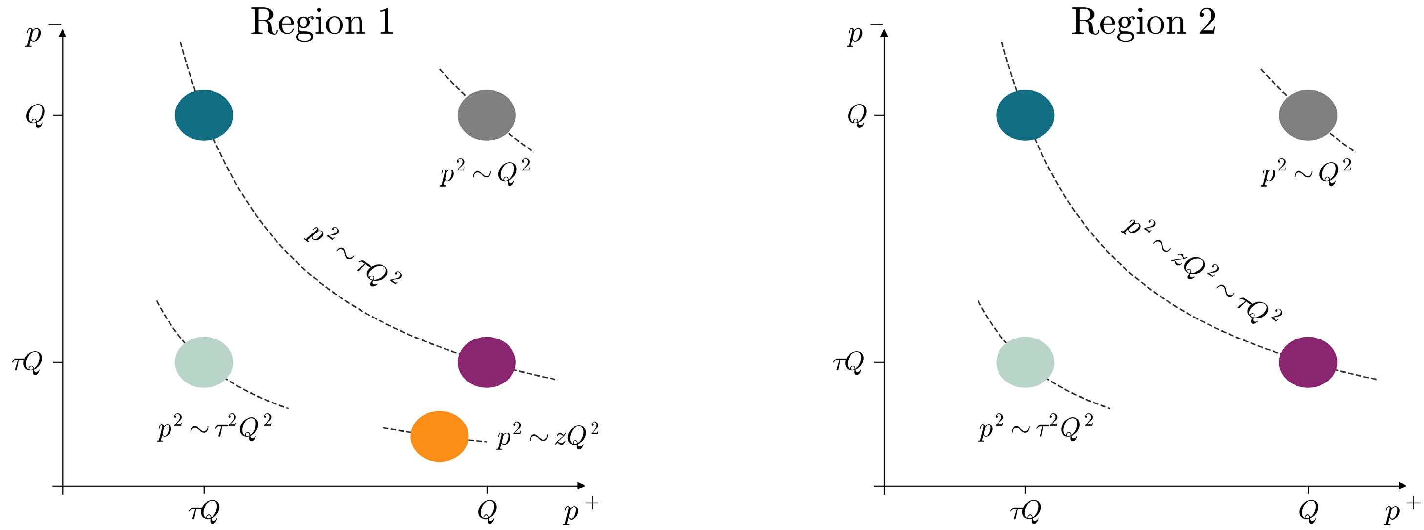

Figure 2.  (color online) Schematic representation of the factorized momentum-scaling modes governing the two collinear kinematic regimes. The hard (gray), collinear (cyan/purple), and soft (pale green) modes are shown. In Region 2, the two collinear sectors exhibit asymmetric scaling. By contrast, in Region 1, one of the collinear sectors undergoes further refactorization into additional submodes to properly resolve the $ \tau/z $ scale hierarchy.

Finally, although the RG evolution of the global thrust components ($ {\cal{H}} $, $ S_T $, $ J^T_q $) follows standard multiplicative forms, the collinear evolution of the EEC jet function $ \vec{J} $ is complicated by flavor mixing and the running of the strong coupling. These evolution equations can be solved using a standard iterative approach, as detailed in Ref. [31].

In this intermediate kinematic regime, the local angular separation probed by the energy correlator becomes comparable to the global thrust constraint. Consequently, the parametric hierarchy between the correlator scale and the thrust jet scale collapses ($ \mu_{{\rm{EEC}}} \sim \mu_J $). This collapse precludes the appearance of large logarithms of $ z/\tau $, thereby eliminating the need for the sub-jet refactorization used in Region 1. The factorization theorem therefore simplifies naturally, reducing to a form structurally analogous to the standard inclusive thrust distribution, given by

The novel ingredient in this regime is the collinear thrust-EEC jet function, $ J_{Tq} $, which describes collinear radiation constrained simultaneously by the global thrust variable τ and the local energy correlation z. The explicit one-loop calculation of $ J_{Tq} $ is presented in Appendix A.2 and demonstrates that its divergence structure exactly matches that of the standard thrust jet function.

By solving the standard RG equations and evolving all functions to the jet scale $ \mu_j $, the resummed cross section in Region 2 is given by

Here, the natural renormalization scales for the factorized components are determined by the physical kinematics as

Having examined the collinear limit within a single jet, we now turn to the back-to-back limit, $ z \to 1 $, in which the energy correlator probes correlations between particles in opposite hemispheres. While the inclusive EEC in this endpoint regime is governed entirely by standard TMD dynamics, imposing the global thrust constraint τ restricts the soft-radiation phase space and therefore necessitates a fundamental modification of the factorization structure.

This joint observable belongs to a class of multiscale configurations that entangle both $ {\rm{SCET}}_{{\rm{I}}} $ and $ {\rm{SCET}}_{{\rm{II}}} $ modes, requiring the $ {\rm{SCET}}_{+} $ formalism originally introduced in Ref. [25]. This framework has been successfully applied to the joint resummation of 0-jettiness and transverse momentum [26, 27], and more recently extended to thrust and transverse momentum [28]. Because the EEC in the $ z \to 1 $ limit effectively acts as a TMD measurement, the factorization structure for the joint $ (\tau, z) $ distribution emerges as a natural, albeit highly nontrivial, theoretical extension.

As illustrated previously in Fig. 3, the back-to-back regime subdivides into three distinct scaling regions, dictated by the dynamical interplay among the thrust jet scale $ \sqrt{\tau}Q $, the energy-correlation scale $ \sqrt{1-z}\, Q $, and the thrust soft scale $ \tau Q $. We begin our analysis with Region 3, defined by the scaling $ \sqrt{\tau} \gg \sqrt{1-z} \sim \tau $. This configuration corresponds to an $ {\rm{SCET}}_{{\rm{II}}} $ scenario in which the local energy-correlation scale is parametrically commensurate with the global thrust soft scale. The factorization theorem in this regime takes the form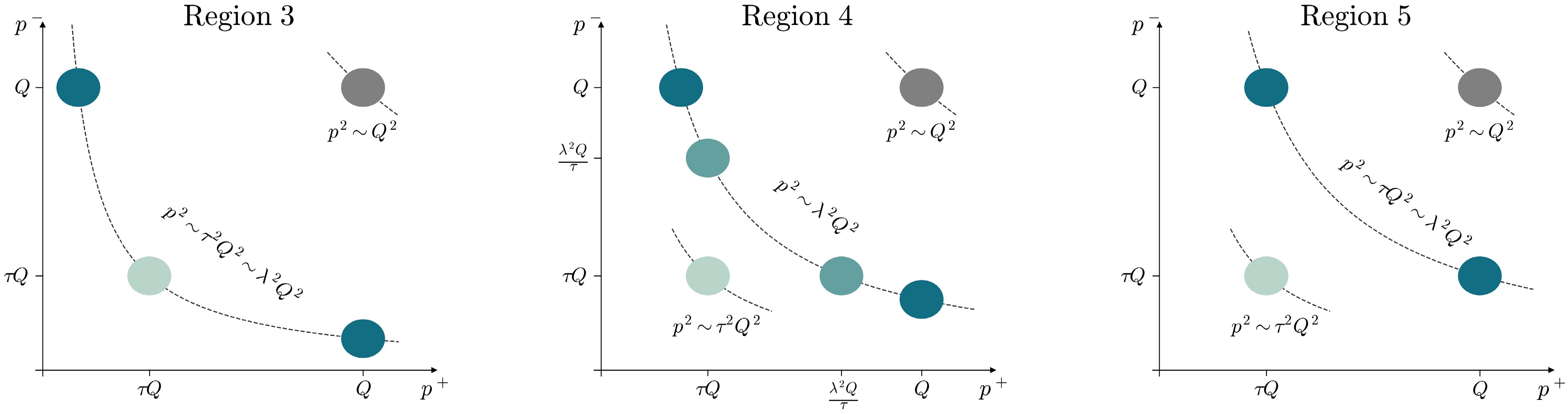

Figure 3.  (color online) The modes in the three regions are indicated as follows: hard (gray), collinear (cyan), soft (pea green), and collinear-soft (pale cyan). Regions 3–5 correspond to $ {\rm{SCET}}_{{\rm{II}}} $, $ {\rm{SCET}}_{{\rm{+}}} $, and $ {\rm{SCET}}_{{\rm{I}}} $, respectively.

Here, the thrust-TMD soft function, denoted by $ S_{pp} $, is a double-differential function that was originally derived and evaluated in momentum space in Ref. [26]. A cumulative momentum-space expression suitable for numerical implementation was subsequently provided in Ref. [27]. However, in Appendix A.3, we present a recalculation of $ S_{pp} $ directly in impact-parameter space using a four-dimensional scheme, yielding a remarkably compact analytic expression that significantly streamlines the resummation framework.

By solving the associated RG and rapidity renormalization group (RRG) equations and evolving all ingredients to the characteristic correlation scale $ \mu_b $, the resummed cross section becomes

where the natural renormalization and rapidity scales for the factorized components are given by

We note that, because the integration contour for the inverse transform in Eq. (12) inevitably extends into the nonperturbative regime, an appropriate regularization prescription must be employed to properly avoid the Landau pole.

As the kinematics transition further into this intermediate regime, the hierarchy between the local energy-correlation scale, $ Q\sqrt{1-z} $, and the global thrust soft scale, $ Q\tau $, becomes parametrically large. This pronounced scale separation invalidates the fixed-order treatment of the double-differential soft function $ S_{pp} $ used in Region 3. Consequently, a further refactorization of the underlying effective theory into an $ {\rm{SCET}}_{+} $ framework is required. Specifically, the soft dynamics decouple completely into the standard global thrust soft function, $ S_T $, and a pair of collinear-soft functions, $ {\cal{C}}_{q,\bar{q}} $, which describe soft fluctuations strictly localized near the respective jet boundaries. This structural refactorization is expressed as

This factorized separation facilitates the resummation of large logarithms of the conjugate ratio $ b_T^2Q^2/u^2 $, which corresponds to the physical parameter $ \tau^2/(1-z) $, through the coupled renormalization group evolution of the collinear-soft and thrust soft functions. Furthermore, because the EEC jet function and the collinear-soft function resolve the same invariant mass scale in this regime, their rapidity divergences must cancel exactly against one another, thereby ensuring the mathematical consistency of the joint factorization.

To systematically disentangle these overlapping dynamics, we introduce the power-counting parameter $ \lambda=q_T/Q \sim \sqrt{1-z} $. The six relevant momentum modes governing this $ {\rm{SCET}}_{+} $ hierarchy are then classified as follows

● hard: $\;\;\qquad\qquad p_h^\mu \sim Q(1,1,1), $

● $n\text{-}{\bf collinear}: \qquad p_c^\mu \sim Q(\lambda^2,1,\lambda), $

● $ \bar{n} $-collinear: $\qquad p_{\bar{c}}^\mu \sim Q(1,\lambda^2,\lambda), $

● n-collinear-soft: 　$ p_{cs}^\mu \sim Q(\tau,\lambda^2/\tau,\lambda), $

● $ \bar{n} $-collinear-soft:　 $ p_{\bar{c}s}^\mu \sim Q(\lambda^2/\tau,\tau,\lambda), $

● soft: $ \;\quad\quad\qquad\qquad p_s^\mu \sim Q(\tau,\tau,\tau). $

Applying this mode expansion, the factorization theorem in this regime takes the following form

By solving the associated evolution equations and evolving all functions to the characteristic energy correlation scale $ \mu_b $, the fully resummed cross section becomes

where the natural renormalization and rapidity scales associated with these distinct dynamics are evaluated as

Finally, we consider Region 5, in which the local energy-correlation scale explicitly matches the thrust collinear scale, $ \sqrt{1-z} \sim \sqrt{\tau} $. As this internal scale hierarchy collapses, the distinct collinear-soft modes recombine into standard collinear modes. The effective theory therefore reduces cleanly to a standard $ {\rm{SCET}}_{{\rm{I}}} $ framework. In this regime, all collinear dynamics are governed entirely by the back-to-back thrust-EEC jet function, $ {\cal{J}}_{Tq} $, which simultaneously resolves both the jet invariant mass and the internal energy correlations. The explicit one-loop calculation of this function is presented in Appendix A.4. Consequently, the factorization theorem simplifies to

By solving the standard RG equations to evolve the hard and soft functions to the common energy-correlation scale $ \mu_b $, we obtain the fully resummed cross section for Region 5 as

where the characteristic scales governing this configuration are defined as follows:

We conclude this section by detailing the matching procedure required to combine continuously the predictions obtained in the various kinematic regimes. Because the collinear and back-to-back limits are governed by distinct factorization theorems with different relevant scales, we first consider the back-to-back sector as an illustrative example.

In this sector, Region 4 exhibits the largest scale hierarchy and therefore resums the most complete set of large logarithms. However, the associated power corrections in Eq. (15) become unsuppressed as the physical boundaries of Regions 3 and 5 are approached. To account for this, we implement an additive matching scheme governed by profile scales. Although the practical numerical implementation of these profile functions is described in detail in Ref. [27], we outline the underlying methodology here. We begin with the standard matching of Region 4 onto fixed-order QCD.

Here, the subscript $ \mu_4 $ denotes evaluation at the natural scales defined in Section II.D, while $ \mu_{{\rm{FO}}} $ denotes the renormalization scale used in the fixed-order perturbative calculation for $ {\rm{d}}\Sigma_{{\rm{FO}}} $. Deep within Region 4, the fixed-order matching corrections are kinematically suppressed, and the matched cross section correctly reduces to the resummed result $ {\rm{d}}\Sigma_4/({\rm{d}}z{\rm{d}}\tau)|_{\mu_4} $. Conversely, as one approaches the fixed-order limit, the profile functions enforce the scale variation $ \mu_4 \to \mu_{{\rm{FO}}} $, thereby smoothly turning off the resummation. Through the explicit cancellation of the asymptotic terms within the parentheses, this additive formula simplifies exactly to the pure fixed-order cross section, $ {\rm{d}}\Sigma_{{\rm{FO}}}/({\rm{d}}z{\rm{d}}\tau)|_{\mu_{{\rm{FO}}}} $.

Generalizing this logic to capture the entire $ {\rm{SCET}}_{+} $ hierarchy, the fully matched expression encompassing all back-to-back regions is given by

This structure strictly enforces the correct asymptotic behavior in all limits. For example, when transitioning toward Region 3, the profile-scale convergence $ \mu_4 \to \mu_3 $ effectively deactivates the Region 4 resummation. The first two terms then merge to yield the expected Region 3 prediction $ {\rm{d}}\Sigma_3/({\rm{d}}z{\rm{d}}\tau)|_{\mu_3} $, while the remaining terms are naturally rendered as dynamically power-suppressed corrections. Furthermore, deep in the regime of validity of fixed-order perturbation theory, all resummation scales $ \mu_i $ uniformly merge to $ \mu_{{\rm{FO}}} $. This leads to an exact cancellation of the singular terms across all bracketed expressions, thereby cleanly recovering the full-theory fixed-order prediction.

An entirely analogous additive matching scheme is employed in the collinear sector to smoothly interpolate between Regions 1 and 2, and is given by

Ultimately, combining these piecewise-matched results guarantees a theoretically robust interpolation across the corresponding regions of the joint $ (\tau, z) $ phase space.

In this work, our primary focus is to establish the theoretical factorization framework for the joint thrust and EEC measurement. The numerical study in this section is intended as a qualitative phenomenological illustration of the kinematic effects induced by the thrust constraint. A complete numerical implementation of our resummation formula at high logarithmic accuracy requires careful treatment of multidimensional profile scales and shape functions, which we leave for future work. Nevertheless, to explore the physical effects of this multiscale hierarchy, we analyze the double-differential cross section generated by Pʏᴛʜɪᴀ 8.3 [50]. By incorporating coherent parton showers and hadronization models, Pʏᴛʜɪᴀ provides a reliable qualitative proxy for the complex QCD dynamics in these restricted phase-space regions.

The simulation is performed for $ e^+e^- \to \gamma^*/Z \to q\bar q $ at $ Q=91.2 $ GeV with five quark flavors. We generated $ 2\times 10^8 $ accepted events using the default Pʏᴛʜɪᴀ 8.3 shower and hadronization model. Both thrust and the EEC are evaluated using final-state charged particles. The two-dimensional distribution in Fig. 4 is globally normalized over the generated sample, and the one-dimensional curves in the right panel are globally normalized projections in the indicated thrust bins rather than distributions normalized separately within each bin.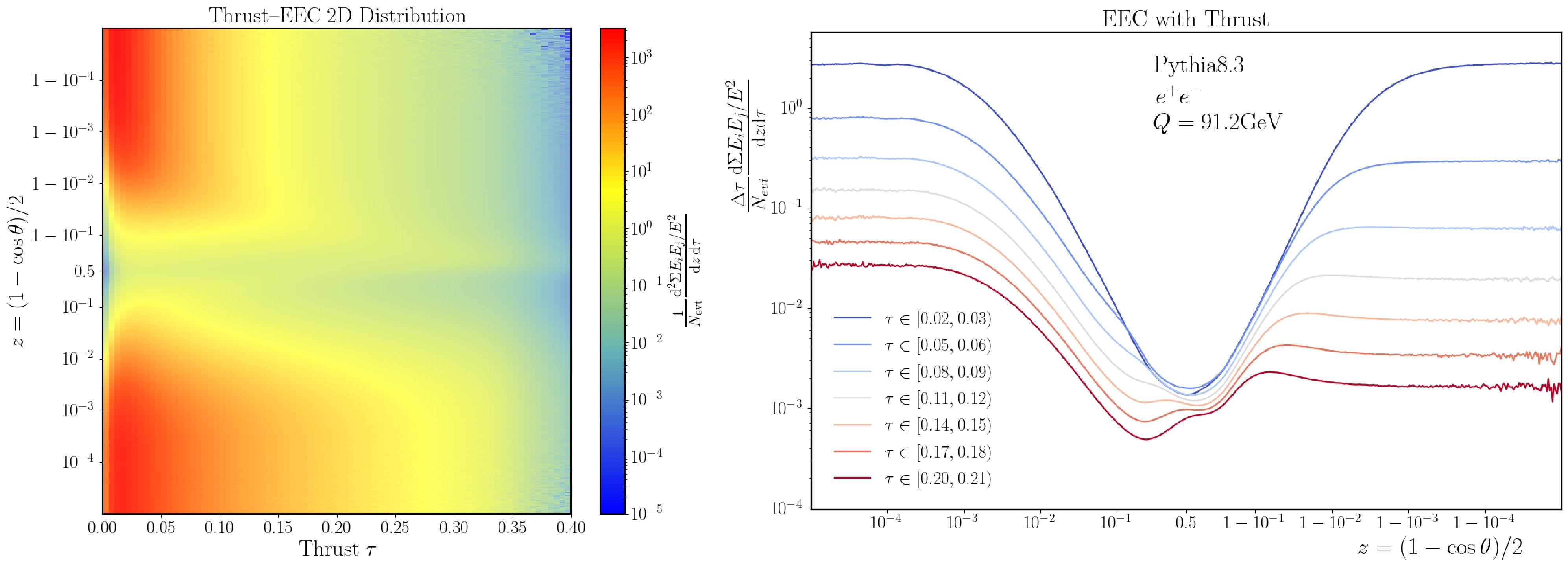

Figure 4.  (color online) Dependence of the EEC on the event shape for $ e^+e^- \to \gamma^*/Z \to q\bar q $ at $ Q=91.2 $ GeV, evaluated using final-state charged particles. The left panel shows the globally normalized two-dimensional distribution of the joint cross section as a function of τ and z. The right panel shows the globally normalized differential cross section as a function of $ {{\rm{cos}}}\theta $ for different thrust bins.

We first examine the inclusive kinematic distribution. As the two-dimensional spectrum in the left panel of Fig. 4 shows, most of the cross section naturally lies in highly collimated configurations (small τ) and at extreme angles.

To understand how the global event shape modifies the local correlations, we slice this distribution into narrow thrust bins ($ T = 1-\tau $), as shown in the right panel. Using the geometric mapping $ z = (1-{{\rm{cos}}}\theta)/2 $, the regions $ {{\rm{cos}}}\theta \to 1 $ and $ {{\rm{cos}}}\theta \to -1 $ map directly to the collinear ($ z \to 0 $) and back-to-back ($ z \to 1 $) limits.

The global thrust constraint strongly affects these extreme limits. For highly collimated events (small τ, large T), the tight phase-space restriction produces narrow plateaus in both regions. As τ increases (and T decreases), the relaxation of the phase-space boundary allows more wide-angle emissions. We observe that this kinematic interplay is highly asymmetric, with the back-to-back limit exhibiting much greater sensitivity to the thrust constraint than the collinear sector. Because of this asymmetric sensitivity, the back-to-back plateau broadens to span a much wider angular range. Concurrently, although the absolute heights of both plateaus decrease, the back-to-back plateau drops much more rapidly. Driven by this rapid asymmetric suppression, the distribution at larger τ values develops a distinct shoulder structure, visible as a protrusion just to the right of the distribution minimum.

These dynamical features explain why standard inclusive methods fail. An inclusive calculation cannot capture how a global thrust cut unevenly restricts soft and collinear radiation, nor can it predict the emergence of such local structures. Therefore, the joint resummation framework developed here is required to analytically describe this complex behavior.

In this paper, we established a joint factorization and resummation framework for the EEC and thrust in $ e^+e^- $ collisions. Working within the SCET formalism, we resolved the factorization structure at the collinear and back-to-back boundaries of the EEC. By analyzing the interplay between the local angle z and the global event shape τ, we identified five distinct kinematic regimes that cover the relevant limits. For each regime, we derived the corresponding factorization theorems and calculated the required perturbative components at one-loop order. Most importantly, we explicitly derived the joint collinear thrust-EEC jet function, $ J_{Tq} $, and the back-to-back thrust-EEC jet function, $ {\cal{J}}_{Tq} $.

We also explored the physical effects of this multiscale hierarchy using Pʏᴛʜɪᴀ 8.3 as a qualitative illustration. Our analysis revealed a highly asymmetric kinematic interplay. The back-to-back correlation is much more sensitive to the global thrust constraint than the collinear correlation. As a result of this asymmetric sensitivity, the back-to-back plateau broadens but its event rate decreases rapidly as τ increases. Standard inclusive methods cannot predict this uneven suppression of soft and collinear radiation. Therefore, our joint resummation framework provides the essential theoretical tool for properly describing these complex features.

Looking ahead, this work opens several avenues for future study. On the theory side, we plan to implement the full numerical resummation of the formulas derived here. To obtain high-precision theoretical predictions, future studies must also extend this joint resummation to higher logarithmic accuracy. This will require computing $ J_{Tq} $ and $ {\cal{J}}_{Tq} $ to two-loop order, together with a careful treatment of profile scales and nonperturbative parametrizations. On the experimental side, our framework provides a solid theoretical baseline for measurements at BESIII, Belle II, and the future Super-Tau Charm Factory, where global shape cuts are crucial for isolating specific jet configurations and suppressing backgrounds. At fixed-energy $ e^+e^- $ facilities, thrust binning can provide an internal scale scan for EEC measurements, offering complementary input for $ \alpha_s $ extractions. It also has the potential to be extended to polarized EECs to probe how spin correlations evolve under varying radiation patterns. Finally, the techniques developed here to connect local energy correlators with global event boundaries can be naturally extended to deep inelastic scattering at the future EIC or to joint measurements of the EEC and jet mass at the LHC.

For a compact representation of the factorization theorems, we adopt the following definitions of the Fourier and Laplace transforms and their respective inverses.

● $ \vec{H}=\{H_q,H_g\}^T $ denotes the inclusive hard functions for the quark and gluon sectors, known to three loops in the $ e^+e^- $ case [51] and to two loops for many processes at the LHC [52, 53].

● $ {\cal{H}}(Q,\mu) $ is the quark color-singlet SCET hard function, corresponding to the IR-finite part of the quark form factors [54−63], and can be derived from the recent result of Ref. [63] up to four loops.

● $ \vec{J}= \{J_q, J_g\} $ represents the collinear EEC jet functions, which are known to two-loop order from Ref. [31].

● $ {\cal{J}}_q\left(b_T, Q, \mu, \nu\right) $ denotes the TMD quark EEC jet function, which is known up to three-loop order [38].

● $ S(b_T, \mu, \nu) $ is the TMD soft function, known up to three loops, as reported in [64].

● The jet function $ J^{T}_{q}\left(u/{Q^2},\mu\right) $ and the soft function $ S_T\left(u/Q,\mu\right) $ for thrust (2-jettiness) are currently known to three-loop accuracy [65, 66]. Recent progress toward the four-loop level has been reported in [67].

● The two-loop matching coefficients $ {{\cal{J}}}_{ij} $ are given in [49].

● The one-loop double-differential thrust-TMD collinear-soft function is given in [26].

● The cusp anomalous dimension has been computed through four loops in [68−71], and an approximate five-loop expression was reported in [72].

● The five-loop beta function is given in [73, 74].

● The four-loop rapidity anomalous dimension is given in [40, 75].

● The three-loop timelike DGLAP anomalous dimensions are given in [76−78], and progress at four loops can be found in [68, 69, 79−90].

For the joint EEC-thrust observable, the resummation accuracy supported by the currently available ingredients is as follows. Region 1 can be systematically matched to $ {\rm{N}}^3{\rm{LL}} $ accuracy. Regions 2, 4, and 5 currently achieve $ {\rm{NNLL}} $ accuracy, since the newly introduced functions $ J_{Tq} $, $ {\cal{C}}_q $, and $ {\cal{J}}_{Tq} $ are computed to one loop in this work. Region 3 is similarly limited to $ {\rm{NNLL}} $ accuracy by the thrust-TMD soft function $ S_{pp} $, which is also evaluated at one loop here. Improving these results requires higher-order calculations of the corresponding boundary functions. Specifically, extending $ J_{Tq} $, $ {\cal{C}}_q $, $ {\cal{J}}_{Tq} $, and $ S_{pp} $ to two loops would promote Regions 2–5 to $ {\rm{N}}^3{\rm{LL}} $ accuracy.

In this subsection, we present the calculation of the bare one-loop collinear thrust-EEC jet function, $ J_{Tq}^{{\rm{bare}}} $. The relevant Feynman diagrams are shown in Fig. A1. The diagrams arising from the perturbative expansion of the Wilson lines vanish because we work in light-cone gauge. Notably, although diagrams (b) and (c) vanish as scaleless integrals in the standard inclusive EEC calculation, the additional constraint imposed by thrust introduces an explicit physical scale and therefore makes these integrals non-vanishing. Consequently, the complete bare one-loop result requires summing all three diagrams:

Figure A1.  (color online) Representative one-loop diagrams for the collinear thrust-EEC jet function, where the red dots denote insertions of the EEC operators.

where $ d=4-2\epsilon $, the index $ i \in \{q,g\} $ runs over the final-state partons after the splitting, and the sum over $ D \in \{(a),(b),(c)\} $ accounts for the three relevant diagrams. Here, y denotes the energy fraction carried by the quark, and $ s = k_T^2/(y(1-y)) $ is the invariant mass of the collinear pair. The diagram-specific EEC measurement weights are given by

To parameterize the kinematics, we introduce two light-like reference vectors, $ n^\mu = (1,0,0,1) $ and $ \bar{n}^\mu = (1,0,0,-1) $, in Minkowski space, such that any four-momentum can be decomposed as $ k^\mu = \left( n\cdot k, \bar{n} \cdot k , k^\mu_\perp \right)= (k^+, k^-, k^\mu_\perp) $. For quark-initiated splittings, the relevant bare splitting kernels are

For diagrams (b) and (c), the evaluation is straightforward and yields

where $ L_u \equiv {{\rm{ln}}}\left(ue^{\gamma_E}\mu^2/Q^2\right) $. Evaluating diagram (a) requires the explicit insertion of the phase-space constraint $ \Theta(z - s/k^-p^-) $ and a symmetry factor of 2, as in Eq. (A3). This yields

where $ L_{z}={\rm{ln}}(zQ^2/\mu^2) $. The finite term $ j^q(u,z) $ contains nontrivial kinematic dependence

where $ {\rm{erfi}}(x) $ denotes the imaginary error function. Summing the contributions from all three diagrams, we obtain the bare one-loop collinear thrust-EEC jet function as

Crucially, the divergent terms in this result exactly match those of the standard inclusive thrust jet function, ensuring that the RG consistency condition is satisfied. We perform renormalization in the $ \overline{{\rm{MS}}} $ scheme, which is used throughout the remainder of this work. The renormalized jet function $ J_{Tq} $ is related to the bare function by $ J_{Tq} = Z_{J} J_{Tq}^{{\rm{bare}}} $, where the renormalization constant $ Z_J $ absorbs the $ 1/\epsilon $ poles. The renormalized collinear thrust-EEC jet function therefore obeys the evolution equation:

where $ \gamma_J(\alpha_s) $ denotes the non-cusp anomalous dimension, which is given in Ref. [67] up to four-loop order. Physically, diagrams (b) and (c) represent self-correlations in which both detectors probe the same parton. At strictly zero relative angle, their combined contributions are naturally independent of z. Furthermore, in the limit $ uz \to 0 $ in Region 1, diagram (a) alone reproduces the collinear quark EEC jet function in Eq. (5).

In this subsection, we detail the calculation of the bare one-loop thrust-TMD soft function, $ S_{pp}^{{\rm{bare}}} $. Because a soft gluon can be emitted into either of the two thrust hemispheres, the complete one-loop soft integral is twice the single-hemisphere contribution.

Here, the step function $ \Theta(k^- - k^+) $ restricts the phase space to a single hemisphere, wherein the smaller light-cone component $ k^+ $ determines the contribution to the thrust observable.

Following Ref. [28], this one-loop result can be conveniently decomposed into the standard TMD soft function, $ S^{(1),{\rm{bare}}}_{{\rm{TMD}}} $, and a remainder term, $ \Delta S^{(1)} $, which represents the finite correction induced by the thrust constraint.

The standard bare TMD soft function is given by

where $L_b = 2{{\rm{ln}}} ({\rm e}^{\gamma_E} b_T \mu /2)$. Since all ultraviolet and rapidity divergences are fully captured by the standard TMD soft function, the remaining correction $ \Delta S^{(1)} $ is manifestly finite. We can explicitly isolate this finite contribution by partitioning the phase-space integrand using the following algebraic identity

Integration of the first term reproduces the standard TMD soft function. Evaluating the second term directly in four dimensions yields the following compact analytic result:

where we have defined the dimensionless scaling variable $ c \equiv b_T Q/u $. Finally, the renormalized thrust-TMD soft function satisfies the corresponding RG and RRG equations as

where $ \gamma_S(\alpha_s) $ denotes the soft non-cusp anomalous dimension given in Ref. [64] up to three-loop order, and the four-loop rapidity anomalous dimension $ \gamma_\nu(\alpha_s) $ is provided in Refs. [40, 75].

In this subsection, we present the calculation of the one-loop bare TMD thrust-EEC jet function, $ {\cal{J}}_{Tq}^{{\rm{bare}}} $. The one-loop integral is given by

where

Crucially, because the divergence structure of this integral exactly matches that of the standard inclusive thrust jet function, we can employ the same subtraction scheme used in the previous section (Appendix A.3). By subtracting the standard thrust jet function at the integrand level, the remaining finite term can be evaluated directly in four dimensions. This procedure yields the complete one-loop expression:

where $ a \equiv b_T^2 Q^2 / (4u) $. The nontrivial kinematic dependence is encoded in the finite function $ j_0(a) $, which is given by

where $ G_{p, q}^{m, n} $ denotes the Meijer G-function. Notably, the one-loop TMD thrust-EEC jet function is identical to the standard thrust jet function, up to a shift by the finite term $ j_0(a) $. Furthermore, in the asymptotic limit $ a \to \infty $ (which corresponds to the pronounced scale hierarchy of Region 4), this double-differential jet function refactorizes exactly. At one loop, this appears additively as the sum of the standard EEC jet function and the thrust-TMD collinear-soft function,

The collinear-soft function $ {\cal{C}}_q $ that emerges in this limit is identical to the one that decouples from the double-differential soft function in Eq. (14). This confirms the universality of the collinear-soft mode and demonstrates the consistency of our factorization framework. The renormalized TMD thrust-EEC jet function satisfies the corresponding RG equations as