


 Abstract
 HTML
 Reference
 Related
 PDF




-
Exotic Higgs decays to long-lived scalars,
$ h\to ss $ with$ s\to b\bar b $ , are among the most well-motivated signatures of a hidden sector coupled to the SM through the Higgs portal [1–7]. Dedicated searches at the LHC reconstruct the displaced secondary vertex (SV) produced by the scalar decay from its spatial displacement alone [8, 9]. Recent ATLAS and CMS analyses have pushed these purely spatial searches to high sensitivity: the ATLAS Run-2 displaced-vertex search [10] targets hadronic long-lived particles (LLPs) in the mass range$ m_s\simeq5\text{–}55 \,{\rm{GeV}} $ , includes a VBF-tagged signal region, and sets the strongest current limits for$ c\tau\lesssim100 \,{\rm{mm}} $ ; the CMS Run-3 light-LLP displaced-jets search [11] achieves up to an order-of-magnitude improvement over earlier results for$ m_s\lesssim60 \,{\rm{GeV}} $ and$ c\tau\lesssim1\,{\rm{m}} $ through dedicated triggers, improved reconstruction, and machine-learning discriminants [12, 13]. In their most sensitive displacement-limited regions, however, these analyses are already constrained by the systematic uncertainty of the data-driven background estimate rather than by the available luminosity: additional spatial information or luminosity alone cannot break this ceiling. Displacement provides only half of the kinematic information carried by a long-lived decay: a particle that travels a macroscopic distance before decaying also produces tracks that arrive late, and this delay grows with the same flight distance that the spatial search exploits.Precision timing turns that delay into an independent observable. The arrival time of long-lived decay products has been proposed as a means to reconstruct LLP kinematics and lifetimes [14–16], to trigger on displaced jets [17], and, in the pioneering study of Ref. [18], to suppress the prompt background to a neutral long-lived particle by an order of magnitude using a
$ {\cal{O}}(30 \,{\rm{ps}}) $ timing layer at the HL-LHC [19]. That study used an initial-state-radiation jet as the timing reference, leaving open the question of how to obtain a clean, reproducible start time$ t_0 $ in the realistic high-pileup environment of the HL-LHC, where an ISR jet is neither guaranteed nor unambiguously prompt. The present work is not the first to propose timing for long-lived particles; its novelty lies in identifying a specific configuration in which the event start time is provided by the same objects that define the signal region, making it available event by event and tying it unambiguously to the hard scatter.Vector-boson fusion provides exactly this configuration. The two forward, high-mass tag jets that strengthen the spatial selection also tag the hard-scatter vertex with high purity; VBF has previously been used as a production and trigger handle for long-lived particles [20], but here it plays a new role as the enabler of the timing reference. The CMS Phase-2 upgrade adds a MIP Timing Detector (MTD) [21], whose Barrel Timing Layer (BTL,
$ |\eta|<1.48 $ ) timestamps charged tracks with a resolution of$ \simeq30\text{–}60 \,{\rm{ps}} $ ; its detailed parameters are given below. Such a CMS-MTD-like barrel layer times the prompt central tracks of the VBF-tagged vertex to determine$ t_0 $ , and the same layer times the central tracks of the displaced vertex under study. The VBF requirement that defines the signal region is therefore identical to the requirement that provides the temporal reference. The VBF jets themselves supply no timing measurement; the reference is instead the production time of the prompt central tracks of the vertex they tag. A realistic HL-LHC analysis would combine several complementary handles—prompt-track timing, primary-vertex time, calorimeter or jet timing, and object-to-vertex association [22]—of which we deliberately isolate the single cleanest one here.In this Letter we present, to our knowledge, the first study to use the VBF-tagged hard-scatter vertex as the event-by-event timing reference for four-dimensional (4D) displaced-vertex reconstruction of long-lived scalars at the HL-LHC. Our aim is not to reproduce the full experimental searches, whose background estimates are necessarily data driven, but to isolate the incremental information carried by vertex time once a spatial displaced-vertex candidate has been reconstructed. Because a fast detector simulation cannot determine the absolute background normalization, we quote a normalization-free figure of merit—the gain in
$ S/\sqrt{B} $ from adding timing to an otherwise identical spatial selection—and map it across the scalar mass–lifetime plane. To place this gain in physical context, we also translate the selection into illustrative, statistics-limited 95% confidence-level (CL) limits on the branching ratio$ {\rm{BR}}(h\to ss) $ —under the explicit assumption$ {\rm{BR}}(s\to b\bar b)=1 $ , equivalently a limit on the product$ {\rm{BR}}(h\to ss)\,[{\rm{BR}}(s\to b\bar b)]^2 $ for this topology—using the standard asymptotic modified-frequentist ($ {\rm{CL}}_s $ ) procedure. The central result is a structural one: the timing gain reverses its dependence on scalar mass at a decay length of$ c\tau\simeq100 \,{\rm{mm}} $ , the point at which boost-driven and containment-driven effects balance, and it grows with lifetime precisely where purely spatial searches lose tracker acceptance. -
Exotic Higgs decays to long-lived scalars,
$ h\to ss $ with$ s\to b\bar b $ , are among the most well-motivated signatures of a hidden sector coupled to the SM through the Higgs portal [1–7]. Dedicated searches at the LHC reconstruct the displaced secondary vertex (SV) produced by the scalar decay from its spatial displacement alone [8, 9]. Recent ATLAS and CMS analyses have pushed these purely spatial searches to high sensitivity: the ATLAS Run-2 displaced-vertex search [10] targets hadronic long-lived particles (LLPs) in the mass range$ m_s\simeq5\text{–}55 \,{\rm{GeV}} $ , includes a VBF-tagged signal region, and sets the strongest current limits for$ c\tau\lesssim100 \,{\rm{mm}} $ ; the CMS Run-3 light-LLP displaced-jets search [11] achieves up to an order-of-magnitude improvement over earlier results for$ m_s\lesssim60 \,{\rm{GeV}} $ and$ c\tau\lesssim1\,{\rm{m}} $ through dedicated triggers, improved reconstruction, and machine-learning discriminants [12, 13]. In their most sensitive displacement-limited regions, however, these analyses are already constrained by the systematic uncertainty of the data-driven background estimate rather than by the available luminosity: additional spatial information or luminosity alone cannot break this ceiling. Displacement provides only half of the kinematic information carried by a long-lived decay: a particle that travels a macroscopic distance before decaying also produces tracks that arrive late, and this delay grows with the same flight distance that the spatial search exploits.Precision timing turns that delay into an independent observable. The arrival time of long-lived decay products has been proposed as a means to reconstruct LLP kinematics and lifetimes [14–16], to trigger on displaced jets [17], and, in the pioneering study of Ref. [18], to suppress the prompt background to a neutral long-lived particle by an order of magnitude using a
$ {\cal{O}}(30 \,{\rm{ps}}) $ timing layer at the HL-LHC [19]. That study used an initial-state-radiation jet as the timing reference, leaving open the question of how to obtain a clean, reproducible start time$ t_0 $ in the realistic high-pileup environment of the HL-LHC, where an ISR jet is neither guaranteed nor unambiguously prompt. The present work is not the first to propose timing for long-lived particles; its novelty lies in identifying a specific configuration in which the event start time is provided by the same objects that define the signal region, making it available event by event and tying it unambiguously to the hard scatter.Vector-boson fusion provides exactly this configuration. The two forward, high-mass tag jets that strengthen the spatial selection also tag the hard-scatter vertex with high purity; VBF has previously been used as a production and trigger handle for long-lived particles [20], but here it plays a new role as the enabler of the timing reference. The CMS Phase-2 upgrade adds a MIP Timing Detector (MTD) [21], whose Barrel Timing Layer (BTL,
$ |\eta|<1.48 $ ) timestamps charged tracks with a resolution of$ \simeq30\text{–}60 \,{\rm{ps}} $ ; its detailed parameters are given below. Such a CMS-MTD-like barrel layer times the prompt central tracks of the VBF-tagged vertex to determine$ t_0 $ , and the same layer times the central tracks of the displaced vertex under study. The VBF requirement that defines the signal region is therefore identical to the requirement that provides the temporal reference. The VBF jets themselves supply no timing measurement; the reference is instead the production time of the prompt central tracks of the vertex they tag. A realistic HL-LHC analysis would combine several complementary handles—prompt-track timing, primary-vertex time, calorimeter or jet timing, and object-to-vertex association [22]—of which we deliberately isolate the single cleanest one here.In this Letter we present, to our knowledge, the first study to use the VBF-tagged hard-scatter vertex as the event-by-event timing reference for four-dimensional (4D) displaced-vertex reconstruction of long-lived scalars at the HL-LHC. Our aim is not to reproduce the full experimental searches, whose background estimates are necessarily data driven, but to isolate the incremental information carried by vertex time once a spatial displaced-vertex candidate has been reconstructed. Because a fast detector simulation cannot determine the absolute background normalization, we quote a normalization-free figure of merit—the gain in
$ S/\sqrt{B} $ from adding timing to an otherwise identical spatial selection—and map it across the scalar mass–lifetime plane. To place this gain in physical context, we also translate the selection into illustrative, statistics-limited 95% confidence-level (CL) limits on the branching ratio$ {\rm{BR}}(h\to ss) $ —under the explicit assumption$ {\rm{BR}}(s\to b\bar b)=1 $ , equivalently a limit on the product$ {\rm{BR}}(h\to ss)\,[{\rm{BR}}(s\to b\bar b)]^2 $ for this topology—using the standard asymptotic modified-frequentist ($ {\rm{CL}}_s $ ) procedure. The central result is a structural one: the timing gain reverses its dependence on scalar mass at a decay length of$ c\tau\simeq100 \,{\rm{mm}} $ , the point at which boost-driven and containment-driven effects balance, and it grows with lifetime precisely where purely spatial searches lose tracker acceptance. -
Exotic Higgs decays to long-lived scalars,
$ h\to ss $ with$ s\to b\bar b $ , are among the most well-motivated signatures of a hidden sector coupled to the SM through the Higgs portal [1–7]. Dedicated searches at the LHC reconstruct the displaced secondary vertex (SV) produced by the scalar decay from its spatial displacement alone [8, 9]. Recent ATLAS and CMS analyses have pushed these purely spatial searches to high sensitivity: the ATLAS Run-2 displaced-vertex search [10] targets hadronic long-lived particles (LLPs) in the mass range$ m_s\simeq5\text{–}55 \,{\rm{GeV}} $ , includes a VBF-tagged signal region, and sets the strongest current limits for$ c\tau\lesssim100 \,{\rm{mm}} $ ; the CMS Run-3 light-LLP displaced-jets search [11] achieves up to an order-of-magnitude improvement over earlier results for$ m_s\lesssim60 \,{\rm{GeV}} $ and$ c\tau\lesssim1\,{\rm{m}} $ through dedicated triggers, improved reconstruction, and machine-learning discriminants [12, 13]. In their most sensitive displacement-limited regions, however, these analyses are already constrained by the systematic uncertainty of the data-driven background estimate rather than by the available luminosity: additional spatial information or luminosity alone cannot break this ceiling. Displacement provides only half of the kinematic information carried by a long-lived decay: a particle that travels a macroscopic distance before decaying also produces tracks that arrive late, and this delay grows with the same flight distance that the spatial search exploits.Precision timing turns that delay into an independent observable. The arrival time of long-lived decay products has been proposed as a means to reconstruct LLP kinematics and lifetimes [14–16], to trigger on displaced jets [17], and, in the pioneering study of Ref. [18], to suppress the prompt background to a neutral long-lived particle by an order of magnitude using a
$ {\cal{O}}(30 \,{\rm{ps}}) $ timing layer at the HL-LHC [19]. That study used an initial-state-radiation jet as the timing reference, leaving open the question of how to obtain a clean, reproducible start time$ t_0 $ in the realistic high-pileup environment of the HL-LHC, where an ISR jet is neither guaranteed nor unambiguously prompt. The present work is not the first to propose timing for long-lived particles; its novelty lies in identifying a specific configuration in which the event start time is provided by the same objects that define the signal region, making it available event by event and tying it unambiguously to the hard scatter.Vector-boson fusion provides exactly this configuration. The two forward, high-mass tag jets that strengthen the spatial selection also tag the hard-scatter vertex with high purity; VBF has previously been used as a production and trigger handle for long-lived particles [20], but here it plays a new role as the enabler of the timing reference. The CMS Phase-2 upgrade adds a MIP Timing Detector (MTD) [21], whose Barrel Timing Layer (BTL,
$ |\eta|<1.48 $ ) timestamps charged tracks with a resolution of$ \simeq30\text{–}60 \,{\rm{ps}} $ ; its detailed parameters are given below. Such a CMS-MTD-like barrel layer times the prompt central tracks of the VBF-tagged vertex to determine$ t_0 $ , and the same layer times the central tracks of the displaced vertex under study. The VBF requirement that defines the signal region is therefore identical to the requirement that provides the temporal reference. The VBF jets themselves supply no timing measurement; the reference is instead the production time of the prompt central tracks of the vertex they tag. A realistic HL-LHC analysis would combine several complementary handles—prompt-track timing, primary-vertex time, calorimeter or jet timing, and object-to-vertex association [22]—of which we deliberately isolate the single cleanest one here.In this Letter we present, to our knowledge, the first study to use the VBF-tagged hard-scatter vertex as the event-by-event timing reference for four-dimensional (4D) displaced-vertex reconstruction of long-lived scalars at the HL-LHC. Our aim is not to reproduce the full experimental searches, whose background estimates are necessarily data driven, but to isolate the incremental information carried by vertex time once a spatial displaced-vertex candidate has been reconstructed. Because a fast detector simulation cannot determine the absolute background normalization, we quote a normalization-free figure of merit—the gain in
$ S/\sqrt{B} $ from adding timing to an otherwise identical spatial selection—and map it across the scalar mass–lifetime plane. To place this gain in physical context, we also translate the selection into illustrative, statistics-limited 95% confidence-level (CL) limits on the branching ratio$ {\rm{BR}}(h\to ss) $ —under the explicit assumption$ {\rm{BR}}(s\to b\bar b)=1 $ , equivalently a limit on the product$ {\rm{BR}}(h\to ss)\,[{\rm{BR}}(s\to b\bar b)]^2 $ for this topology—using the standard asymptotic modified-frequentist ($ {\rm{CL}}_s $ ) procedure. The central result is a structural one: the timing gain reverses its dependence on scalar mass at a decay length of$ c\tau\simeq100 \,{\rm{mm}} $ , the point at which boost-driven and containment-driven effects balance, and it grows with lifetime precisely where purely spatial searches lose tracker acceptance. -
We study VBF Higgs production at the
$ 14 \,{\rm{TeV}} $ HL-LHC,$ pp\to hjj $ , followed by the prompt exotic decay$ h\to ss $ and the displaced decay$ s\to b\bar b $ of the long-lived scalar s, which travels a macroscopic distance before decaying. Each event contains two forward, high-mass tag jets recoiling against a Higgs boson whose decay yields one or two displaced$ b\bar b $ vertices. The tag jets originate from the hard-scatter vertex and identify it with high purity; the prompt central tracks of that vertex, timed by the barrel layer [21], determine$ t_0 $ , while the same barrel layer times the central tracks of the displaced vertex. The more forward coverage of an endcap timing detector [23] is not required, because the displaced$ b\bar b $ tracks recoiling against the forward tag jets are themselves central.Events are generated with MADGRAPH5_AMC@NLO [24] using the PDF4LHC21 set [25], showered and hadronized in
$\text{PYTHIA}$ 8.3 [26], and passed through a$\text{DELPHES}$ 3 [27] HL-LHC parametrization with a CMS-MTD-like barrel timing layer [28] ($ |\eta|<1.48 $ ,$ \sigma_t=30 \;{\rm{ps}} $ ,$ p_T>0.7 \,{\rm{GeV}} $ ) and pileup at$ \langle\mu\rangle=200 $ , consistent with the Phase-2 tracker environment [29]. Jets are clustered with the anti-$ k_T $ algorithm [30] ($ R=0.4 $ ) in FASTJET [31]. We scan$ c\tau\in\{1,10,30,100,300,1000\} \;{\rm{mm}} $ and$ m_s\in \{20,40,55,60\} \;{\rm{GeV}} $ , with the upper end approaching the$ m_s\to m_h/2 $ threshold. The signal and SM-Higgs samples are generated independently from the same run card; both carry the same generated cross section after the parton-level VBF acceptance,$ \sigma_{{\rm{gen}}}=0.1725 \;{\rm{pb}} $ , corresponding to$ N_{{\rm{gen}}}\simeq5.2\times10^{5} $ at$ {\cal{L}}=3000 \;{\rm{fb}}^{-1} $ . The signal and the electroweak and SM-Higgs backgrounds comprise$ 2\times10^{5} $ generated events each; the dominant QCD background is generated with$ 2.2\times10^{6} $ events to control the statistics of the late-time tail. For the gain figure of merit, all production normalizations cancel exactly. For the illustrative branching-fraction projection, we normalize the VBF Higgs yield to the LHC Higgs Cross Section Working Group$ 14 \;{\rm{TeV}} $ recommendation [32] and use the generator-level VBF filter only to evaluate the acceptance, while the QCD$ b\bar bjj $ continuum is treated as a nuisance parameter$ \kappa_b $ rather than as a prediction of the leading-order simulation (see below). -
We study VBF Higgs production at the
$ 14 \,{\rm{TeV}} $ HL-LHC,$ pp\to hjj $ , followed by the prompt exotic decay$ h\to ss $ and the displaced decay$ s\to b\bar b $ of the long-lived scalar s, which travels a macroscopic distance before decaying. Each event contains two forward, high-mass tag jets recoiling against a Higgs boson whose decay yields one or two displaced$ b\bar b $ vertices. The tag jets originate from the hard-scatter vertex and identify it with high purity; the prompt central tracks of that vertex, timed by the barrel layer [21], determine$ t_0 $ , while the same barrel layer times the central tracks of the displaced vertex. The more forward coverage of an endcap timing detector [23] is not required, because the displaced$ b\bar b $ tracks recoiling against the forward tag jets are themselves central.Events are generated with MADGRAPH5_AMC@NLO [24] using the PDF4LHC21 set [25], showered and hadronized in
$\text{PYTHIA}$ 8.3 [26], and passed through a$\text{DELPHES}$ 3 [27] HL-LHC parametrization with a CMS-MTD-like barrel timing layer [28] ($ |\eta|<1.48 $ ,$ \sigma_t=30 \;{\rm{ps}} $ ,$ p_T>0.7 \,{\rm{GeV}} $ ) and pileup at$ \langle\mu\rangle=200 $ , consistent with the Phase-2 tracker environment [29]. Jets are clustered with the anti-$ k_T $ algorithm [30] ($ R=0.4 $ ) in FASTJET [31]. We scan$ c\tau\in\{1,10,30,100,300,1000\} \;{\rm{mm}} $ and$ m_s\in \{20,40,55,60\} \;{\rm{GeV}} $ , with the upper end approaching the$ m_s\to m_h/2 $ threshold. The signal and SM-Higgs samples are generated independently from the same run card; both carry the same generated cross section after the parton-level VBF acceptance,$ \sigma_{{\rm{gen}}}=0.1725 \;{\rm{pb}} $ , corresponding to$ N_{{\rm{gen}}}\simeq5.2\times10^{5} $ at$ {\cal{L}}=3000 \;{\rm{fb}}^{-1} $ . The signal and the electroweak and SM-Higgs backgrounds comprise$ 2\times10^{5} $ generated events each; the dominant QCD background is generated with$ 2.2\times10^{6} $ events to control the statistics of the late-time tail. For the gain figure of merit, all production normalizations cancel exactly. For the illustrative branching-fraction projection, we normalize the VBF Higgs yield to the LHC Higgs Cross Section Working Group$ 14 \;{\rm{TeV}} $ recommendation [32] and use the generator-level VBF filter only to evaluate the acceptance, while the QCD$ b\bar bjj $ continuum is treated as a nuisance parameter$ \kappa_b $ rather than as a prediction of the leading-order simulation (see below). -
We study VBF Higgs production at the
$ 14 \,{\rm{TeV}} $ HL-LHC,$ pp\to hjj $ , followed by the prompt exotic decay$ h\to ss $ and the displaced decay$ s\to b\bar b $ of the long-lived scalar s, which travels a macroscopic distance before decaying. Each event contains two forward, high-mass tag jets recoiling against a Higgs boson whose decay yields one or two displaced$ b\bar b $ vertices. The tag jets originate from the hard-scatter vertex and identify it with high purity; the prompt central tracks of that vertex, timed by the barrel layer [21], determine$ t_0 $ , while the same barrel layer times the central tracks of the displaced vertex. The more forward coverage of an endcap timing detector [23] is not required, because the displaced$ b\bar b $ tracks recoiling against the forward tag jets are themselves central.Events are generated with MADGRAPH5_AMC@NLO [24] using the PDF4LHC21 set [25], showered and hadronized in
$\text{PYTHIA}$ 8.3 [26], and passed through a$\text{DELPHES}$ 3 [27] HL-LHC parametrization with a CMS-MTD-like barrel timing layer [28] ($ |\eta|<1.48 $ ,$ \sigma_t=30 \;{\rm{ps}} $ ,$ p_T>0.7 \,{\rm{GeV}} $ ) and pileup at$ \langle\mu\rangle=200 $ , consistent with the Phase-2 tracker environment [29]. Jets are clustered with the anti-$ k_T $ algorithm [30] ($ R=0.4 $ ) in FASTJET [31]. We scan$ c\tau\in\{1,10,30,100,300,1000\} \;{\rm{mm}} $ and$ m_s\in \{20,40,55,60\} \;{\rm{GeV}} $ , with the upper end approaching the$ m_s\to m_h/2 $ threshold. The signal and SM-Higgs samples are generated independently from the same run card; both carry the same generated cross section after the parton-level VBF acceptance,$ \sigma_{{\rm{gen}}}=0.1725 \;{\rm{pb}} $ , corresponding to$ N_{{\rm{gen}}}\simeq5.2\times10^{5} $ at$ {\cal{L}}=3000 \;{\rm{fb}}^{-1} $ . The signal and the electroweak and SM-Higgs backgrounds comprise$ 2\times10^{5} $ generated events each; the dominant QCD background is generated with$ 2.2\times10^{6} $ events to control the statistics of the late-time tail. For the gain figure of merit, all production normalizations cancel exactly. For the illustrative branching-fraction projection, we normalize the VBF Higgs yield to the LHC Higgs Cross Section Working Group$ 14 \;{\rm{TeV}} $ recommendation [32] and use the generator-level VBF filter only to evaluate the acceptance, while the QCD$ b\bar bjj $ continuum is treated as a nuisance parameter$ \kappa_b $ rather than as a prediction of the leading-order simulation (see below). -
We require at least two jets with
$ p_T^{j_1}>100 \;{\rm{GeV}} $ and$ p_T^{j_2}>80 \;{\rm{GeV}} $ , invariant mass$ m_{jj}>1200 \;{\rm{GeV}} $ , and a rapidity gap$ |\Delta\eta_{jj}|>4.0 $ . These cuts select the forward dijet configuration characteristic of VBF and suppress the gluon-initiated QCD continuum, whose central, lower-mass dijets rarely satisfy such a large gap; they accept 27.0% of generated signal at$ m_s=55 \;{\rm{GeV}} $ and a comparable fraction of the SM-Higgs background, as expected for two processes sharing VBF production kinematics. These requirements are chosen to be compatible with HL-LHC VBF-trigger strategies [17, 20, 33–35] and are independent of the displaced decay products, so the timing information is used offline in this baseline study. The offline thresholds sit well above those of a Phase-2 L1 VBF di-jet seed [34] (two jets with$ p_T\gtrsim40 \;{\rm{GeV}} $ and$ m_{jj}\gtrsim620 \;{\rm{GeV}} $ ): emulating such a seed retains$ \gtrsim $ 99.9% of the offline-selected signal, placing it on the trigger plateau, while a displaced-jet trigger [17] offers a complementary path.Displaced-vertex candidates are built from reconstructed tracks assigned to the hard-scatter vertex with
$ p_T>1 \;{\rm{GeV}} $ and transverse impact parameter$ |d_0|> 0.1 \,{\rm{mm}} $ , clustered by the proximity of their reconstructed points of closest approach with a single-linkage algorithm in three dimensions (linking distance$ 2 \,{\rm{mm}} $ ). Every cluster of at least three tracks whose reconstructed transverse radius$ R_{{\rm{SV}}} $ —the transverse distance of the vertex from the beam line—exceeds$ 3 \,{\rm{mm}} $ is a vertex candidate, and the highest-invariant-mass candidate among those passing the displacement requirement is taken as the displaced vertex of the event. Because$ h\to ss $ yields two long-lived scalars, an event is retained if at least one s decays inside the tracker and forms such a vertex; a second candidate, when present, is not used, which keeps the selection inclusive and defines the efficiency per event rather than per scalar. Requiring two displaced vertices would suppress the background further but would forfeit acceptance at long lifetime, where one scalar frequently escapes the tracker. This displacement-first choice is essential under pileup: selecting the highest-mass cluster overall instead picks a prompt, high-multiplicity pileup combination that then fails the displacement cut, simultaneously decimating the signal and driving the surviving background artificially to zero. We then require$ \displaystyle\sum p_T>10 \,{\rm{GeV}} $ for the vertex tracks and a mass-to-spread ratio$ m_{{\rm{SV}}}/\Delta R_{{\rm{max}}}>4 \,{\rm{GeV}} $ . The$ R_{{\rm{SV}}} $ requirement is the single most discriminating cut against prompt heavy flavour: it removes the majority of the QCD vertices, whose b- and c-hadron decay lengths are sub-millimetre, while retaining the genuinely displaced signal. Heavy flavour is exploited implicitly here, through the vertex mass, rather than through prompt b-tagging: the signal vertex is a heavy, high-multiplicity object built from the full$ s\to b\bar b $ system, whereas a QCD vertex is a single, lighter b-hadron decay, so$ m_{{\rm{SV}}}/\Delta R_{{\rm{max}}} $ already encodes the flavour information; standard b-taggers, calibrated for prompt jets, do not apply at the macroscopic displacements relevant here.The only Monte Carlo truth input to the reconstruction is the
$\text{DELPHES}$ pileup track flag, used to assign tracks to the hard-scatter vertex [36, 37]. The selection is essentially insensitive to this idealization (quantified as the Pileup systematic below), so the displacement-first choice, rather than perfect pileup-track identification, is what stabilizes the reconstruction. -
We require at least two jets with
$ p_T^{j_1}>100 \;{\rm{GeV}} $ and$ p_T^{j_2}>80 \;{\rm{GeV}} $ , invariant mass$ m_{jj}>1200 \;{\rm{GeV}} $ , and a rapidity gap$ |\Delta\eta_{jj}|>4.0 $ . These cuts select the forward dijet configuration characteristic of VBF and suppress the gluon-initiated QCD continuum, whose central, lower-mass dijets rarely satisfy such a large gap; they accept 27.0% of generated signal at$ m_s=55 \;{\rm{GeV}} $ and a comparable fraction of the SM-Higgs background, as expected for two processes sharing VBF production kinematics. These requirements are chosen to be compatible with HL-LHC VBF-trigger strategies [17, 20, 33–35] and are independent of the displaced decay products, so the timing information is used offline in this baseline study. The offline thresholds sit well above those of a Phase-2 L1 VBF di-jet seed [34] (two jets with$ p_T\gtrsim40 \;{\rm{GeV}} $ and$ m_{jj}\gtrsim620 \;{\rm{GeV}} $ ): emulating such a seed retains$ \gtrsim $ 99.9% of the offline-selected signal, placing it on the trigger plateau, while a displaced-jet trigger [17] offers a complementary path.Displaced-vertex candidates are built from reconstructed tracks assigned to the hard-scatter vertex with
$ p_T>1 \;{\rm{GeV}} $ and transverse impact parameter$ |d_0|> 0.1 \,{\rm{mm}} $ , clustered by the proximity of their reconstructed points of closest approach with a single-linkage algorithm in three dimensions (linking distance$ 2 \,{\rm{mm}} $ ). Every cluster of at least three tracks whose reconstructed transverse radius$ R_{{\rm{SV}}} $ —the transverse distance of the vertex from the beam line—exceeds$ 3 \,{\rm{mm}} $ is a vertex candidate, and the highest-invariant-mass candidate among those passing the displacement requirement is taken as the displaced vertex of the event. Because$ h\to ss $ yields two long-lived scalars, an event is retained if at least one s decays inside the tracker and forms such a vertex; a second candidate, when present, is not used, which keeps the selection inclusive and defines the efficiency per event rather than per scalar. Requiring two displaced vertices would suppress the background further but would forfeit acceptance at long lifetime, where one scalar frequently escapes the tracker. This displacement-first choice is essential under pileup: selecting the highest-mass cluster overall instead picks a prompt, high-multiplicity pileup combination that then fails the displacement cut, simultaneously decimating the signal and driving the surviving background artificially to zero. We then require$ \displaystyle\sum p_T>10 \,{\rm{GeV}} $ for the vertex tracks and a mass-to-spread ratio$ m_{{\rm{SV}}}/\Delta R_{{\rm{max}}}>4 \,{\rm{GeV}} $ . The$ R_{{\rm{SV}}} $ requirement is the single most discriminating cut against prompt heavy flavour: it removes the majority of the QCD vertices, whose b- and c-hadron decay lengths are sub-millimetre, while retaining the genuinely displaced signal. Heavy flavour is exploited implicitly here, through the vertex mass, rather than through prompt b-tagging: the signal vertex is a heavy, high-multiplicity object built from the full$ s\to b\bar b $ system, whereas a QCD vertex is a single, lighter b-hadron decay, so$ m_{{\rm{SV}}}/\Delta R_{{\rm{max}}} $ already encodes the flavour information; standard b-taggers, calibrated for prompt jets, do not apply at the macroscopic displacements relevant here.The only Monte Carlo truth input to the reconstruction is the
$\text{DELPHES}$ pileup track flag, used to assign tracks to the hard-scatter vertex [36, 37]. The selection is essentially insensitive to this idealization (quantified as the Pileup systematic below), so the displacement-first choice, rather than perfect pileup-track identification, is what stabilizes the reconstruction. -
We require at least two jets with
$ p_T^{j_1}>100 \;{\rm{GeV}} $ and$ p_T^{j_2}>80 \;{\rm{GeV}} $ , invariant mass$ m_{jj}>1200 \;{\rm{GeV}} $ , and a rapidity gap$ |\Delta\eta_{jj}|>4.0 $ . These cuts select the forward dijet configuration characteristic of VBF and suppress the gluon-initiated QCD continuum, whose central, lower-mass dijets rarely satisfy such a large gap; they accept 27.0% of generated signal at$ m_s=55 \;{\rm{GeV}} $ and a comparable fraction of the SM-Higgs background, as expected for two processes sharing VBF production kinematics. These requirements are chosen to be compatible with HL-LHC VBF-trigger strategies [17, 20, 33–35] and are independent of the displaced decay products, so the timing information is used offline in this baseline study. The offline thresholds sit well above those of a Phase-2 L1 VBF di-jet seed [34] (two jets with$ p_T\gtrsim40 \;{\rm{GeV}} $ and$ m_{jj}\gtrsim620 \;{\rm{GeV}} $ ): emulating such a seed retains$ \gtrsim $ 99.9% of the offline-selected signal, placing it on the trigger plateau, while a displaced-jet trigger [17] offers a complementary path.Displaced-vertex candidates are built from reconstructed tracks assigned to the hard-scatter vertex with
$ p_T>1 \;{\rm{GeV}} $ and transverse impact parameter$ |d_0|> 0.1 \,{\rm{mm}} $ , clustered by the proximity of their reconstructed points of closest approach with a single-linkage algorithm in three dimensions (linking distance$ 2 \,{\rm{mm}} $ ). Every cluster of at least three tracks whose reconstructed transverse radius$ R_{{\rm{SV}}} $ —the transverse distance of the vertex from the beam line—exceeds$ 3 \,{\rm{mm}} $ is a vertex candidate, and the highest-invariant-mass candidate among those passing the displacement requirement is taken as the displaced vertex of the event. Because$ h\to ss $ yields two long-lived scalars, an event is retained if at least one s decays inside the tracker and forms such a vertex; a second candidate, when present, is not used, which keeps the selection inclusive and defines the efficiency per event rather than per scalar. Requiring two displaced vertices would suppress the background further but would forfeit acceptance at long lifetime, where one scalar frequently escapes the tracker. This displacement-first choice is essential under pileup: selecting the highest-mass cluster overall instead picks a prompt, high-multiplicity pileup combination that then fails the displacement cut, simultaneously decimating the signal and driving the surviving background artificially to zero. We then require$ \displaystyle\sum p_T>10 \,{\rm{GeV}} $ for the vertex tracks and a mass-to-spread ratio$ m_{{\rm{SV}}}/\Delta R_{{\rm{max}}}>4 \,{\rm{GeV}} $ . The$ R_{{\rm{SV}}} $ requirement is the single most discriminating cut against prompt heavy flavour: it removes the majority of the QCD vertices, whose b- and c-hadron decay lengths are sub-millimetre, while retaining the genuinely displaced signal. Heavy flavour is exploited implicitly here, through the vertex mass, rather than through prompt b-tagging: the signal vertex is a heavy, high-multiplicity object built from the full$ s\to b\bar b $ system, whereas a QCD vertex is a single, lighter b-hadron decay, so$ m_{{\rm{SV}}}/\Delta R_{{\rm{max}}} $ already encodes the flavour information; standard b-taggers, calibrated for prompt jets, do not apply at the macroscopic displacements relevant here.The only Monte Carlo truth input to the reconstruction is the
$\text{DELPHES}$ pileup track flag, used to assign tracks to the hard-scatter vertex [36, 37]. The selection is essentially insensitive to this idealization (quantified as the Pileup systematic below), so the displacement-first choice, rather than perfect pileup-track identification, is what stabilizes the reconstruction. -
Each barrel-layer hit time is first converted to an estimate of the track production time,
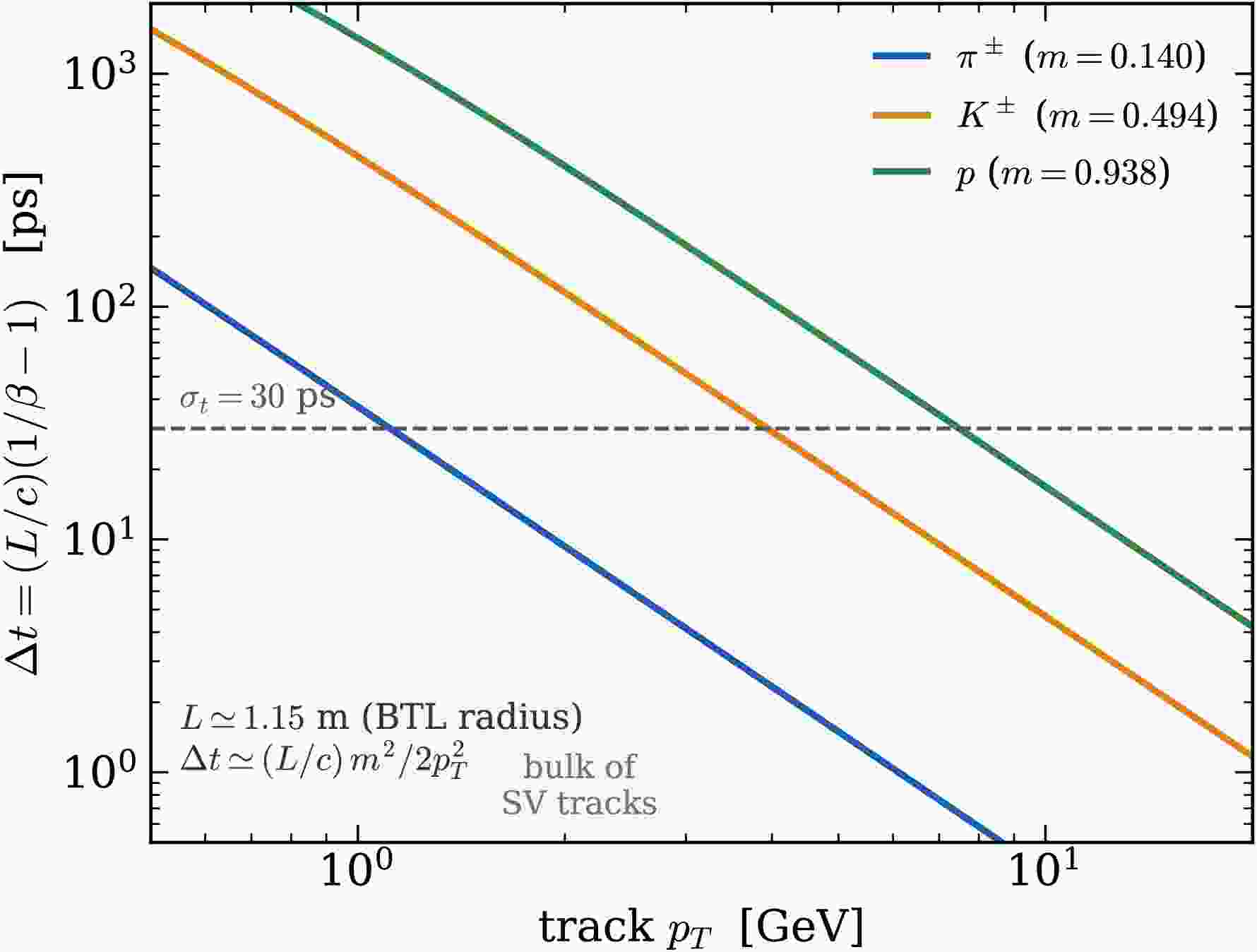
$ t_i^{{\rm{SV}}}=t_i^{{\rm{hit}}}-L_i/(\beta_i c) $ , where$ L_i $ is the helix path length from the reconstructed production point to the timing layer; in the baseline we set$ \beta_i=1 $ for the charged hadrons, and the residual bias of this approximation, which grows for the softest tracks, is varied over the track-momentum-dependent hadron-mass envelope as a systematic on the timing observables; its size as a function of track$ p_T $ and its cancellation in$ \Delta T_{{\rm{SV}}} $ are quantified in the Supplemental Material (Fig. A6). The start time$ t_0 $ is the mean production time of prompt central reference tracks ($ |d_0|<1 \,{\rm{mm}} $ ,$ |\eta|<1.48 $ ,$ p_T> 0.7 \,{\rm{GeV}} $ ); with$ {\cal{O}}(15) $ such tracks per event sharing one production time, the statistical uncertainty is$ \sigma_t/\sqrt{N} \sim 8 \;{\rm{ps}} $ . This is a statistical floor only: correlated effects— beam-spot size, detector alignment, and per-track resolution variations—do not scale as$ 1/\sqrt{N} $ and inflate the realistic per-event start-time precision toward$ \sigma_t $ itself. We therefore take$ \simeq30 \,{\rm{ps}} $ as the realistic start-time resolution throughout and quantify its impact as the Start time systematic below, where the quoted results are shown to be insensitive to this choice. A usable reference is found in 94%–96% of signal events (and in more of the high-multiplicity QCD background). The few percent of events with no prompt reference cannot define$ t_0 $ and therefore fail the 4D requirement, leaving the 3D baseline untouched. The realistic hard-scatter resolution of the barrel layer is$ \simeq30 \,{\rm{ps}} $ at start of life, rising to$ \simeq60 \,{\rm{ps}} $ at the end of operation [28]; the long-$ c\tau $ results, where the signal delay reaches hundreds of ps, are insensitive to this value, whereas the short-$ c\tau $ crossover region is not.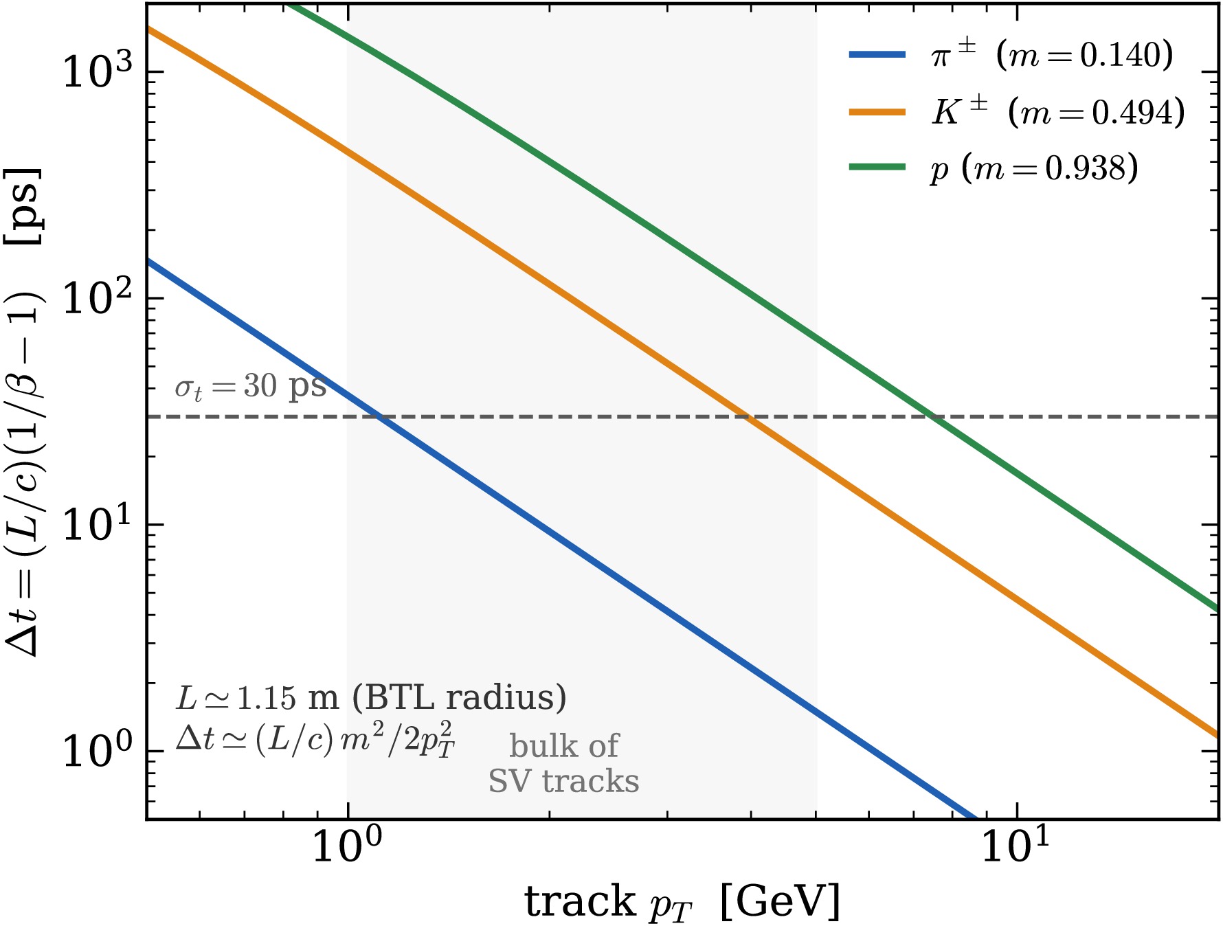
Figure A6. (color online) Per-track time bias
$ \Delta t=(L/c)(1/\beta-1) $ arising from the$ \beta=1 $ approximation, shown as a function of track$ p_T $ , for the$ \pi^\pm $ ,$ K^\pm $ , and p mass hypotheses at a barrel path length of$ L\simeq1.15\;$ m (for central tracks,$ p\simeq p_T $ ). The bias scales as$ m^2/2p_T^2 $ and is largest for low-$ p_T $ , heavy hadrons. The dashed line indicates$ \sigma_t=30 \;{\rm{ps}} $ , and the shaded band denotes the$ p_T $ range containing the bulk of the displaced-vertex tracks. Because the same approximation is applied to the prompt$ t_0 $ reference tracks, the bias is common-mode and largely cancels in$ \Delta T_{{\rm{SV}}} $ .For the selected vertex we define the time delay
$ \Delta T_{{\rm{SV}}}\equiv\langle t_i^{{\rm{SV}}}\rangle_{{\rm{SV}}}-t_0 $ , averaged over its timed tracks, and the late-track fraction$ f_{{\rm{late}}} $ , the fraction of timed vertex tracks with$ t_i^{{\rm{SV}}} $ later than$ 3 \sigma_t $ after$ t_0 $ . Because the barrel layer covers$ |\eta|<1.48 $ , only the central tracks of a vertex carry a time measurement; across the grid 80–87% of spatially selected vertices retain at least one timed track (84.9% at the benchmark$ m_s=55 \,{\rm{GeV}} $ ,$ c\tau=100 \,{\rm{mm}} $ ; see Fig. A1 in the Supplemental Material), so$ \Delta T_{{\rm{SV}}} $ is defined for the large majority, and the minority with no timed track simply fail the 4D requirement. A genuine long-lived decay produces a vertex whose tracks share a common positive delay set by the parent flight time, whereas a prompt heavy-flavour vertex is centred at$ t_0 $ ; the two observables capture, respectively, the magnitude and the coherence of the delay (Fig. 1). The nominal 4D selection requires$ \Delta T_{{\rm{SV}}}>3 \sigma_t $ and$ f_{{\rm{late}}}>0.3 $ in addition to the spatial selection. The$ f_{{\rm{late}}} $ threshold is fixed a priori at$ 0.3 $ : it demands that at least roughly one third of the timed tracks be late—enough to reject a single mistimed outlier while retaining the majority of a coherent late vertex. The gain is insensitive to this choice, changing by$ {<}$ 0.1% over$ f_{{\rm{late}}}\in[0.2,0.6] $ (Table 1). An optimized working point instead applies$ \Delta T_{{\rm{SV}}}>300 \,{\rm{ps}} $ , an illustrative tighter requirement that trades signal efficiency for a much smaller background tail.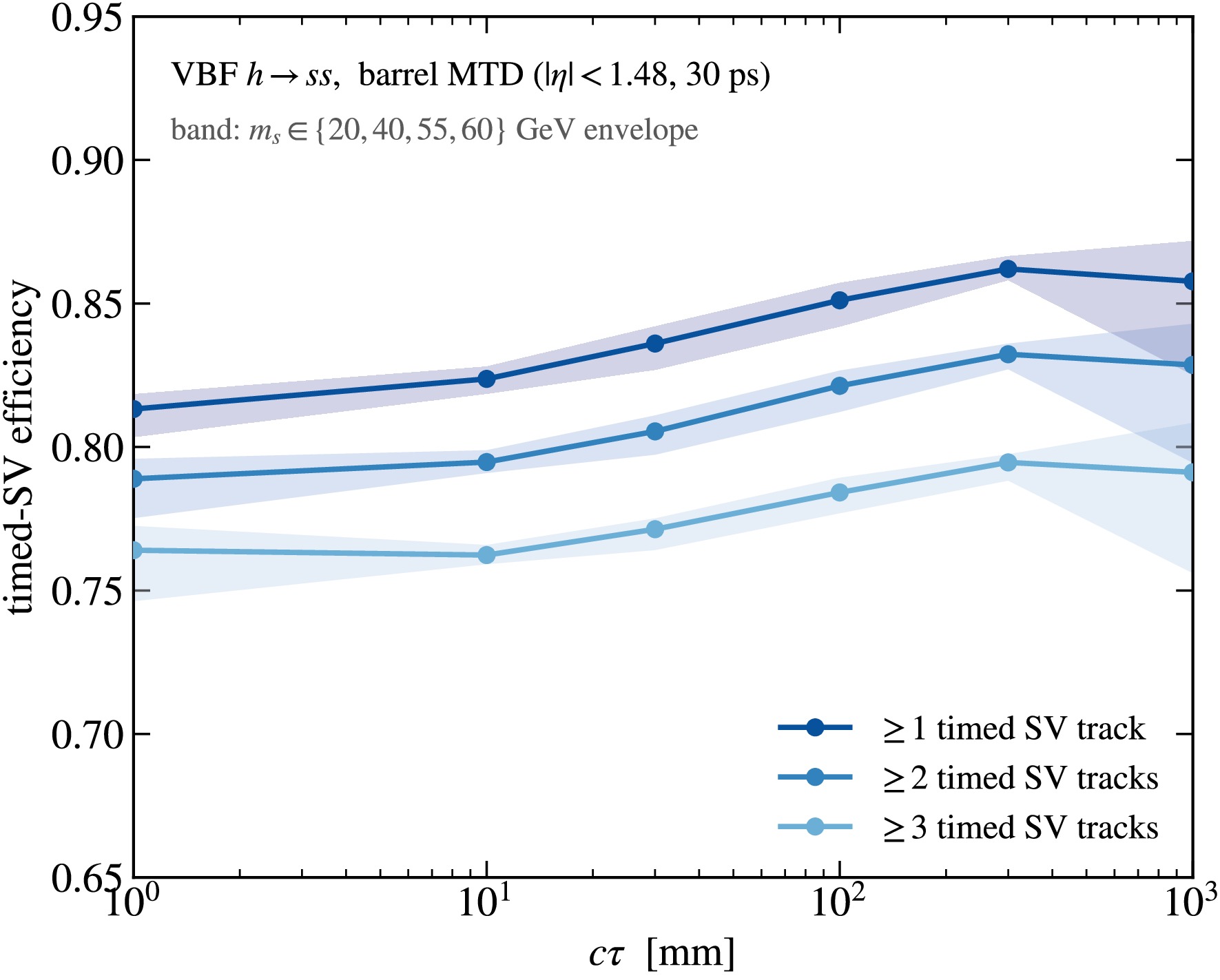
Figure A1. (color online) Fraction of spatially (3D) selected displaced vertices with at least one, two, or three SV tracks timed by the barrel layer (
$ |\eta|<1.48 $ ,$ 30 \,{\rm{ps}} $ ), as a function of decay length. Each band represents the min–max envelope across the four scalar masses,$ m_s\in\{20,40,55,60\} \,{\rm{GeV}} $ , and the line denotes the mass average.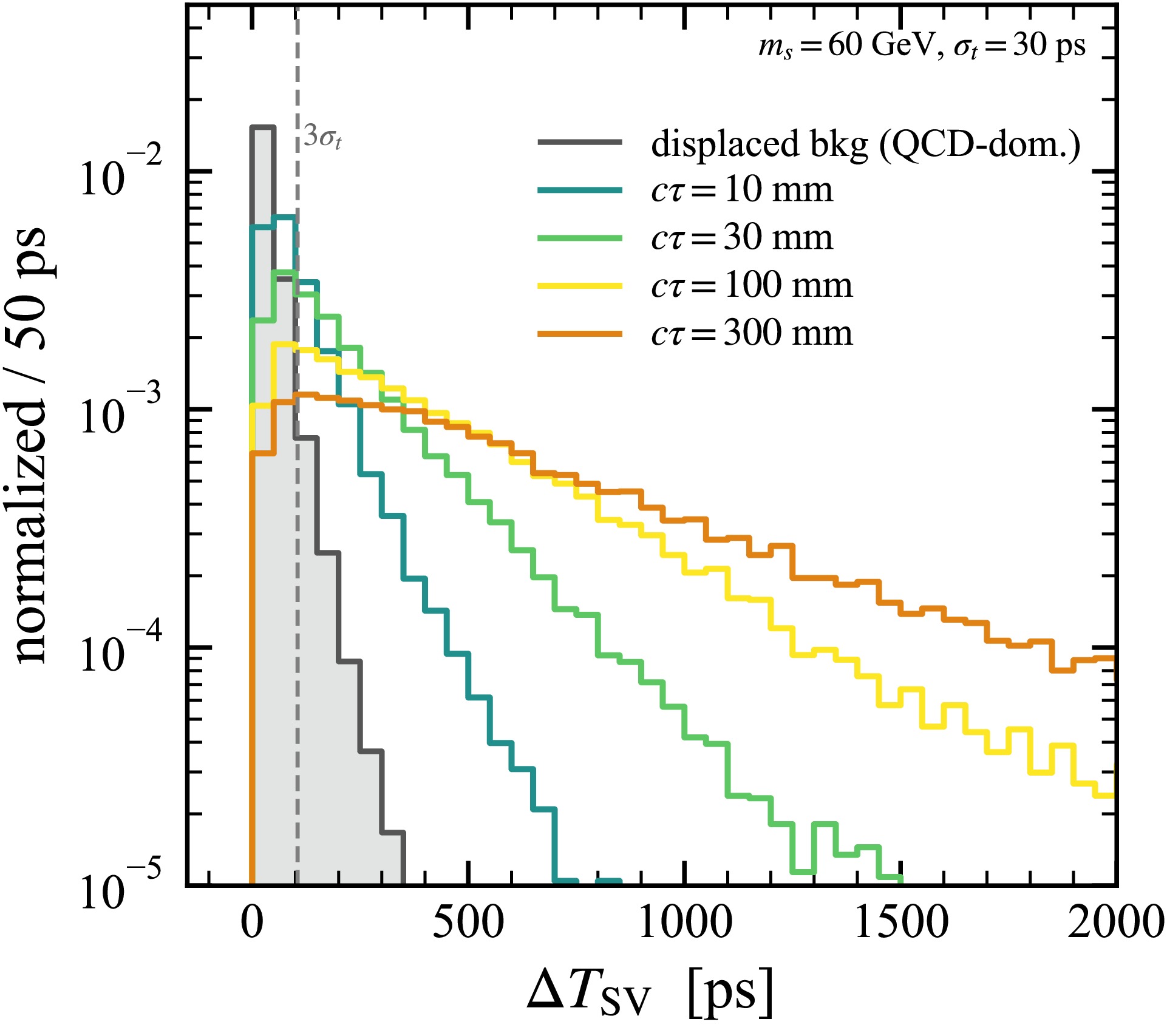
Figure 1. (color online) Normalized vertex time delay
$ \Delta T_{{\rm{SV}}} $ , constructed from path-length-corrected SV-track production times after the 3D spatial selection, for the signal at several decay lengths ($ m_s=60 \,{\rm{GeV}} $ ,$ \sigma_t=30 \,{\rm{ps}} $ ) and for the displaced background, which is dominated by QCD$ b\bar bjj $ . The background peaks at$ \Delta T_{{\rm{SV}}}\approx0 $ (prompt heavy-flavour decays at$ t_0 $ ), whereas the signal shifts to progressively larger delays as$ c\tau $ increases. The dashed line indicates the nominal$ 3 \sigma_t $ threshold.Variation $ r_S $ $ r_B $ $ {\cal{G}} $ Nominal point ( $ \Delta T_{{\rm{SV}}}>3 \sigma_t $ ,$ f_{{\rm{late}}}>0.3 $ )Baseline ( $ \sigma_t=30 \,{\rm{ps}} $ ,$ R_{{\rm{SV}}}>3 \,{\rm{mm}} $ )$ 0.755 $ $ 0.073 $ $ 2.8 $ $ \sigma_t=35 \,{\rm{ps}} $ $ 0.731 $ $ 0.051 $ $ 3.2 $ $ \sigma_t=50 \,{\rm{ps}} $ $ 0.664 $ $ 0.021 $ $ 4.6 $ $ \sigma_t=60 \,{\rm{ps}} $ $ 0.620 $ $ 0.012 $ $ 5.7 $ $ R_{{\rm{SV}}}>2 \,{\rm{mm}} $ $ 0.750 $ $ 0.063 $ $ 3.0 $ $ R_{{\rm{SV}}}>5 \,{\rm{mm}} $ $ 0.769 $ $ 0.101 $ $ 2.4 $ Optimized point ( $ \Delta T_{{\rm{SV}}}>300 \,{\rm{ps}} $ )Baseline $ 0.464 $ $ 2.1\times10^{-3} $ $ 10.2 $ $ \Delta T_{{\rm{SV}}}>150 \,{\rm{ps}} $ $ 0.664 $ $ 2.1\times10^{-2} $ $ 4.6 $ $ \Delta T_{{\rm{SV}}}>500 \,{\rm{ps}} $ (MC-stat ~20%)$ 0.276 $ $ 2.7\times10^{-4} $ $ 16.8 $ Table 1. Robustness of the timing gain at the benchmark (
$ m_s=55 \,{\rm{GeV}} $ ,$ c\tau=100 \,{\rm{mm}} $ ). Each block varies one nuisance parameter from the baseline working point;$ r_{S,B} $ are the timing-survival fractions of the spatially selected signal and (cross-section-weighted) background, and$ {\cal{G}}=r_S/\sqrt{r_B} $ . The nominal gain is stable or increases as the assumed timing resolution entering the$ 3 \sigma_t $ significance window increases, with the track-time smearing held at its start-of-life value, so the$ \sigma_t=30 \,{\rm{ps}} $ baseline is the conservative choice. It varies by$ \lesssim$ 10% across the displacement cut. To disentangle the timing resolution from the$ \sigma_t $ -scaled threshold, we replace$ \Delta T_{{\rm{SV}}}>3 \sigma_t $ with a fixed absolute threshold$ \Delta T_{{\rm{SV}}}>90 \,{\rm{ps}} $ (keeping$ f_{{\rm{late}}}>0.3 $ ):$ {\cal{G}} $ is reproduced to within 1% at every$ \sigma_t $ ($ 2.8 $ ,$ 3.2 $ ,$ 4.6 $ ,$ 5.7 $ for$ \sigma_t=30 $ –$ 60 \,{\rm{ps}} $ ). With the absolute threshold fixed, the residual$ \sigma_t $ dependence enters only through the coherence cut$ f_{{\rm{late}}} $ , whose late-track boundary is itself defined relative to$ 3 \sigma_t $ ; the near-invariance of$ {\cal{G}} $ under this replacement therefore shows that the background rejection at the nominal point is driven by$ f_{{\rm{late}}}>0.3 $ —the requirement that the delay be coherent across the vertex tracks—rather than by the absolute delay threshold. The late-track-fraction requirement is itself flat:$ {\cal{G}} $ changes by$ {<}$ 0.1% for$ f_{{\rm{late}}}\in[0.2,0.6] $ . The optimized$ \Delta T_{{\rm{SV}}}>300 \,{\rm{ps}} $ point is based on$ 200 $ raw QCD vertices ($ \simeq$ 7% Monte Carlo statistics); tighter thresholds exhaust the simulated tail and only bracket the trend. Because$ r_B $ is common to all masses, none of these variations shifts the mass pivot of Fig. 2.Because absolute yields depend on detector and pileup modeling beyond the scope of a fast simulation, we quote a normalization-free figure of merit: the ratio of the timing-enhanced sensitivity to the spatial-only sensitivity
$ {\cal{G}} \;\equiv\; \dfrac{(S/\sqrt{B})_{\rm 4D}}{(S/\sqrt{B})_{\rm 3D}} \;=\; \dfrac{r_S}{\sqrt{r_B}}, \qquad r_{S,B} \equiv \dfrac{N^{\rm 4D}_{S,B}}{N^{\rm 3D}_{S,B}}, $
(1) where
$ r_S $ and$ r_B $ are the fractions of spatially selected signal and background vertices that survive the timing requirement. The luminosity, the absolute cross sections, and any common acceptance cancel in Eq. (1):$ {\cal{G}}>1 $ indicates that the timing layer separates signal from background beyond what spatial information alone can achieve, independent of normalization. It is the robust deliverable of this work. Because$ r_S $ and$ r_B $ are constructed from the same spatial vertices in the numerator and denominator,$ {\cal{G}} $ is also independent of the timing-layer acceptance entering the 3D baseline, which is purely spatial. This 3D baseline applies the same displaced-vertex requirements as the recent ATLAS search [10]—a minimum track impact parameter, a vertex mass-to-size ratio, and a track-$ p_T $ sum—so that$ {\cal{G}} $ isolates the effect of timing on a like-for-like spatial selection; it serves as an internal reference for that purpose, not as a reproduction of the full multivariate ATLAS result. -
Each barrel-layer hit time is first converted to an estimate of the track production time,
$ t_i^{{\rm{SV}}}=t_i^{{\rm{hit}}}-L_i/(\beta_i c) $ , where$ L_i $ is the helix path length from the reconstructed production point to the timing layer; in the baseline we set$ \beta_i=1 $ for the charged hadrons, and the residual bias of this approximation, which grows for the softest tracks, is varied over the track-momentum-dependent hadron-mass envelope as a systematic on the timing observables; its size as a function of track$ p_T $ and its cancellation in$ \Delta T_{{\rm{SV}}} $ are quantified in the Supplemental Material (Fig. A6). The start time$ t_0 $ is the mean production time of prompt central reference tracks ($ |d_0|<1 \,{\rm{mm}} $ ,$ |\eta|<1.48 $ ,$ p_T> 0.7 \,{\rm{GeV}} $ ); with$ {\cal{O}}(15) $ such tracks per event sharing one production time, the statistical uncertainty is$ \sigma_t/\sqrt{N} \sim 8 \;{\rm{ps}} $ . This is a statistical floor only: correlated effects— beam-spot size, detector alignment, and per-track resolution variations—do not scale as$ 1/\sqrt{N} $ and inflate the realistic per-event start-time precision toward$ \sigma_t $ itself. We therefore take$ \simeq30 \,{\rm{ps}} $ as the realistic start-time resolution throughout and quantify its impact as the Start time systematic below, where the quoted results are shown to be insensitive to this choice. A usable reference is found in 94%–96% of signal events (and in more of the high-multiplicity QCD background). The few percent of events with no prompt reference cannot define$ t_0 $ and therefore fail the 4D requirement, leaving the 3D baseline untouched. The realistic hard-scatter resolution of the barrel layer is$ \simeq30 \,{\rm{ps}} $ at start of life, rising to$ \simeq60 \,{\rm{ps}} $ at the end of operation [28]; the long-$ c\tau $ results, where the signal delay reaches hundreds of ps, are insensitive to this value, whereas the short-$ c\tau $ crossover region is not.
Figure A6. (color online) Per-track time bias
$ \Delta t=(L/c)(1/\beta-1) $ arising from the$ \beta=1 $ approximation, shown as a function of track$ p_T $ , for the$ \pi^\pm $ ,$ K^\pm $ , and p mass hypotheses at a barrel path length of$ L\simeq1.15\;$ m (for central tracks,$ p\simeq p_T $ ). The bias scales as$ m^2/2p_T^2 $ and is largest for low-$ p_T $ , heavy hadrons. The dashed line indicates$ \sigma_t=30 \;{\rm{ps}} $ , and the shaded band denotes the$ p_T $ range containing the bulk of the displaced-vertex tracks. Because the same approximation is applied to the prompt$ t_0 $ reference tracks, the bias is common-mode and largely cancels in$ \Delta T_{{\rm{SV}}} $ .For the selected vertex we define the time delay
$ \Delta T_{{\rm{SV}}}\equiv\langle t_i^{{\rm{SV}}}\rangle_{{\rm{SV}}}-t_0 $ , averaged over its timed tracks, and the late-track fraction$ f_{{\rm{late}}} $ , the fraction of timed vertex tracks with$ t_i^{{\rm{SV}}} $ later than$ 3 \sigma_t $ after$ t_0 $ . Because the barrel layer covers$ |\eta|<1.48 $ , only the central tracks of a vertex carry a time measurement; across the grid 80–87% of spatially selected vertices retain at least one timed track (84.9% at the benchmark$ m_s=55 \,{\rm{GeV}} $ ,$ c\tau=100 \,{\rm{mm}} $ ; see Fig. A1 in the Supplemental Material), so$ \Delta T_{{\rm{SV}}} $ is defined for the large majority, and the minority with no timed track simply fail the 4D requirement. A genuine long-lived decay produces a vertex whose tracks share a common positive delay set by the parent flight time, whereas a prompt heavy-flavour vertex is centred at$ t_0 $ ; the two observables capture, respectively, the magnitude and the coherence of the delay (Fig. 1). The nominal 4D selection requires$ \Delta T_{{\rm{SV}}}>3 \sigma_t $ and$ f_{{\rm{late}}}>0.3 $ in addition to the spatial selection. The$ f_{{\rm{late}}} $ threshold is fixed a priori at$ 0.3 $ : it demands that at least roughly one third of the timed tracks be late—enough to reject a single mistimed outlier while retaining the majority of a coherent late vertex. The gain is insensitive to this choice, changing by$ {<}$ 0.1% over$ f_{{\rm{late}}}\in[0.2,0.6] $ (Table 1). An optimized working point instead applies$ \Delta T_{{\rm{SV}}}>300 \,{\rm{ps}} $ , an illustrative tighter requirement that trades signal efficiency for a much smaller background tail.
Figure A1. (color online) Fraction of spatially (3D) selected displaced vertices with at least one, two, or three SV tracks timed by the barrel layer (
$ |\eta|<1.48 $ ,$ 30 \,{\rm{ps}} $ ), as a function of decay length. Each band represents the min–max envelope across the four scalar masses,$ m_s\in\{20,40,55,60\} \,{\rm{GeV}} $ , and the line denotes the mass average.
Figure 1. (color online) Normalized vertex time delay
$ \Delta T_{{\rm{SV}}} $ , constructed from path-length-corrected SV-track production times after the 3D spatial selection, for the signal at several decay lengths ($ m_s=60 \,{\rm{GeV}} $ ,$ \sigma_t=30 \,{\rm{ps}} $ ) and for the displaced background, which is dominated by QCD$ b\bar bjj $ . The background peaks at$ \Delta T_{{\rm{SV}}}\approx0 $ (prompt heavy-flavour decays at$ t_0 $ ), whereas the signal shifts to progressively larger delays as$ c\tau $ increases. The dashed line indicates the nominal$ 3 \sigma_t $ threshold.Variation $ r_S $ $ r_B $ $ {\cal{G}} $ Nominal point ( $ \Delta T_{{\rm{SV}}}>3 \sigma_t $ ,$ f_{{\rm{late}}}>0.3 $ )Baseline ( $ \sigma_t=30 \,{\rm{ps}} $ ,$ R_{{\rm{SV}}}>3 \,{\rm{mm}} $ )$ 0.755 $ $ 0.073 $ $ 2.8 $ $ \sigma_t=35 \,{\rm{ps}} $ $ 0.731 $ $ 0.051 $ $ 3.2 $ $ \sigma_t=50 \,{\rm{ps}} $ $ 0.664 $ $ 0.021 $ $ 4.6 $ $ \sigma_t=60 \,{\rm{ps}} $ $ 0.620 $ $ 0.012 $ $ 5.7 $ $ R_{{\rm{SV}}}>2 \,{\rm{mm}} $ $ 0.750 $ $ 0.063 $ $ 3.0 $ $ R_{{\rm{SV}}}>5 \,{\rm{mm}} $ $ 0.769 $ $ 0.101 $ $ 2.4 $ Optimized point ( $ \Delta T_{{\rm{SV}}}>300 \,{\rm{ps}} $ )Baseline $ 0.464 $ $ 2.1\times10^{-3} $ $ 10.2 $ $ \Delta T_{{\rm{SV}}}>150 \,{\rm{ps}} $ $ 0.664 $ $ 2.1\times10^{-2} $ $ 4.6 $ $ \Delta T_{{\rm{SV}}}>500 \,{\rm{ps}} $ (MC-stat ~20%)$ 0.276 $ $ 2.7\times10^{-4} $ $ 16.8 $ Table 1. Robustness of the timing gain at the benchmark (
$ m_s=55 \,{\rm{GeV}} $ ,$ c\tau=100 \,{\rm{mm}} $ ). Each block varies one nuisance parameter from the baseline working point;$ r_{S,B} $ are the timing-survival fractions of the spatially selected signal and (cross-section-weighted) background, and$ {\cal{G}}=r_S/\sqrt{r_B} $ . The nominal gain is stable or increases as the assumed timing resolution entering the$ 3 \sigma_t $ significance window increases, with the track-time smearing held at its start-of-life value, so the$ \sigma_t=30 \,{\rm{ps}} $ baseline is the conservative choice. It varies by$ \lesssim$ 10% across the displacement cut. To disentangle the timing resolution from the$ \sigma_t $ -scaled threshold, we replace$ \Delta T_{{\rm{SV}}}>3 \sigma_t $ with a fixed absolute threshold$ \Delta T_{{\rm{SV}}}>90 \,{\rm{ps}} $ (keeping$ f_{{\rm{late}}}>0.3 $ ):$ {\cal{G}} $ is reproduced to within 1% at every$ \sigma_t $ ($ 2.8 $ ,$ 3.2 $ ,$ 4.6 $ ,$ 5.7 $ for$ \sigma_t=30 $ –$ 60 \,{\rm{ps}} $ ). With the absolute threshold fixed, the residual$ \sigma_t $ dependence enters only through the coherence cut$ f_{{\rm{late}}} $ , whose late-track boundary is itself defined relative to$ 3 \sigma_t $ ; the near-invariance of$ {\cal{G}} $ under this replacement therefore shows that the background rejection at the nominal point is driven by$ f_{{\rm{late}}}>0.3 $ —the requirement that the delay be coherent across the vertex tracks—rather than by the absolute delay threshold. The late-track-fraction requirement is itself flat:$ {\cal{G}} $ changes by$ {<}$ 0.1% for$ f_{{\rm{late}}}\in[0.2,0.6] $ . The optimized$ \Delta T_{{\rm{SV}}}>300 \,{\rm{ps}} $ point is based on$ 200 $ raw QCD vertices ($ \simeq$ 7% Monte Carlo statistics); tighter thresholds exhaust the simulated tail and only bracket the trend. Because$ r_B $ is common to all masses, none of these variations shifts the mass pivot of Fig. 2.Because absolute yields depend on detector and pileup modeling beyond the scope of a fast simulation, we quote a normalization-free figure of merit: the ratio of the timing-enhanced sensitivity to the spatial-only sensitivity
$ {\cal{G}} \;\equiv\; \dfrac{(S/\sqrt{B})_{\rm 4D}}{(S/\sqrt{B})_{\rm 3D}} \;=\; \dfrac{r_S}{\sqrt{r_B}}, \qquad r_{S,B} \equiv \dfrac{N^{\rm 4D}_{S,B}}{N^{\rm 3D}_{S,B}}, $
(1) where
$ r_S $ and$ r_B $ are the fractions of spatially selected signal and background vertices that survive the timing requirement. The luminosity, the absolute cross sections, and any common acceptance cancel in Eq. (1):$ {\cal{G}}>1 $ indicates that the timing layer separates signal from background beyond what spatial information alone can achieve, independent of normalization. It is the robust deliverable of this work. Because$ r_S $ and$ r_B $ are constructed from the same spatial vertices in the numerator and denominator,$ {\cal{G}} $ is also independent of the timing-layer acceptance entering the 3D baseline, which is purely spatial. This 3D baseline applies the same displaced-vertex requirements as the recent ATLAS search [10]—a minimum track impact parameter, a vertex mass-to-size ratio, and a track-$ p_T $ sum—so that$ {\cal{G}} $ isolates the effect of timing on a like-for-like spatial selection; it serves as an internal reference for that purpose, not as a reproduction of the full multivariate ATLAS result. -
Each barrel-layer hit time is first converted to an estimate of the track production time,
$ t_i^{{\rm{SV}}}=t_i^{{\rm{hit}}}-L_i/(\beta_i c) $ , where$ L_i $ is the helix path length from the reconstructed production point to the timing layer; in the baseline we set$ \beta_i=1 $ for the charged hadrons, and the residual bias of this approximation, which grows for the softest tracks, is varied over the track-momentum-dependent hadron-mass envelope as a systematic on the timing observables; its size as a function of track$ p_T $ and its cancellation in$ \Delta T_{{\rm{SV}}} $ are quantified in the Supplemental Material (Fig. A6). The start time$ t_0 $ is the mean production time of prompt central reference tracks ($ |d_0|<1 \,{\rm{mm}} $ ,$ |\eta|<1.48 $ ,$ p_T> 0.7 \,{\rm{GeV}} $ ); with$ {\cal{O}}(15) $ such tracks per event sharing one production time, the statistical uncertainty is$ \sigma_t/\sqrt{N} \sim 8 \;{\rm{ps}} $ . This is a statistical floor only: correlated effects— beam-spot size, detector alignment, and per-track resolution variations—do not scale as$ 1/\sqrt{N} $ and inflate the realistic per-event start-time precision toward$ \sigma_t $ itself. We therefore take$ \simeq30 \,{\rm{ps}} $ as the realistic start-time resolution throughout and quantify its impact as the Start time systematic below, where the quoted results are shown to be insensitive to this choice. A usable reference is found in 94%–96% of signal events (and in more of the high-multiplicity QCD background). The few percent of events with no prompt reference cannot define$ t_0 $ and therefore fail the 4D requirement, leaving the 3D baseline untouched. The realistic hard-scatter resolution of the barrel layer is$ \simeq30 \,{\rm{ps}} $ at start of life, rising to$ \simeq60 \,{\rm{ps}} $ at the end of operation [28]; the long-$ c\tau $ results, where the signal delay reaches hundreds of ps, are insensitive to this value, whereas the short-$ c\tau $ crossover region is not.
Figure A6. (color online) Per-track time bias
$ \Delta t=(L/c)(1/\beta-1) $ arising from the$ \beta=1 $ approximation, shown as a function of track$ p_T $ , for the$ \pi^\pm $ ,$ K^\pm $ , and p mass hypotheses at a barrel path length of$ L\simeq1.15\;$ m (for central tracks,$ p\simeq p_T $ ). The bias scales as$ m^2/2p_T^2 $ and is largest for low-$ p_T $ , heavy hadrons. The dashed line indicates$ \sigma_t=30 \;{\rm{ps}} $ , and the shaded band denotes the$ p_T $ range containing the bulk of the displaced-vertex tracks. Because the same approximation is applied to the prompt$ t_0 $ reference tracks, the bias is common-mode and largely cancels in$ \Delta T_{{\rm{SV}}} $ .For the selected vertex we define the time delay
$ \Delta T_{{\rm{SV}}}\equiv\langle t_i^{{\rm{SV}}}\rangle_{{\rm{SV}}}-t_0 $ , averaged over its timed tracks, and the late-track fraction$ f_{{\rm{late}}} $ , the fraction of timed vertex tracks with$ t_i^{{\rm{SV}}} $ later than$ 3 \sigma_t $ after$ t_0 $ . Because the barrel layer covers$ |\eta|<1.48 $ , only the central tracks of a vertex carry a time measurement; across the grid 80–87% of spatially selected vertices retain at least one timed track (84.9% at the benchmark$ m_s=55 \,{\rm{GeV}} $ ,$ c\tau=100 \,{\rm{mm}} $ ; see Fig. A1 in the Supplemental Material), so$ \Delta T_{{\rm{SV}}} $ is defined for the large majority, and the minority with no timed track simply fail the 4D requirement. A genuine long-lived decay produces a vertex whose tracks share a common positive delay set by the parent flight time, whereas a prompt heavy-flavour vertex is centred at$ t_0 $ ; the two observables capture, respectively, the magnitude and the coherence of the delay (Fig. 1). The nominal 4D selection requires$ \Delta T_{{\rm{SV}}}>3 \sigma_t $ and$ f_{{\rm{late}}}>0.3 $ in addition to the spatial selection. The$ f_{{\rm{late}}} $ threshold is fixed a priori at$ 0.3 $ : it demands that at least roughly one third of the timed tracks be late—enough to reject a single mistimed outlier while retaining the majority of a coherent late vertex. The gain is insensitive to this choice, changing by$ {<}$ 0.1% over$ f_{{\rm{late}}}\in[0.2,0.6] $ (Table 1). An optimized working point instead applies$ \Delta T_{{\rm{SV}}}>300 \,{\rm{ps}} $ , an illustrative tighter requirement that trades signal efficiency for a much smaller background tail.
Figure A1. (color online) Fraction of spatially (3D) selected displaced vertices with at least one, two, or three SV tracks timed by the barrel layer (
$ |\eta|<1.48 $ ,$ 30 \,{\rm{ps}} $ ), as a function of decay length. Each band represents the min–max envelope across the four scalar masses,$ m_s\in\{20,40,55,60\} \,{\rm{GeV}} $ , and the line denotes the mass average.
Figure 1. (color online) Normalized vertex time delay
$ \Delta T_{{\rm{SV}}} $ , constructed from path-length-corrected SV-track production times after the 3D spatial selection, for the signal at several decay lengths ($ m_s=60 \,{\rm{GeV}} $ ,$ \sigma_t=30 \,{\rm{ps}} $ ) and for the displaced background, which is dominated by QCD$ b\bar bjj $ . The background peaks at$ \Delta T_{{\rm{SV}}}\approx0 $ (prompt heavy-flavour decays at$ t_0 $ ), whereas the signal shifts to progressively larger delays as$ c\tau $ increases. The dashed line indicates the nominal$ 3 \sigma_t $ threshold.Variation $ r_S $ $ r_B $ $ {\cal{G}} $ Nominal point ( $ \Delta T_{{\rm{SV}}}>3 \sigma_t $ ,$ f_{{\rm{late}}}>0.3 $ )Baseline ( $ \sigma_t=30 \,{\rm{ps}} $ ,$ R_{{\rm{SV}}}>3 \,{\rm{mm}} $ )$ 0.755 $ $ 0.073 $ $ 2.8 $ $ \sigma_t=35 \,{\rm{ps}} $ $ 0.731 $ $ 0.051 $ $ 3.2 $ $ \sigma_t=50 \,{\rm{ps}} $ $ 0.664 $ $ 0.021 $ $ 4.6 $ $ \sigma_t=60 \,{\rm{ps}} $ $ 0.620 $ $ 0.012 $ $ 5.7 $ $ R_{{\rm{SV}}}>2 \,{\rm{mm}} $ $ 0.750 $ $ 0.063 $ $ 3.0 $ $ R_{{\rm{SV}}}>5 \,{\rm{mm}} $ $ 0.769 $ $ 0.101 $ $ 2.4 $ Optimized point ( $ \Delta T_{{\rm{SV}}}>300 \,{\rm{ps}} $ )Baseline $ 0.464 $ $ 2.1\times10^{-3} $ $ 10.2 $ $ \Delta T_{{\rm{SV}}}>150 \,{\rm{ps}} $ $ 0.664 $ $ 2.1\times10^{-2} $ $ 4.6 $ $ \Delta T_{{\rm{SV}}}>500 \,{\rm{ps}} $ (MC-stat ~20%)$ 0.276 $ $ 2.7\times10^{-4} $ $ 16.8 $ Table 1. Robustness of the timing gain at the benchmark (
$ m_s=55 \,{\rm{GeV}} $ ,$ c\tau=100 \,{\rm{mm}} $ ). Each block varies one nuisance parameter from the baseline working point;$ r_{S,B} $ are the timing-survival fractions of the spatially selected signal and (cross-section-weighted) background, and$ {\cal{G}}=r_S/\sqrt{r_B} $ . The nominal gain is stable or increases as the assumed timing resolution entering the$ 3 \sigma_t $ significance window increases, with the track-time smearing held at its start-of-life value, so the$ \sigma_t=30 \,{\rm{ps}} $ baseline is the conservative choice. It varies by$ \lesssim$ 10% across the displacement cut. To disentangle the timing resolution from the$ \sigma_t $ -scaled threshold, we replace$ \Delta T_{{\rm{SV}}}>3 \sigma_t $ with a fixed absolute threshold$ \Delta T_{{\rm{SV}}}>90 \,{\rm{ps}} $ (keeping$ f_{{\rm{late}}}>0.3 $ ):$ {\cal{G}} $ is reproduced to within 1% at every$ \sigma_t $ ($ 2.8 $ ,$ 3.2 $ ,$ 4.6 $ ,$ 5.7 $ for$ \sigma_t=30 $ –$ 60 \,{\rm{ps}} $ ). With the absolute threshold fixed, the residual$ \sigma_t $ dependence enters only through the coherence cut$ f_{{\rm{late}}} $ , whose late-track boundary is itself defined relative to$ 3 \sigma_t $ ; the near-invariance of$ {\cal{G}} $ under this replacement therefore shows that the background rejection at the nominal point is driven by$ f_{{\rm{late}}}>0.3 $ —the requirement that the delay be coherent across the vertex tracks—rather than by the absolute delay threshold. The late-track-fraction requirement is itself flat:$ {\cal{G}} $ changes by$ {<}$ 0.1% for$ f_{{\rm{late}}}\in[0.2,0.6] $ . The optimized$ \Delta T_{{\rm{SV}}}>300 \,{\rm{ps}} $ point is based on$ 200 $ raw QCD vertices ($ \simeq$ 7% Monte Carlo statistics); tighter thresholds exhaust the simulated tail and only bracket the trend. Because$ r_B $ is common to all masses, none of these variations shifts the mass pivot of Fig. 2.Because absolute yields depend on detector and pileup modeling beyond the scope of a fast simulation, we quote a normalization-free figure of merit: the ratio of the timing-enhanced sensitivity to the spatial-only sensitivity
$ {\cal{G}} \;\equiv\; \dfrac{(S/\sqrt{B})_{\rm 4D}}{(S/\sqrt{B})_{\rm 3D}} \;=\; \dfrac{r_S}{\sqrt{r_B}}, \qquad r_{S,B} \equiv \dfrac{N^{\rm 4D}_{S,B}}{N^{\rm 3D}_{S,B}}, $
(1) where
$ r_S $ and$ r_B $ are the fractions of spatially selected signal and background vertices that survive the timing requirement. The luminosity, the absolute cross sections, and any common acceptance cancel in Eq. (1):$ {\cal{G}}>1 $ indicates that the timing layer separates signal from background beyond what spatial information alone can achieve, independent of normalization. It is the robust deliverable of this work. Because$ r_S $ and$ r_B $ are constructed from the same spatial vertices in the numerator and denominator,$ {\cal{G}} $ is also independent of the timing-layer acceptance entering the 3D baseline, which is purely spatial. This 3D baseline applies the same displaced-vertex requirements as the recent ATLAS search [10]—a minimum track impact parameter, a vertex mass-to-size ratio, and a track-$ p_T $ sum—so that$ {\cal{G}} $ isolates the effect of timing on a like-for-like spatial selection; it serves as an internal reference for that purpose, not as a reproduction of the full multivariate ATLAS result. -
The dominant irreducible background is the prompt production of displaced-vertex candidates from heavy-flavour decays. We generate three contributions, each normalized by its own generated cross section: QCD
$ b\bar bjj $ ($ 540 \,{\rm{pb}} $ ), electroweak$ b\bar bjj $ ($ 0.21 \,{\rm{pb}} $ ), and SM VBF$ h\to b\bar b $ ($ 0.17 \,{\rm{pb}} $ ). After selection, the total is dominated by QCD$ b\bar bjj $ , which supplies 99.9% of the spatially selected background because its cross section exceeds those of the other contributions by three orders of magnitude. All three are time-prompt: their vertices arise from b- and c-hadron decays at the hard-scatter time, populating$ \Delta T_{{\rm{SV}}}\approx0 $ (median$ 25 \;{\rm{ps}} $ , median$ R_{{\rm{SV}}}=5 \;{\rm{mm}} $ ). Because these vertices peak at$ \Delta T_{{\rm{SV}}}\approx0 $ , the late-time tail on which the timing selection acts is populated by the detector timing response and by pileup, not by the tail of the QCD matrix element. The leading-order simulation therefore determines this tail shape only approximately; in a real analysis, it would be constrained by the$ \Delta T_{{\rm{SV}}}<0 $ sideband—which mirrors the prompt timing response— rather than by the perturbative order of the calculation. This is the physical origin of the timing discrimination: the background that survives the spatial selection is precisely the population that the timing layer is designed to reject, and the QCD continuum is even more prompt than SM$ h\to b\bar b $ (timing survival 7% versus 11%). Fully hadronic$ t\bar t $ production yields a similar b-rich multijet final state and can in principle populate the selection, but the forward, high-mass VBF dijet requirement strongly suppresses its central topology, leaving it subdominant to the QCD continuum and, being equally time-prompt, subject to the same timing rejection. Other displaced or instrumental backgrounds fall into two classes. Photon conversions, hadronic material interactions, and fake or pileup-combinatorial vertices are prompt in collision time and are suppressed, not enhanced, by the timing requirement—with the random-late pileup component bracketed by the Pileup systematic below.$ K^0_S $ and Λ decays, by contrast, are genuinely late: with proper decay lengths$ c\tau=26.8 $ and$ 79 \,{\rm{mm}} $ , they carry true flight-time delays and would not be rejected by timing. They are instead removed before the timing step by the spatial selection, because a$ V^0 $ is a two-prong, low-mass object ($ m_{K^0_S}=0.498 $ ,$ m_\Lambda=1.116 \,{\rm{GeV}} $ ) that fails both the$ \geqslant3 $ -track requirement and the$ m_{{\rm{SV}}}/\Delta R>4 \,{\rm{GeV}} $ mass-to-size cut, whereas signal vertices carry masses of tens of GeV. For a$ V^0 $ to enter the 3D selection, it would need to acquire additional tracks accidentally and reach a vertex mass an order of magnitude above that of the parent—a combinatorially negligible configuration—so we bound the$ V^0 $ contribution to the spatially selected background, and hence to$ r_B $ and$ {\cal{G}} $ , at the sub-percent level. A fast simulation cannot model these instrumental components reliably; a real analysis controls them with material vetoes,$ V^0 $ mass tags, and a data-driven background estimate [10, 12]. To first approximation, they enter as a normalization or tail-shape uncertainty on the prompt background rather than as a genuine late population—an assumption that only collision data can validate through dedicated control regions: the$ \Delta T_{{\rm{SV}}}<0 $ sideband to calibrate the prompt timing response and its tail, a low-$ m_{{\rm{SV}}}/\Delta R $ or low-$ \displaystyle\sum p_T $ region to enrich prompt heavy-flavour vertices, a VBF sideband at lower$ m_{jj} $ or$ |\Delta\eta_{jj}| $ to control the QCD continuum, and random-crossing overlays to assess the pileup-combinatorial tail. Their residual effect is confined to the absolute normalization, which we bracket through$ \kappa_b $ , and does not alter the gain$ {\cal{G}} $ . -
The dominant irreducible background is the prompt production of displaced-vertex candidates from heavy-flavour decays. We generate three contributions, each normalized by its own generated cross section: QCD
$ b\bar bjj $ ($ 540 \,{\rm{pb}} $ ), electroweak$ b\bar bjj $ ($ 0.21 \,{\rm{pb}} $ ), and SM VBF$ h\to b\bar b $ ($ 0.17 \,{\rm{pb}} $ ). After selection, the total is dominated by QCD$ b\bar bjj $ , which supplies 99.9% of the spatially selected background because its cross section exceeds those of the other contributions by three orders of magnitude. All three are time-prompt: their vertices arise from b- and c-hadron decays at the hard-scatter time, populating$ \Delta T_{{\rm{SV}}}\approx0 $ (median$ 25 \;{\rm{ps}} $ , median$ R_{{\rm{SV}}}=5 \;{\rm{mm}} $ ). Because these vertices peak at$ \Delta T_{{\rm{SV}}}\approx0 $ , the late-time tail on which the timing selection acts is populated by the detector timing response and by pileup, not by the tail of the QCD matrix element. The leading-order simulation therefore determines this tail shape only approximately; in a real analysis, it would be constrained by the$ \Delta T_{{\rm{SV}}}<0 $ sideband—which mirrors the prompt timing response— rather than by the perturbative order of the calculation. This is the physical origin of the timing discrimination: the background that survives the spatial selection is precisely the population that the timing layer is designed to reject, and the QCD continuum is even more prompt than SM$ h\to b\bar b $ (timing survival 7% versus 11%). Fully hadronic$ t\bar t $ production yields a similar b-rich multijet final state and can in principle populate the selection, but the forward, high-mass VBF dijet requirement strongly suppresses its central topology, leaving it subdominant to the QCD continuum and, being equally time-prompt, subject to the same timing rejection. Other displaced or instrumental backgrounds fall into two classes. Photon conversions, hadronic material interactions, and fake or pileup-combinatorial vertices are prompt in collision time and are suppressed, not enhanced, by the timing requirement—with the random-late pileup component bracketed by the Pileup systematic below.$ K^0_S $ and Λ decays, by contrast, are genuinely late: with proper decay lengths$ c\tau=26.8 $ and$ 79 \,{\rm{mm}} $ , they carry true flight-time delays and would not be rejected by timing. They are instead removed before the timing step by the spatial selection, because a$ V^0 $ is a two-prong, low-mass object ($ m_{K^0_S}=0.498 $ ,$ m_\Lambda=1.116 \,{\rm{GeV}} $ ) that fails both the$ \geqslant3 $ -track requirement and the$ m_{{\rm{SV}}}/\Delta R>4 \,{\rm{GeV}} $ mass-to-size cut, whereas signal vertices carry masses of tens of GeV. For a$ V^0 $ to enter the 3D selection, it would need to acquire additional tracks accidentally and reach a vertex mass an order of magnitude above that of the parent—a combinatorially negligible configuration—so we bound the$ V^0 $ contribution to the spatially selected background, and hence to$ r_B $ and$ {\cal{G}} $ , at the sub-percent level. A fast simulation cannot model these instrumental components reliably; a real analysis controls them with material vetoes,$ V^0 $ mass tags, and a data-driven background estimate [10, 12]. To first approximation, they enter as a normalization or tail-shape uncertainty on the prompt background rather than as a genuine late population—an assumption that only collision data can validate through dedicated control regions: the$ \Delta T_{{\rm{SV}}}<0 $ sideband to calibrate the prompt timing response and its tail, a low-$ m_{{\rm{SV}}}/\Delta R $ or low-$ \displaystyle\sum p_T $ region to enrich prompt heavy-flavour vertices, a VBF sideband at lower$ m_{jj} $ or$ |\Delta\eta_{jj}| $ to control the QCD continuum, and random-crossing overlays to assess the pileup-combinatorial tail. Their residual effect is confined to the absolute normalization, which we bracket through$ \kappa_b $ , and does not alter the gain$ {\cal{G}} $ . -
The dominant irreducible background is the prompt production of displaced-vertex candidates from heavy-flavour decays. We generate three contributions, each normalized by its own generated cross section: QCD
$ b\bar bjj $ ($ 540 \,{\rm{pb}} $ ), electroweak$ b\bar bjj $ ($ 0.21 \,{\rm{pb}} $ ), and SM VBF$ h\to b\bar b $ ($ 0.17 \,{\rm{pb}} $ ). After selection, the total is dominated by QCD$ b\bar bjj $ , which supplies 99.9% of the spatially selected background because its cross section exceeds those of the other contributions by three orders of magnitude. All three are time-prompt: their vertices arise from b- and c-hadron decays at the hard-scatter time, populating$ \Delta T_{{\rm{SV}}}\approx0 $ (median$ 25 \;{\rm{ps}} $ , median$ R_{{\rm{SV}}}=5 \;{\rm{mm}} $ ). Because these vertices peak at$ \Delta T_{{\rm{SV}}}\approx0 $ , the late-time tail on which the timing selection acts is populated by the detector timing response and by pileup, not by the tail of the QCD matrix element. The leading-order simulation therefore determines this tail shape only approximately; in a real analysis, it would be constrained by the$ \Delta T_{{\rm{SV}}}<0 $ sideband—which mirrors the prompt timing response— rather than by the perturbative order of the calculation. This is the physical origin of the timing discrimination: the background that survives the spatial selection is precisely the population that the timing layer is designed to reject, and the QCD continuum is even more prompt than SM$ h\to b\bar b $ (timing survival 7% versus 11%). Fully hadronic$ t\bar t $ production yields a similar b-rich multijet final state and can in principle populate the selection, but the forward, high-mass VBF dijet requirement strongly suppresses its central topology, leaving it subdominant to the QCD continuum and, being equally time-prompt, subject to the same timing rejection. Other displaced or instrumental backgrounds fall into two classes. Photon conversions, hadronic material interactions, and fake or pileup-combinatorial vertices are prompt in collision time and are suppressed, not enhanced, by the timing requirement—with the random-late pileup component bracketed by the Pileup systematic below.$ K^0_S $ and Λ decays, by contrast, are genuinely late: with proper decay lengths$ c\tau=26.8 $ and$ 79 \,{\rm{mm}} $ , they carry true flight-time delays and would not be rejected by timing. They are instead removed before the timing step by the spatial selection, because a$ V^0 $ is a two-prong, low-mass object ($ m_{K^0_S}=0.498 $ ,$ m_\Lambda=1.116 \,{\rm{GeV}} $ ) that fails both the$ \geqslant3 $ -track requirement and the$ m_{{\rm{SV}}}/\Delta R>4 \,{\rm{GeV}} $ mass-to-size cut, whereas signal vertices carry masses of tens of GeV. For a$ V^0 $ to enter the 3D selection, it would need to acquire additional tracks accidentally and reach a vertex mass an order of magnitude above that of the parent—a combinatorially negligible configuration—so we bound the$ V^0 $ contribution to the spatially selected background, and hence to$ r_B $ and$ {\cal{G}} $ , at the sub-percent level. A fast simulation cannot model these instrumental components reliably; a real analysis controls them with material vetoes,$ V^0 $ mass tags, and a data-driven background estimate [10, 12]. To first approximation, they enter as a normalization or tail-shape uncertainty on the prompt background rather than as a genuine late population—an assumption that only collision data can validate through dedicated control regions: the$ \Delta T_{{\rm{SV}}}<0 $ sideband to calibrate the prompt timing response and its tail, a low-$ m_{{\rm{SV}}}/\Delta R $ or low-$ \displaystyle\sum p_T $ region to enrich prompt heavy-flavour vertices, a VBF sideband at lower$ m_{jj} $ or$ |\Delta\eta_{jj}| $ to control the QCD continuum, and random-crossing overlays to assess the pileup-combinatorial tail. Their residual effect is confined to the absolute normalization, which we bracket through$ \kappa_b $ , and does not alter the gain$ {\cal{G}} $ . -
The timing layer acts almost exclusively on the background (Table A1 in the Supplemental Material): across the grid, it retains
$ r_B=0.073 $ of the spatially selected background at the nominal point and$ r_B=2.1\times10^{-3} $ at the optimized point, while retaining 60%$ \text{–}$ 80% of the signal for$ c\tau\gtrsim30 \,{\rm{mm}} $ . Through Eq. (1), this yields a gain of$ {\cal{G}}=2.8 $ at the nominal working point and$ {\cal{G}}\simeq10 $ at the optimized point for the benchmark$ m_s=60 \;{\rm{GeV}} $ ,$ c\tau=100 \;{\rm{mm}} $ , rising to$ {\cal{G}}\simeq15 $ at$ c\tau=1000 \;{\rm{mm}} $ , where essentially all of the signal is delayed but the prompt background is fully rejected. For$ c\tau\lesssim10 \;{\rm{mm}} $ , the gain falls below unity: the signal delay becomes comparable to$ \sigma_t $ , so the timing cut discards signal without a compensating reduction in background, and the spatial selection alone is preferable.Selection stage Signal QCD $ b\bar bjj $ Generated 200000 2200000 VBF tag jets 53993 369534 $ \geqslant3 $ displaced tracks53884 322922 Displaced vertex ( $ \geqslant3 $ trk,$ R_{{\rm{SV}}}>3 \,{\rm{mm}} $ )39237 122288 $ \displaystyle\sum p_T>10 \,{\rm{GeV}} $ 33583 101500 $ m_{{\rm{SV}}}/\Delta R>4 $ (3D)32145 96435 $ + $ 4D timing (nominal)24276 7021 $ +\ \Delta T_{{\rm{SV}}}>300 \,{\rm{ps}} $ (opt.)14916 200 Table A1. Cutflow for a representative signal benchmark (
$ m_s=55 \,{\rm{GeV}} $ ,$ c\tau=100 \,{\rm{mm}} $ ,$ 2\times10^{5} $ generated events) and the dominant QCD$ b\bar bjj $ background ($ 2.2\times10^{6} $ generated events). The 3D selection terminates at the$ m_{{\rm{SV}}}/\Delta R $ cut; "4D" additionally applies the nominal timing requirement, and "$ \Delta T_{{\rm{SV}}}>300 $ " applies the optimized one. The larger QCD sample sets the statistical precision of the optimized late-time count to$ \simeq$ 7%. The timing layer rejects 93% of the spatially selected QCD vertices and 24% of the signal, consistent with the quantitative content of Eq. (1).The dependence on scalar mass, shown in Fig. 2, is the central structural result. As anticipated from the kinematics—the lab-frame decay length is
$ L_{{\rm{lab}}}\simeq\beta\gamma\, c\tau $ with$ \beta\gamma\simeq p_s/ m_s $ , so the mean boost scales as$ \langle\gamma_s\rangle\propto1/ m_s $ and lighter scalars travel farther for a given proper lifetime— the two mass regimes trade places at a well-defined decay length. At short$ c\tau $ , the larger boost of the light scalar pushes more decays beyond the$ 3 \,{\rm{mm}} $ displacement cut and increases their time delay, so the lighter mass yields the larger gain. At long$ c\tau $ , the same boost carries the light scalar out of the tracker, reducing the signal, and the heavier, slower scalar prevails. The two effects balance at$ c\tau\simeq100 \,{\rm{mm}} $ , where all four masses collapse to$ {\cal{G}}\simeq2.8 $ and the ordering inverts—a crossover that is invisible to a purely spatial analysis, in which the heavier mass is favored at every lifetime, and that emerges only once the temporal dimension is included. This pivot at$ c\tau\simeq 100 \;{\rm{mm}} $ is specific to the assumed tracker fiducial radius and barrel acceptance and would shift for a different detector geometry.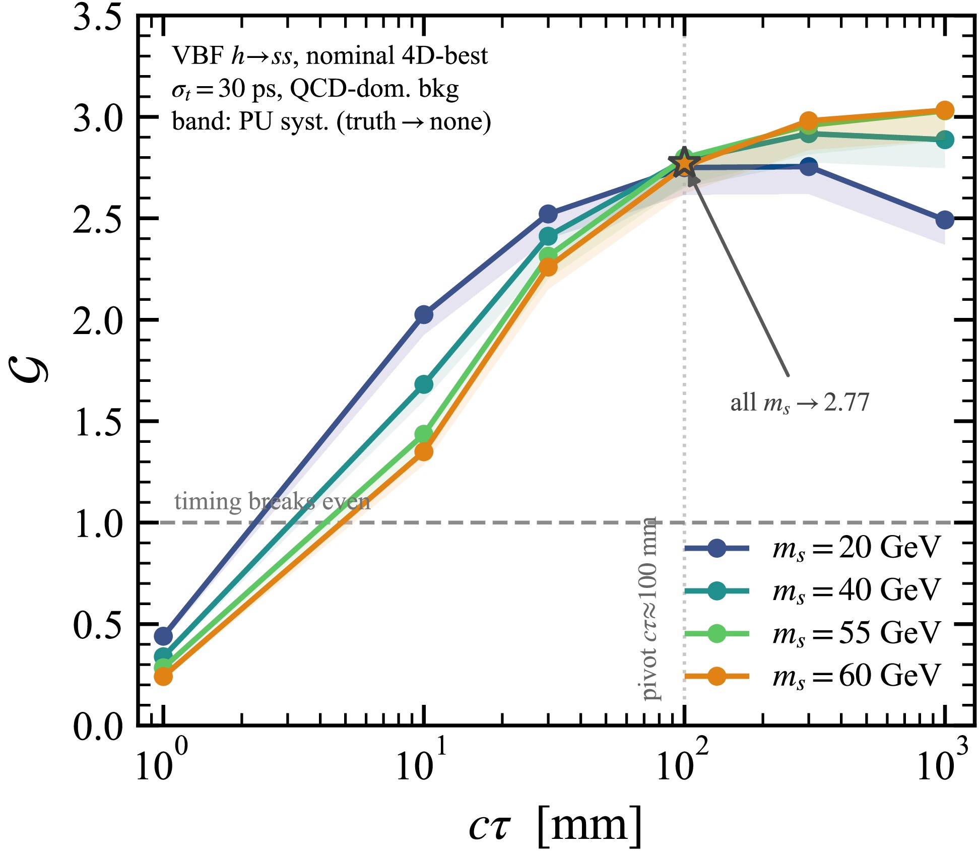
Figure 2. (color online) Normalization-free gain
$ {\cal{G}} $ [Eq. (1)] as a function of decay length for the four scalar masses at the nominal 4D working point ($ \sigma_t=30 \,{\rm{ps}} $ , QCD-dominated background). The dashed line indicates the break-even point,$ {\cal{G}}=1 $ . At$ c\tau\simeq100 \,{\rm{mm}} $ , all masses converge to$ {\cal{G}}\simeq2.8 $ (star), and the mass ordering reverses: lighter scalars yield a larger gain below the pivot, whereas heavier scalars do so above it. Because$ r_B $ is common to all masses, the background normalization cancels in$ {\cal{G}} $ , and the location of the pivot is determined by the signal kinematics alone; threshold and tail-shape systematics are examined separately in the text. -
The timing layer acts almost exclusively on the background (Table A1 in the Supplemental Material): across the grid, it retains
$ r_B=0.073 $ of the spatially selected background at the nominal point and$ r_B=2.1\times10^{-3} $ at the optimized point, while retaining 60%$ \text{–}$ 80% of the signal for$ c\tau\gtrsim30 \,{\rm{mm}} $ . Through Eq. (1), this yields a gain of$ {\cal{G}}=2.8 $ at the nominal working point and$ {\cal{G}}\simeq10 $ at the optimized point for the benchmark$ m_s=60 \;{\rm{GeV}} $ ,$ c\tau=100 \;{\rm{mm}} $ , rising to$ {\cal{G}}\simeq15 $ at$ c\tau=1000 \;{\rm{mm}} $ , where essentially all of the signal is delayed but the prompt background is fully rejected. For$ c\tau\lesssim10 \;{\rm{mm}} $ , the gain falls below unity: the signal delay becomes comparable to$ \sigma_t $ , so the timing cut discards signal without a compensating reduction in background, and the spatial selection alone is preferable.Selection stage Signal QCD $ b\bar bjj $ Generated 200000 2200000 VBF tag jets 53993 369534 $ \geqslant3 $ displaced tracks53884 322922 Displaced vertex ( $ \geqslant3 $ trk,$ R_{{\rm{SV}}}>3 \,{\rm{mm}} $ )39237 122288 $ \displaystyle\sum p_T>10 \,{\rm{GeV}} $ 33583 101500 $ m_{{\rm{SV}}}/\Delta R>4 $ (3D)32145 96435 $ + $ 4D timing (nominal)24276 7021 $ +\ \Delta T_{{\rm{SV}}}>300 \,{\rm{ps}} $ (opt.)14916 200 Table A1. Cutflow for a representative signal benchmark (
$ m_s=55 \,{\rm{GeV}} $ ,$ c\tau=100 \,{\rm{mm}} $ ,$ 2\times10^{5} $ generated events) and the dominant QCD$ b\bar bjj $ background ($ 2.2\times10^{6} $ generated events). The 3D selection terminates at the$ m_{{\rm{SV}}}/\Delta R $ cut; "4D" additionally applies the nominal timing requirement, and "$ \Delta T_{{\rm{SV}}}>300 $ " applies the optimized one. The larger QCD sample sets the statistical precision of the optimized late-time count to$ \simeq$ 7%. The timing layer rejects 93% of the spatially selected QCD vertices and 24% of the signal, consistent with the quantitative content of Eq. (1).The dependence on scalar mass, shown in Fig. 2, is the central structural result. As anticipated from the kinematics—the lab-frame decay length is
$ L_{{\rm{lab}}}\simeq\beta\gamma\, c\tau $ with$ \beta\gamma\simeq p_s/ m_s $ , so the mean boost scales as$ \langle\gamma_s\rangle\propto1/ m_s $ and lighter scalars travel farther for a given proper lifetime— the two mass regimes trade places at a well-defined decay length. At short$ c\tau $ , the larger boost of the light scalar pushes more decays beyond the$ 3 \,{\rm{mm}} $ displacement cut and increases their time delay, so the lighter mass yields the larger gain. At long$ c\tau $ , the same boost carries the light scalar out of the tracker, reducing the signal, and the heavier, slower scalar prevails. The two effects balance at$ c\tau\simeq100 \,{\rm{mm}} $ , where all four masses collapse to$ {\cal{G}}\simeq2.8 $ and the ordering inverts—a crossover that is invisible to a purely spatial analysis, in which the heavier mass is favored at every lifetime, and that emerges only once the temporal dimension is included. This pivot at$ c\tau\simeq 100 \;{\rm{mm}} $ is specific to the assumed tracker fiducial radius and barrel acceptance and would shift for a different detector geometry.
Figure 2. (color online) Normalization-free gain
$ {\cal{G}} $ [Eq. (1)] as a function of decay length for the four scalar masses at the nominal 4D working point ($ \sigma_t=30 \,{\rm{ps}} $ , QCD-dominated background). The dashed line indicates the break-even point,$ {\cal{G}}=1 $ . At$ c\tau\simeq100 \,{\rm{mm}} $ , all masses converge to$ {\cal{G}}\simeq2.8 $ (star), and the mass ordering reverses: lighter scalars yield a larger gain below the pivot, whereas heavier scalars do so above it. Because$ r_B $ is common to all masses, the background normalization cancels in$ {\cal{G}} $ , and the location of the pivot is determined by the signal kinematics alone; threshold and tail-shape systematics are examined separately in the text. -
The timing layer acts almost exclusively on the background (Table A1 in the Supplemental Material): across the grid, it retains
$ r_B=0.073 $ of the spatially selected background at the nominal point and$ r_B=2.1\times10^{-3} $ at the optimized point, while retaining 60%$ \text{–}$ 80% of the signal for$ c\tau\gtrsim30 \,{\rm{mm}} $ . Through Eq. (1), this yields a gain of$ {\cal{G}}=2.8 $ at the nominal working point and$ {\cal{G}}\simeq10 $ at the optimized point for the benchmark$ m_s=60 \;{\rm{GeV}} $ ,$ c\tau=100 \;{\rm{mm}} $ , rising to$ {\cal{G}}\simeq15 $ at$ c\tau=1000 \;{\rm{mm}} $ , where essentially all of the signal is delayed but the prompt background is fully rejected. For$ c\tau\lesssim10 \;{\rm{mm}} $ , the gain falls below unity: the signal delay becomes comparable to$ \sigma_t $ , so the timing cut discards signal without a compensating reduction in background, and the spatial selection alone is preferable.Selection stage Signal QCD $ b\bar bjj $ Generated 200000 2200000 VBF tag jets 53993 369534 $ \geqslant3 $ displaced tracks53884 322922 Displaced vertex ( $ \geqslant3 $ trk,$ R_{{\rm{SV}}}>3 \,{\rm{mm}} $ )39237 122288 $ \displaystyle\sum p_T>10 \,{\rm{GeV}} $ 33583 101500 $ m_{{\rm{SV}}}/\Delta R>4 $ (3D)32145 96435 $ + $ 4D timing (nominal)24276 7021 $ +\ \Delta T_{{\rm{SV}}}>300 \,{\rm{ps}} $ (opt.)14916 200 Table A1. Cutflow for a representative signal benchmark (
$ m_s=55 \,{\rm{GeV}} $ ,$ c\tau=100 \,{\rm{mm}} $ ,$ 2\times10^{5} $ generated events) and the dominant QCD$ b\bar bjj $ background ($ 2.2\times10^{6} $ generated events). The 3D selection terminates at the$ m_{{\rm{SV}}}/\Delta R $ cut; "4D" additionally applies the nominal timing requirement, and "$ \Delta T_{{\rm{SV}}}>300 $ " applies the optimized one. The larger QCD sample sets the statistical precision of the optimized late-time count to$ \simeq$ 7%. The timing layer rejects 93% of the spatially selected QCD vertices and 24% of the signal, consistent with the quantitative content of Eq. (1).The dependence on scalar mass, shown in Fig. 2, is the central structural result. As anticipated from the kinematics—the lab-frame decay length is
$ L_{{\rm{lab}}}\simeq\beta\gamma\, c\tau $ with$ \beta\gamma\simeq p_s/ m_s $ , so the mean boost scales as$ \langle\gamma_s\rangle\propto1/ m_s $ and lighter scalars travel farther for a given proper lifetime— the two mass regimes trade places at a well-defined decay length. At short$ c\tau $ , the larger boost of the light scalar pushes more decays beyond the$ 3 \,{\rm{mm}} $ displacement cut and increases their time delay, so the lighter mass yields the larger gain. At long$ c\tau $ , the same boost carries the light scalar out of the tracker, reducing the signal, and the heavier, slower scalar prevails. The two effects balance at$ c\tau\simeq100 \,{\rm{mm}} $ , where all four masses collapse to$ {\cal{G}}\simeq2.8 $ and the ordering inverts—a crossover that is invisible to a purely spatial analysis, in which the heavier mass is favored at every lifetime, and that emerges only once the temporal dimension is included. This pivot at$ c\tau\simeq 100 \;{\rm{mm}} $ is specific to the assumed tracker fiducial radius and barrel acceptance and would shift for a different detector geometry.
Figure 2. (color online) Normalization-free gain
$ {\cal{G}} $ [Eq. (1)] as a function of decay length for the four scalar masses at the nominal 4D working point ($ \sigma_t=30 \,{\rm{ps}} $ , QCD-dominated background). The dashed line indicates the break-even point,$ {\cal{G}}=1 $ . At$ c\tau\simeq100 \,{\rm{mm}} $ , all masses converge to$ {\cal{G}}\simeq2.8 $ (star), and the mass ordering reverses: lighter scalars yield a larger gain below the pivot, whereas heavier scalars do so above it. Because$ r_B $ is common to all masses, the background normalization cancels in$ {\cal{G}} $ , and the location of the pivot is determined by the signal kinematics alone; threshold and tail-shape systematics are examined separately in the text. -
To place the gain in physical context, we translate the selection into an illustrative, statistics-limited 95% CL upper limit on
$ {\rm{BR}}(h\to ss) $ at$ {\cal{L}}=3000 \;{\rm{fb}}^{-1} $ (again assuming$ {\rm{BR}}(s\to b\bar b)=1 $ ), using the asymptotic$ {\rm{CL}}_s $ procedure [38, 39] for a single-bin counting experiment; the signal strength scales linearly with the branching ratio. These limits are an idealized floor: the absolute background normalization is not predicted by the fast simulation and must be supplied by a data-driven estimate in a real experiment, an effect that we bracket below through$ \kappa_b $ . Figure A4 in the Supplemental Material shows the expected limit for$ m_s=60 \;{\rm{GeV}} $ . Adding timing tightens the floor from$ {\rm{BR}}\simeq0.19 $ (3D) to$ \simeq0.019 $ (optimized 4D) at$ c\tau=100 \;{\rm{mm}} $ , with the improvement tracking the gain of Fig. 2; the best reach across the plane,$ {\rm{BR}}\simeq0.019 $ , is obtained for$ m_s=55\text{–}60 \;{\rm{GeV}} $ at$ c\tau=100 \;{\rm{mm}} $ . The upper point,$ m_s=60 \;{\rm{GeV}} $ , lies close to the$ m_s\to m_h/2 $ kinematic threshold, where the narrow phase space makes the decay kinematics more sensitive to off-shell and generator effects, so we treat it as a near-threshold benchmark rather than a sharp optimum.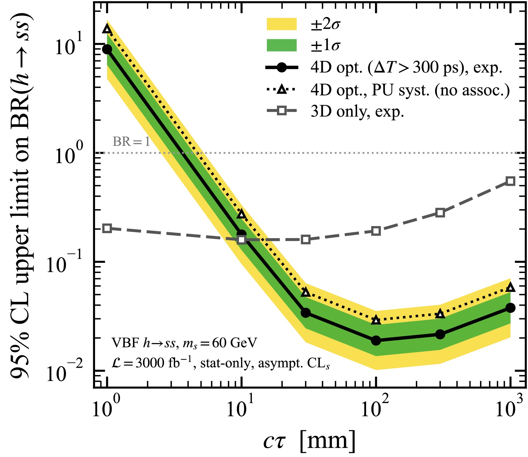
Figure A4. (color online) Illustrative, statistics-limited 95% CL upper limit on
$ {\rm{BR}}(h\to ss) $ , assuming$ {\rm{BR}}(s\to b\bar b)=1 $ (equivalently, a limit on$ {\rm{BR}}(h\to ss)\,[{\rm{BR}}(s\to b\bar b)]^2 $ ), as a function of decay length for$ m_s=60 \,{\rm{GeV}} $ at$ 3000 \,{\rm{fb}}^{-1} $ , for the optimized 4D selection (solid, with$ \pm1,2\sigma $ bands), the same selection under the conservative no-association pileup systematic (dotted), and the 3D-only selection (dashed). Only statistical uncertainties are shown on the central curves; the absolute reach is an idealized floor set by the background normalization (see text). The separation between the solid and dotted curves brackets the pileup-association uncertainty. The timing layer improves the limit for$ c\tau\gtrsim20 \,{\rm{mm}} $ and is counterproductive for the most prompt decays.The complementarity to existing searches is sharpest at long lifetimes. The spatial search of Ref. [10] is most sensitive around
$ c\tau\simeq5\text{–}70 \;{\rm{mm}} $ and loses reach beyond$ \sim100 \;{\rm{mm}} $ , as decays increasingly fall outside the tracker fiducial volume and prompt-background rejection no longer improves. By contrast, the timing gain grows with$ c\tau $ , since the exploited delay scales with the flight distance. Although the in-tracker signal acceptance falls for both approaches, the 4D limit degrades far more gently and remains at$ {\rm{BR}}\simeq0.02\text{–}0.04 $ out to$ c\tau=1000 \;{\rm{mm}} $ , the regime in which a purely spatial limit has risen above the physical$ {\rm{BR}}=1 $ boundary. Timing therefore extends the reach into the long-lifetime region that a spatial-only selection cannot cover. -
To place the gain in physical context, we translate the selection into an illustrative, statistics-limited 95% CL upper limit on
$ {\rm{BR}}(h\to ss) $ at$ {\cal{L}}=3000 \;{\rm{fb}}^{-1} $ (again assuming$ {\rm{BR}}(s\to b\bar b)=1 $ ), using the asymptotic$ {\rm{CL}}_s $ procedure [38, 39] for a single-bin counting experiment; the signal strength scales linearly with the branching ratio. These limits are an idealized floor: the absolute background normalization is not predicted by the fast simulation and must be supplied by a data-driven estimate in a real experiment, an effect that we bracket below through$ \kappa_b $ . Figure A4 in the Supplemental Material shows the expected limit for$ m_s=60 \;{\rm{GeV}} $ . Adding timing tightens the floor from$ {\rm{BR}}\simeq0.19 $ (3D) to$ \simeq0.019 $ (optimized 4D) at$ c\tau=100 \;{\rm{mm}} $ , with the improvement tracking the gain of Fig. 2; the best reach across the plane,$ {\rm{BR}}\simeq0.019 $ , is obtained for$ m_s=55\text{–}60 \;{\rm{GeV}} $ at$ c\tau=100 \;{\rm{mm}} $ . The upper point,$ m_s=60 \;{\rm{GeV}} $ , lies close to the$ m_s\to m_h/2 $ kinematic threshold, where the narrow phase space makes the decay kinematics more sensitive to off-shell and generator effects, so we treat it as a near-threshold benchmark rather than a sharp optimum.
Figure A4. (color online) Illustrative, statistics-limited 95% CL upper limit on
$ {\rm{BR}}(h\to ss) $ , assuming$ {\rm{BR}}(s\to b\bar b)=1 $ (equivalently, a limit on$ {\rm{BR}}(h\to ss)\,[{\rm{BR}}(s\to b\bar b)]^2 $ ), as a function of decay length for$ m_s=60 \,{\rm{GeV}} $ at$ 3000 \,{\rm{fb}}^{-1} $ , for the optimized 4D selection (solid, with$ \pm1,2\sigma $ bands), the same selection under the conservative no-association pileup systematic (dotted), and the 3D-only selection (dashed). Only statistical uncertainties are shown on the central curves; the absolute reach is an idealized floor set by the background normalization (see text). The separation between the solid and dotted curves brackets the pileup-association uncertainty. The timing layer improves the limit for$ c\tau\gtrsim20 \,{\rm{mm}} $ and is counterproductive for the most prompt decays.The complementarity to existing searches is sharpest at long lifetimes. The spatial search of Ref. [10] is most sensitive around
$ c\tau\simeq5\text{–}70 \;{\rm{mm}} $ and loses reach beyond$ \sim100 \;{\rm{mm}} $ , as decays increasingly fall outside the tracker fiducial volume and prompt-background rejection no longer improves. By contrast, the timing gain grows with$ c\tau $ , since the exploited delay scales with the flight distance. Although the in-tracker signal acceptance falls for both approaches, the 4D limit degrades far more gently and remains at$ {\rm{BR}}\simeq0.02\text{–}0.04 $ out to$ c\tau=1000 \;{\rm{mm}} $ , the regime in which a purely spatial limit has risen above the physical$ {\rm{BR}}=1 $ boundary. Timing therefore extends the reach into the long-lifetime region that a spatial-only selection cannot cover. -
To place the gain in physical context, we translate the selection into an illustrative, statistics-limited 95% CL upper limit on
$ {\rm{BR}}(h\to ss) $ at$ {\cal{L}}=3000 \;{\rm{fb}}^{-1} $ (again assuming$ {\rm{BR}}(s\to b\bar b)=1 $ ), using the asymptotic$ {\rm{CL}}_s $ procedure [38, 39] for a single-bin counting experiment; the signal strength scales linearly with the branching ratio. These limits are an idealized floor: the absolute background normalization is not predicted by the fast simulation and must be supplied by a data-driven estimate in a real experiment, an effect that we bracket below through$ \kappa_b $ . Figure A4 in the Supplemental Material shows the expected limit for$ m_s=60 \;{\rm{GeV}} $ . Adding timing tightens the floor from$ {\rm{BR}}\simeq0.19 $ (3D) to$ \simeq0.019 $ (optimized 4D) at$ c\tau=100 \;{\rm{mm}} $ , with the improvement tracking the gain of Fig. 2; the best reach across the plane,$ {\rm{BR}}\simeq0.019 $ , is obtained for$ m_s=55\text{–}60 \;{\rm{GeV}} $ at$ c\tau=100 \;{\rm{mm}} $ . The upper point,$ m_s=60 \;{\rm{GeV}} $ , lies close to the$ m_s\to m_h/2 $ kinematic threshold, where the narrow phase space makes the decay kinematics more sensitive to off-shell and generator effects, so we treat it as a near-threshold benchmark rather than a sharp optimum.
Figure A4. (color online) Illustrative, statistics-limited 95% CL upper limit on
$ {\rm{BR}}(h\to ss) $ , assuming$ {\rm{BR}}(s\to b\bar b)=1 $ (equivalently, a limit on$ {\rm{BR}}(h\to ss)\,[{\rm{BR}}(s\to b\bar b)]^2 $ ), as a function of decay length for$ m_s=60 \,{\rm{GeV}} $ at$ 3000 \,{\rm{fb}}^{-1} $ , for the optimized 4D selection (solid, with$ \pm1,2\sigma $ bands), the same selection under the conservative no-association pileup systematic (dotted), and the 3D-only selection (dashed). Only statistical uncertainties are shown on the central curves; the absolute reach is an idealized floor set by the background normalization (see text). The separation between the solid and dotted curves brackets the pileup-association uncertainty. The timing layer improves the limit for$ c\tau\gtrsim20 \,{\rm{mm}} $ and is counterproductive for the most prompt decays.The complementarity to existing searches is sharpest at long lifetimes. The spatial search of Ref. [10] is most sensitive around
$ c\tau\simeq5\text{–}70 \;{\rm{mm}} $ and loses reach beyond$ \sim100 \;{\rm{mm}} $ , as decays increasingly fall outside the tracker fiducial volume and prompt-background rejection no longer improves. By contrast, the timing gain grows with$ c\tau $ , since the exploited delay scales with the flight distance. Although the in-tracker signal acceptance falls for both approaches, the 4D limit degrades far more gently and remains at$ {\rm{BR}}\simeq0.02\text{–}0.04 $ out to$ c\tau=1000 \;{\rm{mm}} $ , the regime in which a purely spatial limit has risen above the physical$ {\rm{BR}}=1 $ boundary. Timing therefore extends the reach into the long-lifetime region that a spatial-only selection cannot cover. -
Four effects bound the projection, and Table 1 summarizes the stability of the gain
$ {\cal{G}} $ at the benchmark against the principal detector and selection nuisances. Pileup. The signal is robust against how pileup (pu) tracks are removed: switching from the truth-association proxy (pu=truth) to no removal at all (pu=none) shifts the signal yield and vertex-matching purity by$ \lesssim$ 3%, because a displaced vertex is a coherent object—several tracks sharing a common late time and a common displaced position—that random pileup cannot mimic. The background is not. With pileup tracks left in, the$ \pm180 \,{\rm{ps}} $ pileup time spread is attached to the prompt QCD vertices and smears them into the late tail, raising the background timing survival by$ \simeq$ 10% at the nominal point and more than doubling it (a factor of$ \simeq2.4 $ ) at the optimized one in this no-association extreme. This brackets the gain between its ideal-association value and a conservative no-association value, degrading$ {\cal{G}} $ by$ \lesssim$ 5% (nominal) and$ \lesssim$ 35% (optimized). These figures are evaluated directly for the barrel timing layer (QCD re-simulated with no pileup-track association,$ 2.2\times10^{6} $ events), rather than transferred from a different timing geometry. The realistic case lies between the two and close to the ideal, because the experiment associates tracks to vertices by time and position: a per-track time veto cannot be used to remove pileup here, since it would also discard the genuinely late signal. Separating coherent late signal from random late pileup is therefore intrinsically a vertex-level rather than a track-level operation. Crucially,$ r_B $ is common to every signal point, so the mass-trend reversal of Fig. 2 remains intact under this uncertainty. Start time. Degrading$ t_0 $ from its idealized$ \simeq8 \;{\rm{ps}} $ to a realistic$ 30 \;{\rm{ps}} $ leaves the long-lifetime gain unchanged, because the signal delay there ($ \Delta T_{{\rm{SV}}}\gtrsim400 \;{\rm{ps}} $ ) far exceeds$ \sigma_{t_0} $ . Even in the short-lifetime region, the effect is modest: the broader start time smears the prompt background by the same amount, raising the nominal background survival by$ \simeq$ 16% and lowering the nominal-point gain by$ \lesssim$ 7% for$ c\tau=10 $ –$ 30 \;{\rm{mm}} $ , while shifting the break-even point by$ \lesssim0.3 \;{\rm{mm}} $ . The optimized$ \Delta T_{{\rm{SV}}}>300 \;{\rm{ps}} $ working point is essentially immune ($ \lesssim$ 2% change in background survival), since a$ 30 \,{\rm{ps}} $ resolution cannot promote a prompt vertex beyond a$ 300 \;{\rm{ps}} $ threshold. Tail statistics. The optimized$ \Delta T_{{\rm{SV}}}>300 \;{\rm{ps}} $ working point retains$ \simeq200 $ QCD vertices out of the$ 2.2\times10^{6} $ -event sample, corresponding to a$ \simeq$ 7% Monte Carlo statistical uncertainty on$ r_B $ that propagates directly to the optimized gain and to the corresponding limit. The shape of the prompt late-time tail beyond the simulated statistics is not predicted by a fast simulation and would, in a real analysis, be constrained by a sideband fit to the$ \Delta T_{{\rm{SV}}} $ distribution. We therefore quote this working point as an illustrative tighter selection rather than a fully exploited optimum. Background normalization. As a phenomenological projection, this study has no data with which to normalize the QCD continuum, which yields$ {\cal{O}}(10^{6}\text{–}10^{8}) $ selected events at$ 3000 \;{\rm{fb}}^{-1} $ ; a fractional background uncertainty of even$ \kappa_b\sim$ 1% would then exceed the statistical error by one to two orders of magnitude. The absolute limits are therefore a statistics-limited floor, and we present them as a function of an assumed$ \kappa_b $ that brackets what a data-driven control-region estimate would achieve in a real experiment. This systematics-dominated regime in fact strengthens the case for timing: because the optimized selection reduces the background by a further factor of$ \simeq500 $ , the 4D limit is far less sensitive to$ \kappa_b $ than the 3D one. At$ \kappa_b=$ 1%, the spatial search no longer excludes any physically allowed branching ratio, with its limit lying above unity over the entire lifetime range, whereas the optimized 4D search still excludes$ {\rm{BR}}\lesssim0.1 $ for$ c\tau\gtrsim 10 \;{\rm{mm}} $ —a median limit lower by a factor of$ \simeq216 $ at the benchmark$ c\tau=100 \;{\rm{mm}} $ (Fig. A5 in the Supplemental Material). The advantage of timing over a purely spatial search therefore grows as the background uncertainty increases. Moreover, a fast simulation does not capture the degradation of displaced-track efficiency and impact-parameter resolution with displacement, nor displaced-track fakes. These act on the spatially selected vertices that enter the numerator and denominator of both$ r_S $ and$ r_B $ in a correlated way and therefore largely cancel in the ratio$ {\cal{G}} $ , but they would have to be calibrated from data or with a full simulation before the absolute limits could be regarded as experiment-grade. None of these effects affects the normalization-free gain$ {\cal{G}} $ .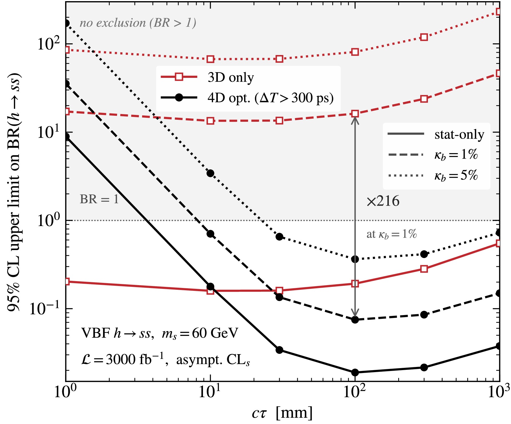
Figure A5. (color online) Expected 95% CL upper limits on
$ {\rm{BR}}(h\to ss) $ (assuming$ {\rm{BR}}(s\to b\bar b)=1 $ ) as a function of decay length for$ m_s=60 \;{\rm{GeV}} $ at$ 3000 \;{\rm{fb}}^{-1} $ , for the 3D-only (red) and optimized-4D (black) selections, each shown for an assumed background-normalization uncertainty$ \kappa_b=0 $ (solid), 1% (dashed), and 5% (dotted). The shaded band denotes the unphysical region$ {\rm{BR}}>1 $ , in which an upper limit excludes no allowed branching ratio. For$ \kappa_b\geqslant$ 1%, the entire 3D curve lies in this region, whereas the optimized-4D curve remains below the$ {\rm{BR}}=1 $ boundary. The arrow indicates the factor$ \simeq216 $ separating the two selections at the benchmark$ c\tau= $ $ 100 \;{\rm{mm}} $ for$ \kappa_b=$ 1%. Statistical bands are omitted for clarity. -
Four effects bound the projection, and Table 1 summarizes the stability of the gain
$ {\cal{G}} $ at the benchmark against the principal detector and selection nuisances. Pileup. The signal is robust against how pileup (pu) tracks are removed: switching from the truth-association proxy (pu=truth) to no removal at all (pu=none) shifts the signal yield and vertex-matching purity by$ \lesssim$ 3%, because a displaced vertex is a coherent object—several tracks sharing a common late time and a common displaced position—that random pileup cannot mimic. The background is not. With pileup tracks left in, the$ \pm180 \,{\rm{ps}} $ pileup time spread is attached to the prompt QCD vertices and smears them into the late tail, raising the background timing survival by$ \simeq$ 10% at the nominal point and more than doubling it (a factor of$ \simeq2.4 $ ) at the optimized one in this no-association extreme. This brackets the gain between its ideal-association value and a conservative no-association value, degrading$ {\cal{G}} $ by$ \lesssim$ 5% (nominal) and$ \lesssim$ 35% (optimized). These figures are evaluated directly for the barrel timing layer (QCD re-simulated with no pileup-track association,$ 2.2\times10^{6} $ events), rather than transferred from a different timing geometry. The realistic case lies between the two and close to the ideal, because the experiment associates tracks to vertices by time and position: a per-track time veto cannot be used to remove pileup here, since it would also discard the genuinely late signal. Separating coherent late signal from random late pileup is therefore intrinsically a vertex-level rather than a track-level operation. Crucially,$ r_B $ is common to every signal point, so the mass-trend reversal of Fig. 2 remains intact under this uncertainty. Start time. Degrading$ t_0 $ from its idealized$ \simeq8 \;{\rm{ps}} $ to a realistic$ 30 \;{\rm{ps}} $ leaves the long-lifetime gain unchanged, because the signal delay there ($ \Delta T_{{\rm{SV}}}\gtrsim400 \;{\rm{ps}} $ ) far exceeds$ \sigma_{t_0} $ . Even in the short-lifetime region, the effect is modest: the broader start time smears the prompt background by the same amount, raising the nominal background survival by$ \simeq$ 16% and lowering the nominal-point gain by$ \lesssim$ 7% for$ c\tau=10 $ –$ 30 \;{\rm{mm}} $ , while shifting the break-even point by$ \lesssim0.3 \;{\rm{mm}} $ . The optimized$ \Delta T_{{\rm{SV}}}>300 \;{\rm{ps}} $ working point is essentially immune ($ \lesssim$ 2% change in background survival), since a$ 30 \,{\rm{ps}} $ resolution cannot promote a prompt vertex beyond a$ 300 \;{\rm{ps}} $ threshold. Tail statistics. The optimized$ \Delta T_{{\rm{SV}}}>300 \;{\rm{ps}} $ working point retains$ \simeq200 $ QCD vertices out of the$ 2.2\times10^{6} $ -event sample, corresponding to a$ \simeq$ 7% Monte Carlo statistical uncertainty on$ r_B $ that propagates directly to the optimized gain and to the corresponding limit. The shape of the prompt late-time tail beyond the simulated statistics is not predicted by a fast simulation and would, in a real analysis, be constrained by a sideband fit to the$ \Delta T_{{\rm{SV}}} $ distribution. We therefore quote this working point as an illustrative tighter selection rather than a fully exploited optimum. Background normalization. As a phenomenological projection, this study has no data with which to normalize the QCD continuum, which yields$ {\cal{O}}(10^{6}\text{–}10^{8}) $ selected events at$ 3000 \;{\rm{fb}}^{-1} $ ; a fractional background uncertainty of even$ \kappa_b\sim$ 1% would then exceed the statistical error by one to two orders of magnitude. The absolute limits are therefore a statistics-limited floor, and we present them as a function of an assumed$ \kappa_b $ that brackets what a data-driven control-region estimate would achieve in a real experiment. This systematics-dominated regime in fact strengthens the case for timing: because the optimized selection reduces the background by a further factor of$ \simeq500 $ , the 4D limit is far less sensitive to$ \kappa_b $ than the 3D one. At$ \kappa_b=$ 1%, the spatial search no longer excludes any physically allowed branching ratio, with its limit lying above unity over the entire lifetime range, whereas the optimized 4D search still excludes$ {\rm{BR}}\lesssim0.1 $ for$ c\tau\gtrsim 10 \;{\rm{mm}} $ —a median limit lower by a factor of$ \simeq216 $ at the benchmark$ c\tau=100 \;{\rm{mm}} $ (Fig. A5 in the Supplemental Material). The advantage of timing over a purely spatial search therefore grows as the background uncertainty increases. Moreover, a fast simulation does not capture the degradation of displaced-track efficiency and impact-parameter resolution with displacement, nor displaced-track fakes. These act on the spatially selected vertices that enter the numerator and denominator of both$ r_S $ and$ r_B $ in a correlated way and therefore largely cancel in the ratio$ {\cal{G}} $ , but they would have to be calibrated from data or with a full simulation before the absolute limits could be regarded as experiment-grade. None of these effects affects the normalization-free gain$ {\cal{G}} $ .
Figure A5. (color online) Expected 95% CL upper limits on
$ {\rm{BR}}(h\to ss) $ (assuming$ {\rm{BR}}(s\to b\bar b)=1 $ ) as a function of decay length for$ m_s=60 \;{\rm{GeV}} $ at$ 3000 \;{\rm{fb}}^{-1} $ , for the 3D-only (red) and optimized-4D (black) selections, each shown for an assumed background-normalization uncertainty$ \kappa_b=0 $ (solid), 1% (dashed), and 5% (dotted). The shaded band denotes the unphysical region$ {\rm{BR}}>1 $ , in which an upper limit excludes no allowed branching ratio. For$ \kappa_b\geqslant$ 1%, the entire 3D curve lies in this region, whereas the optimized-4D curve remains below the$ {\rm{BR}}=1 $ boundary. The arrow indicates the factor$ \simeq216 $ separating the two selections at the benchmark$ c\tau= $ $ 100 \;{\rm{mm}} $ for$ \kappa_b=$ 1%. Statistical bands are omitted for clarity. -
Four effects bound the projection, and Table 1 summarizes the stability of the gain
$ {\cal{G}} $ at the benchmark against the principal detector and selection nuisances. Pileup. The signal is robust against how pileup (pu) tracks are removed: switching from the truth-association proxy (pu=truth) to no removal at all (pu=none) shifts the signal yield and vertex-matching purity by$ \lesssim$ 3%, because a displaced vertex is a coherent object—several tracks sharing a common late time and a common displaced position—that random pileup cannot mimic. The background is not. With pileup tracks left in, the$ \pm180 \,{\rm{ps}} $ pileup time spread is attached to the prompt QCD vertices and smears them into the late tail, raising the background timing survival by$ \simeq$ 10% at the nominal point and more than doubling it (a factor of$ \simeq2.4 $ ) at the optimized one in this no-association extreme. This brackets the gain between its ideal-association value and a conservative no-association value, degrading$ {\cal{G}} $ by$ \lesssim$ 5% (nominal) and$ \lesssim$ 35% (optimized). These figures are evaluated directly for the barrel timing layer (QCD re-simulated with no pileup-track association,$ 2.2\times10^{6} $ events), rather than transferred from a different timing geometry. The realistic case lies between the two and close to the ideal, because the experiment associates tracks to vertices by time and position: a per-track time veto cannot be used to remove pileup here, since it would also discard the genuinely late signal. Separating coherent late signal from random late pileup is therefore intrinsically a vertex-level rather than a track-level operation. Crucially,$ r_B $ is common to every signal point, so the mass-trend reversal of Fig. 2 remains intact under this uncertainty. Start time. Degrading$ t_0 $ from its idealized$ \simeq8 \;{\rm{ps}} $ to a realistic$ 30 \;{\rm{ps}} $ leaves the long-lifetime gain unchanged, because the signal delay there ($ \Delta T_{{\rm{SV}}}\gtrsim400 \;{\rm{ps}} $ ) far exceeds$ \sigma_{t_0} $ . Even in the short-lifetime region, the effect is modest: the broader start time smears the prompt background by the same amount, raising the nominal background survival by$ \simeq$ 16% and lowering the nominal-point gain by$ \lesssim$ 7% for$ c\tau=10 $ –$ 30 \;{\rm{mm}} $ , while shifting the break-even point by$ \lesssim0.3 \;{\rm{mm}} $ . The optimized$ \Delta T_{{\rm{SV}}}>300 \;{\rm{ps}} $ working point is essentially immune ($ \lesssim$ 2% change in background survival), since a$ 30 \,{\rm{ps}} $ resolution cannot promote a prompt vertex beyond a$ 300 \;{\rm{ps}} $ threshold. Tail statistics. The optimized$ \Delta T_{{\rm{SV}}}>300 \;{\rm{ps}} $ working point retains$ \simeq200 $ QCD vertices out of the$ 2.2\times10^{6} $ -event sample, corresponding to a$ \simeq$ 7% Monte Carlo statistical uncertainty on$ r_B $ that propagates directly to the optimized gain and to the corresponding limit. The shape of the prompt late-time tail beyond the simulated statistics is not predicted by a fast simulation and would, in a real analysis, be constrained by a sideband fit to the$ \Delta T_{{\rm{SV}}} $ distribution. We therefore quote this working point as an illustrative tighter selection rather than a fully exploited optimum. Background normalization. As a phenomenological projection, this study has no data with which to normalize the QCD continuum, which yields$ {\cal{O}}(10^{6}\text{–}10^{8}) $ selected events at$ 3000 \;{\rm{fb}}^{-1} $ ; a fractional background uncertainty of even$ \kappa_b\sim$ 1% would then exceed the statistical error by one to two orders of magnitude. The absolute limits are therefore a statistics-limited floor, and we present them as a function of an assumed$ \kappa_b $ that brackets what a data-driven control-region estimate would achieve in a real experiment. This systematics-dominated regime in fact strengthens the case for timing: because the optimized selection reduces the background by a further factor of$ \simeq500 $ , the 4D limit is far less sensitive to$ \kappa_b $ than the 3D one. At$ \kappa_b=$ 1%, the spatial search no longer excludes any physically allowed branching ratio, with its limit lying above unity over the entire lifetime range, whereas the optimized 4D search still excludes$ {\rm{BR}}\lesssim0.1 $ for$ c\tau\gtrsim 10 \;{\rm{mm}} $ —a median limit lower by a factor of$ \simeq216 $ at the benchmark$ c\tau=100 \;{\rm{mm}} $ (Fig. A5 in the Supplemental Material). The advantage of timing over a purely spatial search therefore grows as the background uncertainty increases. Moreover, a fast simulation does not capture the degradation of displaced-track efficiency and impact-parameter resolution with displacement, nor displaced-track fakes. These act on the spatially selected vertices that enter the numerator and denominator of both$ r_S $ and$ r_B $ in a correlated way and therefore largely cancel in the ratio$ {\cal{G}} $ , but they would have to be calibrated from data or with a full simulation before the absolute limits could be regarded as experiment-grade. None of these effects affects the normalization-free gain$ {\cal{G}} $ .
Figure A5. (color online) Expected 95% CL upper limits on
$ {\rm{BR}}(h\to ss) $ (assuming$ {\rm{BR}}(s\to b\bar b)=1 $ ) as a function of decay length for$ m_s=60 \;{\rm{GeV}} $ at$ 3000 \;{\rm{fb}}^{-1} $ , for the 3D-only (red) and optimized-4D (black) selections, each shown for an assumed background-normalization uncertainty$ \kappa_b=0 $ (solid), 1% (dashed), and 5% (dotted). The shaded band denotes the unphysical region$ {\rm{BR}}>1 $ , in which an upper limit excludes no allowed branching ratio. For$ \kappa_b\geqslant$ 1%, the entire 3D curve lies in this region, whereas the optimized-4D curve remains below the$ {\rm{BR}}=1 $ boundary. The arrow indicates the factor$ \simeq216 $ separating the two selections at the benchmark$ c\tau= $ $ 100 \;{\rm{mm}} $ for$ \kappa_b=$ 1%. Statistical bands are omitted for clarity. -
We have shown that the forward tag jets of vector-boson fusion identify a hard-scatter vertex whose prompt central tracks, timed by a barrel timing layer, supply a clean event-by-event start time that converts a displaced vertex into a four-dimensional object, and that the resulting timing layer acts almost exclusively on the prompt heavy-flavor background that no spatial cut can remove. The mechanism is internally consistent: the same forward, high-mass dijet that defines the VBF signal region also tags the vertex furnishing the timing reference, so the temporal handle comes for free with the spatial one.
Quantitatively, timing improves the sensitivity by a normalization-free factor
$ {\cal{G}}=2.8 $ at the nominal working point and by up to an order of magnitude for a tighter delayed-vertex requirement. Under the explicit assumption$ {\rm{BR}}(s\to b\bar b)=1 $ , this corresponds to an illustrative, statistics-limited$ {\rm{BR}}(h\to ss) $ floor that can approach$ \simeq$ 2% for$ m_s=55\text{–}60 \,{\rm{GeV}} $ at intermediate lifetimes. Without the timing dimension, separating a genuine long-lived decay from the prompt heavy-flavor continuum requires a spatial displacement large enough to overcome that continuum's sub-millimeter tail; with timing included, the same separation is achieved through a time delay that the background cannot produce, and the two requirements are independent. The structural signature of this independence is the mass-trend reversal at$ c\tau\simeq100 \,{\rm{mm}} $ , where the boost-driven and containment-driven mass dependences cancel.These projections are complementary to recent spatial searches [10–12], one of which already constrains this VBF topology with Run-2 data but is purely spatial and, in its VBF region, systematics-limited. At the HL-LHC, additional luminosity alone cannot improve a background-systematics-limited spatial search; the timing layer reduces the surviving background by a further factor of
$ \simeq500 $ , substantially reducing the dependence on the background normalization, and its advantage is largest precisely at long lifetimes,$ c\tau\gtrsim100 \,{\rm{mm}} $ , where the spatial handle weakens. Timing is thus the lever that keeps this search class improving where luminosity and spatial information alone have saturated.What remains is specific to an experimental realization rather than to the method: a data-driven control-region estimate of the QCD continuum, which only collision data can provide and whose impact we have bracketed through
$ \kappa_b $ , and a dedicated mapping of the start-time and pileup systematics across the short-lifetime region for the barrel-only timing configuration. Neither affects the gain$ {\cal{G}} $ , which we therefore advance as the primary, detector-robust result. -
We have shown that the forward tag jets of vector-boson fusion identify a hard-scatter vertex whose prompt central tracks, timed by a barrel timing layer, supply a clean event-by-event start time that converts a displaced vertex into a four-dimensional object, and that the resulting timing layer acts almost exclusively on the prompt heavy-flavor background that no spatial cut can remove. The mechanism is internally consistent: the same forward, high-mass dijet that defines the VBF signal region also tags the vertex furnishing the timing reference, so the temporal handle comes for free with the spatial one.
Quantitatively, timing improves the sensitivity by a normalization-free factor
$ {\cal{G}}=2.8 $ at the nominal working point and by up to an order of magnitude for a tighter delayed-vertex requirement. Under the explicit assumption$ {\rm{BR}}(s\to b\bar b)=1 $ , this corresponds to an illustrative, statistics-limited$ {\rm{BR}}(h\to ss) $ floor that can approach$ \simeq$ 2% for$ m_s=55\text{–}60 \,{\rm{GeV}} $ at intermediate lifetimes. Without the timing dimension, separating a genuine long-lived decay from the prompt heavy-flavor continuum requires a spatial displacement large enough to overcome that continuum's sub-millimeter tail; with timing included, the same separation is achieved through a time delay that the background cannot produce, and the two requirements are independent. The structural signature of this independence is the mass-trend reversal at$ c\tau\simeq100 \,{\rm{mm}} $ , where the boost-driven and containment-driven mass dependences cancel.These projections are complementary to recent spatial searches [10–12], one of which already constrains this VBF topology with Run-2 data but is purely spatial and, in its VBF region, systematics-limited. At the HL-LHC, additional luminosity alone cannot improve a background-systematics-limited spatial search; the timing layer reduces the surviving background by a further factor of
$ \simeq500 $ , substantially reducing the dependence on the background normalization, and its advantage is largest precisely at long lifetimes,$ c\tau\gtrsim100 \,{\rm{mm}} $ , where the spatial handle weakens. Timing is thus the lever that keeps this search class improving where luminosity and spatial information alone have saturated.What remains is specific to an experimental realization rather than to the method: a data-driven control-region estimate of the QCD continuum, which only collision data can provide and whose impact we have bracketed through
$ \kappa_b $ , and a dedicated mapping of the start-time and pileup systematics across the short-lifetime region for the barrel-only timing configuration. Neither affects the gain$ {\cal{G}} $ , which we therefore advance as the primary, detector-robust result. -
We have shown that the forward tag jets of vector-boson fusion identify a hard-scatter vertex whose prompt central tracks, timed by a barrel timing layer, supply a clean event-by-event start time that converts a displaced vertex into a four-dimensional object, and that the resulting timing layer acts almost exclusively on the prompt heavy-flavor background that no spatial cut can remove. The mechanism is internally consistent: the same forward, high-mass dijet that defines the VBF signal region also tags the vertex furnishing the timing reference, so the temporal handle comes for free with the spatial one.
Quantitatively, timing improves the sensitivity by a normalization-free factor
$ {\cal{G}}=2.8 $ at the nominal working point and by up to an order of magnitude for a tighter delayed-vertex requirement. Under the explicit assumption$ {\rm{BR}}(s\to b\bar b)=1 $ , this corresponds to an illustrative, statistics-limited$ {\rm{BR}}(h\to ss) $ floor that can approach$ \simeq$ 2% for$ m_s=55\text{–}60 \,{\rm{GeV}} $ at intermediate lifetimes. Without the timing dimension, separating a genuine long-lived decay from the prompt heavy-flavor continuum requires a spatial displacement large enough to overcome that continuum's sub-millimeter tail; with timing included, the same separation is achieved through a time delay that the background cannot produce, and the two requirements are independent. The structural signature of this independence is the mass-trend reversal at$ c\tau\simeq100 \,{\rm{mm}} $ , where the boost-driven and containment-driven mass dependences cancel.These projections are complementary to recent spatial searches [10–12], one of which already constrains this VBF topology with Run-2 data but is purely spatial and, in its VBF region, systematics-limited. At the HL-LHC, additional luminosity alone cannot improve a background-systematics-limited spatial search; the timing layer reduces the surviving background by a further factor of
$ \simeq500 $ , substantially reducing the dependence on the background normalization, and its advantage is largest precisely at long lifetimes,$ c\tau\gtrsim100 \,{\rm{mm}} $ , where the spatial handle weakens. Timing is thus the lever that keeps this search class improving where luminosity and spatial information alone have saturated.What remains is specific to an experimental realization rather than to the method: a data-driven control-region estimate of the QCD continuum, which only collision data can provide and whose impact we have bracketed through
$ \kappa_b $ , and a dedicated mapping of the start-time and pileup systematics across the short-lifetime region for the barrel-only timing configuration. Neither affects the gain$ {\cal{G}} $ , which we therefore advance as the primary, detector-robust result. -
The author thanks colleagues at the Institute of High Energy Physics for stimulating discussions.
-
The author thanks colleagues at the Institute of High Energy Physics for stimulating discussions.
-
The author thanks colleagues at the Institute of High Energy Physics for stimulating discussions.
-
This supplement presents the selection cutflow (Table A1), the statistical procedure used to derive the projected limits, and the robustness studies referenced in the main text: the timed-SV efficiency underlying the barrel-timing configuration (Fig. A1), the mass decomposition of the timing survival that yields the gain pivot (Fig. A2), the start-time reference multiplicity (Fig. A3), and the illustrative branching-ratio limit together with its dependence on the assumed background-normalization uncertainty
$ \kappa_b $ (Figs. A4 and A5). All results use the same$ 2.2\times10^{6} $ -event QCD sample and the full signal grid ($ m_s\in\{20,40,55,60\} \,{\rm{GeV}} $ ,$ c\tau\in\{1,10,30,100,300,1000\} \,{\rm{mm}} $ ) as in the main analysis, with the barrel timing layer ($ |\eta|<1.48 $ ,$ \sigma_t=30 \,{\rm{ps}} $ ,$ p_T>0.7 \,{\rm{GeV}} $ ), and assume$ {\rm{BR}}(s\to b\bar b)=1 $ throughout.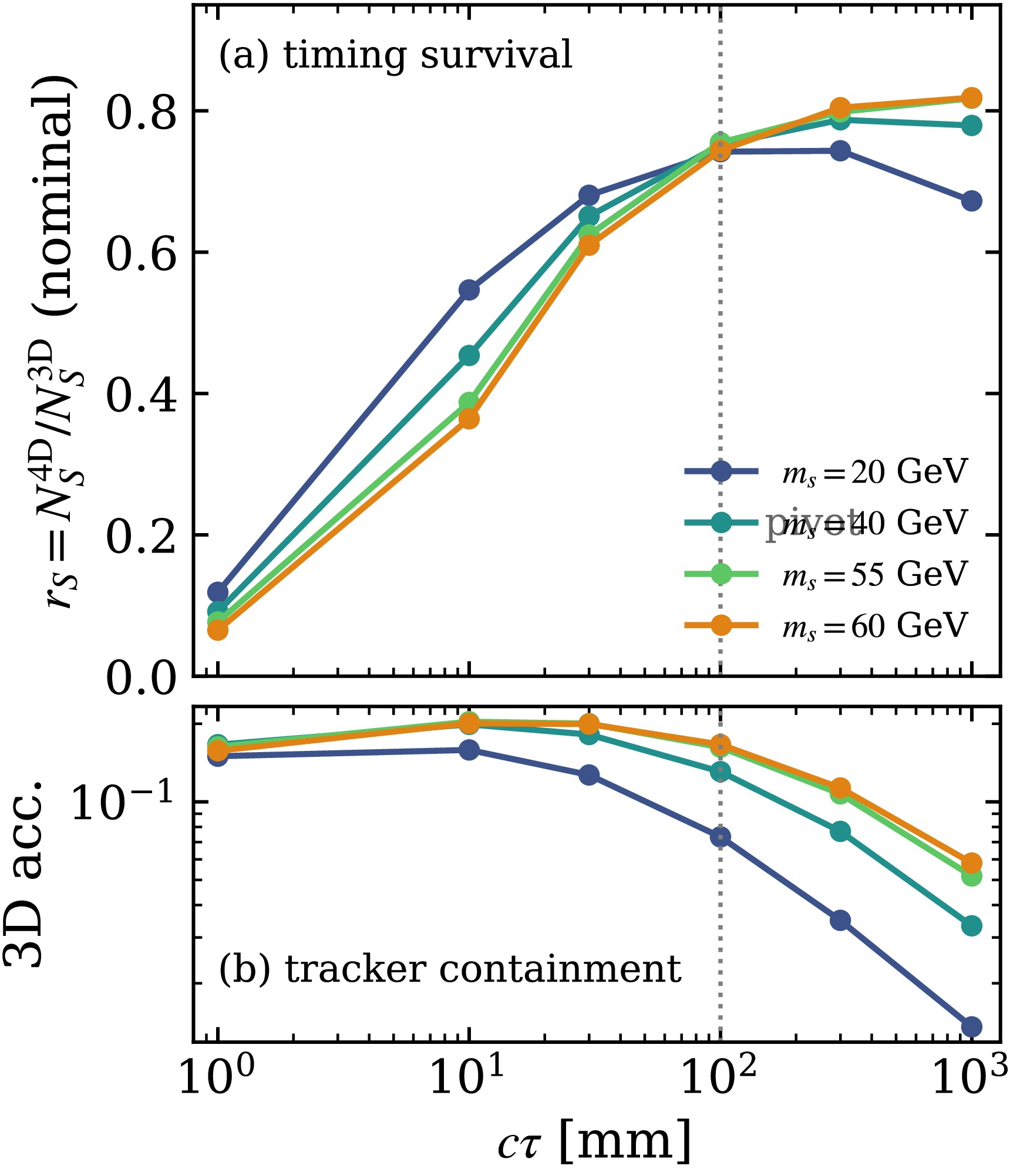
Figure A2. (color online) (a) Nominal 4D signal timing survival,
$ r_S=N^{\rm 4D}_S/N^{\rm 3D}_S $ , as a function of decay length for the four scalar masses; the curves converge at$ c\tau\simeq100 \,{\rm{mm}} $ (dotted line), where the mass ordering of the gain reverses. (b) Spatial (3D) acceptance,$ N^{\rm 3D}_S/N_{{\rm{gen}}} $ , which decreases most rapidly for the lightest, most boosted scalar at long$ c\tau $ . Since$ r_B $ is common to all masses, panel (a) shows the full mass dependence of$ {\cal{G}} $ . -
This supplement presents the selection cutflow (Table A1), the statistical procedure used to derive the projected limits, and the robustness studies referenced in the main text: the timed-SV efficiency underlying the barrel-timing configuration (Fig. A1), the mass decomposition of the timing survival that yields the gain pivot (Fig. A2), the start-time reference multiplicity (Fig. A3), and the illustrative branching-ratio limit together with its dependence on the assumed background-normalization uncertainty
$ \kappa_b $ (Figs. A4 and A5). All results use the same$ 2.2\times10^{6} $ -event QCD sample and the full signal grid ($ m_s\in\{20,40,55,60\} \,{\rm{GeV}} $ ,$ c\tau\in\{1,10,30,100,300,1000\} \,{\rm{mm}} $ ) as in the main analysis, with the barrel timing layer ($ |\eta|<1.48 $ ,$ \sigma_t=30 \,{\rm{ps}} $ ,$ p_T>0.7 \,{\rm{GeV}} $ ), and assume$ {\rm{BR}}(s\to b\bar b)=1 $ throughout.
Figure A2. (color online) (a) Nominal 4D signal timing survival,
$ r_S=N^{\rm 4D}_S/N^{\rm 3D}_S $ , as a function of decay length for the four scalar masses; the curves converge at$ c\tau\simeq100 \,{\rm{mm}} $ (dotted line), where the mass ordering of the gain reverses. (b) Spatial (3D) acceptance,$ N^{\rm 3D}_S/N_{{\rm{gen}}} $ , which decreases most rapidly for the lightest, most boosted scalar at long$ c\tau $ . Since$ r_B $ is common to all masses, panel (a) shows the full mass dependence of$ {\cal{G}} $ . -
This supplement presents the selection cutflow (Table A1), the statistical procedure used to derive the projected limits, and the robustness studies referenced in the main text: the timed-SV efficiency underlying the barrel-timing configuration (Fig. A1), the mass decomposition of the timing survival that yields the gain pivot (Fig. A2), the start-time reference multiplicity (Fig. A3), and the illustrative branching-ratio limit together with its dependence on the assumed background-normalization uncertainty
$ \kappa_b $ (Figs. A4 and A5). All results use the same$ 2.2\times10^{6} $ -event QCD sample and the full signal grid ($ m_s\in\{20,40,55,60\} \,{\rm{GeV}} $ ,$ c\tau\in\{1,10,30,100,300,1000\} \,{\rm{mm}} $ ) as in the main analysis, with the barrel timing layer ($ |\eta|<1.48 $ ,$ \sigma_t=30 \,{\rm{ps}} $ ,$ p_T>0.7 \,{\rm{GeV}} $ ), and assume$ {\rm{BR}}(s\to b\bar b)=1 $ throughout.
Figure A2. (color online) (a) Nominal 4D signal timing survival,
$ r_S=N^{\rm 4D}_S/N^{\rm 3D}_S $ , as a function of decay length for the four scalar masses; the curves converge at$ c\tau\simeq100 \,{\rm{mm}} $ (dotted line), where the mass ordering of the gain reverses. (b) Spatial (3D) acceptance,$ N^{\rm 3D}_S/N_{{\rm{gen}}} $ , which decreases most rapidly for the lightest, most boosted scalar at long$ c\tau $ . Since$ r_B $ is common to all masses, panel (a) shows the full mass dependence of$ {\cal{G}} $ . -
Statistical procedure—The projected limits use a single-bin counting likelihood
$ {\cal{L}}(n\,|\,\mu,\theta_b)= {\rm{Pois}} \big(n\,\big|\,\mu\,s + b\,(1+\kappa_b\,\theta_b)\big)\, \exp \big(-\theta_b^2/2\big), $
(A1) where s and b denote the expected signal and background yields at
$ 3000 \;{\rm{fb}}^{-1} $ , respectively. Here, μ is the signal strength—linear in$ {\rm{BR}}(h\to ss) $ for the fixed assumption$ {\rm{BR}}(s\to b\bar b)=1 $ —and$ \theta_b $ is a nuisance parameter constrained by a unit Gaussian, such that$ \kappa_b $ specifies the fractional background-normalization uncertainty. The expected 95% CL upper limit is obtained from the asymptotic$ {\rm{CL}}_s $ test statistic [38, 39], evaluated on the Asimov dataset$ n=b $ , which also defines the$ \pm1,2\sigma $ bands in Fig. A4. For$ \kappa_b=0 $ , the limit is purely statistical. The Monte Carlo statistical uncertainty on the optimized background tail ($ \simeq $ 7%, Table A1) is propagated as an additional contribution to b. -
Statistical procedure—The projected limits use a single-bin counting likelihood
$ {\cal{L}}(n\,|\,\mu,\theta_b)= {\rm{Pois}} \big(n\,\big|\,\mu\,s + b\,(1+\kappa_b\,\theta_b)\big)\, \exp \big(-\theta_b^2/2\big), $
(A1) where s and b denote the expected signal and background yields at
$ 3000 \;{\rm{fb}}^{-1} $ , respectively. Here, μ is the signal strength—linear in$ {\rm{BR}}(h\to ss) $ for the fixed assumption$ {\rm{BR}}(s\to b\bar b)=1 $ —and$ \theta_b $ is a nuisance parameter constrained by a unit Gaussian, such that$ \kappa_b $ specifies the fractional background-normalization uncertainty. The expected 95% CL upper limit is obtained from the asymptotic$ {\rm{CL}}_s $ test statistic [38, 39], evaluated on the Asimov dataset$ n=b $ , which also defines the$ \pm1,2\sigma $ bands in Fig. A4. For$ \kappa_b=0 $ , the limit is purely statistical. The Monte Carlo statistical uncertainty on the optimized background tail ($ \simeq $ 7%, Table A1) is propagated as an additional contribution to b. -
Statistical procedure—The projected limits use a single-bin counting likelihood
$ {\cal{L}}(n\,|\,\mu,\theta_b)= {\rm{Pois}} \big(n\,\big|\,\mu\,s + b\,(1+\kappa_b\,\theta_b)\big)\, \exp \big(-\theta_b^2/2\big), $
(A1) where s and b denote the expected signal and background yields at
$ 3000 \;{\rm{fb}}^{-1} $ , respectively. Here, μ is the signal strength—linear in$ {\rm{BR}}(h\to ss) $ for the fixed assumption$ {\rm{BR}}(s\to b\bar b)=1 $ —and$ \theta_b $ is a nuisance parameter constrained by a unit Gaussian, such that$ \kappa_b $ specifies the fractional background-normalization uncertainty. The expected 95% CL upper limit is obtained from the asymptotic$ {\rm{CL}}_s $ test statistic [38, 39], evaluated on the Asimov dataset$ n=b $ , which also defines the$ \pm1,2\sigma $ bands in Fig. A4. For$ \kappa_b=0 $ , the limit is purely statistical. The Monte Carlo statistical uncertainty on the optimized background tail ($ \simeq $ 7%, Table A1) is propagated as an additional contribution to b. -
Selection cutflow—Table A1 presents the cutflow at the benchmark point for the signal and the dominant QCD background.
-
Selection cutflow—Table A1 presents the cutflow at the benchmark point for the signal and the dominant QCD background.
-
Selection cutflow—Table A1 presents the cutflow at the benchmark point for the signal and the dominant QCD background.
-
Timed-SV efficiency—The four-dimensional selection requires that the displaced-vertex tracks themselves carry timing information, which is possible only within the barrel acceptance. Figure A1 shows, for the spatially selected (3D) vertices, the fraction that retain at least one, two, or three timed SV tracks as a function of
$ c\tau $ ; each band represents the envelope across the four scalar masses, and the line denotes their mean. The efficiency for$ \geqslant1 $ timed track is$ 80\text{–}$ 87% over the entire grid, with a mass spread of only a few percent and no anomalously low point. This indicates that, in this fast-simulation setup, the central SV tracks—which recoil against the forward tag jets—fall within the barrel coverage across the grid. The mild increase with$ c\tau $ follows the increasing collimation and momentum of the decay products, while the slight broadening at the longest lifetime is driven by the lightest, most boosted scalar. Requiring$ \geqslant2 $ or$ \geqslant3 $ timed tracks lowers the efficiency by only a few percent, indicating that$ \Delta T_{{\rm{SV}}} $ is reconstructed from several tracks rather than a single one. -
Timed-SV efficiency—The four-dimensional selection requires that the displaced-vertex tracks themselves carry timing information, which is possible only within the barrel acceptance. Figure A1 shows, for the spatially selected (3D) vertices, the fraction that retain at least one, two, or three timed SV tracks as a function of
$ c\tau $ ; each band represents the envelope across the four scalar masses, and the line denotes their mean. The efficiency for$ \geqslant1 $ timed track is$ 80\text{–}$ 87% over the entire grid, with a mass spread of only a few percent and no anomalously low point. This indicates that, in this fast-simulation setup, the central SV tracks—which recoil against the forward tag jets—fall within the barrel coverage across the grid. The mild increase with$ c\tau $ follows the increasing collimation and momentum of the decay products, while the slight broadening at the longest lifetime is driven by the lightest, most boosted scalar. Requiring$ \geqslant2 $ or$ \geqslant3 $ timed tracks lowers the efficiency by only a few percent, indicating that$ \Delta T_{{\rm{SV}}} $ is reconstructed from several tracks rather than a single one. -
Timed-SV efficiency—The four-dimensional selection requires that the displaced-vertex tracks themselves carry timing information, which is possible only within the barrel acceptance. Figure A1 shows, for the spatially selected (3D) vertices, the fraction that retain at least one, two, or three timed SV tracks as a function of
$ c\tau $ ; each band represents the envelope across the four scalar masses, and the line denotes their mean. The efficiency for$ \geqslant1 $ timed track is$ 80\text{–}$ 87% over the entire grid, with a mass spread of only a few percent and no anomalously low point. This indicates that, in this fast-simulation setup, the central SV tracks—which recoil against the forward tag jets—fall within the barrel coverage across the grid. The mild increase with$ c\tau $ follows the increasing collimation and momentum of the decay products, while the slight broadening at the longest lifetime is driven by the lightest, most boosted scalar. Requiring$ \geqslant2 $ or$ \geqslant3 $ timed tracks lowers the efficiency by only a few percent, indicating that$ \Delta T_{{\rm{SV}}} $ is reconstructed from several tracks rather than a single one. -
Mass-pivot decomposition — Because
$ r_B $ is common to all signal points, the mass dependence of the gain$ {\cal{G}}=r_S/\sqrt{r_B} $ resides entirely in the signal timing survival$ r_S(m_s, c\tau) $ . Figure A2(a) shows$ r_S $ at the nominal working point for the four masses. The curves intersect at$ c\tau\simeq100 \,{\rm{mm}} $ , where all four converge to$ r_S\simeq0.74\text{–}0.76 $ . At shorter lifetimes, the larger boost of the lighter scalar ($ \beta\gamma\simeq p_s/ m_s $ ) carries more decays beyond the displacement and time thresholds, so the lighter mass has the larger$ r_S $ . At longer lifetimes, the same boost drives the light scalar out of the tracker, and the heavier, slower scalar retains the larger$ r_S $ . Figure A2(b) shows the spatial (3D) acceptance, which decreases most rapidly for the lightest scalar at long$ c\tau $ , quantifying the tracker-containment leakage that drives the reversal. The pivot in$ {\cal{G}} $ is therefore the kinematic point at which boost-enhanced timing survival and boost-induced containment loss balance, rather than an artifact of the timing threshold. -
Mass-pivot decomposition — Because
$ r_B $ is common to all signal points, the mass dependence of the gain$ {\cal{G}}=r_S/\sqrt{r_B} $ resides entirely in the signal timing survival$ r_S(m_s, c\tau) $ . Figure A2(a) shows$ r_S $ at the nominal working point for the four masses. The curves intersect at$ c\tau\simeq100 \,{\rm{mm}} $ , where all four converge to$ r_S\simeq0.74\text{–}0.76 $ . At shorter lifetimes, the larger boost of the lighter scalar ($ \beta\gamma\simeq p_s/ m_s $ ) carries more decays beyond the displacement and time thresholds, so the lighter mass has the larger$ r_S $ . At longer lifetimes, the same boost drives the light scalar out of the tracker, and the heavier, slower scalar retains the larger$ r_S $ . Figure A2(b) shows the spatial (3D) acceptance, which decreases most rapidly for the lightest scalar at long$ c\tau $ , quantifying the tracker-containment leakage that drives the reversal. The pivot in$ {\cal{G}} $ is therefore the kinematic point at which boost-enhanced timing survival and boost-induced containment loss balance, rather than an artifact of the timing threshold. -
Mass-pivot decomposition — Because
$ r_B $ is common to all signal points, the mass dependence of the gain$ {\cal{G}}=r_S/\sqrt{r_B} $ resides entirely in the signal timing survival$ r_S(m_s, c\tau) $ . Figure A2(a) shows$ r_S $ at the nominal working point for the four masses. The curves intersect at$ c\tau\simeq100 \,{\rm{mm}} $ , where all four converge to$ r_S\simeq0.74\text{–}0.76 $ . At shorter lifetimes, the larger boost of the lighter scalar ($ \beta\gamma\simeq p_s/ m_s $ ) carries more decays beyond the displacement and time thresholds, so the lighter mass has the larger$ r_S $ . At longer lifetimes, the same boost drives the light scalar out of the tracker, and the heavier, slower scalar retains the larger$ r_S $ . Figure A2(b) shows the spatial (3D) acceptance, which decreases most rapidly for the lightest scalar at long$ c\tau $ , quantifying the tracker-containment leakage that drives the reversal. The pivot in$ {\cal{G}} $ is therefore the kinematic point at which boost-enhanced timing survival and boost-induced containment loss balance, rather than an artifact of the timing threshold. -
Start-time reference availability—The event start time
$ t_0 $ is determined from prompt central reference tracks. Across the full mass–lifetime grid, a usable reference ($ N_{{\rm{ref}}}\geqslant1 $ ) is found in$ 94\text{–}$ 96% of signal events, with a mean multiplicity of$ \langle N_{{\rm{ref}}}\rangle\simeq15 $ (Fig. A3). The$ 4\%\text{–}$ 6% of events without a prompt reference cannot define$ t_0 $ and are therefore removed only from the 4D selection, leaving the 3D baseline—and hence the denominator of$ {\cal{G}} $ —unchanged. This mean multiplicity yields a statistical start-time precision of$ \sigma_t/\sqrt{N_{{\rm{ref}}}}\sim8 \;{\rm{ps}} $ for$ \sigma_t=30 \;{\rm{ps}} $ . -
Start-time reference availability—The event start time
$ t_0 $ is determined from prompt central reference tracks. Across the full mass–lifetime grid, a usable reference ($ N_{{\rm{ref}}}\geqslant1 $ ) is found in$ 94\text{–}$ 96% of signal events, with a mean multiplicity of$ \langle N_{{\rm{ref}}}\rangle\simeq15 $ (Fig. A3). The$ 4\%\text{–}$ 6% of events without a prompt reference cannot define$ t_0 $ and are therefore removed only from the 4D selection, leaving the 3D baseline—and hence the denominator of$ {\cal{G}} $ —unchanged. This mean multiplicity yields a statistical start-time precision of$ \sigma_t/\sqrt{N_{{\rm{ref}}}}\sim8 \;{\rm{ps}} $ for$ \sigma_t=30 \;{\rm{ps}} $ . -
Start-time reference availability—The event start time
$ t_0 $ is determined from prompt central reference tracks. Across the full mass–lifetime grid, a usable reference ($ N_{{\rm{ref}}}\geqslant1 $ ) is found in$ 94\text{–}$ 96% of signal events, with a mean multiplicity of$ \langle N_{{\rm{ref}}}\rangle\simeq15 $ (Fig. A3). The$ 4\%\text{–}$ 6% of events without a prompt reference cannot define$ t_0 $ and are therefore removed only from the 4D selection, leaving the 3D baseline—and hence the denominator of$ {\cal{G}} $ —unchanged. This mean multiplicity yields a statistical start-time precision of$ \sigma_t/\sqrt{N_{{\rm{ref}}}}\sim8 \;{\rm{ps}} $ for$ \sigma_t=30 \;{\rm{ps}} $ . -
Illustrative branching-ratio limit—Figure A4 shows the statistics-limited projection for
$ m_s=60 \,{\rm{GeV}} $ discussed in the main text, for the 3D-only and optimized-4D selections; the absolute scale is an idealized lower bound set by the background normalization. -
Illustrative branching-ratio limit—Figure A4 shows the statistics-limited projection for
$ m_s=60 \,{\rm{GeV}} $ discussed in the main text, for the 3D-only and optimized-4D selections; the absolute scale is an idealized lower bound set by the background normalization. -
Illustrative branching-ratio limit—Figure A4 shows the statistics-limited projection for
$ m_s=60 \,{\rm{GeV}} $ discussed in the main text, for the 3D-only and optimized-4D selections; the absolute scale is an idealized lower bound set by the background normalization. -
Background-normalization dependence—Because a phenomenological projection cannot determine the absolute QCD normalization, the limit is quoted for a range of assumed fractional background uncertainties
$ \kappa_b $ . Figure A5 overlays the median upper limit at$ m_s= 60 \;{\rm{GeV}} $ for the 3D-only and optimized-4D selections at$ \kappa_b=0 $ (statistics only), 1%, and 5%. In the statistics-limited case ($ \kappa_b=0 $ ), the optimized selection improves the limit by the gain factor ($ \simeq10 $ at the benchmark). Once a normalization uncertainty is included, the spatial limit rises above unity across the entire lifetime range. Thus, the 3D search excludes no physically allowed branching ratio, whereas the optimized-4D limit, whose background is$ \simeq500 $ times smaller, remains below unity and still excludes$ {\rm{BR}}\lesssim0.1 $ for$ \kappa_b $ =1% ($ c\tau\gtrsim10 \;{\rm{mm}} $ ) and$ {\rm{BR}}\lesssim0.7 $ for$ \kappa_b$ =5% ($ c\tau\gtrsim30 \;{\rm{mm}} $ ). At the benchmark$ c\tau=100 \;{\rm{mm}} $ , the two median limits differ by a factor of$ \simeq216 $ ($ \kappa_b$ =1%) and$ \simeq223 $ ($ \kappa_b $ =5%); where both lie above$ {\rm{BR}}=1 $ , this ratio measures relative sensitivity rather than exclusion power. The timing advantage thus grows with the background uncertainty—the regime expected in a real measurement—and is what keeps the search viable. The comparison assumes the same fractional$ \kappa_b $ for the 3D and 4D selections. In a real analysis, however,$ \kappa_b $ would instead be set by the control-region statistics and transfer-factor systematics of each selection, which need not coincide because the 4D background composition differs from that of the 3D selection. -
Background-normalization dependence—Because a phenomenological projection cannot determine the absolute QCD normalization, the limit is quoted for a range of assumed fractional background uncertainties
$ \kappa_b $ . Figure A5 overlays the median upper limit at$ m_s= 60 \;{\rm{GeV}} $ for the 3D-only and optimized-4D selections at$ \kappa_b=0 $ (statistics only), 1%, and 5%. In the statistics-limited case ($ \kappa_b=0 $ ), the optimized selection improves the limit by the gain factor ($ \simeq10 $ at the benchmark). Once a normalization uncertainty is included, the spatial limit rises above unity across the entire lifetime range. Thus, the 3D search excludes no physically allowed branching ratio, whereas the optimized-4D limit, whose background is$ \simeq500 $ times smaller, remains below unity and still excludes$ {\rm{BR}}\lesssim0.1 $ for$ \kappa_b $ =1% ($ c\tau\gtrsim10 \;{\rm{mm}} $ ) and$ {\rm{BR}}\lesssim0.7 $ for$ \kappa_b$ =5% ($ c\tau\gtrsim30 \;{\rm{mm}} $ ). At the benchmark$ c\tau=100 \;{\rm{mm}} $ , the two median limits differ by a factor of$ \simeq216 $ ($ \kappa_b$ =1%) and$ \simeq223 $ ($ \kappa_b $ =5%); where both lie above$ {\rm{BR}}=1 $ , this ratio measures relative sensitivity rather than exclusion power. The timing advantage thus grows with the background uncertainty—the regime expected in a real measurement—and is what keeps the search viable. The comparison assumes the same fractional$ \kappa_b $ for the 3D and 4D selections. In a real analysis, however,$ \kappa_b $ would instead be set by the control-region statistics and transfer-factor systematics of each selection, which need not coincide because the 4D background composition differs from that of the 3D selection. -
Background-normalization dependence—Because a phenomenological projection cannot determine the absolute QCD normalization, the limit is quoted for a range of assumed fractional background uncertainties
$ \kappa_b $ . Figure A5 overlays the median upper limit at$ m_s= 60 \;{\rm{GeV}} $ for the 3D-only and optimized-4D selections at$ \kappa_b=0 $ (statistics only), 1%, and 5%. In the statistics-limited case ($ \kappa_b=0 $ ), the optimized selection improves the limit by the gain factor ($ \simeq10 $ at the benchmark). Once a normalization uncertainty is included, the spatial limit rises above unity across the entire lifetime range. Thus, the 3D search excludes no physically allowed branching ratio, whereas the optimized-4D limit, whose background is$ \simeq500 $ times smaller, remains below unity and still excludes$ {\rm{BR}}\lesssim0.1 $ for$ \kappa_b $ =1% ($ c\tau\gtrsim10 \;{\rm{mm}} $ ) and$ {\rm{BR}}\lesssim0.7 $ for$ \kappa_b$ =5% ($ c\tau\gtrsim30 \;{\rm{mm}} $ ). At the benchmark$ c\tau=100 \;{\rm{mm}} $ , the two median limits differ by a factor of$ \simeq216 $ ($ \kappa_b$ =1%) and$ \simeq223 $ ($ \kappa_b $ =5%); where both lie above$ {\rm{BR}}=1 $ , this ratio measures relative sensitivity rather than exclusion power. The timing advantage thus grows with the background uncertainty—the regime expected in a real measurement—and is what keeps the search viable. The comparison assumes the same fractional$ \kappa_b $ for the 3D and 4D selections. In a real analysis, however,$ \kappa_b $ would instead be set by the control-region statistics and transfer-factor systematics of each selection, which need not coincide because the 4D background composition differs from that of the 3D selection. -
Velocity approximation—Setting
$ \beta_i=1 $ in$ t_i^{{\rm{SV}}}=t_i^{{\rm{hit}}}- L_i/(\beta_i c) $ introduces a bias into the reconstructed production time of a charged hadron with mass$ m_i $ and momentum$ p_i $ by$ \Delta t_i=\frac{L_i}{c} \left(\frac{1}{\beta_i}-1\right) =\frac{L_i}{c} \left(\frac{\sqrt{p_i^2+m_i^2}}{p_i}-1\right) \simeq\frac{L_i}{c}\,\frac{m_i^2}{2p_i^2}, $
(A2) a positive shift that increases for low-momentum tracks (Fig. A6). For the path length to the barrel,
$ L\simeq1.15\; $ m, the bias for a pion is$ \simeq37 \;{\rm{ps}} $ at$ p_T=1 \;{\rm{GeV}} $ ,$ \simeq9 \,{\rm{ps}} $ at$ 2 \;{\rm{GeV}} $ , and$ \lesssim2 \;{\rm{ps}} $ above$ 5 \;{\rm{GeV}} $ ; kaons and protons exhibit larger biases but constitute only a small fraction of the tracks from a$ b\bar b $ system. The bias is, however, common mode: the prompt reference tracks that determine$ t_0 $ and the displaced-vertex tracks are both charged hadrons treated with$ \beta=1 $ and have similar momentum spectra, so it largely cancels in$ \Delta T_{{\rm{SV}}}=\langle t^{{\rm{SV}}}\rangle_{{\rm{SV}}}-t_0 $ , leaving only the residual difference between the two populations—at the few-ps level, well below$ \sigma_t=30 \;{\rm{ps}} $ . We propagate this residual by varying the correction over the track-momentum-dependent hadron-mass envelope (pion to proton); it is included in the systematic budget and, being much smaller than$ \sigma_t $ , neither shifts the break-even point appreciably nor promotes a prompt vertex beyond the$ 3 \sigma_t $ threshold. Because the shift is positive for signal and background vertices alike, it cannot by itself convert a prompt heavy-flavour vertex into a coherent late signal: the common component is removed by the$ t_0 $ subtraction and by the late-track-fraction requirement$ f_{{\rm{late}}} $ , whereas a genuine long-lived delay ($ \Delta T_{{\rm{SV}}}\gtrsim100 \;{\rm{ps}} $ for$ c\tau\gtrsim30 \;{\rm{mm}} $ ) far exceeds$ \Delta t_i $ . Quantitatively, the same reasoning bounds the effect on the background estimate: because the residual is only a few ps while the nominal cut is set at$ 3 \sigma_t=90 \;{\rm{ps}} $ , it shifts a negligible fraction of the prompt QCD vertices—whose$ \Delta T_{{\rm{SV}}} $ peaks near zero (median$ 25 \;{\rm{ps}} $ )—across the timing selection. Thus, the induced change in the background timing-survival$ r_B $ is contained within the hadron-mass-envelope systematic and is far smaller than the pileup and start-time systematics on$ r_B $ . The gain$ {\cal{G}}=r_S/\sqrt{r_B} $ is therefore unchanged at the quoted precision, and because$ r_B $ is common to every mass, the mass pivot of Fig. 2 is left intact. -
Velocity approximation—Setting
$ \beta_i=1 $ in$ t_i^{{\rm{SV}}}=t_i^{{\rm{hit}}}- L_i/(\beta_i c) $ introduces a bias into the reconstructed production time of a charged hadron with mass$ m_i $ and momentum$ p_i $ by$ \Delta t_i=\frac{L_i}{c} \left(\frac{1}{\beta_i}-1\right) =\frac{L_i}{c} \left(\frac{\sqrt{p_i^2+m_i^2}}{p_i}-1\right) \simeq\frac{L_i}{c}\,\frac{m_i^2}{2p_i^2}, $
(A2) a positive shift that increases for low-momentum tracks (Fig. A6). For the path length to the barrel,
$ L\simeq1.15\; $ m, the bias for a pion is$ \simeq37 \;{\rm{ps}} $ at$ p_T=1 \;{\rm{GeV}} $ ,$ \simeq9 \,{\rm{ps}} $ at$ 2 \;{\rm{GeV}} $ , and$ \lesssim2 \;{\rm{ps}} $ above$ 5 \;{\rm{GeV}} $ ; kaons and protons exhibit larger biases but constitute only a small fraction of the tracks from a$ b\bar b $ system. The bias is, however, common mode: the prompt reference tracks that determine$ t_0 $ and the displaced-vertex tracks are both charged hadrons treated with$ \beta=1 $ and have similar momentum spectra, so it largely cancels in$ \Delta T_{{\rm{SV}}}=\langle t^{{\rm{SV}}}\rangle_{{\rm{SV}}}-t_0 $ , leaving only the residual difference between the two populations—at the few-ps level, well below$ \sigma_t=30 \;{\rm{ps}} $ . We propagate this residual by varying the correction over the track-momentum-dependent hadron-mass envelope (pion to proton); it is included in the systematic budget and, being much smaller than$ \sigma_t $ , neither shifts the break-even point appreciably nor promotes a prompt vertex beyond the$ 3 \sigma_t $ threshold. Because the shift is positive for signal and background vertices alike, it cannot by itself convert a prompt heavy-flavour vertex into a coherent late signal: the common component is removed by the$ t_0 $ subtraction and by the late-track-fraction requirement$ f_{{\rm{late}}} $ , whereas a genuine long-lived delay ($ \Delta T_{{\rm{SV}}}\gtrsim100 \;{\rm{ps}} $ for$ c\tau\gtrsim30 \;{\rm{mm}} $ ) far exceeds$ \Delta t_i $ . Quantitatively, the same reasoning bounds the effect on the background estimate: because the residual is only a few ps while the nominal cut is set at$ 3 \sigma_t=90 \;{\rm{ps}} $ , it shifts a negligible fraction of the prompt QCD vertices—whose$ \Delta T_{{\rm{SV}}} $ peaks near zero (median$ 25 \;{\rm{ps}} $ )—across the timing selection. Thus, the induced change in the background timing-survival$ r_B $ is contained within the hadron-mass-envelope systematic and is far smaller than the pileup and start-time systematics on$ r_B $ . The gain$ {\cal{G}}=r_S/\sqrt{r_B} $ is therefore unchanged at the quoted precision, and because$ r_B $ is common to every mass, the mass pivot of Fig. 2 is left intact. -
Velocity approximation—Setting
$ \beta_i=1 $ in$ t_i^{{\rm{SV}}}=t_i^{{\rm{hit}}}- L_i/(\beta_i c) $ introduces a bias into the reconstructed production time of a charged hadron with mass$ m_i $ and momentum$ p_i $ by$ \Delta t_i=\frac{L_i}{c} \left(\frac{1}{\beta_i}-1\right) =\frac{L_i}{c} \left(\frac{\sqrt{p_i^2+m_i^2}}{p_i}-1\right) \simeq\frac{L_i}{c}\,\frac{m_i^2}{2p_i^2}, $
(A2) a positive shift that increases for low-momentum tracks (Fig. A6). For the path length to the barrel,
$ L\simeq1.15\; $ m, the bias for a pion is$ \simeq37 \;{\rm{ps}} $ at$ p_T=1 \;{\rm{GeV}} $ ,$ \simeq9 \,{\rm{ps}} $ at$ 2 \;{\rm{GeV}} $ , and$ \lesssim2 \;{\rm{ps}} $ above$ 5 \;{\rm{GeV}} $ ; kaons and protons exhibit larger biases but constitute only a small fraction of the tracks from a$ b\bar b $ system. The bias is, however, common mode: the prompt reference tracks that determine$ t_0 $ and the displaced-vertex tracks are both charged hadrons treated with$ \beta=1 $ and have similar momentum spectra, so it largely cancels in$ \Delta T_{{\rm{SV}}}=\langle t^{{\rm{SV}}}\rangle_{{\rm{SV}}}-t_0 $ , leaving only the residual difference between the two populations—at the few-ps level, well below$ \sigma_t=30 \;{\rm{ps}} $ . We propagate this residual by varying the correction over the track-momentum-dependent hadron-mass envelope (pion to proton); it is included in the systematic budget and, being much smaller than$ \sigma_t $ , neither shifts the break-even point appreciably nor promotes a prompt vertex beyond the$ 3 \sigma_t $ threshold. Because the shift is positive for signal and background vertices alike, it cannot by itself convert a prompt heavy-flavour vertex into a coherent late signal: the common component is removed by the$ t_0 $ subtraction and by the late-track-fraction requirement$ f_{{\rm{late}}} $ , whereas a genuine long-lived delay ($ \Delta T_{{\rm{SV}}}\gtrsim100 \;{\rm{ps}} $ for$ c\tau\gtrsim30 \;{\rm{mm}} $ ) far exceeds$ \Delta t_i $ . Quantitatively, the same reasoning bounds the effect on the background estimate: because the residual is only a few ps while the nominal cut is set at$ 3 \sigma_t=90 \;{\rm{ps}} $ , it shifts a negligible fraction of the prompt QCD vertices—whose$ \Delta T_{{\rm{SV}}} $ peaks near zero (median$ 25 \;{\rm{ps}} $ )—across the timing selection. Thus, the induced change in the background timing-survival$ r_B $ is contained within the hadron-mass-envelope systematic and is far smaller than the pileup and start-time systematics on$ r_B $ . The gain$ {\cal{G}}=r_S/\sqrt{r_B} $ is therefore unchanged at the quoted precision, and because$ r_B $ is common to every mass, the mass pivot of Fig. 2 is left intact.
Vector-boson-fusion timing references for four-dimensional displaced-vertex searches
- Received Date: 2026-06-23
- Available Online: 2026-11-15
Abstract: Long-lived particles that decay inside the tracker are searched for via the spatial displacement of their decay vertices. However, the same decays also arrive late, providing a handle made available by a precision timing layer at the HL-LHC that displaced-vertex searches do not exploit. We study the exotic decay of a Higgs boson produced through vector-boson fusion (VBF), $ pp\to hjj $ with $ h\to ss $, in which the long-lived scalar decays as $ s\to b\bar b $, and use the VBF tag jets to identify the hard-scatter vertex. Its prompt central tracks, timed by a CMS-MTD-like barrel layer that also times the central tracks of the displaced vertex, define a per-event start time, turning each displaced vertex into a four-dimensional object. Because a fast simulation cannot determine the absolute normalization of the heavy-flavour and instrumental displaced-vertex backgrounds, we take as the primary result a normalization-free figure of merit: the ratio of the timing-enhanced sensitivity to the spatial-only sensitivity. Adding the timing layer improves this ratio by a factor of $ \simeq2.8 $ at a nominal working point and by up to an order of magnitude for a tighter delayed-vertex requirement, because the heavy-flavour background that survives the spatial selection is prompt in collision time. The improvement increases with decay length, extending sensitivity into the long-lifetime regime in which purely spatial searches lose tracker acceptance. The gain is essentially mass-independent at a decay length of $ c\tau\simeq100 \,{\rm{mm}} $, where the trend with scalar mass reverses: lighter scalars benefit more at short lifetimes because of their larger boost, whereas heavier scalars benefit more at long lifetimes as the lighter states leak out of the tracker.



 DownLoad: