Decoherence Effects on Primordial Black Holes and Scalar-Induced Gravitational Waves

Primordial black holes (PBHs) offer a rare observational handle on the small-scale primordial Universe [1]. The cosmic microwave background (CMB) probes curvature perturbations on very large scales, whereas PBHs are sensitive to much shorter wavelengths that re-enter the Hubble radius during the radiation era. If the primordial curvature perturbation is sufficiently enhanced on these scales, rare overdense regions may collapse gravitationally to form black holes. This makes PBHs a useful probe of inflationary dynamics far beyond the CMB window [2−6]. At the same time, PBH formation is not determined by the power spectrum alone. The collapse is a classical nonlinear process that depends on the density contrast, the compaction function, the equation of state, and the shape of the perturbation profile [7−10]. This distinction is important: the mechanism that generates large primordial fluctuations belongs to inflationary physics, whereas the final collapse into PBHs is governed by classical gravitational dynamics at horizon re-entry.

One simple and efficient way to enhance the scalar power spectrum is to include a short non-attractor phase during inflation. A typical example is ultra-slow-roll (USR) evolution, in which the inflaton potential becomes locally very flat and the inflaton velocity is rapidly damped by the expansion of the Universe [11, 12]. During this stage, the slow-roll parameter decreases approximately as $ \epsilon\propto a^{-6} $, and the would-be decaying mode of the curvature perturbation grows outside the Hubble radius. As a result, the curvature perturbation can be amplified by many orders of magnitude over a narrow range of scales. This provides a natural route to PBH formation and also sources a stochastic scalar-induced gravitational-wave (SIGW) background when the enhanced scalar modes re-enter the horizon during radiation domination [13−17]. For related higher-dimensional scenarios involving primordial black holes and scalar-induced gravitational waves, see Refs. [18, 19].

The SIGW signal is especially important because it provides an indirect probe of the same small-scale scalar fluctuations responsible for PBH production. Even if PBHs constitute only a small fraction of the dark matter, the accompanying induced gravitational waves may be observable by pulsar timing arrays, space-based detectors, or ground-based interferometers, depending on the peak scale of the scalar spectrum [20−24]. In this sense, PBHs and SIGWs form a closely related pair of observables: PBHs probe the rare tail of the density fluctuations, while SIGWs probe the two-point scalar covariance through the second-order tensor source.

There is, however, a quantum question underlying this classical PBH/SIGW picture. The primordial curvature perturbations that later seed PBHs are believed to originate from quantum vacuum fluctuations generated during inflation and subsequently stretched to cosmological scales [25−27]. At the level of linear cosmological perturbation theory, each pair of opposite Fourier modes, $ ({\boldsymbol{k}}, -{\boldsymbol{k}}) $, evolves into a two-mode squeezed Gaussian quantum state due to parametric amplification by the expanding background [28−31]. After horizon exit, the squeezing parameter becomes very large, and the perturbations behave in many practical respects like a classical stochastic field, although the covariance matrix continues to encode information about their quantum origin. This issue is closely related to the quantum-to-classical transition of inflationary perturbations, which has been extensively studied using squeezing, decoherence, and the emergence of classical stochastic correlations [30−32].

Quantum-information theory provides a useful language for making this question more precise. Entanglement is one possible measure of quantumness, but it is not the only one. In mixed Gaussian states, entanglement can disappear while weaker quantum correlations remain. Gaussian quantum discord is designed to capture this broader class of quantum correlations [33−36]. In cosmology, such covariance-matrix diagnostics have been used to study the quantum nature of inflationary perturbations and their behavior under decoherence [37−41]. These ideas suggest that PBH-producing modes should not be viewed solely as a classical random field from the outset; rather, their quantum origin and subsequent decoherence may leave useful information in the Gaussian covariance structure.

The aim of this work is to apply this viewpoint to the PBH and SIGW problem in a conservative way. We do not propose that quantum discord replaces the PBH collapse threshold. PBH formation remains a classical threshold process: a sufficiently large density perturbation must re-enter the Hubble radius and collapse. Instead, we use Gaussian quantum discord as a diagnostic of the residual quantum correlations carried by the PBH-producing curvature modes. This allows us to ask a sharper question: after decoherence, how much of the original quantum structure of the squeezed state can survive, and can the same open-system dynamics modify the scalar covariance that enters PBH and SIGW observables?

To describe this effect, we treat the scalar perturbations as an open quantum system interacting with environmental degrees of freedom. These degrees of freedom may represent other light fields, short-wavelength modes, tensor perturbations, or unobserved sectors. After tracing over the environment, the reduced state of a given $ ({\boldsymbol{k}}, -{\boldsymbol{k}}) $ pair becomes mixed. In such a mixed state, entanglement may be erased while Gaussian discord remains nonzero. At the same time, the scalar two-point covariance may or may not be suppressed, depending on the microscopic decoherence channel. For example, a pure dephasing channel can destroy phase coherence without changing the equal-time power spectrum, whereas a dissipative attenuation channel can reduce the covariance itself [32, 42−44].

We parametrize the possible covariance-level effect by writing

where $ Q_{{\rm{dec}}}(k) $ is a model-dependent covariance-survival factor. It should not be identified with Gaussian discord itself. Discord diagnoses residual quantum correlations in the Gaussian state, whereas $ Q_{{\rm{dec}}} $ measures how much of the scalar two-point function survives in a specified open-system channel. This distinction is central to our analysis. If the scalar covariance is suppressed, the PBH abundance changes through the smoothed density variance that enters the classical collapse probability. The SIGW spectrum is affected more directly because the induced tensor source is quadratic in scalar perturbations. In the radiation-era convolution, the effective spectrum contains the product $ Q_{{\rm{dec}}}(ku)Q_{{\rm{dec}}}(kv) $. For a narrow scalar peak and slowly varying $ Q_{{\rm{dec}}} $, this reduces to the useful benchmark relation

This scaling is therefore a consequence of scalar covariance suppression, not a direct production of gravitational waves by quantum discord. A crucial limitation of this parametrization is that, if $ Q_{{\rm{dec}}} $ is constant across the support of a narrow scalar peak, then the replacement

is exactly degenerate, at the level of the PBH abundance and the Gaussian SIGW two-point prediction, with a classical model having a smaller primordial peak amplitude. More generally, a scale-dependent $ Q_{{\rm{dec}}}(k) $ is degenerate with a modified primordial spectral shape unless the inflationary spectrum or the environmental dynamics is independently constrained. Consequently, PBH and SIGW measurements alone determine the effective scalar covariance $ {\cal{P}}^{{\rm{eff}}}_\zeta $; they do not uniquely identify decoherence. In the remainder of the paper, the constant-$ Q_{{\rm{dec}}} $ curves are therefore used as sensitivity benchmarks, while Sec. IV presents one explicit open-system realization that maps bath parameters onto $ Q_{{\rm{dec}}}(k) $. Even in that realization, breaking the degeneracy requires external information on either the primordial spectrum or the system–environment coupling.

In this paper, we connect three ingredients that are often discussed separately: the squeezed quantum state of inflationary perturbations, the open-system description of decoherence, and the classical PBH/SIGW phenomenology generated by an enhanced scalar power spectrum. Recent studies have also explored related questions, including quantum memory, induced tensor coherence, and residual discord in secondary gravitational-wave backgrounds [45, 46]. Here, we focus specifically on the PBH-producing scalar modes and on how a covariance-level decoherence factor can enter the PBH abundance and SIGW spectrum without altering the classical collapse condition.

The paper is organized as follows. In Sec. II, we review the background dynamics of ultra-slow-roll inflation and the super-Hubble growth of the curvature perturbation. In Sec. III, we describe each $ ({\boldsymbol{k}}, -{\boldsymbol{k}}) $ pair as a two-mode squeezed Gaussian state and introduce the corresponding entanglement and Gaussian-discord diagnostics. In Sec. IV, we present the open-system description of decoherence and derive the Gaussian loss-channel form of the covariance matrix. In Sec. V, we discuss the timing of decoherence relative to horizon exit, reheating, and radiation-era horizon re-entry. In Sec. VI, we review the PBH abundance calculation and explain how a covariance-survival factor can modify the variance entering the classical collapse probability. In Sec. VII, we derive the corresponding modification of the scalar-induced gravitational-wave spectrum and specify the conditions under which the approximate $ Q_{{\rm{dec}}}^{2} $ scaling is valid. Numerical illustrations are presented in Sec. VIII, and we summarize our conclusions in Sec. IX.

We first review the background dynamics of ultra-slow-roll inflation. The main purpose of this section is to demonstrate how a short non-attractor phase can strongly amplify the curvature perturbation on small scales, thereby providing the necessary conditions for primordial-black-hole formation and the associated scalar-induced gravitational-wave signal [11, 47]. We consider a canonical single-field inflationary model minimally coupled to gravity [48, 49]. The action is

Here, $ M_{{\rm{Pl}}} $ is the reduced Planck mass, ϕ is the inflaton field, and $ V(\phi) $ is the inflationary potential. For a spatially flat FLRW background,

the homogeneous background equations are

and

The first equation is the Friedmann equation and determines the expansion rate in terms of the inflaton energy density. The second equation shows that the time variation of H is governed by the kinetic energy of the field. The third equation is the Klein–Gordon equation for the homogeneous inflaton field. The term $ 3H\dot{\phi} $ represents Hubble friction, while $ V_{, \phi} $ is the force generated by the potential. It is useful to introduce the Hubble slow-roll parameters

and

where $ N=\ln a $ is the number of e-folds. In ordinary slow-roll inflation, ϵ varies slowly and $ |\eta_H|\ll 1 $. Ultra-slow-roll inflation is different. It is a non-attractor regime in which the potential becomes locally very flat,

In this limit, the inflaton equation of motion reduces to

This equation has a straightforward physical interpretation. Since the potential force is negligible, the field velocity is damped almost entirely by Hubble friction. For approximately constant H, the solution is

Therefore, the kinetic energy decreases very rapidly.

Using the definition of ϵ, this yields

Since $ N=\ln a $, we then obtain

Thus, canonical ultra-slow-roll inflation is characterized by

This result is important because USR is not an attractor phase. In ordinary slow-roll inflation, the curvature perturbation becomes conserved after horizon exit. In USR, however, the would-be decaying mode grows on super-Hubble scales. This growth can significantly enhance the curvature power spectrum on small scales, making USR a natural mechanism for producing PBHs and scalar-induced gravitational waves [11, 12, 14, 15].

Finally, we clarify the convention used for the second slow-roll parameter. In this work, we define

With this definition, canonical USR yields $ \eta_H \simeq -6 $. Some papers instead use the field-acceleration parameter

for which USR yields $ \eta_\phi \simeq 3 $. These two statements are not in conflict; they simply correspond to different definitions.

For a canonical single-field model, scalar perturbations are conveniently described in terms of the Mukhanov–Sasaki variable $ v_k = z\zeta_k $, where

Here, $ \zeta_k $ denotes the comoving curvature perturbation, and a prime indicates a derivative with respect to conformal time τ. The variable $ v_k $ satisfies the Mukhanov–Sasaki equation

Equivalently, using $ v_k = z \zeta_k $, one obtains the equation for the curvature perturbation,

These equations are standard in the theory of inflationary perturbations [50−52].

On super-Hubble scales, $ k\ll aH $, the gradient term can be neglected. In cosmic time, this gives

Therefore, the general super-Hubble solution can be written as

The first term is the constant mode, whereas the second term is the mode that usually decays in ordinary slow-roll inflation.

In ordinary slow-roll inflation, ϵ is approximately constant. Hence

Thus, the second mode decays, and $ \zeta_k $ becomes conserved after horizon exit. This is the usual attractor behavior of single-field slow-roll inflation.

In USR, the situation is different. Since $ \epsilon\propto a^{-6} $, the integrand in Eq. (24) behaves as

For approximately constant H, this yields

Thus, the would-be decaying mode becomes a growing mode during USR,

If the USR phase lasts for $ \Delta N $ e-folds, the curvature perturbation is therefore enhanced.

Since the power spectrum is quadratic in $ \zeta_k $, the corresponding enhancement of the curvature power spectrum is

This super-Hubble growth is the fundamental mechanism by which a short USR stage can generate a large peak in the small-scale curvature power spectrum. Such a peak can seed PBH formation after horizon re-entry and can also source a scalar-induced gravitational-wave background at second order [11, 12, 14, 15]. In a realistic model, the exact height and shape of the peak also depend on the duration of the USR phase, the transitions into and out of USR, and the matching of perturbation modes across these phases. Therefore, Eq. (30) should be understood as an idealized scaling for an approximately constant-H USR stage, rather than as a complete numerical prediction for every mode.

We now describe the quantum state of the scalar perturbations. At linear order, each Fourier mode of the curvature perturbation behaves as a quantum harmonic oscillator with a time-dependent frequency. Owing to spatial translational invariance, modes with opposite momenta, k and −k, are produced in correlated pairs. Starting from the Bunch–Davies vacuum, the late-time state of each pair is well described by a two-mode squeezed Gaussian state [30, 31, 37].

We now specify the canonical mode basis used in Eq. (34). The canonical field is the Mukhanov–Sasaki variable $ v(\tau, {\bf{x}})=z(\tau)\zeta(\tau, {\bf{x}}) $, with conjugate momentum $ \pi_v=v' $. Since v is real,

We choose a fixed Bunch–Davies reference time $ \tau_0 $ in the asymptotic sub-Hubble regime, where $ -k\tau_0\gg1 $, and define

where the operators on the right-hand side are evaluated at $ \tau_0 $. The number states $ |n_{{\boldsymbol{k}}}, n_{-{\boldsymbol{k}}}\rangle $ below are the Fock states generated by these fixed Bunch–Davies annihilation operators. This convention also makes explicit that the field Fourier amplitudes are not two independent complex fields; the independent real degrees of freedom can equivalently be represented by cosine and sine modes,

The $ ({{\boldsymbol{k}}}, -{{\boldsymbol{k}}}) $ and $ (c, s) $ descriptions are related by a linear canonical transformation, but they define different subsystem partitions. Accordingly, mode entanglement and discord are basis- and partition-dependent quantities in a time-dependent spacetime. We therefore adopt the fixed Bunch–Davies momentum-mode partition as a stated convention, rather than claiming that it is unique or basis-invariant. Physical correlators of ζ, and hence PBH and SIGW observables, are independent of this bookkeeping choice [37, 53].

For each pair $ ({\boldsymbol{k}}, -{\boldsymbol{k}}) $, we write the state as

Here, $ r_k $ is the squeezing parameter, and $ \varphi_k $ is the squeezing phase. This is the standard two-mode squeezed form of inflationary perturbations, in which opposite Fourier modes are correlated by the time-dependent background [28−31, 37]. The parameter $ r_k $ quantifies the strength of the correlation between the two modes. The mean occupation number of each mode is

Thus, when $ r_k $ becomes large, the state contains many correlated quanta. This is one reason why inflationary perturbations can appear classical after horizon exit, although their origin is quantum mechanical.

To describe the state in phase space, we introduce the quadrature operators

and

They satisfy the canonical commutation relations.

Using the quadrature vector

the covariance matrix is defined by

These phase-space conventions are standard in continuous-variable Gaussian quantum information [36]. For a suitable choice of squeezing phase, the covariance matrix of the two-mode squeezed vacuum takes the standard form

For a general squeezing phase $ \varphi_k $, this matrix is rotated in phase space. However, the symplectic eigenvalues and entropy-based correlation measures remain unchanged under such a local phase-space rotation [36]. With the convention used above, the vacuum covariance matrix is

Therefore, the vacuum symplectic eigenvalue is $ 1/2 $. The full two-mode squeezed state in Eq. (34) is pure, and its two symplectic eigenvalues are

However, if one traces out the partner mode −k, the remaining single mode is in a mixed state. Its reduced covariance matrix is

This reduced mixedness gives rise to the entanglement entropy between the two modes, and for a pure bipartite Gaussian state, it is also equal to the Gaussian quantum discord [34−37].

We next compute the quantum discord of the pure two-mode squeezed state. For a single bosonic mode with occupation number n, the von Neumann entropy is

The logarithm is taken to base two; therefore, the entropy is measured in bits.

For a pure bipartite state, the quantum discord is equal to the entropy of either reduced subsystem. Therefore, for the pure two-mode squeezed state, we obtain

This result is simple but important. In a pure squeezed state, large squeezing automatically implies large quantum discord. Thus, for pure states, quantum discord mainly tracks the amount of squeezing; by itself, it does not provide a new PBH collapse criterion.

For illustration, one finds

and

A low threshold such as $ \mathcal D_G^{{\rm{th}}}=0.2 $ bits is already reached at approximately

This shows that, in the pure-state limit, PBH-producing modes are expected to exhibit large discord once they become strongly squeezed. Therefore, in this work, discord does not replace the classical PBH threshold. Instead, it serves as a diagnostic of residual quantum correlations, especially after decoherence has rendered the state mixed [34, 35, 37].

The pure two-mode squeezed state discussed above provides an idealized description of scalar perturbations in a closed system. The physically nontrivial case arises when the PBH-producing curvature modes are treated as an open quantum system. In that case, the relevant pair $ ({\boldsymbol{k}}, -{\boldsymbol{k}}) $ is described not by a pure state, but by a reduced density matrix obtained after tracing over environmental degrees of freedom. These environmental modes may represent other light fields, short-wavelength scalar modes, tensor modes, or unobserved sub-Hubble fluctuations. Such open-system descriptions have been used extensively to study the quantum-to-classical transition of inflationary perturbations and the possible observational consequences of decoherence [42, 44, 54−56].

We model the environment as a collection of harmonic oscillators,

and assume that the curvature-mode pair interacts weakly with this bath. The total Hamiltonian can be written schematically as

where $ H_{{\rm{sys}}} $ describes the two-mode scalar system, and $ H_{{\rm{int}}} $ contains the system–environment coupling. For example, a linear coupling may be written schematically as

where $ \hat X $ is a linear combination of the system quadratures, and $ g_\lambda $ are coupling constants. More complicated gravitational or self-interaction channels can also lead to decoherence, but the simple linear model is sufficient to motivate the Gaussian channel used below.

After tracing over the environment, the reduced density matrix of the two-mode system is

In the weak-coupling and Markovian limit, the reduced dynamics can be expressed in Lindblad form,

Here, $ H_{{\rm{eff}}} $ is the effective system Hamiltonian, $ L_j $ are Lindblad jump operators, and $ \gamma_j $ are positive rates determined by the coupling strengths and the bath spectral density. This equation preserves the positivity and trace of the density matrix and provides a controlled phenomenological description of dissipative and decohering dynamics [57, 58].

For concreteness, an explicit realization of Eqs. (52) and (55) is a thermal-loss model in which each member of the pair couples to a stationary bosonic bath. After the rotating-wave, Born–Markov, and secular approximations, one obtains

where $ s=+, - $ labels the $ +{\boldsymbol{k}} $ and −k modes, $ {\cal{D}}[L]\rho = L\rho L^\dagger - \dfrac{1}{2}\{L^\dagger L, \rho\} $, and $ n_k = [\exp(\omega_k/T_{{\rm{env}}}) - 1]^{-1} $, and

is the bath spectral density. Over the interaction interval $ \Delta t $, the corresponding transmissivity is

If the relevant interaction is localized around an epoch $ a=a_d $ and the bath is approximately described near the scales of interest by $ J(\omega)=J_*(\omega/\omega_*)^\alpha $, then $ \omega_k\simeq k/a_d $ yields

For the thermal-loss channel,

so that

In the cold-bath, strongly amplified regime, $ {\cal{P}}^{{\rm{env}}}_\zeta \ll{\cal{P}}^{{\rm{class}}}_\zeta $, the explicit functional form becomes

This construction connects $ Q_{{\rm{dec}}} $ to microscopic quantities—the bath spectral density, coupling strengths, bath occupation, and interaction time. By itself, however, it does not remove the observational degeneracy emphasized in Eq. (3). That degeneracy is broken only if some of these microscopic quantities, or the unattenuated primordial spectrum, are constrained independently.

For a Gaussian system, it is convenient to work with the quadrature vector

If the Hamiltonian is quadratic in the quadratures and the Lindblad operators are linear in the quadratures, then Gaussianity is preserved. In that case, the full state is characterized by its first moments and covariance matrix. Since the first moments vanish for the states considered here, the relevant information is contained solely in the covariance matrix.

The covariance matrix is defined as

For a Gaussian Lindblad equation, V satisfies a linear Lyapunov equation,

Here K is the drift matrix, and D is the diffusion matrix. Both are determined by the effective Hamiltonian and the Lindblad operators. The drift matrix describes the deterministic damping and rotation of the phase-space variables, whereas the diffusion matrix characterizes the noise injected by the environment.

The multiplicative quantity $ Q_{{\rm{dec}}}(k) $ used later is not a generic consequence of an arbitrary Lindblad equation. Its controlled domain of applicability is the Gaussian sector, in which the system Hamiltonian is at most quadratic in the canonical quadratures and the Lindblad operators are linear in them. In that case, a finite-time Gaussian channel acts as

where, under our convention $ [R_i, R_j]=i\Omega_{ij} $ and vacuum covariance $ I/2 $, complete positivity requires

A Markovian Lindblad evolution with non-negative rates generates a completely positive, trace-preserving semigroup, while the additional quadratic and linear assumptions described above ensure the preservation of Gaussianity [36, 57, 58].

We express the covariance matrix in block form as

where $ V_A $ and $ V_B $ are the local covariance matrices of the two modes k and −k, respectively, while $ V_C $ contains their correlations. For a local attenuation channel acting identically on the two modes, the solution of Eq. (65) can be written as

and

Here, $ V_A^{(0)} $, $ V_B^{(0)} $, and $ V_C^{(0)} $ denote the initial blocks of the pure two-mode squeezed covariance matrix in Eq. (68). The parameter η denotes the transmissivity of the Gaussian attenuator channel. For a constant damping rate Γ, one has

The environmental occupation number is

where $ \omega\simeq k/a $ is the physical frequency of the mode, and $ T_{{\rm{env}}} $ is the effective temperature of the environment.

Equations (69)–(71) should be understood as describing a specific dissipative Gaussian channel, rather than the most general form of cosmological decoherence. This distinction is important. Pure dephasing can suppress the off-diagonal elements of the density matrix without changing the equal-time power spectrum, whereas an attenuation channel can also reduce the covariance. Therefore, the covariance-suppression factor used later in the PBH and SIGW calculations is a model-dependent quantity. In the present setup, the effective scalar power spectrum may be parametrized as

Equation (74) is well defined whenever the equal-time scalar power at the output is positive and $ {\cal{P}}^{{\rm{class}}}_\zeta(k)\neq0 $. However, for a general noisy Gaussian channel, the resulting $ Q_{{\rm{dec}}} $ need not lie between zero and one, because diffusion or a populated environment can increase the covariance. The restriction $ 0\leqslant Q_{{\rm{dec}}}\leqslant 1 $ used in the attenuation benchmarks therefore applies specifically to an attenuation-dominated, sufficiently cold environment.

We use the channel terminology in the following restricted sense. Pure dephasing suppresses phase coherence in a preferred basis but need not alter the equal-time scalar power; thus, it can yield $ Q_{{\rm{dec}}}=1 $. Dissipation denotes irreversible energy or amplitude loss through the drift matrix. Diffusion denotes the environmental noise encoded by D (or Y at finite time). A physical attenuation channel combines contractive drift with the minimum or thermal noise required by complete positivity. Hence, the power suppression used in the PBH and SIGW sections is not attributed to "decoherence" in general; rather, it is specifically the covariance-level consequence of a dissipative attenuation channel. A noisy or amplifying environment can instead leave the power unchanged or increase it.

We now describe how entanglement and Gaussian discord are computed from the mixed covariance matrix. For a two-mode Gaussian state written in the block form of Eq. (68), the symplectic eigenvalues are

where

Physical covariance matrices satisfy $ \nu_\pm \geqslant 1/2 $.

Entanglement is diagnosed using the partially transposed covariance matrix. At the covariance-matrix level, partial transposition corresponds to reversing the sign of one momentum quadrature. The corresponding symplectic invariant is

The smallest partially transposed symplectic eigenvalue is therefore

The state is entangled when

The logarithmic negativity is then

This quantity measures entanglement and vanishes once the state becomes separable [59, 60].

Gaussian discord is more general than entanglement: it can remain nonzero even after the logarithmic negativity has vanished. To compute it, one minimizes the conditional entropy over Gaussian measurements on one of the two modes. For the symmetric states used in our numerical examples, we may take the measurement covariance matrix as

The conditional covariance matrix of mode A after a Gaussian measurement on mode B is

For a one-mode Gaussian state with symplectic eigenvalue ν, the entropy is

The total entropy of the two-mode state is

Similarly, the entropy of mode B is

The conditional entropy after measurement.

The Gaussian discord with measurement on B is then

In the pure limit, $ \nu_+=\nu_-=1/2 $, and this expression reduces to Eq. (46). Therefore, the mixed-state calculation smoothly connects to the pure two-mode squeezed result discussed in the previous section.

This formalism provides a transparent physical interpretation. The logarithmic negativity $ E_N $ indicates whether the two curvature modes remain entangled. By contrast, Gaussian discord $ {\cal{D}}_G $ measures quantum correlations more generally and can remain nonzero even when the state is already separable. This is why the decohered mixed state is the truly interesting regime for the present work [34−36].

The effect of decoherence depends not only on its strength but also on when it acts. For PBH formation and scalar-induced gravitational waves, the relevant times are horizon exit during inflation, the possible USR phase, reheating, and horizon re-entry during radiation domination. These stages are physically distinct, and a single time-independent decoherence parameter cannot capture all possibilities.

In ordinary slow-roll inflation, the curvature perturbation $ \zeta_k $ becomes conserved on super-Hubble scales. In USR, however, the background is non-attractor, and $ \zeta_k $ can grow outside the Hubble radius. Therefore, the quantum-to-classical transition of the PBH-producing modes should be discussed together with the background evolution. Decoherence can begin around horizon exit, but in principle it may continue during the super-Hubble evolution, reheating, and even after the mode has re-entered the Hubble radius. The interaction with environmental degrees of freedom is not switched off abruptly at horizon crossing [30, 31, 42, 44, 55].

We parametrize the cumulative effect of the environment by an effective transmissivity $ \eta_{{\rm{eff}}}(k) $ and an effective environmental occupation $ n_{{\rm{env}}}^{{\rm{eff}}}(k) $. These quantities summarize the open-system evolution from an initial time $ \tau_i $ to a final time $ \tau_f $. For example, if the damping rate is time dependent, one may write

Here, $ \Gamma(k, t) $ is the effective decoherence or damping rate. In a cosmological setting, $ \Gamma(k, t) $ can depend on the Hubble scale $ H(t) $, the physical momentum $ k/a(t) $, the temperature of the environment, and the strength of the system–environment coupling.

It is useful to distinguish the physical momentum from the horizon-crossing condition. The physical momentum is

and it decreases as the universe expands. However, during radiation domination, the quantity aH decreases, and thus the ratio

increases with time. This is why modes that were outside the Hubble radius eventually re-enter. Larger-k modes, or equivalently higher-frequency modes, re-enter earlier during radiation domination.

For PBH formation, the relevant final time is approximately the horizon re-entry time of the scale k, defined by

At this time, the classical collapse criterion is applied to the density contrast or the compaction function. Decoherence does not replace this collapse criterion. It can affect the PBH abundance only if the open-system dynamics also modifies the scalar two-point covariance. In that case, we may write

where $ Q_{{\rm{dec}}}(k) $ is a model-dependent covariance-survival factor. In a pure dephasing channel, one may have $ Q_{{\rm{dec}}}=1 $ even though the reduced density matrix has decohered. In a dissipative attenuation channel, $ Q_{{\rm{dec}}}<1 $ is possible.

The PBH abundance is exponentially sensitive to the variance of the smoothed perturbation. Schematically, for a Gaussian estimate, one has

where $ \delta_c $ is the collapse threshold, and $ \sigma_\delta $ is the smoothed density variance. Therefore, if the covariance is reduced by $ Q_{{\rm{dec}}}(k) $, the PBH abundance can be strongly suppressed. Even a modest change in the variance can produce orders-of-magnitude changes in $ f_{{\rm{PBH}}} $.

For scalar-induced gravitational waves, the timing issue is slightly more subtle. Tensor perturbations are sourced continuously during the radiation era by products of scalar perturbations. Therefore, in the most general case, the decoherence factor should depend on both scale and time,

The induced gravitational-wave spectrum would then have to be computed using the time-dependent scalar covariance within the radiation-era source integral. This would require solving the open-system evolution and the second-order tensor equation simultaneously.

In the present work, we restrict ourselves to a simpler saturation regime. We assume that the relevant decoherence process is completed before, or shortly after, the scalar modes begin to source the tensor perturbations efficiently. In this limit, the time-dependent factor can be approximated as a static quantity,

This approximation is appropriate when the decoherence timescale is shorter than the Hubble timescale near horizon re-entry. Under this assumption, the primary effect of decoherence is to rescale the scalar power spectrum entering the PBH abundance and the scalar-induced gravitational-wave convolution.

Thus, the observational consequences can be summarized as follows. If the environment only decoheres phases but leaves the scalar covariance unchanged, then the PBH abundance and SIGWs are essentially unaffected at the level of the power spectrum. If, however, the environment acts as a dissipative Gaussian channel and reduces the scalar covariance, then PBH production is suppressed through the variance, while the SIGW signal is suppressed through the product of two scalar power spectra. For a narrow scalar peak and slowly varying $ Q_{{\rm{dec}}}(k) $, this yields the approximate scaling

This regime is explored in the numerical examples below.

PBH formation is a classical gravitational-collapse process. A perturbation collapses into a PBH when its density contrast, or equivalently its compaction function, exceeds a threshold value at horizon re-entry. This threshold is not universal; it depends on the shape of the perturbation profile and on the equation of state of the background fluid. During radiation domination, typical values are $ \delta_c\simeq 0.4 $–0.6 [2, 7−10].

In a Gaussian estimate, one smooths the radiation-era density contrast on a comoving scale R. The variance is

Here $ W(kR) $ is a window function, and $ T(kR) $ is the radiation-era transfer function. The factor $ (4/9)(kR)^2 $ relates the density contrast to the curvature perturbation during radiation domination. This expression is commonly used in PBH abundance estimates based on the smoothed density contrast [3−5].

The Gaussian assumption adopted below serves as a benchmark, not as a general property of PBH-producing USR models. The statistics of the large-amplitude tail can be sensitive to the duration of the non-attractor phase and, in particular, to the transitions into and out of USR. If non-Gaussianity is appreciable, one must use the full one-point probability distribution in Eq. (99) rather than the Gaussian erfc result given below [12, 61].

Assuming a Gaussian probability distribution for the smoothed density contrast,

the initial PBH formation fraction is

This gives

For $ \sigma_\delta \ll \delta_c $, the abundance is exponentially sensitive to the variance,

This exponential dependence explains why even a small change in the small-scale power spectrum can produce a very large change in the PBH abundance [2−4].

The present PBH dark-matter fraction is approximately

where γ is the collapse efficiency factor, and $ g_* $ is the number of relativistic degrees of freedom at formation. Equivalently, this may be written as

These relations represent the standard conversion between the initial PBH mass fraction at formation and the present PBH dark-matter fraction [3−6].

The PBH mass is related to the comoving scale that re-enters the Hubble radius during radiation domination. Using the conventions adopted here, we take

Equivalently,

Thus, larger comoving wavenumbers correspond to earlier horizon re-entry and smaller PBH masses. This mass–scale relation is standard in PBH phenomenology and is used below when presenting the PBH abundance as a function of mass [3, 16, 17, 23].

We now explain how the quantum-information sector can be included without altering the classical nature of PBH collapse. The key point is that quantum discord does not replace the threshold $ \delta_c $. PBH formation remains governed by the condition that the density perturbation exceeds the collapse threshold at horizon re-entry. Gaussian discord instead provides a diagnostic of the quantum correlations carried by the curvature modes that seed the PBH.

If the covariance-matrix parameters are deterministic functions of the scale k, then a straightforward way to impose a diagnostic condition is

where $ k_M $ is the scale associated with the PBH mass M. This equation should not be interpreted as a new collapse condition. It merely selects those PBH-producing modes whose Gaussian discord exceeds a chosen diagnostic threshold.

More generally, if the environmental history is stochastic, one may introduce a distribution over covariance-matrix parameters,

and write

This form makes the role of the quantum-information variables explicit, but it is not yet predictive until the environmental distribution is specified. For the purposes of the present work, Eq. (106) therefore provides the cleaner diagnostic form. In the pure squeezed limit, the discord threshold is typically easy to satisfy, since large squeezing already implies large Gaussian discord. The more interesting regime is the decohered mixed state, in which entanglement may be lost while weaker quantum correlations remain. In this regime, Gaussian discord provides a useful diagnostic of the quantum-to-classical transition of the PBH-producing modes, without altering the classical collapse condition.

If the open-system dynamics also modifies the scalar two-point covariance, then the scalar power spectrum entering Eq. (97) should be replaced by an effective spectrum,

Here, $ Q_{{\rm{dec}}}(k) $ is a model-dependent covariance-survival factor. It is not equal to the discord itself. In a dissipative attenuation channel, $ Q_{{\rm{dec}}}(k)<1 $ is possible, whereas in a pure dephasing channel one may have $ Q_{{\rm{dec}}}(k)=1 $ even though the density matrix has decohered.

With this replacement in Eq. (109), the density variance becomes

The corresponding PBH abundance is

Because $ \beta_f $ depends exponentially on $ 1/\sigma_\delta^2 $, even modest covariance suppression can reduce $ f_{{\rm{PBH}}} $ by many orders of magnitude. For example, if $ Q_{{\rm{dec}}} $ is approximately constant across a narrow scalar peak, then $ \sigma_{\delta, {{\rm{eff}}}}^2 \simeq Q_{{\rm{dec}}}\sigma_\delta^2 $. A value such as $ Q_{{\rm{dec}}}=0.7 $ therefore changes the exponent in Eq. (101), which can substantially suppress the final PBH fraction.

Thus, the role of the quantum-information sector is twofold. First, Gaussian discord tracks the residual quantum correlations of the PBH-producing modes. Second, if the same open-system dynamics also reduces the scalar covariance, then the PBH abundance is modified through the effective variance in Eq. (110). These two effects should be kept conceptually separate.

Scalar perturbations source tensor perturbations at second order in cosmological perturbation theory. During radiation domination, the tensor mode with polarization λ obeys

where $ {\cal{H}}=a'/a $ is the conformal Hubble parameter, and a prime denotes a derivative with respect to conformal time τ. The source term $ S_{{\boldsymbol{k}}, \lambda} $ is quadratic in the scalar perturbations. Schematically, it has the form

where $ e^{ij}_{\lambda}({\boldsymbol{k}}) $ is the transverse-traceless polarization tensor. The exact expression contains the radiation-era scalar transfer functions, but the key point is that the tensor source is quadratic in the scalar perturbations.

The tensor power spectrum therefore involves a scalar four-point function,

For a general interacting or non-Gaussian scalar state, the four-point function must first be decomposed as

where the second term is the connected trispectrum. Nonlinear gravitational or environmental interactions can generate such a connected contribution, even in situations where the bispectrum is small or vanishes. Therefore, the SIGW spectrum generically has the structure

and the formula derived below applies only to the first term.

For Gaussian scalar perturbations, Wick's theorem reduces this four-point function to products of two scalar power spectra. Under this assumption, the present-day scalar-induced gravitational-wave spectrum can be written as [16, 17, 20, 21]

Here, $ \Omega_{r, 0} $ denotes the present radiation density fraction, and

accounts for the change in the number of relativistic degrees of freedom between the time of generation and the present day. The variables u and v are defined by

The geometric kernel is

and $ \overline{I^2(u, v)} $ is the time-averaged transfer kernel in the radiation era. The overline denotes an average over the rapid tensor oscillations after the mode is well inside the horizon.

For completeness, during radiation domination we use the standard late-time combination (with the factor of $ x^2=(k\tau)^2 $ already absorbed into the kernel entering $ \Omega_{{\rm{GW}}} $)

Together with Eq. (120), this fully specifies the Gaussian radiation-era convolution used in our numerical SIGW benchmark [16, 17, 23].

Equation (117) is the standard result used in many PBH and scalar-induced gravitational-wave studies. It shows that the induced signal depends quadratically on the scalar power spectrum. This quadratic dependence explains why even a moderate change in the scalar covariance can have a noticeable effect on $ \Omega_{{\rm{GW}}} $.

We now connect the open-system description of the scalar sector to the induced gravitational-wave signal. We define a covariance-level survival factor $ Q_{{\rm{dec}}}(k) $ by

Equivalently, the equal-time two-point function can be written as

This definition is important. The factor $ Q_{{\rm{dec}}} $ modifies the scalar power spectrum, or equivalently, the scalar two-point covariance. It is not the field-amplitude suppression factor. If one defines an amplitude-level suppression factor $ Q_{{\rm{amp}}} $ by

Then, the corresponding power-spectrum factor is

It should also be emphasized that $ Q_{{\rm{dec}}} $ is not equal to the Gaussian discord. Discord characterizes quantum correlations encoded in the covariance matrix. By contrast, the factor $ Q_{{\rm{dec}}} $ parameterizes a possible change in the scalar two-point covariance induced by a specific open-system channel. In a pure dephasing channel, the reduced density matrix can decohere while $ Q_{{\rm{dec}}}=1 $ for the scalar power spectrum. In a dissipative attenuation channel, one can have $ Q_{{\rm{dec}}}<1 $.

Substituting

Substituting into Eq. (117), one obtains

Equation (127) is a covariance-level result valid only for the static, Gaussian/Wick-reduced sector of the chosen attenuation model. It is not a general consequence of cosmological decoherence. The two factors $ Q_{{\rm{dec}}}(ku) $ and $ Q_{{\rm{dec}}}(kv) $ appear because the Wick-reduced tensor power contains a product of two scalar power spectra. If the open-system dynamics or the USR phase generates a non-negligible connected trispectrum, Eq. (127) must be supplemented by $ \Omega_{{\rm{GW}}}^{(c)} $ in Eq. (116).

If the scalar spectrum is sharply peaked around $ k_* $ and $ Q_{{\rm{dec}}}(k) $ varies slowly over the support of the convolution, then

In this narrow-peak approximation, Eq. (127) simplifies to

This is the origin of the $ Q_{{\rm{dec}}}^2 $ scaling used in the numerical plots. The scaling does not imply that quantum discord directly sources gravitational waves. Rather, it indicates that if the scalar two-point covariance is reduced by a factor of $ Q_{{\rm{dec}}} $, then the induced gravitational-wave power is reduced by approximately two such factors.

The approximation in Eq. (129) can fail if the scalar power spectrum is broad, if $ Q_{{\rm{dec}}}(k) $ has a rapid scale dependence, or if the scalar perturbations exhibit significant non-Gaussianity. In such cases, one must use the full convolution in Eq. (127), and possibly also include the connected scalar four-point function. In the present work, we restrict ourselves to Gaussian scalar perturbations and use Eq. (127) as the baseline expression.

The discussion above assumes that the decoherence process has already reached a saturation regime before the scalar modes efficiently source the tensor perturbations. In a more general situation, however, the open-system evolution may continue during radiation domination. The covariance-survival factor then depends on both scale and time,

In this case, the induced gravitational-wave spectrum cannot be obtained by the simple replacement $ {\cal{P}}_{\zeta}(k)\rightarrow Q_{{\rm{dec}}}(k){\cal{P}}_{\zeta}(k) $ with a time-independent factor. Instead, the scalar covariance entering the second-order tensor source should be evaluated at the time when the source is active.

Schematically, the tensor perturbation is obtained from the Green-function solution

where $ G_k(\tau, \tau') $ is the radiation-era tensor Green function, and $ S_{{\boldsymbol{k}}, \lambda} $ is quadratic in scalar perturbations. Therefore, the tensor power spectrum contains unequal-time scalar correlators. If the scalar covariance is affected by open-system dynamics, the time-dependent factors $ Q_{{\rm{dec}}}(ku, \tau') $ and $ Q_{{\rm{dec}}}(kv, \tau'') $ should appear inside the time integrals that define the radiation-era kernel.

A schematic version of the time-dependent result is

where $ {\cal{I}}(u, v;\tau', \tau'') $ denotes the product of scalar transfer functions and tensor Green functions. This expression illustrates why the time-dependent case is more involved than the static approximation. A fully consistent calculation would require solving the open-system evolution of the scalar covariance together with the second-order tensor equation.

In the present work, we restrict ourselves to the simpler saturation regime. Specifically, we assume that the relevant decoherence or attenuation process is completed before, or shortly after, the scalar modes begin to source the tensor perturbations efficiently. In this limit, one may approximate

and the induced gravitational-wave spectrum reduces to the static convolution-level expression in Eq. (127). This approximation is appropriate when the open-system relaxation timescale is shorter than the Hubble timescale around horizon re-entry. If this condition is not satisfied, the suppression may become frequency dependent, and the full time-dependent treatment should be used. We leave this more complete analysis for future work.

It is important to clarify the relationship between $ Q_{{\rm{dec}}} $ and Gaussian discord. The scaling in Eq. (129) does not imply that discord directly sources gravitational waves. Scalar-induced gravitational waves are sourced by scalar perturbations through the second-order Einstein equations. The quantity that enters the standard induced-GW convolution is the scalar two-point covariance, or equivalently the scalar power spectrum. By contrast, Gaussian discord diagnoses the residual quantum correlations contained in the covariance matrix.

Thus, $ Q_{{\rm{dec}}} $ and $ {\cal{D}}_G $ have different meanings. The factor $ Q_{{\rm{dec}}} $ parametrizes the survival of the scalar two-point covariance in a specified open-system channel,

By contrast, $ {\cal{D}}_G $ is a quantum-information measure computed from the full Gaussian covariance matrix. A state can lose entanglement while still retaining nonzero discord. It can also decohere in phase without changing the equal-time power spectrum. Therefore, there is no universal identity between $ Q_{{\rm{dec}}} $ and $ {\cal{D}}_G $.

The reason is structural: $ Q_{{\rm{dec}}} $ is a single ratio constructed from one equal-time two-point covariance, whereas $ {\cal{D}}_G $ is a nonlinear function of the full $ 4\times4 $ covariance matrix and of the chosen bipartition. Many Gaussian states can therefore share the same scalar power spectrum, and hence the same $ Q_{{\rm{dec}}} $, while exhibiting different discord; conversely, fixing the discord does not determine the scalar power. Discord consequently imposes no channel-independent restriction on the functional form of $ Q_{{\rm{dec}}}(k) $. Within a specified microscopic channel, both quantities are functions of the same channel parameters and may be correlated, but that relation must be derived on a case-by-case basis.

This also limits the direct observational role of discord. Standard PBH abundance and the Gaussian SIGW energy density depend on classical scalar correlators after horizon re-entry and do not constitute a measurement of $ {\cal{D}}_G $. A frequency-dependent SIGW distortion can constrain the parameters of a specified attenuation model through $ Q_{{\rm{dec}}}(k) $, whereas a genuine observational discriminator of discord would require additional phase-sensitive or higher-order information that cannot be reconstructed from $ \Omega_{{\rm{GW}}}(f) $ alone. We therefore regard discord as a quantum-state diagnostic and $ Q_{{\rm{dec}}} $ as the quantity entering the current phenomenological observables.

For a local Gaussian attenuation channel, the scalar power may be written schematically as

where $ \eta(k) $ denotes the transmissivity, and $ {\cal{P}}_{\zeta}^{{\rm{env}}}(k) $ denotes the effective environmental contribution. This yields

In the cold-environment limit, where $ {\cal{P}}_{\zeta}^{{\rm{env}}}(k)\ll {\cal{P}}_{\zeta}^{{\rm{class}}}(k) $, this expression reduces to

In contrast, for a pure dephasing channel, the density matrix can decohere while the scalar power spectrum remains unchanged. In that case, one may have

even though the quantum state has become mixed.

One may introduce a phenomenological diagnostic relation between covariance survival and discord survival; for example,

but this quantity should not be automatically identified with $ Q_{{\rm{dec}}}(k) $. The ratio $ Q_{{\rm{D}}} $ measures the survival of Gaussian discord, whereas $ Q_{{\rm{dec}}} $ measures the survival of the scalar power spectrum. They may be correlated in a particular microscopic model, but the relation is model dependent.

The robust result derived in this section is therefore the following: if the scalar covariance is modified as

Then, the induced gravitational-wave spectrum contains the product $ Q_{{\rm{dec}}}(ku)Q_{{\rm{dec}}}(kv) $ within the convolution. For a narrow scalar peak and a slowly varying $ Q_{{\rm{dec}}} $, this yields the approximate scaling

This is a statement about covariance suppression, not about the direct sourcing of gravitational waves by quantum discord.

We now turn to the numerical illustrations. The purpose of this section is not to introduce additional assumptions, but to show how the formal results derived above are manifested in the figures. The logic is deliberately sequential.

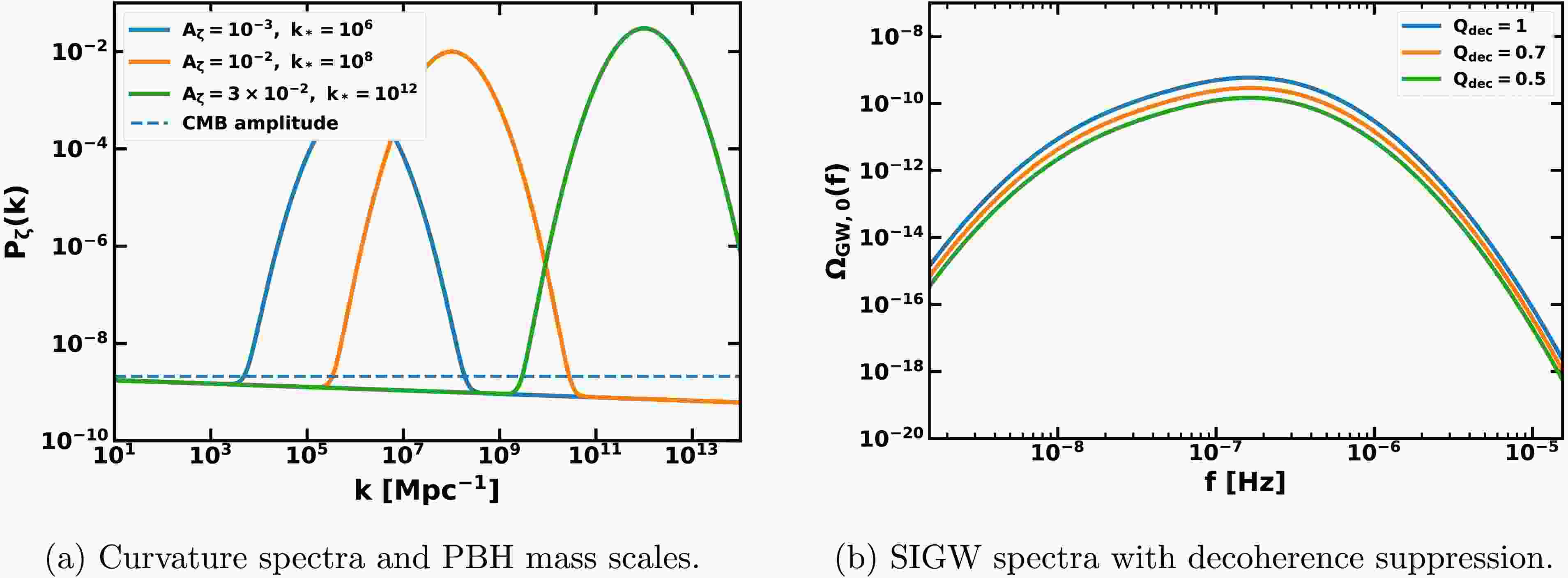
Before discussing the figures, we clarify the status of the primordial scalar spectrum used in the numerical analysis. The present study is deliberately inflation-model agnostic at the level of the microscopic inflaton potential. Our objective is to investigate how a primordial scalar covariance, once generated, is processed by a specified open-system channel and subsequently enters the PBH abundance and the scalar-induced gravitational-wave signal. The ultra-slow-roll discussion in Sec. II therefore provides a generic dynamical motivation for a localized enhancement of the small-scale curvature spectrum; it is not intended to identify a unique potential underlying Fig. 3(a).

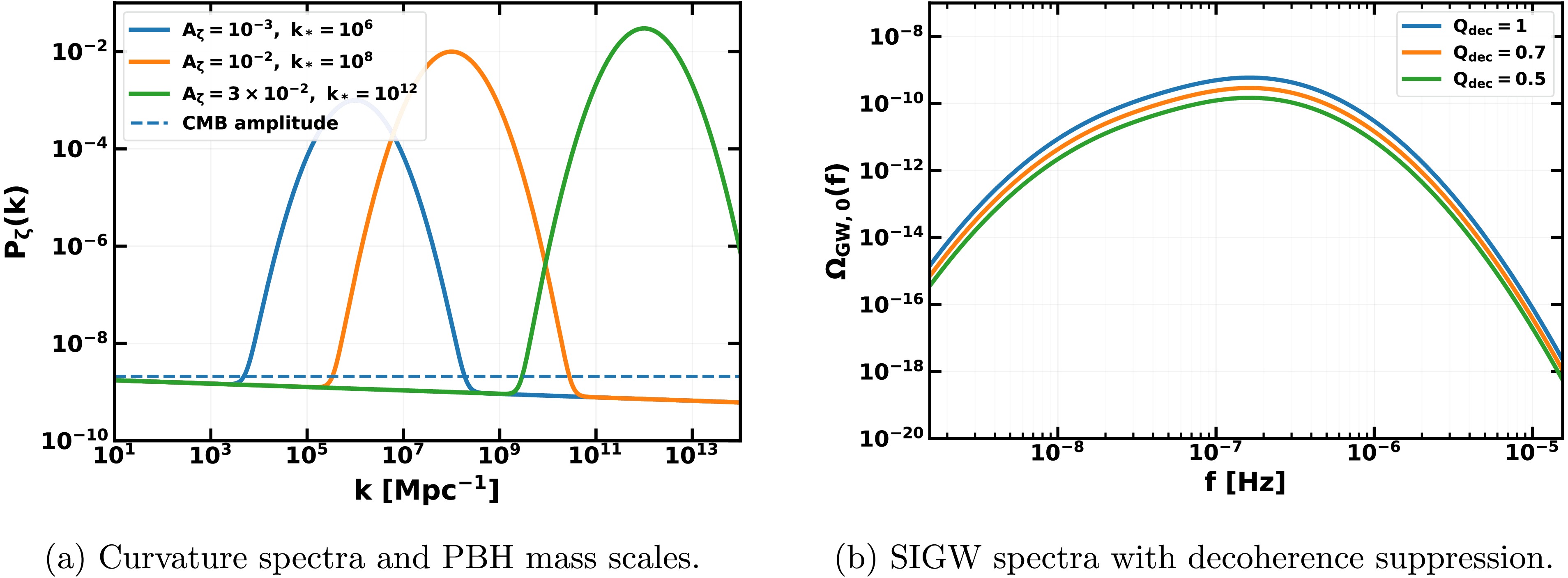
Figure 3.  (color online) Connection between the scalar spectrum, PBH formation, and scalar-induced gravitational waves. Panel (a) shows representative peaked curvature spectra. Changing the peak position shifts the corresponding PBH mass scale, whereas changing the amplitude controls the abundance through the classical collapse probability. Panel (b) shows a benchmark example of induced gravitational-wave spectra. In the constant-$ Q_{{\rm{dec}}} $ attenuation benchmark, covariance attenuation suppresses the amplitude by $ Q_{{\rm{dec}}}^2 $ without changing the spectral shape. A scale- or time-dependent attenuation factor instead leads to a frequency-dependent distortion.

Accordingly, we take the primordial spectrum itself as the input to the open-system calculation and use a generic lognormal benchmark. This lognormal parametrization is a standard and particularly useful benchmark for scalar-induced gravitational waves; see, e.g., Pi and Sasaki [62].

where $ A_\zeta $, $ k_* $, and $ \sigma_{\ln k} $ control, respectively, the amplitude, location, and logarithmic width of the small-scale enhancement. We use $ A_s=2.1\times10^{-9} $, $ k_0=0.05\, {{\rm{Mpc}}}^{-1} $, $ n_s=0.965 $, and the benchmark width $ \sigma_{\ln k}=1 $. The three curves in Fig. 3(a) correspond to $ (A_\zeta, k_*/{{\rm{Mpc}}}^{-1})= (10^{-3}, 10^6) $, $ (10^{-2}, 10^8) $, and $ (3\times10^{-2}, 10^{12}) $, respectively; the SIGW panel uses the middle benchmark. Figure 3(a) should therefore be interpreted as a set of representative primordial inputs rather than as the prediction of a specific inflationary potential.

This separation is useful because the open-system relations derived in this work can be applied without modification to any microscopic inflationary construction that produces a comparable $ {\cal{P}}_\zeta(k) $. A dedicated first-principles embedding would require specifying $ V(\phi) $ and solving the background and Mukhanov–Sasaki equations and, in the PBH regime, controlling the associated non-Gaussian statistics. Such explicit realizations, including supersymmetric and non-supersymmetric inflationary scenarios, are outside the scope of the present paper and constitute a natural direction for future work. We first examine the quantum state of the PBH-producing curvature modes, then trace the effect of decoherence on entanglement and discord, and finally connect the surviving scalar covariance to PBH abundance and scalar-induced gravitational waves. This ordering keeps the interpretation conservative: PBH formation remains a classical collapse process, while the quantum-information variables diagnose the state of the perturbations that seed the collapse and source the induced tensor background.

Figure 1 provides a reference point for the quantum-information part of the analysis. It shows the pure-state Gaussian discord as a function of the squeezing parameter r, using Eq. (46). The numerical crossings shown in the figure are consistent with Eqs. (47)–(50). The thresholds $ \mathcal D_G=0.2, 1.0 $, and 3.0 bits are reached at $ r=0.175, 0.519 $, and 1.232, respectively. The shaded region marks $ r>1 $, where the discord already exceeds about 2.34 bits. This provides an important baseline result. In the absence of decoherence, strong squeezing automatically implies large Gaussian discord. Therefore, a low discord threshold is not an independent PBH-formation condition. Instead, it serves as a diagnostic of the quantum correlations already present in the two-mode squeezed state. This interpretation is consistent with the standard squeezed-state description of inflationary perturbations and with the use of Gaussian discord as a measure of quantum correlations [30, 31, 34, 35, 37].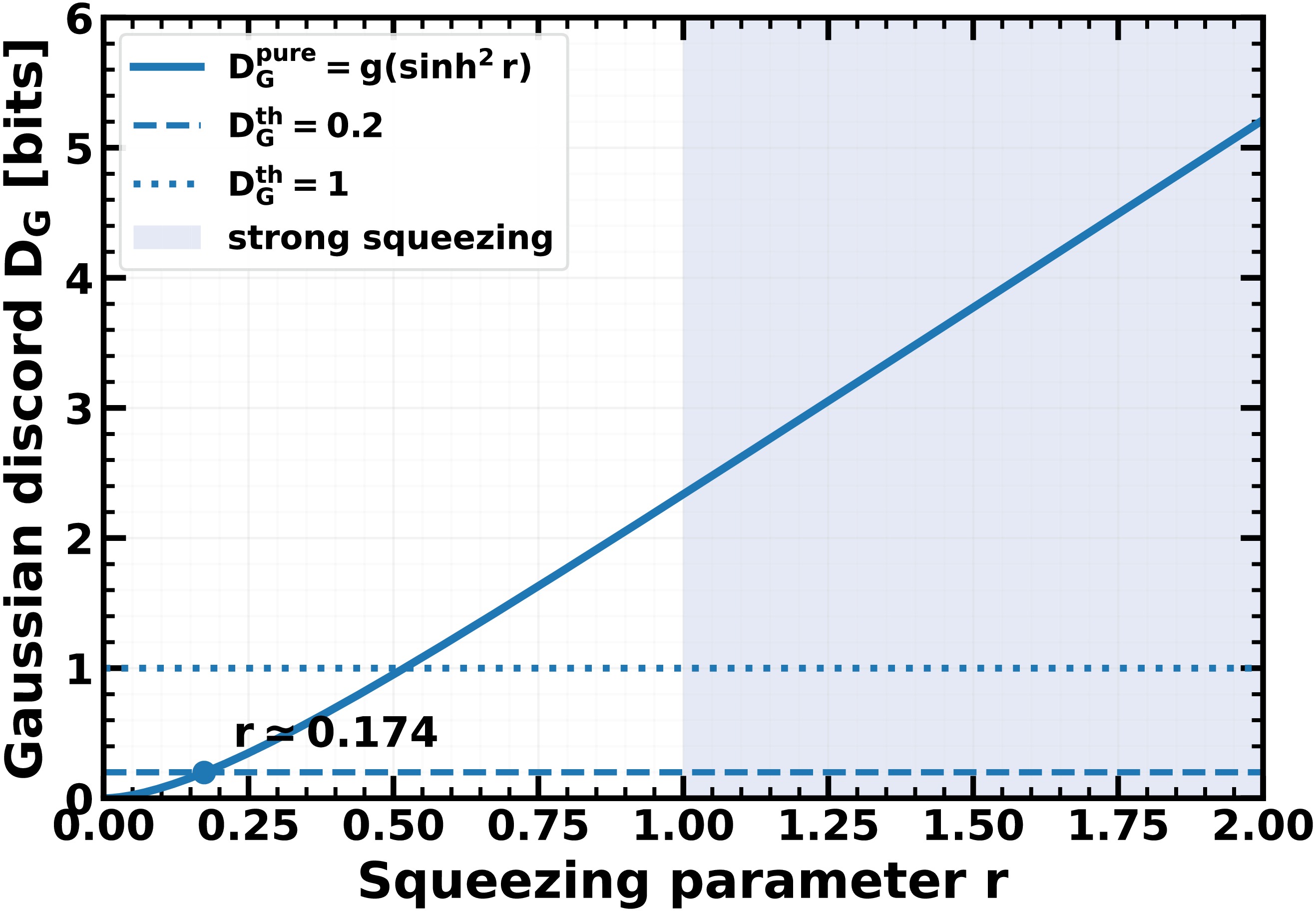

Figure 1.  (color online) Pure-state Gaussian discord as a function of the squeezing parameter r. The threshold values $ \mathcal D_G=0.2 $, 1.0, and 3.0 bits are reached at $ r=0.175 $, 0.519, and 1.232, respectively. The shaded region denotes the strongly squeezed regime, $ r>1 $, in which the pure-state discord is already large. The figure shows that strongly squeezed PBH-producing modes naturally exhibit large discord before decoherence is included.

The pure-state result is useful, but it does not correspond to the main physical regime of interest. The more informative case is the mixed state generated by environmental decoherence. Figure 2 illustrates this regime using the Gaussian attenuation channel described by Eqs. (69)–(71). The left panel of the figure shows the logarithmic negativity, computed from Eq. (80). As the channel transmissivity η is reduced, the state becomes increasingly mixed, and the logarithmic negativity can vanish at finite decoherence strength. This behavior reflects the familiar fragility of entanglement in an open quantum system.

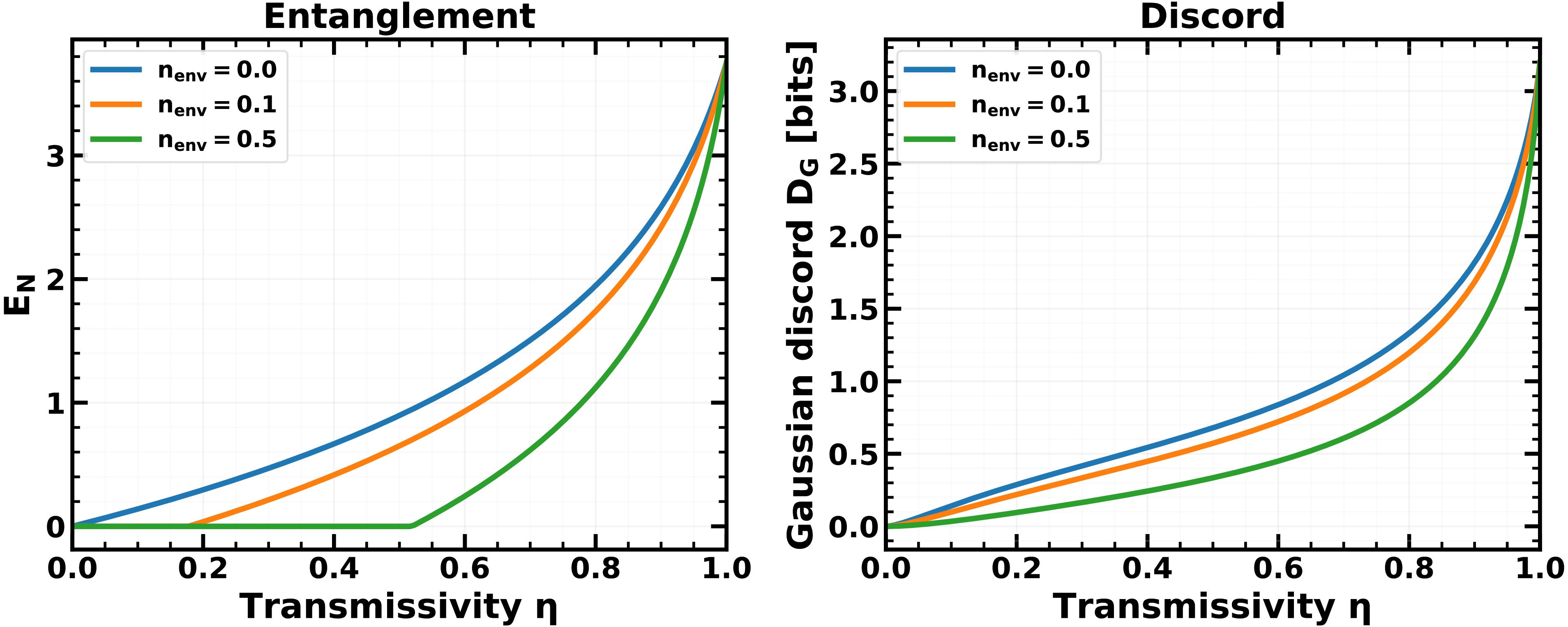
Figure 2.  (color online) Entanglement and Gaussian discord under the Gaussian decoherence channel. The logarithmic negativity $ E_N $ is rapidly degraded as the transmissivity η decreases and may vanish at a finite decoherence strength. Gaussian discord is more robust and may remain nonzero even after the state becomes separable. The figure therefore demonstrates why discord is a useful diagnostic of residual quantum correlations in the PBH-producing curvature modes.

The right panel of Fig. 2 shows the corresponding Gaussian discord, computed from Eq. (87). Although the discord also decreases as decoherence strengthens, it persists over a larger region of parameter space than the logarithmic negativity. The figure therefore distinguishes three physically distinct regimes: a nearly pure squeezed regime, a mixed entangled regime, and a separable but still discordant regime. The last regime is the most relevant for our purposes. It shows that the loss of entanglement does not by itself imply that the curvature perturbations have become a completely classical stochastic ensemble. A separable Gaussian state can still retain phase-space correlations inherited from the original inflationary squeezing [34−36].

We next connect these quantum-information diagnostics to the scalar sector that governs PBH formation and scalar-induced gravitational waves. The left panel of Fig. 3 shows representative peaked curvature spectra. Shifting the peak to larger $ k_* $ corresponds to perturbations that re-enter the Hubble radius earlier and hence to smaller PBH masses. Increasing the peak amplitude raises the smoothed density variance in Eq. (97). Since the classical PBH abundance depends on the tail of the distribution through Eq. (100) and becomes exponentially sensitive in the small-variance limit described by Eq. (101), even a modest change in the scalar amplitude can produce a large change in $ f_{{\rm{PBH}}} $. This is why the PBH abundance is a highly sensitive probe of the small-scale scalar spectrum [2, 8−10].

The same scalar spectra also source induced gravitational waves. The right panel of Fig. 3 shows the corresponding SIGW spectra. The standard result is determined by the convolution in Eq. (117). Once the scalar covariance is modified by a covariance-survival factor, the Gaussian static contribution is given by Eq. (127). This equation serves as a benchmark for the Wick-reduced attenuation model, rather than as a general formula for cosmological decoherence; a connected trispectrum contributes the term in Eq. (116). The simpler $ Q_{{\rm{dec}}}^2 $ scaling shown in the plot applies only in the narrow-peak and slowly varying $ Q_{{\rm{dec}}} $ limit, as stated in Eq. (129). Thus, for a constant benchmark $ Q_{{\rm{dec}}}=0.7 $, the induced signal is reduced by a factor of 0.49, while $ Q_{{\rm{dec}}}=0.5 $ yields a reduction by 0.25. The shape remains unchanged in this simple limit because the same constant factor multiplies the scalar covariance across the support of the convolution. By contrast, a scale-dependent or time-dependent decoherence history would distort the spectrum and would require the more general treatment discussed around Eq. (132).

The constant-$ Q_{{\rm{dec}}} $ curves in Figs. 3 and 4 must therefore be interpreted as response/sensitivity curves. Without an independent prediction for $ A_\zeta $, the pairs $ (A_\zeta, Q_{{\rm{dec}}}) $ and $ (A_\zeta Q_{{\rm{dec}}}, 1) $ are observationally indistinguishable at this level. The figures do not, by themselves, identify the suppression as quantum decoherence.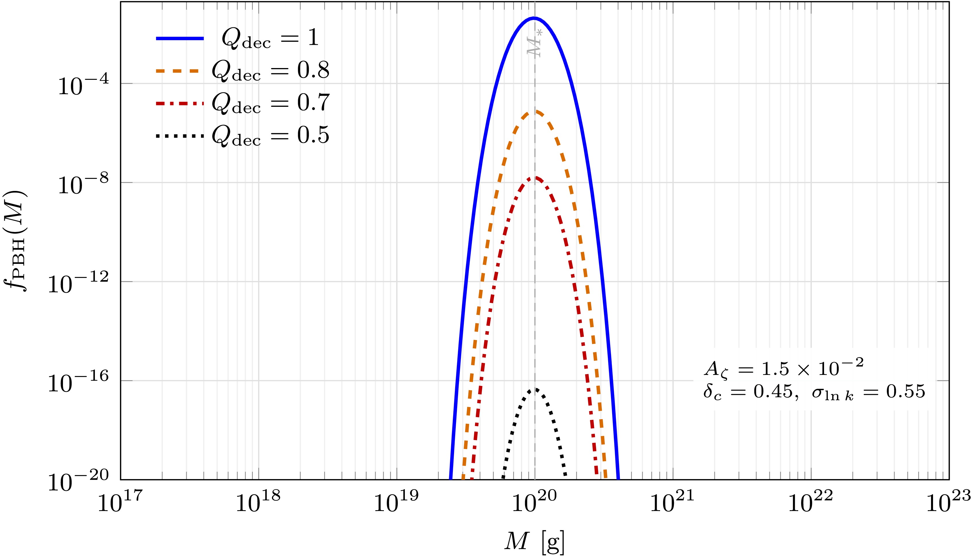

Figure 4.  (color online) Illustrative PBH dark-matter fraction as a function of PBH mass for constant covariance-survival factors $ Q_{{\rm{dec}}} $. The benchmark uses $ A_\zeta=1.5\times10^{-2} $, $ \sigma_{\ln k}=0.55 $, $ \delta_c=0.45 $, $ M_*=10^{20}\, {{\rm{g}}} $, $ \gamma=0.2 $, and $ g_*=106.75 $. The rapid separation of the curves demonstrates the exponential sensitivity of PBH production to the effective variance. Thus, the PBH abundance changes only when the open-system channel attenuates the scalar two-point covariance; pure dephasing with $ Q_{{\rm{dec}}}=1 $ leaves this abundance unchanged at the power-spectrum level.

To show explicitly how the covariance–survival factor affects the PBH abundance, we use Eqs. (110), (111), and (102) together with the mass–scale relation in Eq. (104). The illustrative calculation assumes a narrow lognormal curvature peak, using the same lognormal convention as in Ref. [62],

and a constant covariance–survival factor across the peak,

This approximation serves only as a benchmark. A complete prediction would require the model-dependent scalar spectrum, window function, transfer function, and possible non-Gaussian corrections. Nevertheless, it clearly illustrates the main effect: because $ \beta_f $ contains $ \exp[-\delta_c^2/(2\sigma_\delta^2)] $, a moderate reduction in the variance produces a much larger reduction in $ f_{{\rm{PBH}}} $.

Figure 4 shows that the PBH mass distribution retains approximately the same characteristic mass when $ Q_{{\rm{dec}}} $ is taken to be constant over the narrow peak, but its normalization is strongly suppressed. In the benchmark shown, reducing the scalar covariance from $ Q_{{\rm{dec}}}=1 $ to $ Q_{{\rm{dec}}}=0.8 $ already decreases the peak fraction by several orders of magnitude, and $ Q_{{\rm{dec}}}=0.7 $ suppresses it even further. This behavior is much stronger than the $ Q_{{\rm{dec}}}^2 $ scaling of the SIGW spectrum because PBH formation probes the extreme Gaussian tail, whereas the induced GW signal is quadratic in the scalar power spectrum.

To show explicitly how a scale-dependent survival factor modifies the full SIGW spectrum, we evaluate the microscopic family in Eq. (62).

Thus, all cases have $ Q_{{\rm{dec}}}(k_*)=0.7 $. We compare the cases $ \alpha=0, 1/2, 1 $. For the SIGW calculation, we use the middle spectrum in Fig. 3(a), with $ A_\zeta=10^{-2} $, $ k_*= 10^8\, {{\rm{Mpc}}}^{-1} $, $ \sigma_{\ln k}=1 $, and numerically evaluate the full u–v convolution using Eqs. (120) and (121). For the PBH comparison, we use the benchmark in Fig. 4, with $ A_\zeta=1.5\times10^{-2} $, $ \sigma_{\ln k}=0.55 $, $ \delta_c=0.45 $, and $ M_*=10^{20}\, {{\rm{g}}} $, together with the transparent narrow-peak horizon-entry estimate $ \sigma_\delta^2(M)\simeq(16/81){\cal{P}}^{{\rm{eff}}}_\zeta(k_M) $ and Eq. (102). The results are summarized in Table 1.

The peak quantities in Table 1 capture only part of the effect. To make the scale dependence explicit at the spectral level, we now substitute Eq. (145) directly into the full Gaussian SIGW convolution, Eq. (127), and plot the resulting present-day energy-density spectra. The calculation uses the same middle benchmark as Fig. 3(a), namely $ A_\zeta=10^{-2} $, $ k_*=10^8\, {{\rm{Mpc}}}^{-1} $, and $ \sigma_{\ln k}=1 $.

Figure 5 illustrates why, in general, the scale-dependent case cannot be represented by a single overall factor multiplying $ \Omega_{{\rm{GW}}} $. The factors $ Q_{{\rm{dec}}}(ku)Q_{{\rm{dec}}}(kv) $ weight different parts of the radiation-era convolution differently. Consequently, for $ \alpha>0 $, both the amplitude and the shape of the SIGW spectrum change, whereas $ \alpha=0 $ reproduces the constant-attenuation limit.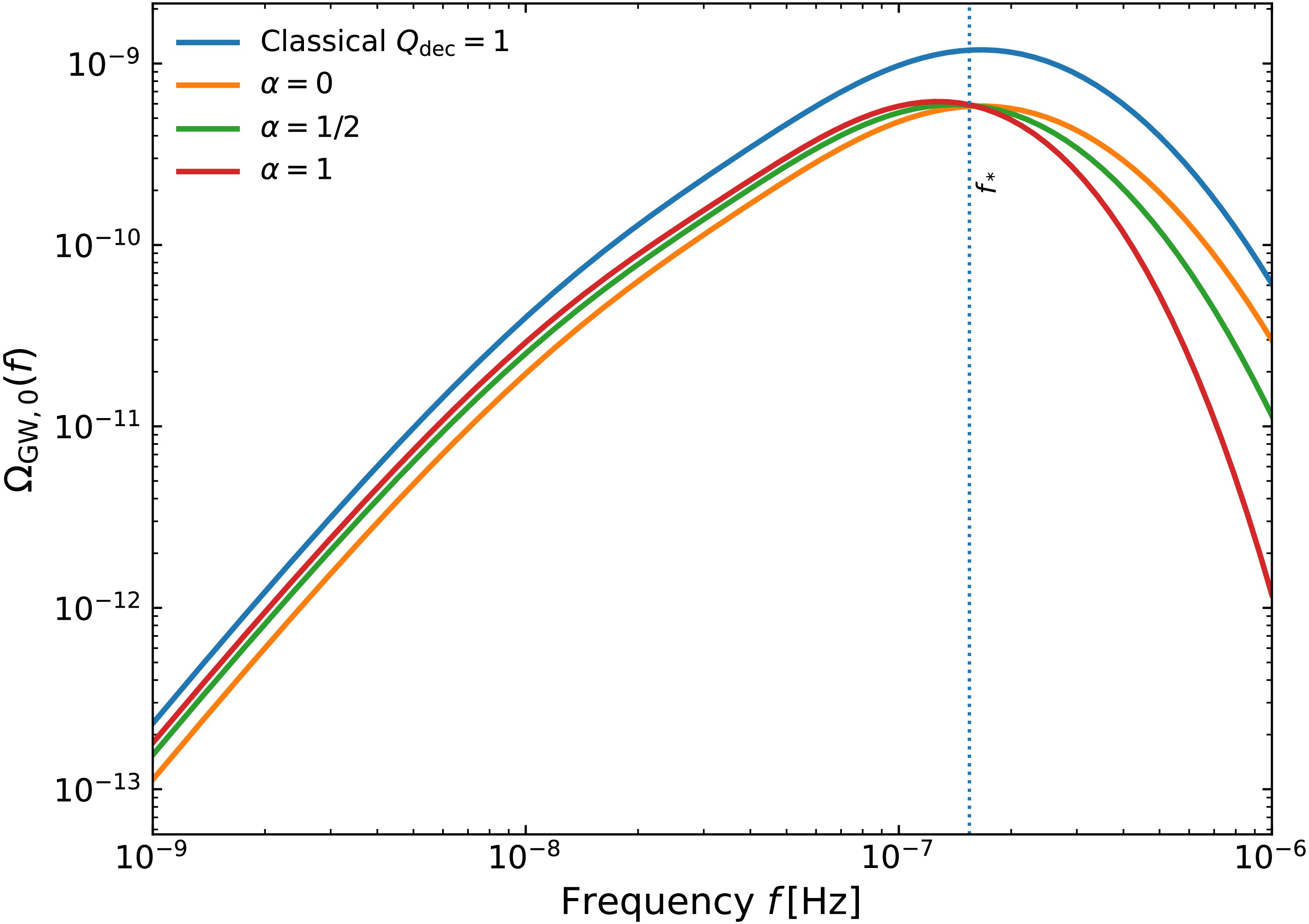

Figure 5.  (color online) Present-day scalar-induced gravitational-wave energy-density spectrum, obtained by inserting the scale-dependent survival factor $ Q_{{\rm{dec}}}^{(\alpha)}(k) $ of Eq. (145) into the full convolution in Eq. (127). The classical case, $ Q_{{\rm{dec}}}=1 $, is shown together with $ \alpha=0, 1/2, 1 $, all normalized to $ Q_{{\rm{dec}}}(k_*)=0.7 $. For $ \alpha=0 $, the spectral shape is unchanged, and the amplitude follows the constant-$ Q_{{\rm{dec}}} $ suppression. For $ \alpha>0 $, the stronger attenuation of higher-k scalar modes produces a frequency-dependent distortion and shifts the SIGW maximum toward lower frequencies.

For $ \alpha=0 $, the result reduces to the constant attenuation already shown in the figures: the SIGW peak is multiplied by $ 0.7^2=0.49 $, while the PBH abundance is affected much more strongly because of its exponential sensitivity to $ \sigma_\delta^{-2} $. For $ \alpha>0 $, shorter wavelengths are attenuated more strongly. Consequently, the PBH distribution is displaced toward larger masses ($ k_M\propto M^{-1/2} $), while the SIGW peak moves toward lower frequency. The fact that the peak SIGW amplitude is not exactly 0.49 of the classical value for $ \alpha>0 $ reflects the breakdown of the constant-$ Q_{{\rm{dec}}} $ approximation: different parts of the convolution are weighted by different values of $ Q_{{\rm{dec}}}(ku)Q_{{\rm{dec}}}(kv) $.

The complete set of figures should be read as a single chain of results. Figure 1 shows that the PBH-producing modes naturally acquire large pure-state discord once they are strongly squeezed. Figure 2 shows that the mixed-state problem is nontrivial: entanglement can be erased while discord remains nonzero. Figures 3 and 4 then show where the same covariance information enters cosmological observables. The PBH abundance is affected only if the open-system channel changes the classical scalar variance entering Eq. (110) and hence the effective collapse fraction in Eq. (111). By contrast, the SIGW signal is directly sensitive to the scalar covariance in Eq. (127). This is the main reason why induced gravitational waves provide a particularly clean probe of decoherence-suppressed scalar correlations.

The numerical examples therefore support a conservative interpretation. The standard PBH/SIGW calculation uses the scalar power spectrum, the classical collapse threshold, and the induced-GW kernel. The quantum-information extension retains the same collapse criterion, but tracks the full covariance matrix and distinguishes among pure squeezed, mixed entangled, and separable but discordant regimes. Finally, a specific dissipative decoherence model may introduce a covariance-survival factor $ Q_{{\rm{dec}}} $. This factor modifies the induced gravitational-wave spectrum according to Eq. (127) and reduces to the simple scaling in Eq. (129) only under the narrow-peak approximation. Its effect on PBH abundance is more model-dependent because PBH formation depends on the real-space density variance and the nonlinear collapse threshold. In this sense, quantum discord is not a new source of PBHs or gravitational waves. Rather, its value lies in tracking the quantum-to-classical transition of the scalar perturbations whose covariance later appears in PBH and SIGW observables.

We have studied how the decoherence of PBH-producing curvature perturbations can affect the primordial black-hole abundance and the associated scalar-induced gravitational-wave background. The PBH collapse criterion was kept classical: PBHs form when the density perturbation exceeds the threshold at horizon re-entry. Gaussian quantum discord was used only as a diagnostic of residual quantum correlations in the squeezed scalar modes, not as a new condition for PBH formation.

Using a Lindblad-inspired Gaussian loss channel, we separated two distinct effects. The first is the survival of quantum correlations, measured by Gaussian discord. The second is the possible suppression of the scalar two-point covariance, parameterized by $ Q_{{\rm{dec}}}(k) $. Only the second effect directly changes PBH and SIGW observables. For PBHs, it enters through the smoothed density variance and can strongly affect the abundance because the collapse probability is exponentially sensitive to this variance. For scalar-induced gravitational waves, the effect is more direct, because the induced tensor source is quadratic in the scalar perturbations. Therefore, in the narrow-peak limit and for slowly varying $ Q_{{\rm{dec}}} $, the spectrum scales approximately as $ Q_{{\rm{dec}}}^{2}\Omega_{{\rm{GW}}}^{{\rm{class}}} $.

The central result is that decoherence and residual quantum correlations can be incorporated into the standard PBH/SIGW framework without changing the classical collapse picture. In this formulation, Gaussian discord characterizes the quantum-to-classical transition of the scalar sector, while $ Q_{{\rm{dec}}} $ controls the observable effect at the covariance level. This provides a consistent way to relate the quantum history of PBH-producing perturbations to measurable signatures in scalar-induced gravitational waves.

We stress, however, that PBH and SIGW data alone do not identify decoherence: they constrain the effective scalar statistics. A constant $ Q_{{\rm{dec}}} $ is exactly degenerate with the primordial peak amplitude, and a scale-dependent $ Q_{{\rm{dec}}}(k) $ can be degenerate with the primordial spectral shape. The interpretation as attenuation becomes predictive only after a microscopic channel and independent information about its parameters or the unattenuated inflationary spectrum have been supplied. Moreover, our explicit SIGW formula gives the Gaussian/Wick-reduced contribution; significant USR non-Gaussianity or interaction-generated connected four-point functions must be included separately.

Within the explicit thermal-loss example, the survival factor is determined by the bath spectral density through $ Q_{{\rm{dec}}}(k)\simeq\exp[-2\pi J_*\Delta t(k/k_*)^\alpha] $ in the cold-bath limit. The scale-dependent calculation in Sec. VIII B shows quantitatively that such a channel can shift the PBH mass distribution and the SIGW peak frequency, in addition to changing their amplitudes. Gaussian discord remains a distinct diagnostic of the quantum state and is not directly measured by these classical observables.