


 Abstract
 HTML
HTML Reference
 Related
 PDF
PDF


HTML
-
The study of fermions in the presence of kinklike structures has been initiated long ago, in the pioneering work by Jackiw and Rebbi [1]. An important information that appears from the investigations is the phenomenon known as fermion number fractionalization, which is due to the topological nature of the background bosonic structure [2]. The model investigated in [1] is defined in (1, 1) spacetime dimensions, and describes a real scalar field that interacts with a fermion field via the Yukawa coupling. For more on kinks and related issues see for example Ref. [3].
The interest in the fermion number fractionalization goes beyond its mathematical identification since it presents peculiarities that can be physically realized in condensed matter situations, as shown in Refs. [4, 5]. The subject has been investigated by other authors, and here we quote Refs. [6-10] to illustrate this possibility. As is known, the effect of the fermion number fractionalization is directly related to the topological behavior of the bosonic structure arising from the bosonic portion of the model. However, in a recent work [10], another possibility is investigated, focusing attention on the geometric conformation of the topological structure that the bosonic portion of the model brings into play.
The geometrical aspects of the structure is of current interest, since experiments may now be carried out on miniaturized samples in constrained geometries, and the geometry may drastically change the conformational structure of the topological object, as experimentally verified for instance in Ref. [11]. The change in the conformational structure of the bosonic background may induce distinct physical properties on the fermion field, as was presented in [10] and is further shown in the present work.
There are many reasons to study the interaction of fermion fields with bosonic backgrounds since it may create or affect other interesting physical phenomena like the Casimir effect [12, 13], the Bose-Einstein condensation [14], and the localization of fermions in braneworld scenarios [15-18]. Another motivation is the current interest in the study of miniaturized samples of magnetic materials [11, 19-22], and the recent investigation [10]. With this in mind, we introduce three models of the type considered in [1] which support distinct bosonic backgrounds. In the models, the bosonic portion that generates the topological structures was studied before in Refs. [23-25], and we use them to describe how the fermion field behaves in such distinct backgrounds. For the sake of simplicity we consider the minimal coupling between the fermion and the kink, the Yukawa coupling, since the main idea is to capture, in a general way, how the fermion would perceive the change in the kink profile. In the context of fermion-soliton systems it is the most common interaction considered in literature.
To implement the investigation, we organize the work as follows: In Sec. 2 we introduce the general model and deal with some of its properties which are of direct interest for the present investigation. We review the case of a fermion field coupled to the sine-Gordon model in Sec. 3, since this is also of general interest to the current work. We study three new models, explicitly showing how the fermion bound states and energies are characterized in each case. In the first two models, the bosonic background structures are controlled by a real parameter and obey the parity symmetry, but they behave differently as the parameter increases from zero to unity, one excluding and the other including fermionic bound states in the system. The third model is different, and the bosonic structure does not obey the parity symmetry anymore, so all the fermion bound states are asymmetric functions. We end the work in Sec. 4, where we add some comments and conclusions.
-
We are interested in studying models described by the Lagrangian
$ \begin{eqnarray} {\mathcal L} =\displaystyle \frac{1}{2}{\partial }_{\mu }\phi {\partial }^{\mu }\phi -V(\phi )+\displaystyle \frac{1}{2}\bar{\psi }{\rm{i}}\rlap{/}{\partial }\psi -\phi \bar{\psi }\psi, \end{eqnarray} $
(1) which is similar to the model of Ref. [1]. We are dealing with a scalar field represented by ϕ = ϕ(x, t) and a Dirac field denoted by ψ = ψ(x, t), which interact via the Yukawa coupling that appears in the last term of the above expression. In the models considered here we define
$V\left( \phi \right)=W_{\phi }^{2}/2$ , where Wϕ is the derivative of some function W=W(ϕ) with respect to the field ϕ. W in supersymmetric models is called superpotential, although here we are using it as a mathematical tool to simplify the calculations. Also, we use$\hbar$ = 1 = c and consider dimensionless fields and spacetime coordinates.We consider the topological structure of the kinklike profile which arises from the bosonic Lagrangian
$ \begin{eqnarray}{ {\mathcal L} }_{{\rm{b}}}=\displaystyle \frac{1}{2}{\partial }_{\mu }\phi {\partial }^{\mu }\phi -\displaystyle \frac{1}{2}{W}_{\phi }^{2}, \end{eqnarray} $
(2) as background solutions to be considered in the fermionic Lagrangian
$ \begin{eqnarray}{ {\mathcal L} }_{{\rm{f}}}=\displaystyle \frac{1}{2}i\bar{\psi }\rlap{/}{\partial }\psi -\phi \bar{\psi }\psi .\end{eqnarray} $
(3) The procedure is as follows: we first deal with the bosonic model (2) to find the static kinklike structure that solves the corresponding equation of motion
$ \begin{eqnarray}{\phi }^{\prime\prime}-{W}_{\phi }{W}_{\phi \phi }=0, \end{eqnarray} $
(4) where the prime stands for the derivative with respect to the spatial coordinate x. As is well-known, in this case the solutions obey the first-order equation
$ \begin{eqnarray}{\phi }^{\prime}={W}_{\phi }, \end{eqnarray} $
(5) and so are stable against small fluctuations.
The equation of motion for the fermion field has the form
$ \begin{eqnarray}({\rm{i}}\rlap{/}{\partial }-2\phi )\psi =0.\end{eqnarray} $
(6) For convenience, we choose to describe the gamma matrices by the set (γ0, γ1, γ5) = (σ1, iσ3, σ2). Moreover, since the scalar field describes a static structure we write the spinor field as
$ \begin{eqnarray*}\psi (x, t)={{\rm{e}}}^{-{\rm{i}}Et}\left(\begin{array}{c}{\psi }^{(+)}(x)\\ {\psi }^{(-)}(x)\end{array}\right).\end{eqnarray*} $
This ansatz can be inserted in Eq. (6) which allows to rewrite the equation of motion for the Dirac field as
$ \begin{eqnarray}E{\psi }^{(\pm )}+\left(\pm \displaystyle \frac{{\rm{d}}}{{\rm{d}}x}-2\phi \right){\psi }^{(\mp )}=0, \end{eqnarray} $
(7) which is a system of equations involving the components of the spinor field ψ. We can use this system of equations to obtain two Schrödinger-like equations given by
$ \begin{eqnarray}\left(-\displaystyle \frac{{{\rm{d}}}^{2}}{{\rm{d}}{x}^{2}}+{U}_{\pm }(x)\right){\psi }^{(\mp )}={E}^{2}{\psi }^{(\mp )}, \end{eqnarray} $
(8) where U
$\pm $ (x)=$\pm $ 2dϕ/dx+4ϕ2, with ϕ=ϕ(x) being the static kinklike solution of the bosonic system. The decoupled Eqs. (8) are used to find the fermion bound energy spectrum. In general, the solutions of the decoupled second order equations are not necessarily the solutions of the coupled first order equations. Therefore, using the resulting fermion bound energy spectrum, one can employ the first order Eqs. (7) to find the correct bound states of the fermion system.We note that equations (8) have the form Q
$\mp $ Q$\pm $ ψ($\pm $ ) = E2ψ($\pm $ ), where Q$\pm $ =$\pm $ d/dx+2ϕ. In particular, we can find an expression for the ground state wave function by solving Q$\pm $ ψ($\pm $ )=0, and obtain$ \begin{eqnarray}{\psi }_{0}^{(\pm )}={c}_{\pm }{{\rm{e}}}^{\mp 2{\displaystyle \int }^{x}\phi ({x}^{\prime}){\rm{d}}{x}^{\prime}}, \end{eqnarray} $
(9) where c
$\pm $ are normalization constants; for regularity of the ground state one of them has to be zero. To find the massive bound states, one uses Eqs. (7) and (8). It can also be shown that the stability equation for the scalar field is$ \begin{eqnarray}\left(-\displaystyle \frac{{{\rm{d}}}^{2}}{{\rm{d}}{x}^{2}}+{\left. \displaystyle \frac{{{\rm{d}}}^{2}V}{{\rm{d}}{\phi }^{2}}\right|}_{\phi =\phi (x)}\right){\eta }_{n}(x)={\omega }_{n}^{2}{\eta }_{n}(x), \end{eqnarray} $
(10) To get this equation, we have set ϕ(x, t) = ϕ(x) + Σnηn(x)cos(ωnt). In this case the zero mode η0(x) of the scalar field is proportional to the derivative of the static solution itself, i.e, η0(x)
$\approx $ ϕ'(x), and the solution is classically or linearly stable. To see this explicitly, we recall that$ \begin{eqnarray}\displaystyle \frac{{{\rm{d}}}^{2}V}{{\rm{d}}{\phi }^{2}}={W}_{\phi \phi }^{2}+{W}_{\phi }{W}_{\phi \phi \phi }, \end{eqnarray} $
(11) which has to be calculated for the classical static solution ϕ = ϕ(x). Thus, one can rewrite the second-order differential operator in Eq. (10) as
$ \begin{eqnarray}-\displaystyle \frac{{{\rm{d}}}^{2}}{{\rm{d}}{x}^{2}}+\displaystyle \frac{{{\rm{d}}}^{2}V}{{\rm{d}}{\phi }^{2}}=\left(-\displaystyle \frac{{\rm{d}}}{{\rm{d}}x}-{W}_{\phi \phi }\right)\left(\displaystyle \frac{{\rm{d}}}{{\rm{d}}x}-{W}_{\phi \phi }\right), \end{eqnarray} $
(12) which can be defined as S†S. Multiplying Eq. (10) by η† from the left, using the Eq. (12) and integrating over the whole space we find
$ \begin{eqnarray}{\omega }^{2}=\displaystyle \frac{\displaystyle {\int }_{-\infty }^{-\infty }{\rm{d}}x\, |S\eta {|}^{2}}{\displaystyle {\int }_{-\infty }^{-\infty }{\rm{d}}x\, |\eta {|}^{2}}, \end{eqnarray} $
(13) which means that ω2 has non-negative eigenvalues.
Another interesting result is that the threshold energy is taken at the limit ϕ(x
$\to $ ) = ϕmin, where the bosonic field approaches the minimum of the scalar potential. Moreover, for the well-behaved solutions of the fermionic bound states we require that in this regime ψ($\pm $ )$\to $ c$\pm $ and dψ($\pm $ )/dx$\to $ 0. In this way, the threshold energy equation, derived from (7), becomes Ethc$\pm $ -2ϕminc$\mp $ =0, and thus one finds Eth=2ϕmin, which is equal to the square root of U$\pm $ for spatial infinities, as expected.
-
Let us now consider some explicit models. We are interested in studying the fermion field behavior when it evolves in the background of a kinklike structure derived from the bosonic model defined in terms of the potential
$ \begin{eqnarray}V(\phi )=\displaystyle \frac{1}{2}{W}_{\phi }^{2}, \end{eqnarray} $
(14) for the following three distinct cases:
$ \begin{eqnarray}{W}_{\phi }=\displaystyle \frac{1}{1-\lambda }{\rm{cd}}(\phi, \lambda ), \end{eqnarray} $
(15a) $ \begin{eqnarray}{W}_{\phi }=\displaystyle \frac{2{{\rm{cn}}}^{2}(\phi /2, \lambda )-(1-\lambda )}{{\rm{dn}}(\phi /2, \lambda )}, \end{eqnarray} $
(15b) and
$ \begin{eqnarray}{W}_{\phi }=(1-\phi )(1+{\phi }^{p}).\end{eqnarray} $
(16) Kinklike solutions for the bosonic models (15a) and (15b) were presented in [23, 24]. The models are written in terms of Jacobi's elliptic functions, where cd(ϕ, λ) = cn(ϕ, λ)/dn(ϕ, λ) and λ is a real parameter in the interval [0, 1]. Both (15a, 15b) reduce to the sine-Gordon model for λ
$\to $ 0, and approach solutions with infinite amplitude when λ$\to $ 1, but in quite different ways. Model (15a) has, for any value of λ, an infinite set of degenerate topological sectors with meson mass m2=1/(1-λ)2, which increases as λ$\to $ 1 and is not defined at λ = 1. Model (15b) has two different infinite sets of topological sectors, but the mass of the meson is m2=4(1-λ2), which decreases as λ$\to $ 1 and is well defined at λ = 1, where it is zero. For λ=0 these sets are equivalent, but they are different as we vary the λ parameter. In particular, the topological sector we choose to work on here approaches the vacuumless solution in the limit λ$\to $ 1.The third model is defined by Eq. (16). It was presented in [25], and the parameter p is an odd integer, p = 1, 3, 5,
$\ldots $ . Here the system presents a single topological sector, and the reflection symmetry is broken for p$\ne $ 1. In this case, there are no changes in the minima of the scalar potential, which are at ϕ=$\pm $ 1 for all p, so that the asymmetry is only revealed by the two classical meson masses, or by the potential seen by the fermion field.Considering the Lagrangian (3) for all three models, the system has energy-reflection symmetry given by γ1 as well as charge-conjugation symmetry which is representation dependent, and in the representation we have chosen is given by σ3. Therefore, we expect that the fermionic bound energy spectrum is symmetric around the E = 0 line in all cases considered here. However, although the first two models enjoy parity or reflection symmetry, the third model does not respect this symmetry, and so it should be studied more carefully.
Due to the relevance of the sine-Gordon model [26] in the context of the present work, let us first review its solution and stability. It appears as a particular case of the models (15a) and (15b) for λ = 0. Thus, we have Wϕ=cos(ϕ) and the solution for the scalar field has the form
$ \begin{eqnarray}\phi (x)=\pm {\sin }^{-1}(\tanh (x)).\end{eqnarray} $
(17) In this case, the stability potential associated with the bosonic field is given by VSG=1-2sech2(x), which has a reflectionless shape and only one bound state, the zero mode, given by η0 = sech(x). However, if we take the above solution and use it in equation (8), we end up with the following potentials
$ \begin{eqnarray}{U}_{\pm }=4{({\sin }^{-1}(\tanh (x)))}^{2}\pm 2{\rm{sech }}(x)\end{eqnarray} $
(18) which asymptotically approach U
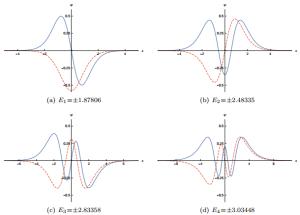
$\pm $ ($\pm $ ∞)=π2. The potential U_(x) allows nine fermionic bound states, which occur at the energies E0 = 0, E1 =$\pm $ 1.87806, E2 =$\pm $ 2.48335, E3 =$\pm $ 2.83358 and E4 =$\pm $ 3.03448. The zero mode can be obtained analytically and, up to a normalization factor, is given by$ \begin{eqnarray*}{\psi }_{0}(x, t)\propto \left(\begin{array}{c}{{\rm{e}}}^{-(2x(2{\cot }^{-1}({{\rm{e}}}^{x})+{\sin }^{-1}(\tanh (x)))+2{{\rm{Ti}}}_{2}({{\rm{e}}}^{-x}))}\\ 0\end{array}\right).\end{eqnarray*} $
Here, Ti2(x) is the inverse tangent integral, which can be written in terms of polylogarithmic functions by the relation Ti2(e-x)=i(Li2(-ie-x)-Li2(ie-x)). For the other bound states, we solve the set of equations in (7) and (8) and plot them in Fig. 1.
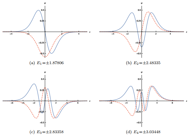
Figure 1. (color online) The ψ(+) (blue, solid line) and ψ(-) (red, dashed line) components of the massive bound states and the corresponding eigenenergies of the fermion field coupled to the sine-Gordon soliton (17).
-
Let us now look at model (15a) for general λ. In this case, the solution obtained for the scalar field is given by
$ \begin{eqnarray}\phi (x)={{\rm{sn}}}^{-1}\left(\tanh \left(\displaystyle \frac{x}{1-\lambda }\right), \lambda \right), \end{eqnarray} $
(19) where sn(x, λ) is the Jacobi elliptic sine, and its stability potential is
$ \begin{eqnarray}{\left.\displaystyle \frac{{{\rm{d}}}^{2}V}{{\rm{d}}{\phi }^{2}}\right|}_{\phi =\phi (x)}=\displaystyle \frac{1-\left(1-\displaystyle \frac{1}{1-\lambda }\cosh \left(\displaystyle \frac{2x}{1-\lambda }\right)\right){{\rm{sech }}}^{4}\left(\displaystyle \frac{x}{1-\lambda }\right)}{{\left(1-\lambda {\tanh }^{2}\left(\displaystyle \frac{x}{1-\lambda }\right)\right)}^{2}}.\end{eqnarray} $
(20) It approaches U(x
$\to $ $\pm $ ∞)∼1/(1-λ)2, which implies that the depth of the well increases with λ. For λ = 0 the expression (20) is well defined and has only one bound state which is the sine-Gordon case. However, for the other values of λ, we find an excited state, which has an energy gap with respect to the ground state that increases with λ.Given the Yukawa coupling between the boson and fermion fields, the Dirac field spectrum must be affected by changes in the behavior of the bosonic structure. For Model Ⅰ, the fermionic eigenstates are given by equations (7) and (8), and now the potentials U
$\pm $ have the form$ \begin{eqnarray}\begin{array}{lll}{U}_{\pm }&=&4{\left({{\rm{sn}}}^{-1}\left(\tanh \left(\displaystyle \frac{x}{1-\lambda }\right), \lambda \right)\right)}^{2}\\ &&\pm \displaystyle \frac{2}{1-\lambda }{\rm{cd}}\left({{\rm{sn}}}^{-1}\left(\tanh \left(\displaystyle \frac{x}{1-\lambda }\right), \lambda \right), \lambda \right).\end{array}\end{eqnarray} $
(21) The behavior of U_ is shown in Fig. 2. Asymptotically, it approaches U
$\pm $ ($\pm $ ∞)=4K(λ)2, where K(λ) is the complete elliptic integral of the first kind, which diverges as λ$\to $ 1. At x=0 one gets U$\pm $ (0)=$\pm $ 2/(1-λ). Therefore, for U_ the depth of the well increases but its width reduces as λ$\to $ 1. This effect is illustrated in Fig. 2, and it causes the exclusion of bound states in the well, as shown in Fig. 3, as expected from the quantum mechanical point of view. The issue here is that the bosonic structure becomes more localized as λ increases, and this contributes to the expulsion of the fermionic bound states. In particular, one can see that for the following values of λ there are different numbers of bound states: for λ=1/4, nine bound states; for λ=1/2, seven bound states; for λ=3/4, five bound states; and for λ=9/10, only one bound state. To find numerically the bound states in this model, and the other two as well, we solved the eigenvalue problem of Eq. (8) using Mathematica. Besides, we confirmed the results by solving the first order differential equations in (7) using the Runge-Kutta-Fehlberg method of order 5, which is a well known method to solve a set of coupled differential equations. The boundary condition we have used is that the value of the fermion bound states should be zero at infinities, which follows from the definition of the bound states. The results of the two calculations are indistinguishable within the numerical precision.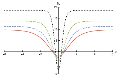
Figure 2. (color online) The U_ potential that appears in Eq. (21) for Model Ⅰ, shown for λ = 0, 0.25, 0.5, 0.75, depicted by solid, dashed, dot-dashed and dotted curves, respectively.
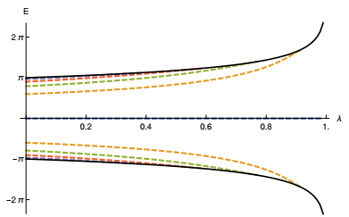
Figure 3. (color online) The fermionic bound state energy spectrum as a function of λ for Model Ⅰ. The solid (black) curves correspond to threshold energies.
Unfortunately, we could not find the analytical expression for the bound state wave functions corresponding to an arbitrary λ. Nevertheless, we could observe some characteristics of its behavior. In the vicinity of x=0 the scalar field behaves as
$\phi \left( {x \to 0} \right) \simeq x/\left( {1-\lambda } \right) + {\cal O}\left( {{x^3}} \right)$ , so the shape of the ground state in this region is$\simeq {{\rm{e}}^{-{x^2}}}^{/\left( {1-\lambda } \right) + {\cal O}\left( {{x^4}} \right)}$ , which means that higher the value of λ, the narrower is the wave function. Moreover, asymptotically the scalar field is ϕ(x$\to $ ∞)$\simeq $ e-x/(1-λ)+K(λ), which implies a decay proportional to e-2K(λ)x in the ground state wave fucntion as λ$\to $ 1. The behavior of the fermionic zero mode wave function in these two limits suggests that as λ increases, the normalized wave function becomes taller and narrower, as illustrated in Fig. 4. The same effect occurs for the excited states of the model.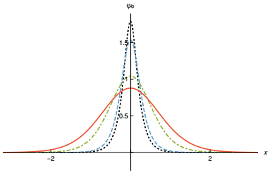
Figure 4. (color online) The normalized fermion zero mode in Model Ⅰ derived from equations (7) and (8) with the scalar field given by (19); λ = 0, 0.5, 0.9, 0.95, depicted by solid, dashed, dot-dashed and dotted curves, respectively.
-
We now study model (15b) for general λ. As shown in [24], this model has two solutions. In one of them there is a transition between the sine-Gordon kink and the vacuumless solution presented in [27, 28] so we choose this solution as the background field. It is given by
$ \begin{eqnarray}\phi (x)=2{{\rm{sc}}}^{-1}\left(\sqrt{\displaystyle \frac{1+\lambda }{1-\lambda }}\tanh \left(\displaystyle \frac{1}{2}\sqrt{1-{\lambda }^{2}}x\right), \lambda \right), \end{eqnarray} $
(22) where sc(ϕ, λ)=sn(ϕ, λ)/cn(ϕ, λ). Here, we have λ
$\in $ [0, 1], and the stability potential for the scalar field, which has only one bound state for any λ, evolves from a reflectionless shaped potential for the sine-Gordon case, to a volcano potential for the vacuumless solution. The drastic change in the shape of the stability potential can be explained by the behavior of the mass of the meson in the bosonic term of the Lagrangian (1), which approaches zero as λ$\to $ 1.Once we have chosen the solution (22) as the background field, we can look for the potential U_(x)
$ \begin{eqnarray}\begin{array}{lll}{U}_{-}&=&16{\left({{\rm{sc}}}^{-1}\left(\sqrt{\displaystyle \frac{1+\lambda }{1-\lambda }}\tanh \left(\displaystyle \frac{1}{2}\sqrt{1-{\lambda }^{2}}x\right), \lambda \right)\right)}^{2}\\ &&-\displaystyle \frac{2(1-{\lambda }^{2}){\rm{nd}}\left({{\rm{sc}}}^{-1}\left(\sqrt{\displaystyle \frac{1+\lambda }{1-\lambda }}\tanh \left(\displaystyle \frac{1}{2}\sqrt{1-{\lambda }^{2}}x\right), \lambda \right), \lambda \right)}{\cosh (\sqrt{1-{\lambda }^{2}}x)-\lambda }, \end{array}\end{eqnarray} $
(23) where nd(x, λ)=1/dn(x, λ). This potential is shown in Fig. 5. Unlike the previous model, we now have a system in which the number of bound states increases with λ; we are “capturing” more and more bound states as λ increases. This is illustrated in Fig. 6. In particular, when λ=1 and the fermionic potential becomes
$ \begin{eqnarray}{{U}_{\pm }|}_{\lambda =1}=16{\sinh }^{-1}{(x)}^{2}\pm \displaystyle \frac{4}{\sqrt{{x}^{2}+1}}\end{eqnarray} $
(24) 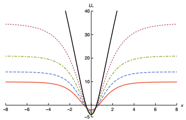
Figure 5. (color online) The U_ potential that appears in (23) for Model Ⅱ, shown for λ = 0, 0.25, 0.5, 0.75, and 1, depicted by solid (red), dashed, dot-dashed, dotted and solid (black) curves, respectively.

Figure 6. (color online) The fermionic bound state energy spectrum as a function of λ for Model Ⅱ. The solid curves correspond to threshold energies.
we find an infinite tower of bound states. The issue here is that the bosonic structure becomes less localized as λ increases, and this contributes to the inclusion of the fermionic bound states.
As in Model Ⅰ, we could not find analytically the zero energy solution for the Dirac field for general λ, but we could still get some information about its behavior. In the neighborhood of x = 0, the scalar field behaves as
$\phi \left( {x \simeq 0} \right) \simeq \left( {1 + \lambda } \right)x + {\cal O}\left( {{x^2}} \right)$ , so the wave function has the form${{\rm{e}}^{-\left( {1 + \lambda } \right){x^2} + {\cal O}\left( {{x^3}} \right)}}$ . However, we should be careful when analyzing its asymptotic behavior because of the fact that the form of the solution in this regime is$\phi \left( {x \to \infty } \right) \simeq {{\rm{e}}^{-\sqrt {1-{\lambda ^2}} x}} + {\phi _\infty }$ with${\phi _\infty } = 2{\rm{s}}{{\rm{c}}^{-1}}\left( {\sqrt {\frac{{1 + \lambda }}{{1-\lambda }}}, \lambda } \right)$ , which does not allow to study the particular case λ=1. However, a direct analysis of the vacuumless solution shows that the asymptotic behavior of the scalar field is in the form ϕλ=1(x$\to $ ∞)$\simeq $ -2lnx. Thus, the ground state wave function decays as e-2ϕ∞x for λ$\ne $ 1, and it decays as e4xx-4x for λ=1. We can integrate the vacuumless solution in order to find the exact form of the ground state at λ=1, which is$ \begin{eqnarray*}\psi (x, t)={c}_{+}\left(\begin{array}{c}{{\rm{e}}}^{-4(x{\sinh }^{-1}(x)-\sqrt{{x}^{2}+1})}\\ 0\end{array}\right).\end{eqnarray*} $
The normalized zero mode is displayed for representative values of λ in Fig. 7. We note that it remains well behaved in the full interval λ
$\in $ [0, 1], including λ=1, although there is an increase in its height. This behavior is different from the one shown in the previous section, since there the zero mode shrinks to a narrower and narrower region around its core x$\approx $ 0 as λ approaches unity.
Figure 7. (color online) The normalized fermion zero mode in Model Ⅱ derived from the solution (22) for λ = 0, 0.25, 0.5, 0.75, and 1, depicted by solid (orange), dot-dashed, dashed, dotted and solid (black) curves, respectively.
-
We now study how asymmetries within the scalar potential can affect the behavior of the fermionic bound states. We perform the numerical analysis of model (16), presented in [25]. This model presents a topological sector between ϕ = 1 and ϕ = -1, where the masses of the mesons are given by 4 and by 4p2, respectively. Note that as the scalar field asymptotically approaches ϕ(x
$\to $ $\pm $ ∞)$\to $ $\pm $ 1, the height and width of the well remain almost the same for all p, unlike what happens with the stability potential for the bosonic field. Thus, the difference between the masses of the mesons in the scalar potential generated by the variations of the parameter p implies only internal asymmetries in the fermion potentials, as shown in Fig. 8. Note that as the parameter p increases, the fermionic potential presents higher and higher asymmetry, and breaks the reflection symmetry; for negative values of x the potential reaches its maximum faster as p increases. This is in contrast with the behavior for positive x, which is smoother.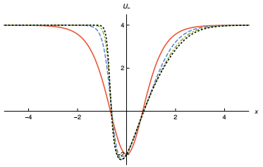
Figure 8. (color online) The U_ potential of Model Ⅲ, shown for p=1, 3, 5, and 7, depicted by solid, dashed, dot-dashed and dotted curves, respectively.
In Fig. 9, we show the fermion bound energy spectrum for several values of the parameter p. As one can see, the energy is not very sensitive to the value of p, although it is not entirely independent of p. In this model there are exactly three fermion bound energy states. The normalized fermionic zero mode is shown in Fig. 10, where we observe that the shape varies only slightly as p increases. This happens because asymptotically we have ϕ(x
$\simeq $ ∞)$\simeq $ 1-e-2x and ϕ(x$\simeq $ -∞)$\simeq $ -1+e2px, which implies that in the regime x$\simeq $ ∞ the ground state wavefunction decays as$\simeq $ e-2x-e-2x and in the limit x$\simeq $ -∞ it falls off as$\simeq {{\rm{e}}^{2x + \frac{1}{p}{{\rm{e}}^{2px}}}}$ . Consequently, for p > 1, the emerging nonlinearities due to the variations of this parameter are stronger for x < 0. Moreover, the asymmetry of the fermionic ground state evolves as a function of p more slowly than the bosonic zero mode asymmetry, presented in [25]. This is due to the fact that the field nonlinearities appear in the exponent of the exponential, and thus the changes of the curve shape are less pronounced. Therefore, in this model the fermionic zero mode responds asymmetrically to the parity-symmetry breaking.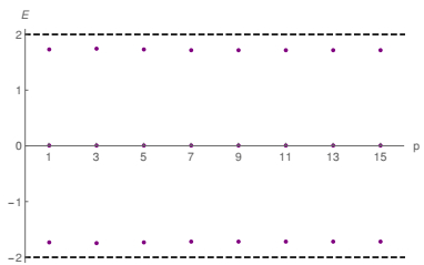
Figure 9. (color online) The fermion bound energy spectrum as a function of p in Model Ⅲ. The dashed lines correspond to threshold energies.

Figure 10. (color online) The normalized fermion zero mode derived from Model Ⅲ, shown for p=1, 3 and 5, depicted by solid (orange), dashed (blue) and dotted (black) curves, respectively.
In Fig. 11, we show the fermion massive bound states for the cases p=1 and p=3. One can see that the components ψ(+) and ψ(-) respect the parity symmetry for p=1, but this is not true anymore for the case p=3, as expected.
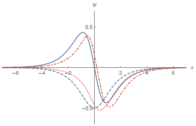
Figure 11. (color online) The ψ(+) and ψ(-) components of the massive bound states in Model Ⅲ, shown for p=1 with solid and dashed blue curves, and for p=3 with dot-dashed and dotted orange curves, respectively.
The asymmetry of the normalized zero mode shown in Fig. 10 can be quantified via the mean value
$ \begin{eqnarray}\mu =\displaystyle {\int }_{-\infty }^{\infty }{\rm{d}}xx{\psi }_{0}^{2}.\end{eqnarray} $
(25) The results are shown in Fig. 12, where one sees that there is no asymmetry for p=1; it appears for p=3, 5,
$\ldots $ and varies smoothly as p increases.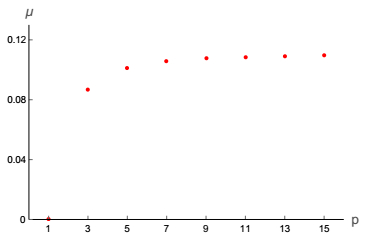
Figure 12. (color online) The mean value μ which measures the spatial asymmetry of the normalized zero mode, shown for several values of p.
3.1. Model Ⅰ
3.2. Model Ⅱ
3.3. Model Ⅲ
-
In this work we studied the behavior of the fermion field in the background of three kinklike structures that respond with distinct geometric conformations. The three bosonic structures arise from models described by a single real scalar field recently investigated with distinct motivations, but here we use them to see how the fermion bound energies and states behave in each case. The first two models are controlled by a real parameter, λ, which highlights fascinating characteristics of the models. The third model is different and is controlled by an odd integer parameter, p, which induces the parity-symmetry breaking, due to the asymmetric form of the bosonic potential.
Model Ⅰ has the peculiarity of describing a background potential for the fermion field, which deepens and narrows as λ approaches unity, such that the presence of the fermion bound states is reduced when λ increases. Model Ⅱ has a distinct behavior, and the background potential is now capable of adding new fermion bound states as the parameter λ increases in the interval [0, 1]. We find that as λ increases from zero to unity, the number of fermion bound states diminishes in Model Ⅰ, while it increases without limit in Model Ⅱ.
While Models Ⅰ and Ⅱ obey parity symmetry, Model Ⅲ engenders another behavior, which is also of current interest. It is controlled by an odd integer p=1, 3, 5,
$\ldots $ , capable of inducing the parity-symmetry breaking. The calculations are more intricate, but we have been able to show that the asymmetry present in the bosonic background is also induced in the potential of the fermion field, making the zero mode and the other bound states asymmetric. The asymmetry appears in the background potential and in the fermion bound states, and may be of practical use when one deals with asymmetric background structures; see for example Ref. [29], where the asymmetry of the localized structure plays a crucial role for understanding of the kink-antikink collisions in the ϕ6 model, and also Ref. [30] for the case of asymmetric structures in magnetic materials.


 DownLoad: