


 Abstract
 HTML
HTML Reference
 Related
 PDF
PDF


-
The discovery of neutrino oscillations [1-5], confirming the existence of the massive neutrinos, additionally motivates the search for new physics beyond the SM. Along with the neutrino mass puzzle, it is crucial to explore the nature of the neutrino. If neutrinos are Dirac particles, lepton number is conserved. Otherwise, lepton number violating (LNV) processes, which are forbidden in the SM, can be induced via Majorana neutrino exchange. Therefore, the LNV process is a promising signal for new physics beyond the SM. The aim of this paper is to study the B meson rare decays
$B^{+} \to K^{(*)+}\mu^+\mu^-$ in the SM and its extensions, and then to investigate the LNV process$B^{+}\to K^{(*)-}\mu^{+}\mu^+$ .Many experimental studies have been made in search of Majorana neutrinos by
$\Delta L=2$ processes, such as the most promising neutrinoless nuclear double beta decays ($0\nu\beta\beta$ ) [6, 7], LNV$\tau$ decays [8, 9], and$\Delta L=2$ $B, D, D_s, K$ meson decays [10-12]. With the upper limits given by the experiments, the bounds on the mass of neutrinos and the mixing matrix elements between neutrino and charged leptons have been investigated, which can serve to constrain the parameter space of new physics models. For the purpose of proving the Majorana nature of neutrinos,$0\nu\beta\beta$ as well as$\tau^- \to \ell^+ M_1^- M_2^-$ [13, 14],$\tau^- \to \pi^+ \mu^- \mu^- \nu_\tau$ [14, 15], and especially many same-sign charged dilepton$B, B_c, B_s, D, D_s, K$ meson decays have been widely investigated theoretically, including three-body LNV meson decays$B^+(B_c^+)\to \pi^-(K^{(*)-}, \rho^-, D^{(*)-}, D_s^{(*)-}) \ell^+ $ $\ell^{\prime +} ~(\ell^{(\prime)}\!=\!e, \mu) $ ,$D^+(D_{s}^+)\to \pi^- (K^{(*)-}, \rho^-) \ell^+\ell^{\prime +},K^+\to\pi^- \ell^+\ell^{\prime +}$ [13, 16-23], and four-body LNV meson decays$ \bar{B}^0 \to\pi^+(K^{(*)+}, \rho^+, D_{(s)}^+)$ $ D^+ \ell^-\ell^-$ ,$B^- \to \pi^+ (K^{(*)+}, \rho^+, D_{(s)}^+) D^0 \mu^-\mu^-$ ,$\bar{D}^0 \to \pi^+(K^+)$ $ \pi^+ \mu^-\mu^-$ ,$B_c^- \to J/\psi \pi^+ \mu^-\mu^-$ ,$B_c^- \to \bar{B}_s^0 \pi^+ \ell^-\ell^{\prime -}$ ,$B_s^0\to K^- (D_s^-) $ $\pi^- \mu^+\mu^+ $ [23-29]. Using the precision measurements of meson decays, the properties of Majorana neutrinos have been studied focusing on the masses and mixing matrix elements.Among various new physics models, Type-I seesaw mechanism is one of the most natural ways to generate tiny neutrino masses. In this model, the right-handed
${{S\!U}}{(2)_{\rm{L}}} \times {{U}}{(1)_{\rm{Y}}}$ singlet neutrinos$N_R$ are introduced to extend the SM. Apart from Dirac mass$M_D$ , the right-handed neutrino singlets with Majorana mass matrix$M_R$ are allowed with the gauge invariance. As a result, the effective mass matrix for the light neutrinos can be expressed with the canonical seesaw formula$M_{\nu}\sim$ $-M_{D}M_{R}^{-1}M_{D}^{T} $ . In terms of the neutrino mass eigenstate, the gauge interaction for the charged current is$ \begin{split} - {\cal L} =& \displaystyle\frac{g}{{\sqrt 2 }}W_\mu ^ + \left(\displaystyle\sum\limits_{\ell = e}^\tau {\displaystyle\sum\limits_{m = 1}^3 {U_{\ell m}^*} } \overline {{\nu _m}} {\gamma ^{\,\mu} }{P_L}\ell \right.\\ & +\left. \displaystyle\sum\limits_{\ell = e}^\tau {\displaystyle\sum\limits_{m' = 4}^{3 + n} {V_{\ell {m^\prime }}^*} } \overline {N_{{m^\prime }}^c} {\gamma ^{\,\mu} }{P_L}\ell \right) + h.c., \end{split} $

(1) where
$P_{L}=(1-\gamma_{5})/2$ ,$\nu_{m}(m=1, 2, 3)$ and$ N_{m^{\prime}}(m^{\prime}=4, \cdots,$ $ 3+n)$ are the mass eigenstates, and$U_{\ell m}$ ($V_{\ell m^{\prime}}$ ) is the mixing matrix element between the lepton flavor and light (heavy) neutrinos. Moreover, a number of proposals have been made to search for heavier Majorana neutrinos in$e^- e^-$ ($e^+ e^-$ ),$e\gamma$ ,$pp$ ($p\bar{p}$ ) collider experiments [30-34], and also in top quark and W boson rare decays [24, 35, 36].Majorana neutrino mass terms are well motivated by the so-called “see-saw” mechanism, in which the SM neutrino masses are tiny with a large mass scale suppression. Examples include Left-Right symmetric models, SO(10) supersymmetric models, grand unified models and extra dimension models. With a large mass scale in these models, the mass of the Majorana neutrino is generally heavy (up to TeV or larger). This kind of heavy neutrino could show rich phenomena at the hadron colliders [18, 37-40]. From the viewpoint of cosmology and astrophysics, a neutrino in the keV-GeV mass region could be a good candidate for dark matter, as well as for baryogenesis [41, 42]. Thus, Majorana neutrinos could have a wide mass range, from eV-TeV, which can be studied with hadron collisions, astronomical observations, neutrino experiments, nuclear decays, rare meson decays, etc. The B-meson rare decays could be sensitive to Majorana neutrino if its mass is a few GeV and the decay channels are kinematically allowed, especially in the
$B \to K$ semileptonic decays with resonances if$m_K<m_N<m_B$ .Semileptonic B meson decays
$B \to K^{(*)} \ell^+\ell^-$ induced by flavor changing neutral current are promising processes to test the SM and search for its extension. Precision measurements of the B meson decays have been performed by the CDF, BaBar and LHCb collaborations. Recently, the differential branching ratios of$B^{+}\to K^{+}\mu^+\mu^-$ and$B^{+}\to K^{*+}\mu^+\mu^-$ decays have been reported by the LHCb collaboration with the integrated luminosity of 3 fb−1, and the integrated branching fractions were found to be$(4.29\pm0.07 ({\rm stat}) \pm0.21({\rm syst}) ) \times10^{-7}$ and$(9.24\pm0.93 ({\rm stat}) \pm$ $0.67({\rm syst}) ) \times10^{-7}$ [43], respectively. This is the most precise measurement so far. Along with the development of the experiments, theoretical studies of$B \to K^{(*)} \ell^+\ell^-$ have been reported both in the SM [44-50] and new physics models [51-54]. The SM predictions for the branching ratios are comparable with the LHCb data, but new physics contributions can not be excluded. In this paper, we first study the opposite-sign B meson dileptonic rare decays$B^+ \to K^{(*)+} \mu^+\mu^-$ both in the SM and Type-I seesaw model. The contributions from Majorana neutrino are then investigated in the same-sign LNV process$B^+ \to K^{(*)-} \mu^+\mu^+$ .The paper is organized as follows. In Section 2, the theoretical framework is introduced with the formulas for B meson rare decays
$B^{+}\to K^{(*)+}\ell^{+}\ell^{-}$ in the SM and mediated by a Majorana neutrino, as well as the same-sign LNV decays$B^{+}\to K^{(*)-}\ell^{+}\ell^{+}$ . In Section 3, we give numerical results for the branching ratios, the dilepton invariant mass distributions and angular distributions of$B^{+}\to K^{(*)\pm}\mu^{+}\mu^{\mp}$ . The excluded regions of Majorana neutrino mass and mixing matrix element are given by the fit results. Furthermore, the dilepton invariant mass distributions and the dilepton angular distributions of LNV processes are studied. Finally, we give a brief summary. -
We first study the B meson rare decays
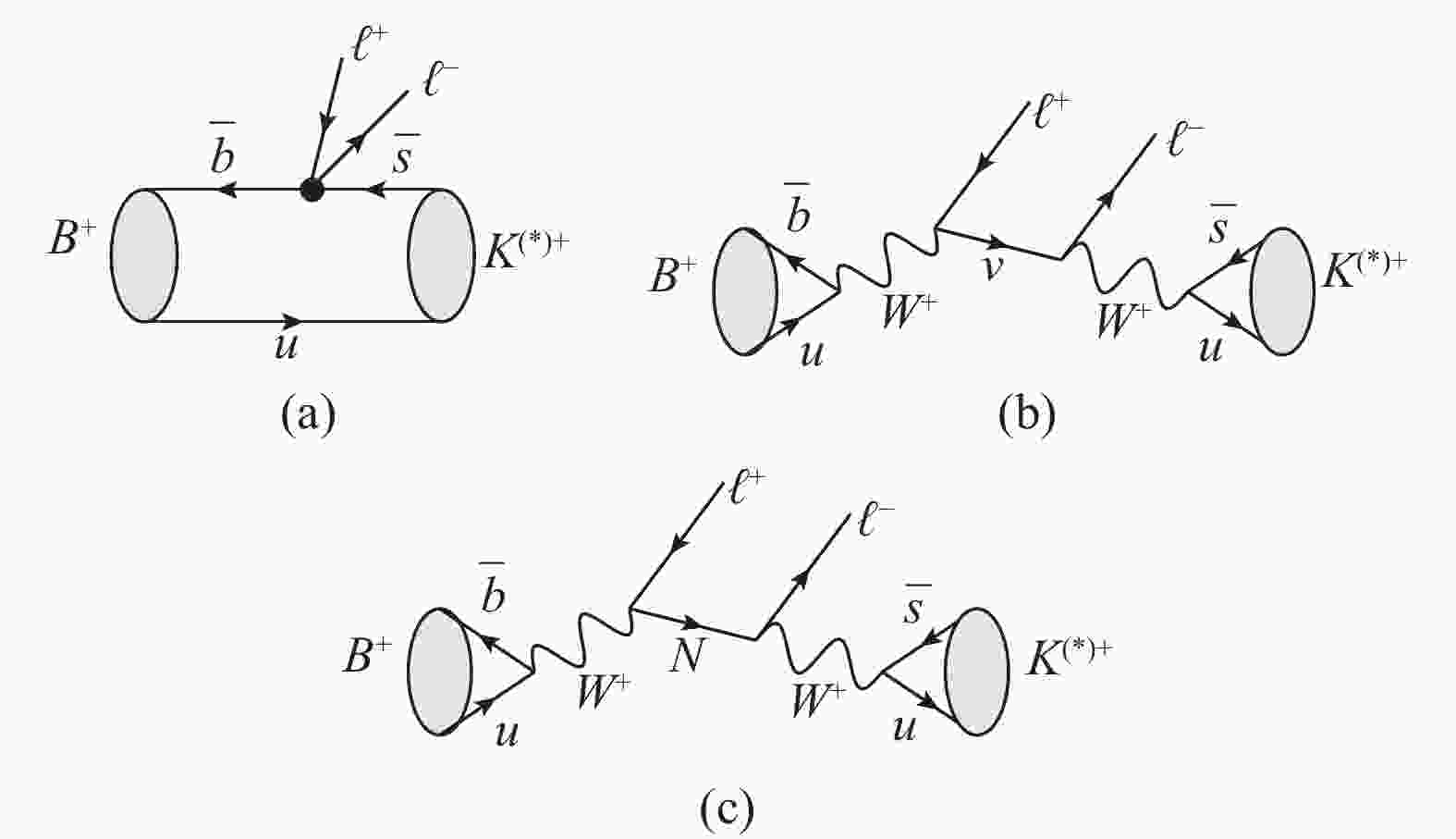
$ B^{+}(p_B)\to K^{(*)+}$ $ (p_{K^{(*)}}) \ell^{+}(p_1) \ell^{-}(p_2)$ . Fig. 1(a) is the Feynman diagram for$B^{+}\to K^{(*)+}\ell^{+}\ell^{-}$ in the SM. These processes are induced by the flavor changing neutral current$\bar{b}\to \bar{s}\ell^+\ell^-$ , which can be described through the effective Hamiltonian [5]. The decay amplitude of$\bar{b}\to \bar{s}\ell^+\ell^-$ can be written as [45, 55]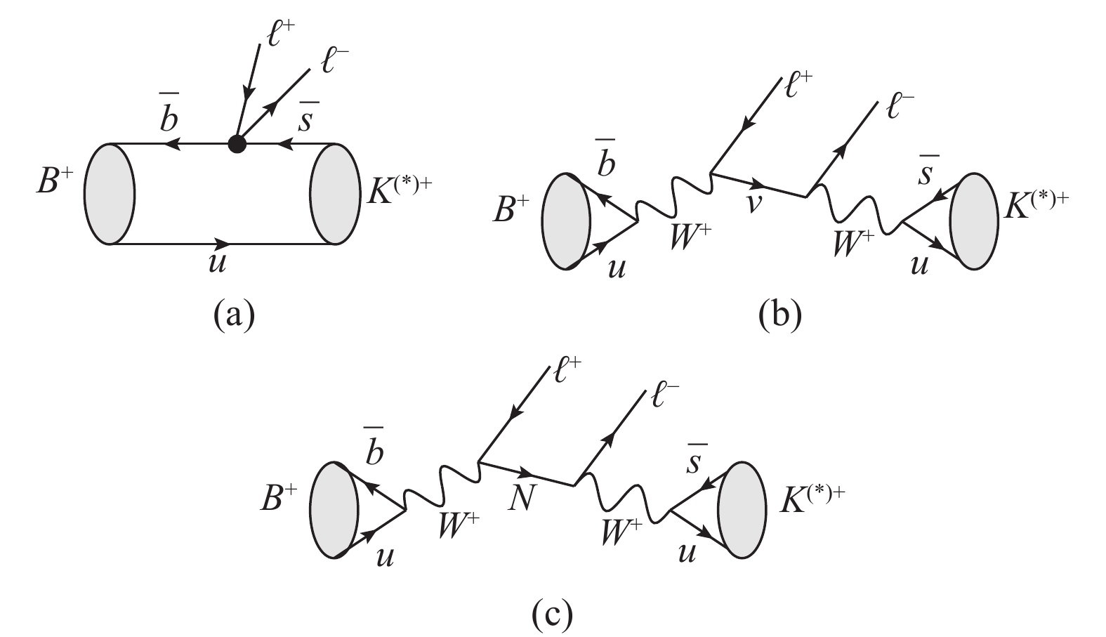
Figure 1. Feynman diagrams for the opposite-sign dilepton B meson rare decays
${B^{+}\to K^{(*)+}\ell^{+}\ell^{-}}$ . The solid circle stands for the effective vertex of the leading-order${b\to s\ell^+\ell^-}$ transition and N denotes the Majorana neutrino.$ \begin{split} { M}\left(\bar b \to \bar s{\ell ^ + }{\ell ^ - }\right) =& \displaystyle\frac{{{G_F}\alpha }}{{\sqrt 2 \pi }}V_{tb}^*{V_{ts}}\Bigg\{ C_9^{\rm eff}\left[\bar b{\gamma _\mu }{P_L}s\right]\left[\bar \ell {\gamma ^{\,\mu} }\ell\right]\\ & + {C_{10}}\left[\bar b{\gamma _\mu }{P_L}s\right]\left[\bar \ell {\gamma ^{\,\mu} }{\gamma _5}\ell\right]\\ & - \left. {2C_7^{\rm eff}{m_b}\left[{\bar bi{\sigma _{\mu \nu }}\displaystyle\frac{{{q^\nu }}}{s}{P_R}s} \right]\left[\bar \ell {\gamma ^{\,\mu} }\ell\right]} \right\}. \end{split} $

(2) Here,
$P_L=(1-\gamma_{5})/2$ ,$P_R=(1+\gamma_{5})/2$ ,$s=q^{2}=(p_1+p_2)^2$ . We take$m_s/m_b=0$ .$G_{F}$ is the Fermi coupling constant,$\alpha$ is the fine-structure constant, and$V_{q_{1}q_{2}}$ is the CKM matrix element. All Wilson coefficients$C_{i}$ , except$C_{9}^{\rm eff}$ , have the same analytic expressions as those used in the$b\to s$ transition processes [56], while$C_{9}^{\rm eff}$ can be found in [57] for the next-to-leading order approximation. The values of the Wilson coefficients used in this work are listed in Table 1. Generally, exclusive decays$B\to K^{(*)}\ell^{+}\ell^{-}$ are described by matrix elements of the quark operators over meson states, and the matrix elements are subsequently parametrized in terms of$B\to K^{(*)}$ form factors [45]. For the pseudoscalar$K$ meson,$B\to K$ form factors are defined as follows,C1 C2 C3 C4 C5 C6 ${C_{7}^{\rm eff}}$ 

C9 C10 −0.246 1.106 0.011 −0.025 0.007 −0.031 −0.312 4.211 −4.501 Table 1. The values of Wilson coefficients
${C_{i}(\mu)}$ in the SM with the scale${\mu=m_{b}}$ at the leading logarithmic approximation, with mW =80.4 GeV, mt=173.5 GeV, mb=4.8 GeV [22].$ \begin{split} &\langle K({p_K})|\bar s{\gamma _\mu }b|B({p_B})\rangle = {({p_B} + {p_K})_\mu }f_ + ^{B \to K}({q^2})\\ &\quad + \displaystyle\frac{{m_B^2 - m_K^2}}{{{q^2}}}{q_\mu }\left(f_0^{B \to K}({q^2}) - f_ + ^{B \to K}({q^2})\right), \end{split} $

(3) $ \begin{split} &\langle K({p_K})|\bar s{\sigma _{\mu \nu }}{q^\nu }b|B({p_B})\rangle = i[{({p_B} + {p_K})_\mu }{q^2}\\ &\quad -(m_B^2-m_K^2){q_\mu }]\displaystyle\frac{{f_T^{B \to K}({q^2})}}{{{m_B} + {m_K}}}. \end{split} $

(4) Here,
$f_{+}^{B \to K}(q^2)$ ,$f_{0}^{B \to K}(q^2)$ and$f_{T}^{B \to K}(q^2)$ are vector, scalar and tensor form factors of$B\to K$ transition, respectively. For the vector meson$K^{*}$ with four-momenta$p_{K^*}$ and polarization vector$\epsilon_{\mu}$ , the semileptonic form factors of the$V-A$ current and the penguin form factors can be defined as$ \begin{split} &{K^*}({p_{{K^*}}})|\bar s{\gamma _\mu }(1 - {\gamma _5})b|B({p_B})\rangle = \quad\quad\quad\quad\quad\quad\quad\quad\\ &\quad - i\epsilon _\mu ^*({m_B} + {m_{{K^*}}}){A_1}\left({q^2}\right)\\ &\quad + i{({p_B} + {p_{{K^*}}})_\mu }({\epsilon ^*} \cdot {p_B})\displaystyle\frac{{{A_2}\left({q^2}\right)}}{{{m_B} + {m_{{K^*}}}}}\\ &\quad + i{q_\mu }({\epsilon ^*} \cdot {p_B})\frac{{2{m_{{K^*}}}}}{{{q^2}}}\left( {{A_3}\left({q^2}\right) - {A_0}\left({q^2}\right)} \right)\\ &\quad + {\varepsilon _{\mu \nu \rho \sigma }}{\epsilon ^{*\nu }}p_B^\rho p_{{K^*}}^\sigma \displaystyle\frac{{2V\left({q^2}\right)}}{{{m_B} + {m_{{K^*}}}}}, \end{split} $

(5) $ \begin{split} &\langle {K^*}({p_{{K^*}}})|\bar s{\sigma _{\mu \nu }}{q^\nu }(1 + {\gamma _5})b|B({p_B})\rangle = \\ &\quad i{\varepsilon _{\mu \nu \rho \sigma }}{\epsilon ^{*\nu }}p_B^\rho p_{{K^*}}^\sigma 2{T_1}\left({q^2}\right)\\ &\quad + {T_2}\left({q^2}\right)\left\{ {\epsilon _\mu ^*\left(m_B^2 - m_{{K^*}}^2\right) - ({\epsilon ^*} \cdot {p_B}){{({p_B} + {p_{{K^*}}})}_\mu }} \right\}\\ &\quad + {T_3}\left({q^2}\right)({\epsilon ^*} \cdot {p_B})\left\{ {{q_\mu } - \displaystyle\frac{{{q^2}}}{{m_B^2 - m_{{K^*}}^2}}{{({p_B} + {p_{{K^*}}})}_\mu }} \right\}, \end{split} $

(6) with
$ \begin{split} &\langle {K^*}|{\partial _\mu }{A^\mu }|B\rangle = 2{m_{{K^*}}}({\epsilon ^*} \cdot {p_B}){A_0}\left({q^2}\right), \\ &{A_3}\left({q^2}\right) = \displaystyle\frac{{{m_B} + {m_{{K^*}}}}}{{2{m_{{K^*}}}}}{A_1}\left({q^2}\right) - \displaystyle\frac{{{m_B} - {m_{{K^*}}}}}{{2{m_{{K^*}}}}}{A_2}\left({q^2}\right), \\ &{A_0}(0) = {A_3}(0), \;\;\;\;\;\;\;{T_1}(0) = {T_2}(0). \end{split} $

(7) Using the above definition of the form factors, the decay amplitudes for
$B^{+} \to K^{(*)+}\ell^{+}\ell^{-}$ corresponding to Fig. 1(a) can be obtained,$ \begin{split} &{{ M}_a}({B^ + } \to {K^{(*) + }}{\ell ^ + }{\ell ^ - }) = \displaystyle\frac{{{G_F}\alpha }}{{\sqrt 2 \pi }}V_{ts}^*{V_{tb}} [\bar u({p_2}){\gamma _\mu }({A_{{K^{(*)}}}}\\ &\quad + {B_{{K^{(*)}}}}{\gamma _5})v({p_1}) + {m_\ell }\bar u({p_2}){D_{{K^{(*)}}}}{\gamma _5}v({p_1})], \end{split} $

(8) with
$ \begin{split} &\begin{split}{A_K} =& {p_B}\Bigg[{C_9^{\rm eff}f_ + ^{B \to K}\left({q^2}\right)} \\ &\left. { + 2C_7^{\rm eff}\displaystyle\frac{{{m_b}}}{{{m_B} + {m_K}}}f_T^{B \to K}\left({q^2}\right)} \right], \end{split}\\ &{B_K} = {p_B}{C_{10}}f_ + ^{B \to K}\left({q^2}\right), \\ &\begin{split}{D_K} =& {C_{10}}\frac{{m_B^2 - m_K^2}}{{{q^2}}}\left( {f_0^{B \to K}\left({q^2}\right) - f_ + ^{B \to K}\left({q^2}\right)} \right)\\ & - {C_{10}}f_ + ^{B \to K}\left({q^2}\right)\end{split} \end{split} $

(9) for the pseudoscalar meson
$K$ , and$ \begin{split} &\begin{split}{A_{{K^*}}} =& [A{\varepsilon _{\mu \nu \rho \sigma }}{\epsilon^{*\nu }}p_B^\rho p_{{K^*}}^\sigma-iBAA_\mu ^* + iC({\epsilon^*} \cdot {p_B})({p_B}\\ & + {p_{{K^*}}}{)_\mu } + iD({\epsilon^*} \cdot {p_B}){({p_B}-{p_{{K^*}}})_\mu }]/2, \end{split}\\ &\begin{split}{B_{{K^*}}} =& [E{\varepsilon _{\mu \nu \rho \sigma }}{\epsilon^{*\nu }}p_B^\rho p_{{K^*}}^\sigma-iFAA_\mu ^* + iG({\epsilon^*} \cdot {p_B})({p_B}\\ & + {p_{{K^*}}}{)_\mu } + iH({\epsilon^*} \cdot {p_B}){({p_B}-{p_{{K^*}}})_\mu }]/2, \end{split}\\ &{D_{{K^*}}} = 0 \end{split} $

(10) for the vector meson
$K^{*}$ . Here,$ \begin{split} &A = \displaystyle\frac{2}{{{m_B} + {m_{{K^*}}}}}C_9^{\rm eff}V\left({q^2}\right) + \displaystyle\frac{{4{m_b}}}{{{q^2}}}C_7^{\rm eff}{T_1}\left({q^2}\right), \\ &\begin{split}B =& ({m_B} + {m_{{K^*}}})\left[{C_9^{\rm eff}{A_1}\left({q^2}\right)} \right.\\ &\left. { + \frac{{2{m_b}}}{{{q^2}}}({m_B}-{m_{{K^*}}})C_7^{\rm eff}{T_2}\left({q^2}\right)} \right], \end{split}\\ &\begin{split}C = &\displaystyle\frac{1}{{m_B^2 - m_{{K^*}}^2}}\left[{({m_B}-{m_{{K^*}}})C_9^{\rm eff}{A_2}\left({q^2}\right)} \right.\\ &\left. {+ 2{m_b}C_7^{\rm eff}\left( {{T_3}({q^2}) + \frac{{m_B^2-m_{{K^*}}^2}}{{{q^2}}}{T_2}\left({q^2}\right)} \right)} \right], \end{split}\\ &\begin{split}D =& \displaystyle\frac{1}{{{q^2}}}\left[{C_9^{\rm eff}\left( {({m_B} + {m_{{K^*}}}){A_1}\left({q^2}\right)} \right.} \right.\\ &\left. {-({m_B}-{m_{{K^*}}}){A_2}\left({q^2}\right)-2{m_{{K^*}}}{A_0}\left({q^2}\right)} \right)\\ &\left. { - 2{m_b}C_7^{\rm eff}{T_3}\left({q^2}\right)} \right], \end{split}\\ &E = \displaystyle\frac{2}{{{m_B} + {m_{{K^*}}}}}{C_{10}}V\left({q^2}\right), \\ &F = ({m_B} + {m_{{K^*}}}){C_{10}}{A_1}\left({q^2}\right), \\ &G = \displaystyle\frac{1}{{{m_B} + {m_{{K^*}}}}}{C_{10}}{A_2}\left({q^2}\right), \\\end{split} $

$ \begin{split} &\begin{split}H =& \displaystyle\frac{1}{{{q^2}}}{C_{10}}\left[{({m_B} + {m_{{K^*}}}){A_1}\left({q^2}\right)} \right.\qquad\qquad\qquad\qquad\\ &\left. {-({m_B}-{m_{{K^*}}}){A_2}\left({q^2}\right)-2{m_{{K^*}}}{A_0}\left({q^2}\right)} \right].\end{split} \end{split} $

(11) The contributions from the light and heavy neutrinos are shown by the Feynman diagrams in Fig. 1(b) and Fig. 1(c), respectively. For simplification, we assume that only one heavy Majorana neutrino
$N$ exists in Type-I seesaw model, with a mass$m_{K^{(*)}} < m_N < m_B$ . The decay amplitudes for$B^{+}\to K^{(*)+}\ell^{+}\ell^{-}$ corresponding to Fig. 1(b) and Fig. 1(c) can be expressed as$ \begin{split} &{{ M}_b}({B^ + } \to {K^{(*) + }}{\ell ^ + }{\ell ^ - }) = - G_F^2V_{us}^*{V_{ub}}{f_B}{f_{{K^{(*)}}}} \\ &\quad \times\displaystyle\frac{{\bar u({p_2}){Q^{{K^{(*)}}}}p{/_\nu }p{/_B}(1 - {\gamma _5})v({p_1})}}{{p_\nu ^2}}, \end{split} $

(12) $ \begin{split} &{{ M}_c}({B^ + } \to {K^{(*) + }}{\ell ^ + }{\ell ^ - }) = iG_F^2V_{us}^*{V_{ub}}V_{\ell N}^2{f_B}{f_{{K^{(*)}}}} \\ &\quad \times\frac{{\bar u({p_2}){Q^{{K^{(*)}}}}p{/_N}p{/_B}(1 - {\gamma _5})v({p_1})}}{{p_N^2 - m_N^2 + i{\Gamma _N}{m_N}}}, \end{split} $

(13) where
$Q^{K}=p/_{K}$ and$Q^{K^{*}}=-im_{K^{*}}\varepsilon/^{*}$ .$ f_{B}~(f_{K}, ~f_{K^*}) $ is the decay constant of$B~(K, ~K^*)$ meson.$p_{\nu}$ and$p_{N}$ stand for the four-momenta of the light$\nu$ and heavy neutrino$N$ , respectively.$\Gamma_{N} \approx 2 \sum_{\ell} |V_{\ell N}|^2 (m_N/m_{\tau})^5 \times \Gamma_{\tau}$ represents the total decay width of a Majorana neutrino with$V_{\ell N}$ denoting the mixing matrix element between$\ell$ and$N$ [19]. The decay rates can be written as$ \begin{split} &{\cal B}({B^ + } \to {K^{(*) + }}{\ell ^ + }{\ell ^ - }) \\ = & \displaystyle\frac{{{\tau _B}}}{{2{m_B}{{(2\pi )}^5}}}\int | {\cal M}{|^2} \displaystyle\frac{{|\vec p_1^B|}}{{4{m_B}}}\displaystyle\frac{{|\vec p_2^*|}}{{4\sqrt {{s_{2{K^{(*)}}}}} }}{\rm d}\Omega _1^B{\rm d}\Omega _2^*{\rm d}{s_{2{K^{(*)}}}}, \end{split} $

(14) with the total decay amplitude
$\cal{M} = \cal{M}_{a} + \cal{M}_{b} + \cal{M}_{c}$ , where$\vec{p}_{1}^{\, B}$ ($\vec{p}_{2}^{\, \, *}$ ) and${\rm d}\Omega_{1}^{B}$ (${\rm d}\Omega_{2}^{*}$ ) denote the 3-momentum and solid angle of charged lepton$\ell^{+}$ ($\ell^{-}$ ) in the rest frame of the B meson ($\ell^{-}K^{(*)}$ system), respectively.We find that the contributions from Fig. 1(b)and from the interference terms are about five orders smaller than from the SM, and can be neglected.The same-sign
$\Delta L=2~$ LNV processes$B^{+}(p_B)\to$ $ K^{(*)-} (p_{K^{(*)}}) \ell^{+}(p_{1}) \ell^{+}(p_{2}) $ are more sensitive to new physics models. These decay channels may occur via Majorana neutrino exchange, and provide an especially clear signal if the mediator Majorana neutrino is on-shell. The dominant contribution is from the Feynman diagram inFig. 2(a), while the contribution from Fig. 2(b)is small enough to be neglected, as concluded in [21, 22]. The corresponding decay amplitudes of$B^{+}\to K^{(*)-}\ell^{+}\ell^{+}$ are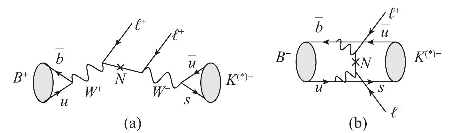
Figure 2. Feynman diagrams for
${B^{+}\to K^{(*)-}\ell^{+}\ell^{+}}$ via Majorana neutrino exchange.$ \begin{split} &{ M}({B^ + } \to {K^{(*) - }}{\ell ^ + }{\ell ^ + }) = - iG_F^2V_{us}^*{V_{ub}}V_{\ell N}^2{f_B}{f_K}{m_N} \\ & \quad \times\left[{\displaystyle\frac{{\bar u({p_2}){Q^{{K^{(*)}}}}p{/_B}(1-{\gamma _5})v({p_1})}}{{p_N^2-m_N^2 + i{\Gamma _N}{m_N}}}} \right.\\ & \quad \left. { +\displaystyle \frac{{\bar u({p_2})p{/_B}{Q^{{K^{(*)}}}}(1-{\gamma _5})v({p_1})}}{{p_N^{\prime 2} - m_N^2 + i{\Gamma _N}{m_N}}}} \right]. \end{split} $

(15) The branching ratios of the same-sign charged dilepton decays can be readily obtained in the same way as in Eq. (14), except that a factor 1/2 should be included since there are two identical particles in the final state.
-
The
$B\to K$ form factors are parameterized by the following formulae [58],$ f_{+(T)}^{B\to K}\left(q^2\right)=\frac{r_1}{1-q^2/m_{\rm{fit}}^2} +\frac{r_2}{1-q^2/m_{B_s^*(1^-)}^2}, $

(16) $ f_{0}^{B\to K}\left(q^2\right)=\frac{r_2}{1-q^2/m_{\rm{fit}}^2}\, , $

(17) where
$m_{B_s^*(1^-)}=5.413 $ GeV is the mass of the$B_s^*(1^-)$ . The values of other parameters$r_{1(2)}$ and$m_{\rm{fit}}^2$ are given in Table 2. The parameters for$B\to K^*$ form factors are obtained from the calculation of AdS/QCD at low-to-intermediate$q^2$ , and from the lattice data at high$q^2$ [49]. The seven independent form factors can be expressed as${f_{+}^{B\to K}}$ 

${f_{T}^{B\to K}}$ 

${f_{0}^{B\to K}}$ 

${r_{1}}$ 

0.8182 0.893 − ${r_{2}}$ 

−0.4862 −0.5073 0.332 ${m_{\rm{fit}}^2}$ 

41.61 33.13 61.64 Table 2. The inputs of
${r_1}$ ,${r_2}$ and${m_{\rm fit}^2}$ for${B\to K}$ form factors [58].$ F\left(q^2\right)=\frac{F(0)}{1-a\, q^2/m_B^2+b\, q^4/m_B^4}, $

(18) where
$F$ stands for$A_0$ ,$A_1$ ,$A_2$ ,$T_1$ ,$T_2$ ,$T_3$ ,$V$ . The corresponding values of$F(0)$ ,$a$ ,$b$ are listed in Table 3.A0 A1 A2 T1 T2 T3 V F(0) 0.243 0.244 0.244 0.258 0.239 0.157 0.297 a 1.618 0.586 1.910 1.910 0.525 1.147 1.934 b 0.561 −0.356 1.498 1.082 −0.459 −0.114 1.089 Table 3. The inputs of F(0) (form factor at q2=0), a and b for
$\scriptstyle{B\to K^*}$ form factors A0, A1, A2, T1, T2,T3 and V [49].In our numerical calculations, we only focus on dimuon decay channels, having in mind the relatively high muon reconstruction ability of the LHCb experiment. The CKM matrix elements are obtained by the Wolfenstein parametrization. The values of the Wolfenstein parameters (
$\lambda$ ,$A^{\prime}$ ,$\bar{\rho}$ ,$\bar{\eta}$ ) , and of the other parameters used, are listed in Table 4. We assume an optimistic case with$|V_{\mu N}|^2\gg |V_{\tau N}|^2, ~|V_{e N}|^2$ , so that the interactions are completely determined by the mixing matrix element$|V_{\mu N}|^2$ [18].${G_{F}}$ 

1.16637×10⁻⁵ GeV−2 ${\alpha}$ 

1/137 ${\tau_{B}}$ 

1.638 ps ${m_{c}}$ 

1.27 GeV ${\Gamma_{\tau}}$ 

2.267×10⁻¹² GeV ${m_{\tau}}$ 

1.777 GeV ${f_{K}}$ 

155.6 MeV ${m_{K}}$ 

0.4937 GeV ${f_{K^*}}$ 

225 MeV [60] ${m_{K^*}}$ 

0.892 GeV ${f_{B}}$ 

187.1 MeV ${m_{B}}$ 

5.28 GeV ${\lambda}$ 

0.225±0.0006 ${A^{\prime}}$ 

0.811±0.015 ${\bar{\rho}}$ 

0.124±0.024 ${\bar{\eta}}$ 

0.356±0.015 Table 4. Input parameters used in our numerical calculation [59].
The SM dilepton invariant mass distributions
${\rm d} {B}( B^{+}\to K^{(*)+}\mu^+\mu^-)/{{\rm d}{q^2}}$ are shown in Fig. 3(a). The distributions for${\rm d}{ {B}}({ B}^{+}\to { K}^{+}\mu^+\mu^-)/{\rm d}{q^2}$ and${\rm d}{ {B}}({ B}^{+}\to $ ${ K}^{*+}\mu^+\mu^-)/{\rm d}{q^2} $ are distinct because the form factors and the amplitudes are different for scalar and vector mesons. The integrated branching ratios are$ \begin{split} &{{ B}_{\rm SM}}({B^ + } \to {K^ + }{\mu ^ + }{\mu ^ - }) = (5.21 \pm 0.51) \times {10^{ - 7}}, \\ &{{ B}_{\rm SM}}({B^ + } \to {K^{* + }}{\mu ^ + }{\mu ^ - }) = \left(7.63_{ - 0.68}^{ + 0.69}\right) \times {10^{ - 7}}, \end{split} $

(19) where the dominant uncertainty comes from the CKM matrix elements and the renormalization scale variation. Experimentally, the most precise measurements of the differential branching fractions of
$B^{+}\to K^{(*)+}\mu^+\mu^-$ have been performed using a data set with 3 fb-1 of integrated luminosity collected by the LHCb detector [43]. The corresponding integrated branching fractions are$ \begin{split} { B}({B^ + } \to {K^ + }{\mu ^ + }{\mu ^ - }) = \qquad\qquad\qquad\qquad\\ \quad (4.29 \pm 0.07({\rm{stat}}) \pm 0.21({\rm{syst}})) \times {10^{ - 7}}, \end{split} $

$ \begin{split} { B}({B^ + } \to {K^{* + }}{\mu ^ + }{\mu ^ - }) = \qquad\qquad\qquad\qquad\\ \quad (9.24 \pm 0.93({\rm{stat}}) \pm 0.67({\rm{syst}})) \times {10^{ - 7}}. \end{split} $

(20) Our SM predictions for
$B^{+}\to K^{(*)+}\mu^+\mu^-$ are therefore roughly consistent with the most recent LHCb data, within the range of experimental and theoretical errors, and comparable to the other SM calculation results [44, 45, 48, 55]. The angular distributions of the opposite-sign leptons are plotted in Fig. 3(b) in the$B$ meson rest frame. If enough events are collected, this kind of distribution is a significant element for studying the interactions.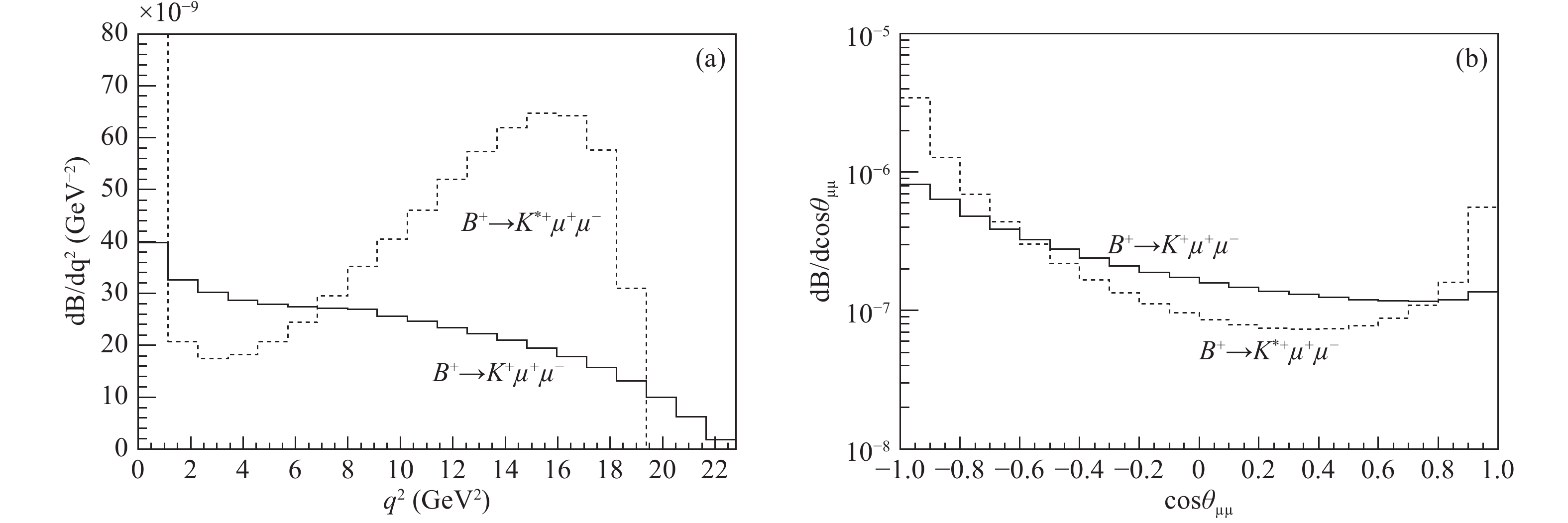
Figure 3. (a) The invariant mass distributions and (b) the angular distributions of the opposite-sign dilepton for
${{B}(B^{+}\to K^{(*)+}\mu^{+}\mu^{-})}$ in the SM.Given the Majorana neutrino contributions, the only difference between the same-sign decay and the opposite-sign decay is that a diagram with lepton exchange should be taken into account if they are identical particles. However, this discrepancy disappears after integrating over the phase space. Therefore, the contributions from Fig. 1(c) to
$B^{+}\to K^{(*)+}\mu^{+}\mu^{-}$ are the same as the contributions from Fig. 2(a) to$B^{+}\to K^{(*)-}\mu^{+}\mu^{+}$ . For this reason, we discuss the numerical results of Fig. 1(c) together with the LNV processes$B^{+}\to K^{(*)-}\mu^{+}\mu^{+}$ below.The branching ratios for LNV processes depend on two new parameters, the mixing matrix element
$V_{\mu N}$ and Majorana neutrino mass$m_N$ . The simplified branching ratios$\bar{{B}}(B^{+}\to K^{(*)-} \mu^{+} \mu^{+}) = {{B}} ({ B}^{+} \to { K}^{(*)-} \mu^{+} \mu^{+}) / |{\cal V}_{\mu N}|^2$ are plotted as function of Majorana neutrino mass$m_N$ in Fig. 4. The peaks are around 2 GeV, depending on the kinematical distributions related to the masses of$B$ and$K^{(*)}$ mesons. Once the Majorana neutrino mass and the mixing matrix element are fixed, the branching ratios of$B^{+}\to K^{(*)-}\mu^{+}\mu^{+}$ can be obtained. With the precise measurement of$B$ meson decays, the LHCb and BaBar collaborations have reported the upper limits for the LNV rare decays$B^{+}\to K^{(*)-}\mu^{+}\mu^{+}$ [61, 62],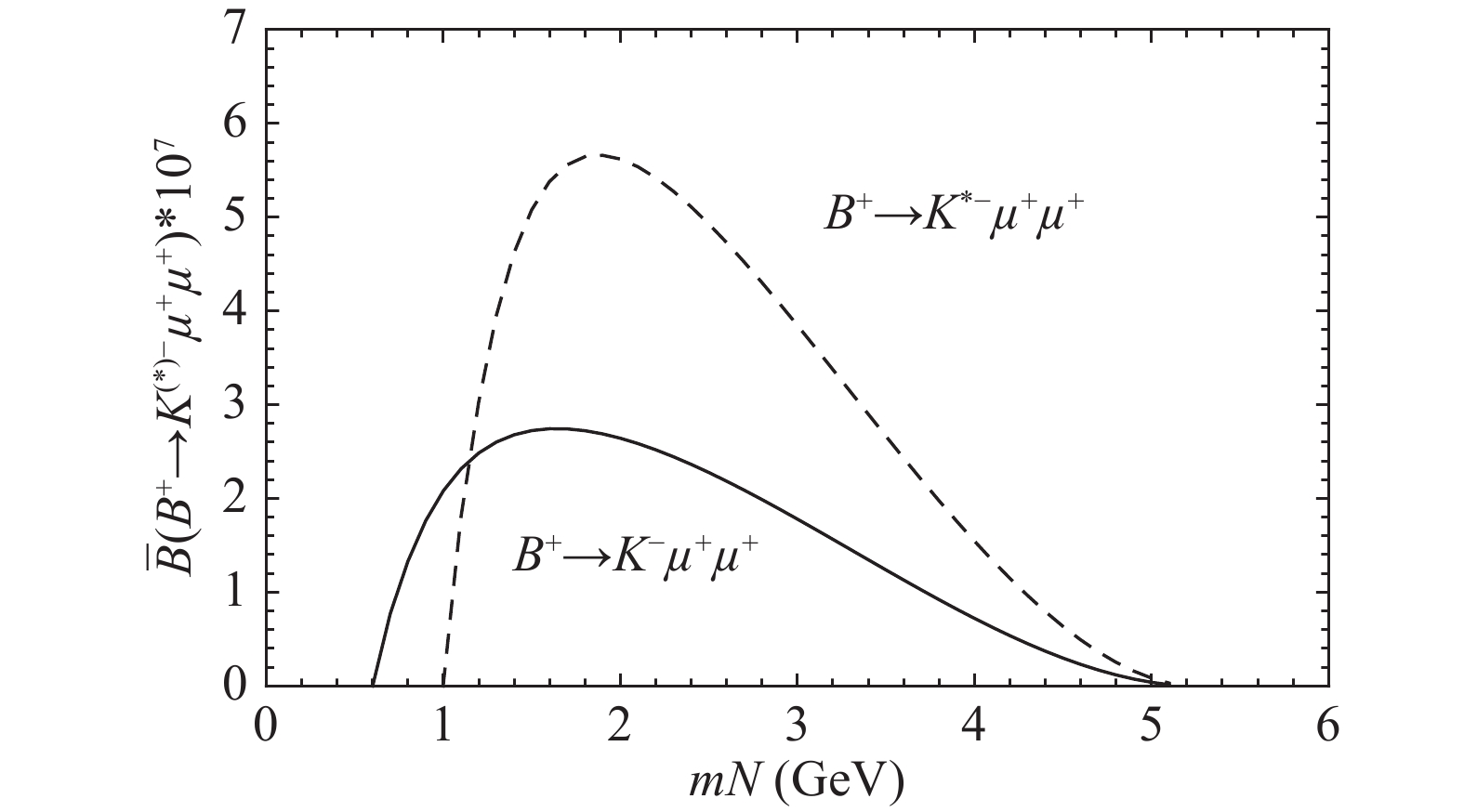
Figure 4. Simplified branching ratios
${\bar{{B}}(B^{+}\to K^{(*)-} \mu^{+} \mu^{+}) = }$ ${{B} (B^{+} \to K^{(*)-} \mu^{+} \mu^{+}) / |V_{\mu N}|^2}$ with respect to Majorana neutrino mass m N.$ { B}({B^ + } \to {K^ - }{\mkern 1mu} {\mu ^ + }{\mkern 1mu} {\mu ^ + }) < 4.1 \times {10^{ - 8}}\;\;\;\;{\rm{at}}\;{\rm{90}}{\text \%} \;{\rm{C}}.{\rm{L}}., $

(21) $ { B}({B^ + } \to {K^{* - }}{\mu ^ + }{\mu ^ + }) < 5.9 \times {10^{ - 7}}\;\;\;{\rm{at}}\;{\rm{90}}{\text\%} \;{\rm{C}}.{\rm{L}}., $

(22) which can be used to constrain the parameter space for the mixing matrix element
$V_{\mu N}$ and Majorana neutrino mass$m_N$ . Given that the LHCb collaboration has determined the branching ratio${B}(B^{-}\to \pi^{+}\mu^{-}\mu^{-})\leqslant$ 4.0 × 10⁻⁹ at 95% C.L. [10], we plot the excluded parameter regions in the$|V_{\mu N}|^2$ versus$m_N$ plane in Fig. 5. The region above the dashed (solid) line is excluded by LHCb with LNV process$B^{+} \to K^{-}(\pi^{-}) \mu^{+} \mu^{+}$ at 90% (95%) C.L. As shown in the figure, the LNV rare decay channel$B^{+}\to \pi^{-} \mu^{+}\mu^{+}$ provides a more rigorous constraint than the LNV$B\to K$ channel because the$B^{+}\to \pi^{-} \mu^{+}\mu^{+}$ process is much less suppressed by the CKM factors than$B^{+}\to K^{(*)-}\mu^{+}\mu^{+}$ . However, the bounds for the new physics parameters are less strict with the presently available data for$B^{+}\to K^{*-}\mu^+\mu^+$ process.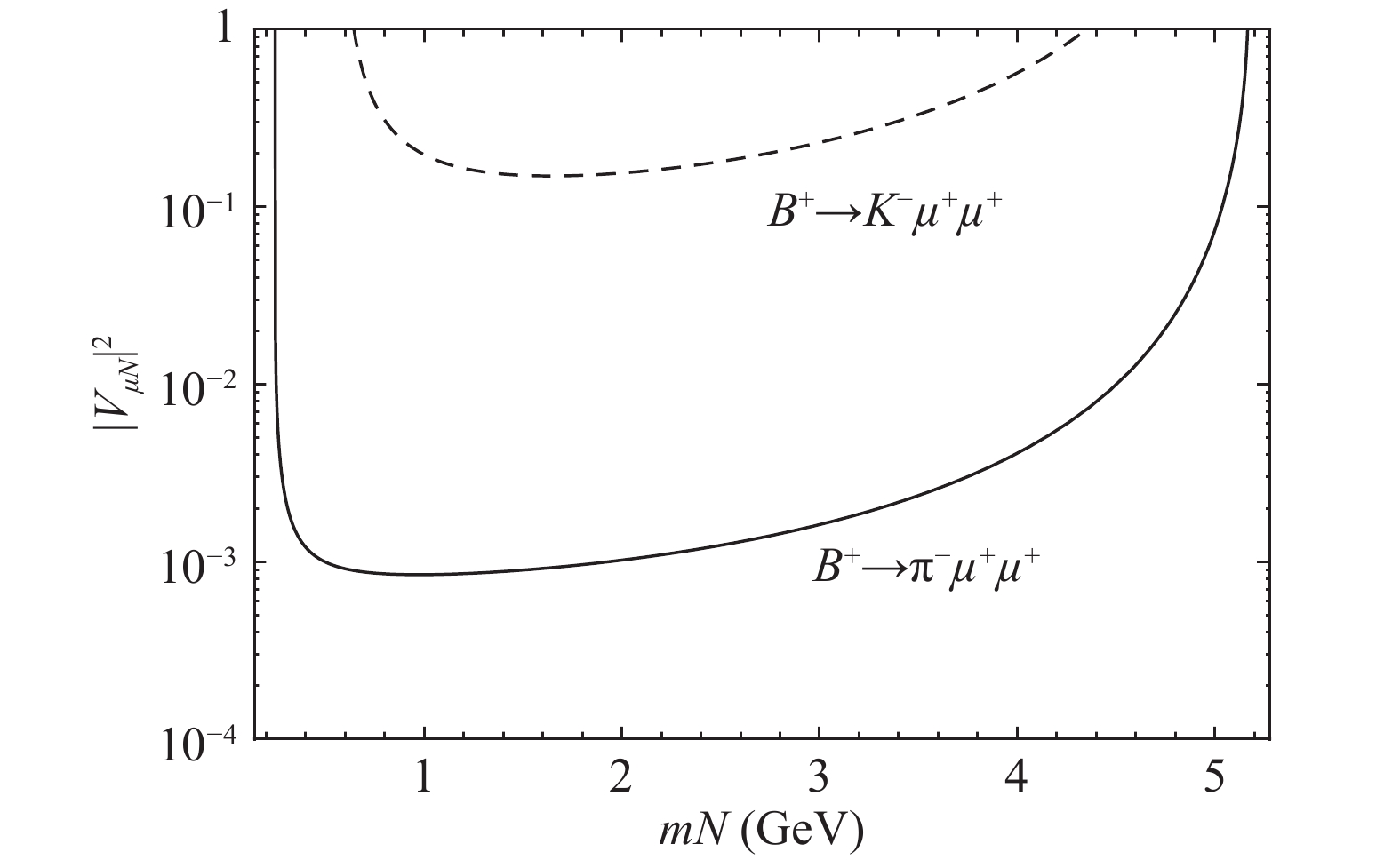
Figure 5. Contour plot obtained from the experimental upper limits for LNV rare decays
${B^{+}\to K^{-}\mu^{+}\mu^{+}}$ and${B^{+}\to \pi^{-}\mu^{+}\mu^{+}}$ .The best fit values of
$|V_{\mu N}|^{2}$ and$m_{N}$ , obtained in our previous work [22] for$ B^+\to \pi^-\mu^+\mu^+ $ , agree with the LHCb upper limit [10]. As a result, we list in Table 5 the branching ratios for LNV processes$B^{+}\to K^{(*)-}\mu^{+}\mu^{+}$ with the best fit values of$|V_{\mu N}|^{2}$ and$m_{N}$ . Three cases are shown, corresponding to the form factors obtained with heavy quark symmetry and lattice QCD method (HQS+LQCD), perturbative QCD method (PQCD), and light cone QCD sum rule method (LCSR) [22]. We choose three typical values of$m_N$ in each case to estimate the branching ratios. The Table shows that the branching ratios of LNV processes$B^{+}\to K^{(*)-}\mu^{+}\mu^{+}$ induced by Majorana neutrino exchange are in agreement with the LHCb (BaBar) measurements. Furthermore, the values are such that they are possibly accessible at the future B-factory experiment with high integrated luminosity. The branching ratios of opposite-sign$B^{+}\to K^{(*)+}\mu^{+}\mu^{-}$ processes induced by a Majorana neutrino (contributions from Fig. 1(c)) are the same as the same-sign processes$B^{+}\to K^{(*)-}\mu^{+}\mu^{+}$ , which are a few orders smaller than the SM contributions. The numerical results from the interference terms are several orders smaller than from Fig. 1(c), and we can safely neglect them. Once the LNV processes are observed, the differential distributions should be studied. In Fig. 6, the invariant mass distributions and angular distributions of the same-sign dilepton process$\bar{{B}}(B^{+}\to K^{(*)-} \mu^{+} \mu^{+})$ with$m_N$ =2 GeV are presented. The same-sign process has a different distribution compared to the opposite-sign process. These distributions could be used to investigate the decay properties of hadrons, and provide hints for new physics models.
Figure 6. (a) The invariant mass distributions and (b) the angular distributions of the same-sign dilepton for
${\bar{\cal{B}}(B^{+}\to K^{(*)-} \mu^{+} \mu^{+})}$ with mN=2 GeV.${m_N}$ 

${|V_{\mu N}|^{2}}$ 

${B^{+}\to K^{-}\mu^{+}\mu^{+}}$ 

${B^{+}\to K^{*-}\mu^{+}\mu^{+}}$ 

HQS+LQCD 1 GeV 8.52×10⁻⁴ 1.78×10⁻¹⁰ 1.50×10⁻¹¹ 2 GeV 1.03×10⁻³ 2.73×10⁻¹⁰ 5.79×10⁻¹⁰ 3 GeV 1.63×10⁻³ 2.90×10⁻¹⁰ 6.27×10⁻¹⁰
PQCD 1 GeV 7.10×10⁻⁴ 1.48×10⁻¹⁰ 1.25×10⁻¹¹ 2 GeV 8.58×10⁻⁴ 2.27×10⁻¹⁰ 4.82×10⁻¹⁰ 3 GeV 1.36×10⁻³ 2.42×10⁻¹⁰ 5.23×10⁻¹⁰
LCSR 1 GeV 1.33×10⁻⁴ 2.77×10⁻¹¹ 2.35×10⁻¹² 2 GeV 1.61×10⁻⁴ 4.26×10⁻¹¹ 9.05×10⁻¹¹ 3 GeV 2.55×10⁻⁴ 4.54×10⁻¹¹ 9.81×10⁻¹¹ Table 5. Majorana neutrino contributions to the branching ratios of
${B^{+}\to K^{(*)-}\mu^{+}\mu^{+}}$ . The${m_N}$ and${|V_{\mu N}|^{2}}$ are the best fits corresponding to heavy quark symmetry and lattice QCD method (HQS+LQCD), perturbative QCD method (PQCD) and light cone QCD sum rule method (LCSR), see [ 22]. -
LNV processes have been widely studied in the search for new physics beyond the SM. The intermediate Majorana neutrino exchange LNV processes provide evidence for the Majorana nature of neutrinos. With the precision measurements of the B meson decays, the
$\Delta L=2$ semileptonic decay processes have been extensively calculated for hints of new physics. We studied the$B^{+} \to K^{(*)+}\mu^+\mu^-$ process, both in the SM and Type-I seesaw model. The decay branching ratios are roughly consistent with the experimental measurements. We also investigated the LNV decays$B^{+}\to K^{(*)-}\mu^{+}\mu^+$ . Parameter constraints on$m_N$ and$|V_{\mu N}|^2$ , obtained from the experimental upper limits for$B^{+}\to K^{(*)-}\mu^+\mu^+$ processes, are less strict than the constraints from the$B\to \pi$ process. Thus, using the best fits for Majorana neutrino mass$m_{N}$ and mixing matrix elements$|V_{\mu N}|^{2}$ obtained in our previous work, we found the branching ratio of the same-sign charged dilepton process$B^{+}\to K^{(*)-}\mu^{+}\mu^+$ , which is lower than the LHCb (BaBar) upper limits obtained in 2012 (2014). The Majorana neutrino contributions to the branching ratios of$B^{+}\to K^{(*)+}\mu^+\mu^-$ are found to be small compared to the SM contributions. Once the LNV processes are observed in future experiment with high luminosity, the dilepton invariant mass distributions as well as the dilepton angular distributions could shed light on the properties of new physics interactions.
Study of the Standard Model and Majorana neutrino contributions to ${ B}^{{ +}} { \to} { K}^{{ (*){ \pm}}}{ \mu}^{ +}{ \mu}^{{ \mp}}$
- Received Date: 2018-09-30
- Available Online: 2019-02-01
Abstract: Lepton number violation processes can be induced by the Majorana neutrino exchange, which provide evidence for the Majorana nature of neutrinos. In addition to the natural explanation of the small neutrino masses, Type-I seesaw mechanism predicts the existence of Majorana neutrinos. The aim of this work is to study the B meson rare decays


 DownLoad: