


 Abstract
 HTML
HTML Reference
 Related
 PDF
PDF


-
Many exotic hadrons have been discovered in the past decade owing to significant experimental progresses [1], such as the two hidden-charm pentaquark resonances
$ P_c(4380) $ and$ P_c(4450) $ discovered by the LHCb Collaboration [2-5]. More exotic hadrons are likely to be observed in the future by BaBar, Belle, BESIII, CMS, and LHCb experiments, etc. They are new blocks of QCD matter, providing insights to deepen our understanding of the non-perturbative QCD, and their relevant theoretical and experimental studies have opened a new page for hadron physics [6-11].In the past year, to investigate their nature,
$ P_c(4380) $ and$ P_c(4450) $ have been studied using various methods and models. There are many possible interpretations, such as meson-baryon molecules [12-23], compact diquark-diquark-antiquark pentaquarks [24-27], compact diquark-triquark pentaquarks [28, 29], genuine multiquark states other than molecules [30-35], and kinematical effects related to thresholds and triangle singularity [36-40]. Their productions and decay properties are also interesting [41-53]. More extensive discussions can be found in Refs. [54-56].The preferred spin-parity assignments for the
$ P_c(4380) $ and$ P_c(4450) $ states were suggested to be$ (3/2^-, 5/2^+) $ ; however, some other assignments, such as$ (3/2^+, 5/2^-) $ and$ (5/2^+, 3/2^-) $ , have also been suggested by the LHCb Collaboration [2]. It is useful to theoretically study all possible assignments to better understand their properties.In this study, we use the method of QCD sum rule to study the possible spin-parity assignments of
$ P_c(4380) $ and$ P_c(4450) $ . However, first, we reinvestigate our previous studies on$ P_c(4380) $ and$ P_c(4450) $ [57, 58] by requiring the pole contribution (PC) to be greater than or equal to 30% in order to ensure that the one-pole parametrization is valid; this value was just 10% in our previous studies [57, 58]. Note that there have been some experimental data on exotic hadrons; however, they are not sufficient, and more experimental results are necessary to make our theoretical analyses more reliable.The remainder of this paper is organized as follows: the above reinvestigation is presented in Section 2, numerical analyses are presented in Section 3, the investigation of hidden-charm pentaquark states of
$ J^P = 3/2^+ $ and$ J^P = 5/2^- $ are provided in Section 4, and the results will be discussed and summarized in Section 5. -
All the local hidden-charm pentaquark interpolating currents have been systematically constructed in Refs. [57, 58]. Some of these currents were selected to perform QCD sum rule analyses. The results suggest that
$ P_c(4380) $ and$ P_c(4450) $ can be interpreted as hidden-charm pentaquark states composed of anti-charmed mesons and charmed baryons. However, the analyses therein used one criterion, which was not optimized. The condition was that the PC should be greater than 10% to ensure that the one-pole parametrization was valid. This value is not so significant, and accordingly, the question arises whether we can find a larger PC to better ensure one-pole parametrizationIn the present study, we try to answer this question to find better (more reliable) QCD sum rule results. In particular, we find the following two mixing currents:
$ \begin{split} J_{\mu, 3/2-} =& \cos\theta_1 \times \xi_{36\mu} + \sin\theta_1 \times \psi_{9\mu} \\ =& \cos\theta_1 \times [\epsilon^{abc} (u^T_a C \gamma_\nu \gamma_5 d_b) \gamma_\nu \gamma_5 c_c] [\bar c_d \gamma_\mu \gamma_5 u_d] \\ & + \sin\theta_1 \times [\epsilon^{abc} (u^T_a C \gamma_\nu u_b) \gamma_\nu \gamma_5 c_c] [\bar c_d \gamma_\mu d_d], \end{split} $

(1) $ \begin{split} J_{\mu\nu, 5/2+} =& \cos\theta_2 \times \xi_{15\mu\nu} + \sin\theta_2 \times \psi_{4\mu\nu} \\ =& \cos\theta_2 \times [\epsilon^{abc} (u^T_a C \gamma_\mu \gamma_5 d_b) c_c] [\bar c_d \gamma_\nu u_d] \\ &+ \sin\theta_2 \times [\epsilon^{abc} (u^T_a C \gamma_\mu u_b) c_c] [\bar c_d \gamma_\nu \gamma_5 d_d] + \{ \mu \leftrightarrow \nu \}, \end{split} $

(2) where
$ a \cdots d $ are color indices;$ \theta_{1/2} $ are two mixing angles;$ J_{\mu, 3/2-} $ and$ J_{\mu\nu, 5/2+} $ have the spin-parity$ J^P = 3/2^- $ and$ 5/2^+ $ , respectively. The four single currents,$ \xi_{36\mu} $ ,$ \psi_{9\mu} $ ,$ \xi_{15\mu\nu} $ , and$ \psi_{4\mu\nu} $ , were first constructed in Refs. [57, 58]. We can verify:1) The current
$ \xi_{36\mu} $ well couples to the S-wave$ [\Lambda_c(1P)\bar D_1] $ , P-wave$ [\Lambda_c(1P)\bar D] $ , P-wave$ [\Lambda_c\bar D_1] $ , D-wave$ [\Lambda_c\bar D] $ channels, etc. Here, the$ \Lambda_c(1P) $ denotes the$ \Lambda_c(2593) $ of$ J^P = 1/2^- $ and$ \Lambda_c(2625) $ of$ J^P = 3/2^- $ .2) The current
$ \psi_{9\mu} $ well couples to the S-wave$ [\Sigma_c \bar D^*] $ channel, etc.3) The current
$ \xi_{15\mu\nu} $ well couples to the S-wave$ [\Lambda_c(1P) \bar D^*] $ , P-wave$ [\Lambda_c\bar D^*] $ channels, etc.4) The current
$ \psi_{4\mu\nu} $ well couples to the S-wave$ [\Sigma_c^* \bar D_1] $ , P-wave$ [\Sigma_c^* \bar D] $ channels, etc.We use the above two mixing currents,
$ J_{\mu, 3/2-} $ and$ J_{\mu\nu, 5/2+} $ , to perform QCD sum rule analyses; the results will be given in the next section. First, we briefly introduce our approach; interested readers can refer to Refs. [59-64] for further details.First, we assume
$ J_{\mu, 3/2-} $ and$ J_{\mu\nu, 5/2+} $ couple to physical states through$ \langle 0 | J_{\mu, 3/2-} | X_{3/2-} \rangle = f_{X_{3/2-}} u_\mu (p), $

(3) $ \langle 0 | J_{\mu\nu, 5/2+} | X_{5/2+} \rangle = f_{X_{5/2+}} u_{\mu\nu} (p), $

(4) and write the two-point correlation functions as
$ \begin{split} &\Pi_{\mu \nu, 3/2-}\left(q^2\right) \\ &\;\; = i \int {\rm d}^4x {\rm e}^{{\rm i}q\cdot x} \langle 0 | T\left[J_{\mu, 3/2-}(x) \bar J_{\nu, 3/2-}(0)\right] | 0 \rangle \\ &\;\; = \left(\frac{q_\mu q_\nu}{q^2}-g_{\mu\nu}\right) (q\!\!\!\!/ + M_{X_{3/2-}}) \Pi_{3/2-}\left(q^2\right) + \cdots, \end{split} $

(5) $ \begin{split} & \Pi_{\mu \nu \rho \sigma, 5/2+}\left(q^2\right) \\&\;\; = i \int {\rm d}^4x {\rm e}^{{\rm i}q\cdot x} \langle 0 | T\left[J_{\mu\nu, 5/2+}(x) \bar J_{\rho\sigma, 5/2+}(0)\right] | 0 \rangle \\ &\;\; = \left(g_{\mu\rho}g_{\nu\sigma} + g_{\mu\sigma} g_{\nu\rho} \right) (q\!\!\!\!/ + M_{X_{5/2+}}) \Pi_{5/2+}\left(q^2\right) + \cdots, \end{split} $

(6) where
$ \cdots $ contains non-relevant spin components.Note that if the physical state has the opposite parity, the
$ \gamma_5 $ -coupling should be used [65-68]. For example, if$ \langle 0 | J_{\mu, 3/2-} | X^\prime_{3/2+} \rangle = f_{X^\prime_{3/2+}} \gamma_5 u^\prime_\mu (p), $

(7) then
$ \begin{split} &\Pi_{\mu \nu, 3/2+}\left(q^2\right) \\&\;\; = i \int {\rm d}^4x {\rm e}^{{\rm i}q\cdot x} \langle 0 | T\left[J_{\mu, 3/2-}(x) \bar J_{\nu, 3/2-}(0)\right] | 0 \rangle \\ &\;\; = \left(\frac{q_\mu q_\nu}{q^2}-g_{\mu\nu}\right) (q\!\!\!\!/ - M_{X_{3/2+}}) \Pi_{3/2+}\left(q^2\right) + \cdots . \end{split} $

(8) Hence, we can compare terms proportional to
$ {\bf{1}} \times g_{\mu\nu} $ and$ q\!\!\!\!/\times g_{\mu\nu} $ to determine the parity of$ X^{(\prime)}_{3/2\pm} $ . Accordingly, in the present study, we use terms proportional to$ {\bf{1}} \times g_{\mu\nu} $ and$ {\bf{1}} \times g_{\mu\rho} g_{\nu\sigma} $ to evaluate masses of X’s, which are then compared with those proportional to$ q\!\!\!\!/ \times g_{\mu\nu} $ and$ q\!\!\!\!/\times g_{\mu\rho} g_{\nu\sigma} $ to determine their parity.At the hadron level, we use the dispersion relation to rewrite the two-point correlation function as
$ \Pi(q^2)={\frac{1}{\pi}}\int^\infty_{s_<}\frac{{\rm Im} \Pi(s)}{s-q^2-i\varepsilon}{\rm d}s, $

(9) where
$ s_< $ is the physical threshold. Its imaginary part is defined as the spectral function, which can be evaluated by inserting the intermediate hadron states$ \sum_n|n\rangle\langle n| $ , but adopting the usual parametrization of one-pole dominance for ground state X along with a continuum contribution:$ \begin{split} \rho(s) \equiv & \frac{1}{\pi}{\rm Im}\Pi(s) = \sum_n\delta(s-M^2_n)\langle 0|J|n\rangle\langle n|{\bar J}|0\rangle \\ =& f_X^2\delta(s-m_X^2)+ {\rm{continuum}} . \end{split} $

(10) At the quark and gluon level, we substitute Eqs. (1-2) in the two-point correlation functions (5-6), and calculate them using the method of operator product expansion (OPE). In the present study, we evaluate
$ \rho(s) $ at the leading order on$ \alpha_s $ , up to eight dimensions. For this, we calculated the perturbative term, quark condensate$ \langle \bar q q \rangle $ , gluon condensate$ \langle g_s^2 GG \rangle $ , quark-gluon condensate$ \langle g_s \bar q \sigma G q \rangle $ , and their combinations$ \langle \bar q q \rangle^2 $ and$\langle \bar q q \rangle $ $ \langle g_s \bar q \sigma G q \rangle $ . We find that the D= 4 term$ m_c \langle \bar q q \rangle $ and the D= 6 term$ m_c \langle g_s \bar q \sigma G q \rangle $ are important power corrections to the correlation functions. Note that we assumed the vacuum saturation for higher dimensional operators such as$ \langle 0 | \bar q q \bar q q |0 \rangle \sim \langle 0 | \bar q q |0 \rangle \langle 0|\bar q q |0 \rangle $ , and this can lead to some systematic uncertainties.Finally, we perform the Borel transform at both the hadron and quark-gluon levels, and express the two-point correlation function as
$ \Pi^{(\rm all)}(M_B^2)\equiv\mathcal{B}_{M_B^2}\Pi(p^2) = \int^\infty_{s_<} {\rm e}^{-s/M_B^2} \rho(s) {\rm d}s . $

(11) After assuming that the continuum contribution can be well approximated by the OPE spectral density above a threshold value
$ s_0 $ , we obtain the sum rule relation$ M^2_X(s_0, M_B) = {\int^{s_0}_{s_<} {\rm e}^{-s/M_B^2} \rho(s) s {\rm d}s \over \int^{s_0}_{s_<} {\rm e}^{-s/M_B^2} \rho(s) {\rm d}s} . $

(12) We use the mixing current
$ J_{\mu, 3/2-} $ defined in Eq. (1) to perform sum rule analyses, and the terms proportional to$ {\bf{1}} \times g_{\mu\nu} $ are given in Eq. (13), where$ t_1 = \cos\theta_1 $ and$ t_2 = \sin\theta_1 $ . The terms proportional to$q\!\!\!\!/\times g_{\mu\nu} $ are listed in Eq. (14), which are almost the same as the former ones, suggesting that the state coupled by$ J_{\mu, 3/2-} $ has the spin-parity$ J^P = 3/2^- $ . Similarly, we use$ J_{\mu\nu, 5/2+} $ defined in Eq. (2) to perform sum rule analyses, and the terms proportional to$ {\bf{1}} \times g_{\mu\nu} $ and$ q\!\!\!\!/\times g_{\mu\nu} $ are listed in Eqs. (15) and (16), respectively. We find that its relevant state has the spin-parity$ J^P = 5/2^+ $ . These two sum rules will be used to perform numerical analyses in the next section.$ \begin{split} \rho_{3/2-, 1}(s) =& \rho^{\rm pert}_{3/2-, 1}(s) + \rho^{\langle\bar qq\rangle}_{3/2-, 1}(s) + \rho^{\langle GG\rangle}_{3/2-, 1}(s) + \rho^{\langle\bar qq\rangle^2}_{3/2-, 1}(s) + \rho^{\langle\bar qGq\rangle}_{3/2-, 1}(s) + \rho^{\langle\bar qq\rangle\langle\bar qGq\rangle}_{3/2-, 1}(s), \\ \rho^{\rm pert}_{3/2-, 1}(s) =& \displaystyle\frac{m_c}{3932160\pi^8}\int^{\alpha_{\rm max}}_{\alpha_{\rm min}}{\rm d}\alpha\int^{\beta_{\rm max}}_{\beta_{\rm min}}{\rm d}\beta \left\{ { {\left[(\alpha+\beta)m_c^2-\alpha\beta s\right]}^5 \times \displaystyle\frac{(1 - \alpha - \beta)^3 (\alpha + \beta + 3) \left(11 t_1^2-4 t_1 t_2+24 t_2^2\right)}{\alpha^5\beta^4} } \right\}, \\ \rho^{\langle\bar qq\rangle}_{3/2-, 1}(s) =& \displaystyle\frac{m_c^2\langle\bar qq\rangle}{3072\pi^6} \int^{\alpha_{\rm max}}_{\alpha_{\rm min}}{\rm d}\alpha\int^{\beta_{\rm max}}_{\beta_{\rm min}}{\rm d}\beta \left\{ { {\left[(\alpha+\beta)m_c^2-\alpha\beta s\right]}^3 \times \displaystyle\frac{(1 - \alpha - \beta)^2 \left(3 t_1^2-2 t_1 t_2-6 t_2^2\right)}{\alpha^3\beta^3} } \right\}, \\ \rho^{\langle GG\rangle}_{3/2-, 1}(s) =& - \displaystyle\frac{m_c\langle g_s^2GG\rangle}{28311552 \pi^8}\int^{\alpha_{\rm max}}_{\alpha_{\rm min}}{\rm d}\alpha\int^{\beta_{\rm max}}_{\beta_{\rm min}}{\rm d}\beta\left\{ { {\left[(\alpha+\beta)m_c^2-\alpha\beta s\right]}^3 \times \left( { \displaystyle\frac{432(1 - \alpha - \beta) (\alpha + \beta + 1) \left(t_1^2 + 2t_2^2\right)}{\alpha^3\beta^2} } \right.} \right. \\ & - \displaystyle\frac{12 (1 - \alpha - \beta)^2 (\alpha +\beta -4) \left(7 t_1^2-4 t_1t_2+16t_2^2\right)}{\alpha^3\beta^3} - \displaystyle\frac{36 (1 - \alpha - \beta)^2 (\alpha +\beta +2) \left(7 t_1^2-4 t_1 t_2+16 t_2^2\right)}{\alpha^4\beta^2} \\ &\left. { + \displaystyle\frac{(1 - \alpha - \beta)^3 (\alpha +\beta -5) (t_1^2 +4t_1t_2)}{\alpha^4\beta^3} - \displaystyle\frac{6 (1- \alpha - \beta)^3 (\alpha +\beta +3) \left(11 t_1^2-4 t_1 t_2+24 t_2^2\right)}{\alpha^5\beta^2}} \right) \\ & \left. { - 6 m_c^2 {\left[(\alpha+\beta)m_c^2-\alpha\beta s\right]}^2 \times \left(11 t_1^2-4 t_1 t_2+24 t_2^2\right) \times \left( { \displaystyle\frac{(1- \alpha - \beta)^3 (\alpha +\beta +3) }{\alpha^2\beta^4} + \displaystyle\frac{(1- \alpha - \beta)^3 (\alpha +\beta +3)}{\alpha^5\beta} } \right) } \right\}, \\ \rho^{\langle\bar qGq\rangle}_{3/2-, 1}(s) =& - \displaystyle\frac{m_c^2\langle\bar qg_s\sigma\cdot Gq\rangle}{8192\pi^6} \int^{\alpha_{\rm max}}_{\alpha_{\rm min}}{\rm d}\alpha\int^{\beta_{\rm max}}_{\beta_{\rm min}}{\rm d}\beta \left\{ { {\left[(\alpha+\beta)m_c^2-\alpha\beta s\right]}^2 } \right. \\ &\left. { \times \left( { \displaystyle\frac{(1- \alpha - \beta) \left(13 t_1^2-8 t_1 t_2-24 t_2^2\right)}{\alpha^2\beta^2} + \displaystyle\frac{2(1- \alpha - \beta)^2 t_1 t_2 }{\alpha^3\beta^2} } \right) } \right\}, \\ \rho^{\langle\bar qq\rangle^2}_{3/2-, 1}(s)=& \displaystyle\frac{m_c\langle\bar qq\rangle^2}{1536\pi^4} \int^{\alpha_{\rm max}}_{\alpha_{\rm min}}{\rm d}\alpha\int^{\beta_{\rm max}}_{\beta_{\rm min}}{\rm d}\beta \left\{ { {\left[(\alpha+\beta)m_c^2-\alpha\beta s\right]}^2 \times \displaystyle\frac{(\alpha +\beta ) \left(21 t_1^2-4 t_1t_2-48 t_2^2\right)}{\alpha^2\beta} } \right\}, \\ \rho^{\langle\bar qq\rangle\langle\bar qGq\rangle}_{3/2-, 1}(s)=& \displaystyle\frac{m_c\langle\bar qq\rangle\langle\bar qg_s\sigma\cdot Gq\rangle}{9216\pi^4} \int^{\alpha_{\rm max}}_{\alpha_{\rm min}}{\rm d}\alpha\int^{\beta_{\rm max}}_{\beta_{\rm min}}{\rm d}\beta \left\{ { {\left[(\alpha+\beta)m_c^2-\alpha\beta s\right]} } \right) \\ & \left. { \times\left( { \displaystyle\frac{3 \left(47 t_1^2 -12 t_1t_2 -96 t_2^2\right)}{\alpha} - \displaystyle\frac{2 (\alpha +\beta -2) \left(t_1^2+4t_1 t_2\right)}{\alpha\beta} + \displaystyle\frac{3 (\alpha +\beta ) \left(21 t_1^2-4 t_1 t_2-48 t_2^2\right)}{\alpha^2} } \right) } \right\} \\ & - \displaystyle\frac{m_c\langle\bar qq\rangle\langle\bar qg_s\sigma\cdot Gq\rangle}{3072\pi^4} \int^{\alpha_{\rm max}}_{\alpha_{\rm min}}{\rm d}\alpha \left\{ { {\left[m_c^2-\alpha(1-\alpha) s\right]} \times \displaystyle\frac{47 t_1^2-12t_1 t_2-96 t_2^2}{\alpha} } \right\} . \end{split} $

(13) $ \begin{split} \rho_{3/2-, 2}(s) =& \rho^{\rm pert}_{3/2-, 2}(s) + \rho^{\langle\bar qq\rangle}_{3/2-, 2}(s) + \rho^{\langle GG\rangle}_{3/2-, 2}(s) + \rho^{\langle\bar qq\rangle^2}_{3/2-, 2}(s) + \rho^{\langle\bar qGq\rangle}_{3/2-, 2}(s) + \rho^{\langle\bar qq\rangle\langle\bar qGq\rangle}_{3/2-, 2}(s), \\ \rho^{\rm pert}_{3/2-, 2}(s) =& \displaystyle\frac{1}{3932160\pi^8}\int^{\alpha_{\rm max}}_{\alpha_{\rm min}}{\rm d}\alpha\int^{\beta_{\rm max}}_{\beta_{\rm min}}{\rm d}\beta \left\{ { {\left[(\alpha+\beta)m_c^2-\alpha\beta s\right]}^5 } \right. \\ & \left. { \times\left( { \displaystyle\frac{8 (1 - \alpha - \beta)^3 \left(11 t_1^2 -4 t_1 t_2 +24 t_2^2\right)}{\alpha^4\beta^4} -\displaystyle\frac{3 (1 - \alpha - \beta)^4 \left( 7 t_1^2 -4 t_1 t_2 +16 t_2^2 \right)}{\alpha^4\beta^4}} \right) } \right\}, \\ \rho^{\langle\bar qq\rangle}_{3/2-, 2}(s) =& \displaystyle\frac{mc \langle\bar qq\rangle}{12288 \pi^6} \int^{\alpha_{\rm max}}_{\alpha_{\rm min}}{\rm d}\alpha\int^{\beta_{\rm max}}_{\beta_{\rm min}}{\rm d}\beta \left\{ { {\left[(\alpha+\beta)m_c^2-\alpha\beta s\right]}^3 \times \displaystyle\frac{(1 -\alpha -\beta)^2 \left(21 t_1^2 -4 t_1 t_2 -48 t_2^2 \right)}{\alpha^2\beta^3} } \right\}, \\ \rho^{\langle GG\rangle}_{3/2-, 2}(s) =& - \displaystyle\frac{\langle GG\rangle}{28311552 \pi^8} \int^{\alpha_{\rm max}}_{\alpha_{\rm min}}{\rm d}\alpha\int^{\beta_{\rm max}}_{\beta_{\rm min}}{\rm d}\beta \left\{ { {\left[(\alpha+\beta)m_c^2-\alpha\beta s\right]}^3 \times \left( { \displaystyle\frac{144 (1 -\alpha -\beta) (\alpha +\beta +1) \left( t_1^2 + 4 t_1 t_2 \right) }{\alpha^2\beta^2} } \right. } \right. \\ &+ \displaystyle\frac{96 (1 -\alpha -\beta)^2 \left( 5 t_1^2 -4 t_1 t_2 +12 t_2^2\right)}{\alpha^2\beta^3} - \displaystyle\frac{108 (1 -\alpha -\beta)^2 \left( 7 t_1^2 -4 t_1 t_2 +16 t_2^2\right)}{\alpha^3\beta^2} + \displaystyle\frac{4 (1 -\alpha -\beta)^3 \left( 35 t_1^2 -52 t_1 t_2 +96 t_2^2\right)}{\alpha^2\beta^3} \\ &\left. { + \displaystyle\frac{4 (1 -\alpha -\beta)^3 \left( 61 t_1^2 -44 t_1 t_2 +144 t_2^2\right)}{\alpha^3\beta^2} + \displaystyle\frac{ (1 -\alpha -\beta)^3 (\alpha +\beta -5)\left( t_1^2 +4 t_1 t_2\right)}{\alpha^3\beta^2}} \right) \\ & -6 mc^2 {\left[(\alpha+\beta)m_c^2-\alpha\beta s\right]}^2 \times \left( { \displaystyle\frac{8 (1 -\alpha -\beta)^3 \left( 11 t_1^2 -4 t_1 t_2 +24 t_2^2\right)}{\alpha\beta^4} + \displaystyle\frac{8 (1 -\alpha -\beta)^3 \left( 11 t_1^2 -4 t_1 t_2 +24 t_2^2\right)}{\alpha^4\beta} } \right. \\ & \left. {\left. { - \displaystyle\frac{3 (1 -\alpha -\beta)^4 \left( 7 t_1^2 -4 t_1 t_2 +16 t_2^2\right)}{\alpha\beta^4} - \displaystyle\frac{3 (1 -\alpha -\beta)^4 \left( 7 t_1^2 -4 t_1 t_2 +16 t_2^2\right)}{\alpha^4\beta}} \right)} \right\}, \\ \rho^{\langle\bar qGq\rangle}_{3/2-, 2}(s) =& -\displaystyle\frac{mc \langle\bar qGq\rangle}{32768 \pi^6} \int^{\alpha_{\rm max}}_{\alpha_{\rm min}}{\rm d}\alpha\int^{\beta_{\rm max}}_{\beta_{\rm min}}{\rm d}\beta \left\{ { {\left[(\alpha+\beta)m_c^2-\alpha\beta s\right]}^2 } \right. \\ &\left. { \times\left( { \displaystyle\frac{8 (1 -\alpha -\beta) \left( 13 t_1^2 -4 t_1 t_2 -24 t_2^2\right)}{\alpha\beta^2} + \displaystyle\frac{(1 -\alpha -\beta)^2 \left(t_1^2 +4 t_1 t_2\right)}{\alpha^2\beta^2}} \right)} \right\}, \\ \rho^{\langle\bar qq\rangle^2}_{3/2-, 2}(s) =& \displaystyle\frac{\langle\bar qq\rangle^2}{1536 \pi^4} \int^{\alpha_{\rm max}}_{\alpha_{\rm min}}{\rm d}\alpha\int^{\beta_{\rm max}}_{\beta_{\rm min}}{\rm d}\beta \left\{ { {\left[(\alpha+\beta)m_c^2-\alpha\beta s\right]}^2 \times \left( { \displaystyle\frac{4 \left( 3 t_1^2 -2 t_1 t_2 -6 t_2^2\right)}{\alpha\beta} - \displaystyle\frac{(1 -\alpha -\beta) \left( 11 t_1^2 -4 t_1 t_2 -24 t_2^2\right)}{\alpha\beta} } \right)} \right\}, \\ \rho^{\langle\bar qq\rangle\langle\bar qGq\rangle}_{3/2-, 2}(s) =& \displaystyle\frac{\langle\bar qq\rangle\langle\bar qg_s\sigma\cdot Gq\rangle}{9216\pi^4} \int^{\alpha_{\rm max}}_{\alpha_{\rm min}}{\rm d}\alpha\int^{\beta_{\rm max}}_{\beta_{\rm min}}{\rm d}\beta \left\{ { {\left[(\alpha+\beta)m_c^2-\alpha\beta s\right]} \times \left( { 4 \left(18 t_1^2 -7 t_1t_2 -36 t_2^2 \right) + \displaystyle\frac{3 \left( 11 t_1^2 -4 t_1 t_2 -24 t_2^2\right)}{\alpha} } \right.} \right. \\ & \left. {\left. { - \displaystyle\frac{(3 t_1^2 -16t_1 t_2)}{\beta} - \displaystyle\frac{ (1 -\alpha -\beta)\left( 31 t_1^2 -12 t_1 t_2 -72 t_2^2\right)}{\alpha} - \displaystyle\frac{(1- \alpha -\beta ) \left(t_1^2 -8 t_1 t_2\right)}{\beta} } \right) } \right\} \\ & - \displaystyle\frac{\langle\bar qq\rangle\langle\bar qg_s\sigma\cdot Gq\rangle}{3072\pi^4} \int^{\alpha_{\rm max}}_{\alpha_{\rm min}}{\rm d}\alpha \left\{ { {\left[m_c^2-\alpha(1-\alpha) s\right]} \times \left( {25 t_1^2 -16t_1 t_2 -48 t_2^2} \right) } \right\} . \end{split} $

(14) $ \begin{split} \quad\quad\rho_{5/2+, 1}(s) =& \rho^{\rm pert}_{5/2+, 1}(s) + \rho^{\langle\bar qq\rangle}_{5/2+, 1}(s) + \rho^{\langle GG\rangle}_{5/2+, 1}(s) + \rho^{\langle\bar qq\rangle^2}_{5/2+, 1}(s) + \rho^{\langle\bar qGq\rangle}_{5/2+, 1}(s) + \rho^{\langle\bar qq\rangle\langle\bar qGq\rangle}_{5/2+, 1}(s), \quad\quad\quad\quad\quad\quad\quad\quad\quad\quad\quad\quad\quad\quad\quad\quad\quad\quad\quad\quad\quad\quad\quad\quad\quad\quad\quad\quad\quad\quad\quad\quad\quad\quad\quad\quad\quad\quad\quad \\ \rho^{\rm pert}_{5/2+, 1}(s) =& -\displaystyle\frac{m_c}{4915200\pi^8}\int^{\alpha_{\rm max}}_{\alpha_{\rm min}}{\rm d}\alpha\int^{\beta_{\rm max}}_{\beta_{\rm min}}{\rm d}\beta \left\{ { {\left[(\alpha+\beta)m_c^2-\alpha\beta s\right]}^5 \times \left(5 t_1^2 -4 t_1 t_2 +12 t_2^2\right) } \right. \\ & \left. { \times \left( { \displaystyle\frac{10 (1 - \alpha - \beta)^3 (\alpha +\beta +1) }{\alpha^5\beta^4} -\displaystyle\frac{(1 - \alpha - \beta)^4 (\alpha +\beta +4) }{\alpha^5\beta^4}} \right) } \right\}, \end{split} $

$ \begin{split} \rho^{\langle\bar qq\rangle}_{5/2+, 1}(s) =& \displaystyle\frac{mc^2 \langle\bar qq\rangle}{18432 \pi^6} \int^{\alpha_{\rm max}}_{\alpha_{\rm min}}{\rm d}\alpha\int^{\beta_{\rm max}}_{\beta_{\rm min}}{\rm d}\beta \left\{ { {\left[(\alpha+\beta)m_c^2-\alpha\beta s\right]}^3 \times \displaystyle\frac{(1 -\alpha -\beta)^2 (\alpha +\beta +2) \left(t_1 -2 t_1\right) \left(5 t_1 +6 t_2\right)}{\alpha^3\beta^3} } \right\}, \\ \rho^{\langle GG\rangle}_{5/2+, 1}(s) =& \displaystyle\frac{m_c \langle GG\rangle}{35389440 \pi^8} \int^{\alpha_{\rm max}}_{\alpha_{\rm min}}{\rm d}\alpha\int^{\beta_{\rm max}}_{\beta_{\rm min}}{\rm d}\beta \left\{ { {\left[(\alpha+\beta)m_c^2-\alpha\beta s\right]}^3 \times \left( { \displaystyle\frac{360 (1 -\alpha -\beta) \left(t_1^2 +2 t_2^2 \right) }{\alpha^3\beta^2} } \right.} \right. \\ & - \displaystyle\frac{120 (1 -\alpha -\beta)^2 \left( t_1^2 +4 t_1 t_2 \right)}{\alpha^3\beta^2} + \displaystyle\frac{90 (1 -\alpha -\beta)^2 \left( 3 t_1^2 -4 t_1 t_2 +8 t_2^2\right)}{\alpha^3\beta^3} - \displaystyle\frac{40 (1 -\alpha -\beta)^3 \left( t_1^2 -8 t_1 t_2 +6 t_2^2\right)}{\alpha^3\beta^2} \\ & - \displaystyle\frac{20 (1 -\alpha -\beta)^3 \left( t_1^2 -4 t_1 t_2 \right)}{\alpha^3\beta^3} - \displaystyle\frac{60 (1 -\alpha -\beta)^3 \left( 5 t_1^2 -4 t_1 t_2 +12 t_2^2\right )}{\alpha^5\beta^2} - \displaystyle\frac{5 (1 -\alpha -\beta)^4 \left( 7 t_1^2 -20 t_1 t_2 +24 t_2^2\right )}{\alpha^3\beta^3} \\ & \left. { + \displaystyle\frac{6 (1 -\alpha -\beta)^4 (\alpha +\beta +4) \left( 5 t_1^2 -4 t_1 t_2 +12 t_2^2\right )}{\alpha^5\beta^2}} \right) - 6 mc^2 {\left[(\alpha+\beta)m_c^2-\alpha\beta s\right]}^2 \times \left( 5 t_1^2 -4 t_1 t_2 +12 t_2^2 \right) \\ &\left. { \times \left( { \displaystyle\frac{10 (1 -\alpha -\beta)^3 }{\alpha^2\beta^4} + \displaystyle\frac{10 (1 -\alpha -\beta)^3 }{\alpha^5\beta} - \displaystyle\frac{ (1 -\alpha -\beta)^4 (\alpha +\beta +4) }{\alpha^2\beta^4} - \displaystyle\frac{ (1 -\alpha -\beta)^4 (\alpha +\beta +4) }{\alpha^5\beta}} \right)} \right\}, \\ \rho^{\langle\bar qGq\rangle}_{5/2+, 1}(s) =& -\displaystyle\frac{mc^2 \langle\bar qGq\rangle}{24576 \pi^6} \int^{\alpha_{\rm max}}_{\alpha_{\rm min}}{\rm d}\alpha\int^{\beta_{\rm max}}_{\beta_{\rm min}}{\rm d}\beta \left\{ { {\left[(\alpha+\beta)m_c^2-\alpha\beta s\right]}^2 \times \displaystyle\frac{(1 -\alpha -\beta) (\alpha +\beta +1) \left( t_1 -2 t_1 \right) \left( 17 t_1 +18 t_2 \right)}{\alpha^2\beta^2} } \right\}, \\ \rho^{\langle\bar qq\rangle^2}_{5/2+, 1}(s) =& -\displaystyle\frac{mc \langle\bar qq\rangle^2}{768 \pi^4} \int^{\alpha_{\rm max}}_{\alpha_{\rm min}}{\rm d}\alpha\int^{\beta_{\rm max}}_{\beta_{\rm min}}{\rm d}\beta \left\{ { {\left[(\alpha+\beta)m_c^2-\alpha\beta s\right]}^2 \times \displaystyle\frac{(\alpha +\beta) \left( 5 t_1^2 -4 t_1 t_2 -12 t_2^2 \right)}{\alpha^2\beta} } \right\}, \\ \rho^{\langle\bar qq\rangle\langle\bar qGq\rangle}_{5/2+, 1}(s) =& - \displaystyle\frac{m_c \langle\bar qq\rangle\langle\bar qg_s\sigma\cdot Gq\rangle}{4608\pi^4} \int^{\alpha_{\rm max}}_{\alpha_{\rm min}}{\rm d}\alpha\int^{\beta_{\rm max}}_{\beta_{\rm min}}{\rm d}\beta \left\{ { {\left[(\alpha+\beta)m_c^2-\alpha\beta s\right]} } \right. \\ & \left. { \times\left( { \displaystyle\frac{4 \left(t_1 -2 t_1\right) \left(8 t_1 +9 t_2\right)}{\alpha} - \displaystyle\frac{(\alpha +\beta ) \left(t_1^2 -8 t_1 t_2\right)}{\alpha\beta}} \right) } \right\} \\ & + \displaystyle\frac{m_c \langle\bar qq\rangle\langle\bar qg_s\sigma\cdot Gq\rangle}{1152\pi^4} \int^{\alpha_{\rm max}}_{\alpha_{\rm min}}{\rm d}\alpha \left\{ { {\left[m_c^2-\alpha(1-\alpha) s\right]} \times \displaystyle\frac{\left(t_1 -2 t_1\right) \left(8 t_1 +9 t_2\right)}{\alpha} } \right\} . \end{split} $

(15) $ \begin{split} \quad\quad\quad\rho_{5/2+, 2}(s) = & \rho^{\rm pert}_{5/2+, 2}(s) + \rho^{\langle\bar qq\rangle}_{5/2+, 2}(s) + \rho^{\langle GG\rangle}_{5/2+, 2}(s) + \rho^{\langle\bar qq\rangle^2}_{5/2+, 2}(s) + \rho^{\langle\bar qGq\rangle}_{5/2+, 2}(s) + \rho^{\langle\bar qq\rangle\langle\bar qGq\rangle}_{5/2+, 2}(s),\quad\quad\quad\quad\quad\quad\quad\quad\quad\quad\quad\quad\quad\quad\quad\quad\quad\quad\quad\quad\quad\quad\quad\quad \\ \rho^{\rm pert}_{5/2+, 2}(s) =& -\displaystyle\frac{1}{4915200\pi^8}\int^{\alpha_{\rm max}}_{\alpha_{\rm min}}{\rm d}\alpha\int^{\beta_{\rm max}}_{\beta_{\rm min}}{\rm d}\beta \left\{ { {\left[(\alpha+\beta)m_c^2-\alpha\beta s\right]}^5 \times \left(5 t_1^2 -4 t_1 t_2 +12 t_2^2\right) } \right. \\ & \left. { \times\left( { \displaystyle\frac{10 (1 - \alpha - \beta)^3 }{\alpha^4\beta^4} -\displaystyle\frac{(1 - \alpha - \beta)^4 (\alpha +\beta +4) }{\alpha^4\beta^4}} \right) } \right\}, \\ \rho^{\langle\bar qq\rangle}_{5/2+, 2}(s) =& \displaystyle\frac{mc \langle\bar qq\rangle}{18432 \pi^6} \int^{\alpha_{\rm max}}_{\alpha_{\rm min}}{\rm d}\alpha\int^{\beta_{\rm max}}_{\beta_{\rm min}}{\rm d}\beta \left\{ { {\left[(\alpha+\beta)m_c^2-\alpha\beta s\right]}^3 \times \displaystyle\frac{(1 -\alpha -\beta)^2 (\alpha +\beta +2) \left(t_1 -2 t_1\right) \left(5 t_1 +6 t_2\right)}{\alpha^2\beta^3} } \right\}, \\ \rho^{\langle GG\rangle}_{5/2+, 2}(s) =& \displaystyle\frac{\langle GG\rangle}{35389440 \pi^8} \int^{\alpha_{\rm max}}_{\alpha_{\rm min}}{\rm d}\alpha\int^{\beta_{\rm max}}_{\beta_{\rm min}}{\rm d}\beta \left\{ { 5 {\left[(\alpha+\beta)m_c^2-\alpha\beta s\right]}^3 \times \left( { \displaystyle\frac{72 (1 -\alpha -\beta) \left(t_1^2 +2 t_2^2 \right) }{\alpha^2\beta^2} } \right.} \right. \\ & - \displaystyle\frac{24 (1 -\alpha -\beta)^2 \left( t_1^2 +4 t_1 t_2 \right)}{\alpha^2\beta^2} + \displaystyle\frac{18 (1 -\alpha -\beta)^2 \left( 3 t_1^2 -4 t_1 t_2 +8 t_2^2\right)}{\alpha^2\beta^3} - \displaystyle\frac{8 (1 -\alpha -\beta)^3 \left( t_1^2 -8 t_1 t_2 +6 t_2^2\right)}{\alpha^2\beta^2} \\ &\left. { - \displaystyle\frac{4 (1 -\alpha -\beta)^3 \left( t_1^2 +4 t_1 t_2 \right)}{\alpha^2\beta^3} - \displaystyle\frac{ (1 -\alpha -\beta)^4 \left( 7 t_1^2 -20 t_1 t_2 +24 t_2^2 \right)}{\alpha^2\beta^3}} \right) \\ & - 6 mc^2 {\left[(\alpha+\beta)m_c^2-\alpha\beta s\right]}^2 \times \left( 5 t_1^2 -4 t_1 t_2 +12 t_2^2\right) \\ &\left. { \times \left( { \displaystyle\frac{10 (1 -\alpha -\beta)^3 }{\alpha\beta^4} + \displaystyle\frac{10 (1 -\alpha -\beta)^3}{\alpha^4\beta} - \displaystyle\frac{ (1 -\alpha -\beta)^4 (\alpha +\beta +4) }{\alpha\beta^4} - \displaystyle\frac{ (1 -\alpha -\beta)^4 (\alpha +\beta +4) }{\alpha^4\beta}} \right)} \right\}, \end{split} $

$ \begin{split} \rho^{\langle\bar qGq\rangle}_{5/2+, 2}(s) =& -\displaystyle\frac{mc \langle\bar qGq\rangle}{24576 \pi^6} \int^{\alpha_{\rm max}}_{\alpha_{\rm min}}{\rm d}\alpha\int^{\beta_{\rm max}}_{\beta_{\rm min}}{\rm d}\beta \left\{ { {\left[(\alpha+\beta)m_c^2-\alpha\beta s\right]}^2 \times \displaystyle\frac{(1 -\alpha -\beta) (\alpha +\beta +1) \left( t_1 -2 t_1 \right) \left( 17 t_1 +18 t_2 \right)}{\alpha\beta^2} } \right\}, \\ \rho^{\langle\bar qq\rangle^2}_{5/2+, 2}(s) =& -\displaystyle\frac{\langle\bar qq\rangle^2}{768 \pi^4} \int^{\alpha_{\rm max}}_{\alpha_{\rm min}}{\rm d}\alpha\int^{\beta_{\rm max}}_{\beta_{\rm min}}{\rm d}\beta \left\{ { {\left[(\alpha+\beta)m_c^2-\alpha\beta s\right]}^2 \times \displaystyle\frac{(\alpha +\beta) \left( 5 t_1^2 -4 t_1 t_2 -12 t_2^2 \right)}{\alpha\beta} } \right\}, \\ \rho^{\langle\bar qq\rangle\langle\bar qGq\rangle}_{5/2+, 2}(s) =& - \displaystyle\frac{\langle\bar qq\rangle\langle\bar qg_s\sigma\cdot Gq\rangle}{4608\pi^4} \int^{\alpha_{\rm max}}_{\alpha_{\rm min}}{\rm d}\alpha\int^{\beta_{\rm max}}_{\beta_{\rm min}}{\rm d}\beta \left\{ { {\left[(\alpha+\beta)m_c^2-\alpha\beta s\right]} \times \left( { 4 \left(t_1 -2 t_1\right) \left(8 t_1 +9 t_2\right) - \displaystyle\frac{(\alpha +\beta ) \left(t_1^2 -8 t_1 t_2\right)}{\beta}} \right) } \right\} \\ & + \displaystyle\frac{\langle\bar qq\rangle\langle\bar qg_s\sigma\cdot Gq\rangle}{1152\pi^4} \int^{\alpha_{\rm max}}_{\alpha_{\rm min}}{\rm d}\alpha \left\{ { {\left[m_c^2-\alpha(1-\alpha) s\right]} \times \left(t_1 -2 t_1\right) \left(8 t_1 +9 t_2\right)} \right\} . \end{split} $

(16) -
In this section, we use the sum rules for
$ J_{\mu, 3/2-} $ and$ J_{\mu\nu, 5/2+} $ to perform numerical analyses. The condensates in these equations take the following values [1, 69-76]:$ \begin{split} \langle \bar qq \rangle =& - (0.24 \pm 0.01)^3 {\rm{ GeV}}^3, \\ \langle g_s^2GG\rangle =&(0.48 \pm 0.14) {\rm{ GeV}}^4, \\ \langle g_s \bar q \sigma G q \rangle =& M_0^2 \times \langle \bar qq \rangle, \\ M_0^2 =& - 0.8 {\rm{ GeV}}^2 . \end{split} $

(17) We also need the charm and bottom quark masses, for which we use the running mass in the
$ \overline{MS} $ scheme [1, 69-76]:$ \begin{array}{l} m_c = 1.275 \pm 0.025 {\rm{ GeV}}, \\ m_b = 4.18^{+0.04}_{-0.03} {\rm{ GeV}} . \end{array} $

(18) There are three free parameters in Eq. (12): the mixing angles
$ \theta_{1/2} $ , Borel mass$ M_B $ , and threshold value$ s_0 $ . After fine-tuning, we obtain the two mixing angles as$ \theta_1=-42^\circ $ and$ \theta_2=-45^\circ $ . The following three criteria can be satisfied so that reliable sum rule results can be achieved:1) The first criterion is used to ensure the convergence of the OPE series, i.e., we require the dimension eight to be less than 10%, which can be used to determine the lower limit of the Borel mass:
$ {\rm{CVG}} \equiv \left|\frac{ \Pi_{\langle \bar q q \rangle\langle g_s \bar q \sigma G q \rangle}(\infty, M_B) }{ \Pi(\infty, M_B) }\right| \leqslant 10\text{%} . $

(19) 2) The second criterion is used to ensure that the one-pole parametrization is valid, i.e., we require the PC to be greater than or equal to 30%, which can be used to determine the upper limit of the Borel mass:
$ {\rm{PC}}(s_0, M_B) \equiv \frac{ \Pi(s_0, M_B) }{ \Pi(\infty, M_B) } \gtrsim 30\text{%} . $

(20) This criterion better ensures the one-pole parametrization than the criterion used in Refs. [57, 58] which only requires PC≥10%.
3) The third criterion is that the dependence of both
$ s_0 $ and$ M_B $ dependence of the mass prediction be the weakest in order to obtain reliable mass predictions.We use the sum rules (13) for the current
$ J_{\mu, 3/2-} $ as an example. Firstly, we fix$ \theta_1=-42^\circ $ and$ s_0 = 23 $ GeV2, and show CVG as a function of$ M_B $ in the left panel of Fig. 1. We find that the OPE convergence improves with an increase in$ M_B $ , and the first criterion requires that$ M_B^2 \geqslant 2.89 $ GeV2. We also show the relative contribution of each term in the middle panel of Fig. 1. We find that a good convergence can be achieved in the same region,$ M_B^2 \geqslant 2.89 $ GeV2. Next, we still fix$ \theta_1=-42^\circ $ and$ s_0 = 23 $ GeV2, and show PC is a function of$ M_B $ in the right panel of Fig. 1. We find that the PC decreases with an increase in$ M_B $ , and PC = 32% when$ M_B^2 = 2.89 $ GeV2. Accordingly, we fix the Borel mass to$ M_B^2 = 2.89 $ GeV2 and choose 2.59 GeV2<$ M_B^2 $ <3.19 GeV2 as our working region. We show variations of$ M_X $ with respect to$ M_B $ in the left panel of Fig. 2 and find that the mass curves are considerably stable around$ M_B^2 = 2.89 $ GeV2, as well as inside the Borel window 2.59 GeV2<$ M_B^2 $ <3.19 GeV2.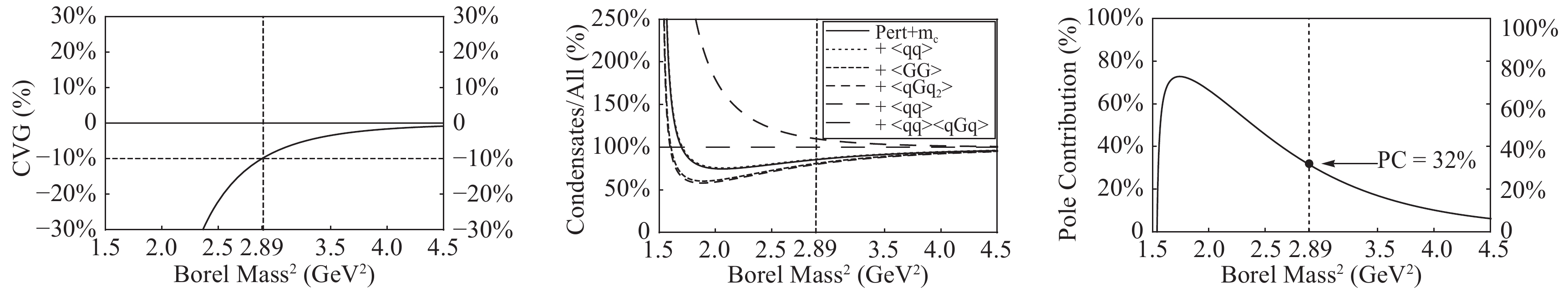
Figure 1. The left panel shows CVG, defined in Eq. (19), as a function of Borel mass
${ M_B }$ . The middle panel shows the relative contribution of each term on the OPE expansion, as a function of Borel mass${ M_B }$ . Right panel shows the variation of PC, defined in Eq. (20), as a function of Borel mass${ M_B }$ . Here we use the current${ J_{\mu,3/2-} }$ of${ J^P = 3/2^- }$ , and choose${ \theta_1=-42^\circ }$ and${ s_0 = 23 }$ GeV2.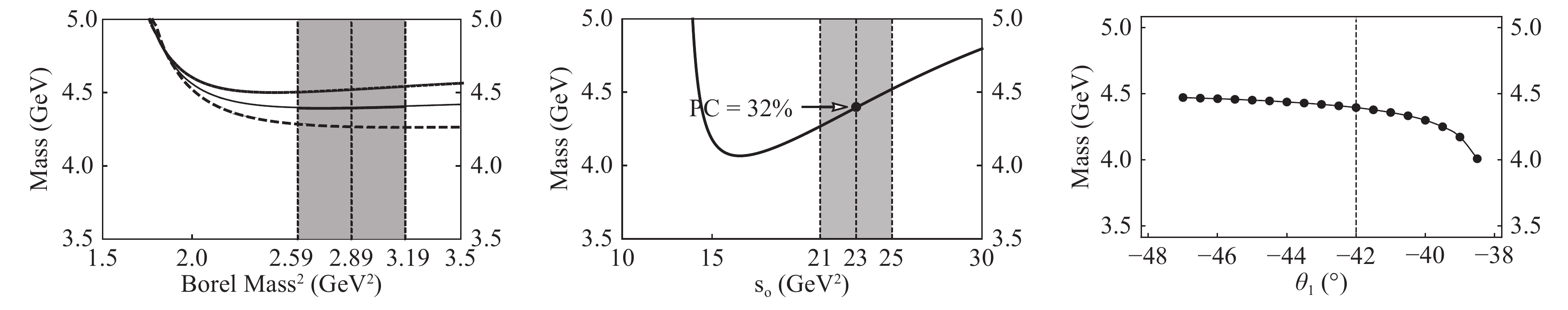
Figure 2. Variations of
${ M_{3/2^-} }$ with respect to Borel mass${ M_B }$ (left), threshold value${ s_0 }$ (middle), and mixing angle${ \theta_1 }$ (right), calculated using the current${ J_{\mu,3/2-} }$ of${ J^P = 3/2^- }$ . In the left panel, the long-dashed, solid, and short-dashed curves are obtained with${ \theta_1=-42^\circ }$ and for${ s_0 }$ = 21, 23, and 25 GeV2, respectively. In the middle figure, the curve is obtained with${ \theta_1=-42^\circ }$ and${ M_B^2 = 2.89 }$ GeV2. In the right figure, the curve is obtained for${ s_0 = 23 }$ GeV2 and with${ M_B }$ satisfying CVG=10%.To use the third criterion to determine
$ s_0 $ , we show variations of$ M_X $ with respect to$ s_0 $ in the middle panel of Fig. 2, with$ \theta_1=-42^\circ $ . The mass curves have a minimum against$ s_0 $ when$ s_0 $ is approximately 17 GeV2; therefore, the$ s_0 $ dependence of the mass prediction is the weakest at this point. However, the PC at this point is significantly small (only 8%). We find that the PC = 32% at$ s_0 = 23 $ GeV2. Moreover, the$ M_B $ dependence is the weakest at this point. Accordingly, we fix the threshold value to be$ s_0 = 23 $ GeV2 and choose 21 GeV2$ \leqslant s_0\leqslant $ 25 GeV2 as our working region.Finally, we vary
$ \theta_1 $ and repeat the above processes. We show variations of$ M_X $ with respect to$ \theta_1 $ in the right panel of Fig. 2 with$ s_0= 23 $ GeV2 and choosing$ M_B $ to satisfy CVG = 10%. We find that the$ \theta_1 $ -dependence of the mass prediction is weak when$ \theta_1 \leqslant -40^\circ $ . Accordingly, we fix the mixing angle$ \theta_1 $ to be$ -42^\circ $ and choose$ \theta_1 = -42\pm5^\circ $ as our working region.For current
$ J_{\mu, 3/2-} $ , we fine-tune the mixing angle$ \theta_1 $ to be −42°, and the working regions are found to be 21 GeV 2$ \leqslant s_0\leqslant $ 25 GeV2 and 2.59 GeV2<$ M_B^2 $ <3.19 GeV2. We assume the uncertainty of$ \theta_1 $ to be −42±5°, and we obtain the following numerical results:$ \begin{split} M_{3/2^-} =& 4.40^{+0.17}_{-0.22} {\rm{ GeV}}, \\ f_{3/2^-} =& \left(6.5^{+3.2}_{-2.9}\right) \times 10^{-4} {\rm{ GeV}}^6, \end{split} $

(21) where the central value corresponds to
$ \theta_1 = -42^\circ $ ,$ s_0 = 23 $ GeV2, and$ M_B^2=2.89 $ GeV2. The mass uncertainty is due to the mixing angle$ \theta_1 $ , Borel mass$ M_B $ , threshold value$ s_0 $ , charm quark mass$ m_c $ , and various condensates [1, 69-76]. We note the following: a) when calculating the mass uncertainty due to the mixing angle$ \theta_1 $ , we have fixed$ s_0 $ and$ M_B $ ; and b) when plotting the mass variation as a function of$ \theta_1 $ , as shown in the right panel of Fig. 2, we have fixed$ s_0 $ , but while choosing$ M_B $ to satisfy CVG = 10%. The above mass value is consistent with the experimental mass of the$ P_c(4380) $ [2], and supports it to be a hidden-charm pentaquark having$ J^P=3/2^- $ . The current$ J_{\mu, 3/2-} $ consists of$ \xi_{36\mu} $ and$ \psi_{9\mu\nu} $ , suggesting that the$ P_c(4380) $ may contain the S-wave$ [\Lambda_c(1P)\bar D_1] $ , P-wave$ [\Lambda_c(1P)\bar D] $ , P-wave$ [\Lambda_c\bar D_1] $ , D-wave$ [\Lambda_c\bar D] $ , S-wave$ [\Sigma_c \bar D^*] $ components, etc.Similarly, we investigate the current
$ J_{\mu\nu, 5/2+} $ of$ J^P = 5/2^+ $ . We fine-tune the mixing angle$ \theta_2 $ to be -45±5°, and the working regions are found to be 21 GeV2$\leqslant s_0\leqslant $ 25 GeV2 and 2.31 GeV2<$ M_B^2 $ <2.91 GeV2. We show the variations of$ M_X $ with respect to$ M_B $ ,$ s_0 $ , and$ \theta_2 $ in Fig. 3, and we obtain the following numerical results: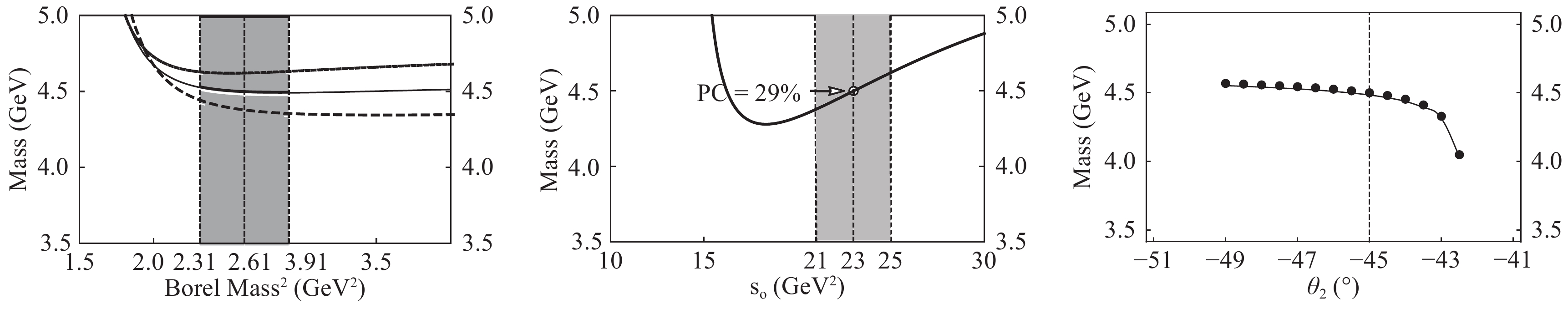
Figure 3. Variations of
${ M_{5/2^+} }$ with respect to the Borel mass${ M_B }$ (left), threshold value${ s_0 }$ (middle), and mixing angle${ \theta_2 }$ (right), calculated using the current${ J_{\mu\nu,5/2+} }$ of${ J^P = 5/2^+ }$ . In the left figure, the long-dashed, solid, and short-dashed curves are obtained with${ \theta_2=-45^\circ }$ and for${ s_0 }$ =21, 23 and 25 GeV2, respectively. In the middle figure, the curve is obtained with${ \theta_2=-45^\circ }$ and${ M_B^2 = 2.61 }$ GeV2. In the right figure, the curve is obtained for${ s_0 = 23 }$ GeV2 and with${ M_B }$ satisfying CVG=10%.$ \begin{split} M_{5/2^+} =& 4.50^{+0.26}_{-0.24} {\rm{ GeV}}, \\ f_{5/2^+} =& \left(5.5^{+3.4}_{-2.4}\right) \times 10^{-4} {\rm{ GeV}}^6, \end{split} $

(22) where the central value corresponds to
$ \theta_2=-45^\circ $ ,$ s_0 = 23 $ GeV2, and$ M_B^2=2.61 $ GeV2. The above mass value is consistent with the experimental mass of the$ P_c(4450) $ [2], and supports it to be a hidden-charm pentaquark having$ J^P=5/2^+ $ . The current$ J_{\mu\nu, 5/2+} $ consists of$ \xi_{15\mu} $ and$ \psi_{4\mu\nu} $ , suggesting that the$ P_c(4450) $ may contain the S-wave$ [\Lambda_c(1P)\bar D^*] $ , P-wave$ [\Lambda_c\bar D^*] $ , S-wave$ [\Sigma_c^* \bar D_1] $ , P-wave$ [\Sigma_c^* \bar D] $ components, etc. -
In this section we follow the same approach to study the hidden-charm pentaquark states of
$ J^P = 3/2^+ $ and$ J^P = 5/2^- $ . We find the following two currents$ \begin{split} J_{\mu, 3/2+} =& \cos\theta_3 \times \xi_{35\mu} + \sin\theta_3 \times \psi_{10\mu} \\ =& \cos\theta_3 \times [\epsilon^{abc} (u^T_a C \gamma_\nu \gamma_5 d_b) \gamma_\nu \gamma_5 c_c] [\bar c_d \gamma_\mu u_d] \\ & + \sin\theta_3 \times [\epsilon^{abc} (u^T_a C \gamma_\nu u_b) \gamma_\nu \gamma_5 c_c] [\bar c_d \gamma_\mu \gamma_5 d_d], \end{split} $

(23) $ \begin{split} J_{\mu\nu, 5/2-} =& \cos\theta_4 \times \xi_{16\mu\nu} + \sin\theta_4 \times \psi_{3\mu\nu} \\ =& \cos\theta_4 \times [\epsilon^{abc} (u^T_a C \gamma_\mu \gamma_5 d_b) c_c] [\bar c_d \gamma_\nu \gamma_5 u_d] \\ & + \sin\theta_4 \times [\epsilon^{abc} (u^T_a C \gamma_\mu u_b) c_c] [\bar c_d \gamma_\nu d_d] \\ & + \{ \mu \leftrightarrow \nu \}, \end{split} $

(24) which have structures similar to
$ J_{\mu, 3/2-} $ and$ J_{\mu\nu, 5/2+} $ , respectively. The extracted spectral densities are also similar to previous results:$ \begin{split} \rho_{3/2+, 1}(s) =& \rho^{\rm pert}_{3/2-, 1}(s) - \rho^{\langle\bar qq\rangle}_{3/2-, 1}(s) + \rho^{\langle GG\rangle}_{3/2-, 1}(s) \\ &- \rho^{\langle\bar qq\rangle^2}_{3/2-, 1}(s) + \rho^{\langle\bar qGq\rangle}_{3/2-, 1}(s) + \rho^{\langle\bar qq\rangle\langle\bar qGq\rangle}_{3/2-, 1}(s), \end{split} $

(25) $ \begin{split} \rho_{5/2-, 1}(s) =& \rho^{\rm pert}_{5/2+, 1}(s) - \rho^{\langle\bar qq\rangle}_{5/2+, 1}(s) + \rho^{\langle GG\rangle}_{5/2+, 1}(s) \\ & - \rho^{\langle\bar qq\rangle^2}_{5/2+, 1}(s) + \rho^{\langle\bar qGq\rangle}_{5/2+, 1}(s) + \rho^{\langle\bar qq\rangle\langle\bar qGq\rangle}_{5/2+, 1}(s), \end{split} $

(26) where
$ \rho^{\rm pert}_{3/2-, 1}(s) $ ,$ \rho^{\rm pert}_{5/2+, 1}(s) $ , and others have been defined in Eqs. (13) and (15).First, we study the current
$ J_{\mu, 3/2+} $ of$ J^P = 3/2+ $ . With the same mixing angle$ \theta_1 $ , i.e.,$ \theta_3 = \theta_1 = -42\pm5^\circ $ , the working regions are found to be 21 GeV2$ \leqslant s_0\leqslant $ 25 GeV2 and 2.58 GeV2<$ M_B^2 $ <3.18 GeV2. We show the variations of$ M_X $ with respect to$ s_0 $ in the left panel of Fig. 4 with$ \theta_3=-42^\circ $ , where the mass is extracted to be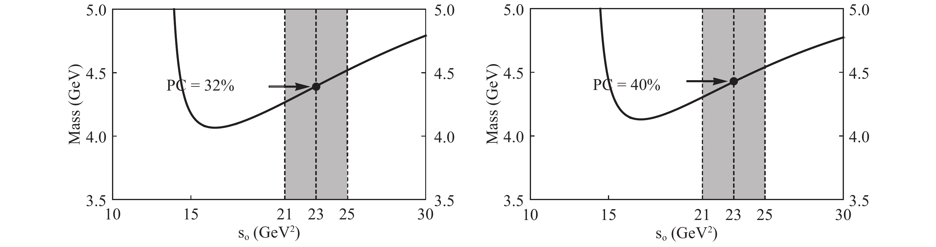
Figure 4. Variations of
${ M_{3/2^+} }$ (left) and${ M_{5/2^-} }$ (right) with respect to the threshold value${ s_0 }$ , calculated using the current${ J_{\mu,3/2+} }$ with${ \theta_3=-42^\circ }$ and${ J_{\mu\nu,5/2-} }$ with${ \theta_4=-45^\circ }$ , respectively.$ M_{3/2^+} = 4.40^{+0.14}_{-0.16} {\rm{ GeV}} . $

(27) Then, we study the current
$ J_{\mu\nu, 5/2-} $ of$ J^P = 5/2- $ . With the same mixing angle$ \theta_2 $ , i.e.,$ \theta_4= \theta_2 = -45\pm5^\circ $ , the working regions are found to be 21 GeV2$ \leqslant s_0\leqslant $ 25 GeV2 and 2.20 GeV2<$ M_B^2 $ <2.80 GeV2. We show vthe ariations of$ M_X $ with respect to$ s_0 $ in the right panel of Fig. 4 with$ \theta_4=-45^\circ $ , where the mass is extracted to be$ M_{5/2^-} = 4.43^{+0.26}_{-0.28} {\rm{ GeV}} . $

(28) The above two values are both consistent with the experimental masses of
$ P_c(4380) $ and$ P_c(4450) $ [2], suggesting that their spin-parity assignments can be different from$ J^P=3/2^- $ and$ 5/2^+ $ , and further theoretical and experimental efforts are required to clarify their properties. -
In this study, we used the method of QCD sum rules to study the hidden-charm pentaquark states
$ P_c(4380) $ and$ P_c(4450) $ . We achieved better QCD sum rule results by requiring the PC to be greater than or equal to 30% in order to ensure that the one-pole parametrization was valid; this criterion is stricter than the one used in our previous studies [57, 58]. We found two mixing currents,$ J_{\mu, 3/2-} $ of$ J^P = 3/2^- $ and$ J_{\mu\nu, 5/2+} $ of$ J^P = 5/2^+ $ . We used them to perform the sum rule analyses, and the masses were extracted to be$ \begin{split} M_{3/2^-} =& 4.40^{+0.17}_{-0.22} {\rm{ GeV}}, \\ M_{5/2^+} =& 4.50^{+0.26}_{-0.23} {\rm{ GeV}} . \end{split} $

These values are consistent with the experimental masses of
$ P_c(4380) $ and$ P_c(4450) $ , suggesting that they can be identified as hidden-charm pentaquark states composed of anti-charmed mesons and charmed baryons:$ P_c(4380) $ has$ J^P=3/2^- $ and may contain the S-wave$ [\Lambda_c(1P)\bar D_1] $ , P-wave$ [\Lambda_c(1P)\bar D] $ , P-wave$ [\Lambda_c\bar D_1] $ , D-wave$ [\Lambda_c\bar D] $ , S-wave$ [\Sigma_c \bar D^*] $ components, etc.$ P_c(4450) $ has$ J^P=5/2^+ $ and may contain the S-wave$ [\Lambda_c(1P)\bar D^*] $ , P-wave$ [\Lambda_c\bar D^*] $ , S-wave$ [\Sigma_c^* \bar D_1] $ , P-wave$ [\Sigma_c^* \bar D] $ components, etc.We follow the same approach to study the hidden-charm pentaquark states of
$ J^P = 3/2^+ $ and$ J^P = 5/2^- $ , and extract their masses to be$ \begin{split} M_{3/2^+} =& 4.40^{+0.14}_{-0.16} {\rm{ GeV}}, \\ M_{5/2^-} =& 4.43^{+0.26}_{-0.28} {\rm{ GeV}} . \end{split} $

These values are also consistent with the experimental masses of
$ P_c(4380) $ and$ P_c(4450) $ [2], suggesting that there still exist other possible spin-parity assignments, which should be clarified in further theoretical and experimental studies.We have also investigated the bottom partners of
$ P_c(4380) $ and$ P_c(4450) $ , i.e., the hidden-bottom pentaquark states ($ b \bar b u u d $ ) of$ J^P = 3/2^- $ and$ J^P = 5/2^+ $ . As shown in Fig. 5, their masses are extracted to be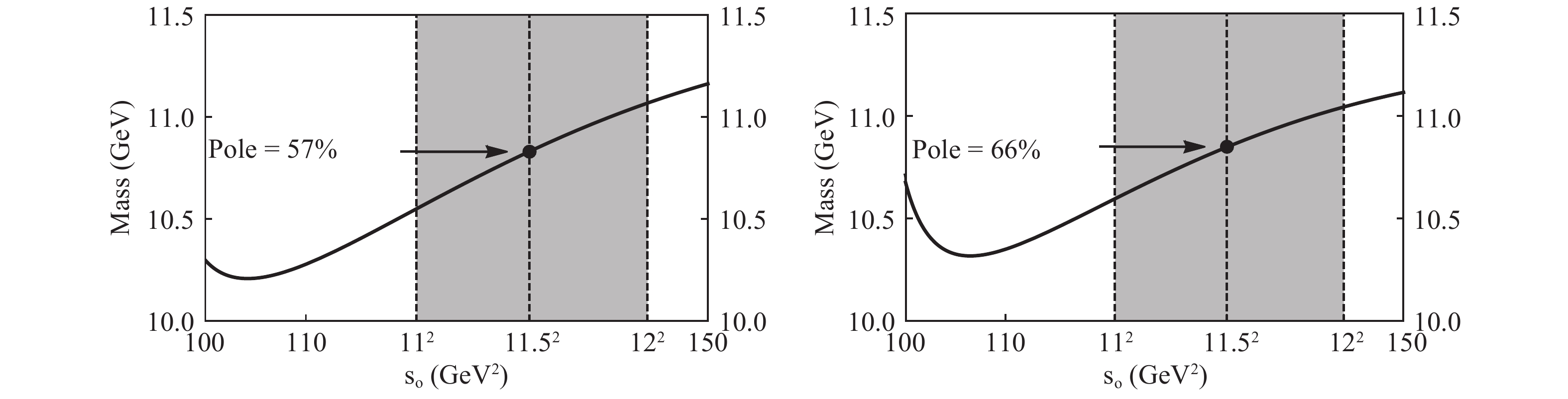
Figure 5. Variations of
${ M_{P_b(3/2^-)} }$ (left) and${ M_{P_b(5/2^+)} }$ (right) with respect to the threshold value${ s_0 }$ , calculated using the current${ J^{b \bar b u u d}_{\mu,3/2-} }$ with${ \theta_1=-42^\circ }$ and${ J^{b \bar b u u d}_{\mu\nu,5/2+} }$ with${ \theta_2=-45^\circ }$ , respectively.$ \begin{split} M_{P_b(3/2^-)} =& 10.83^{+0.26}_{-0.29} {\rm{ GeV}}, \\ M_{P_b(5/2^+)} =& 10.85^{+0.24}_{-0.27} {\rm{ GeV}} . \end{split} $

(29) We propose to search for them in the future LHCb and BelleII experiments.
In conclusion, we note that there are a considerable systematical uncertainties that are not considered in the present study, such as the vacuum saturation for higher dimensional operators, which is used to calculate the OPE . Moreover, in this study, we used the running charm and bottom quark masses in the
$ \overline{MS} $ scheme, while sometimes their pole masses were used. Consider thee current$ J_{\mu, 3/2-} $ as an example: a) if we use$ \langle 0 | \bar q q \bar q q |0 \rangle = ( 0.8 \sim 1.2 ) \times$ $ \langle 0 | \bar q q |0 \rangle \langle 0|\bar q q |0 \rangle $ , we would obtain$ M_{3/2^-} $ =4.34 GeV~4.48 GeV (other uncertainties are not included); b) if we use the pole charm mass$ m_c = 1.67 $ GeV [1], we would have to shift the mixing angle to be approximately$ \theta_1 = -38^\circ $ to arrive at the similar mass$ M_{3/2^-} = 4.38 $ GeV. Combining the previous uncertainties in Eqs. (21), (22), (27), and (28), we obtain the following result for the mixing current$ J_{\mu, 3/2-} $ of$ J^P = 3/2^- $ $ M_{3/2^-} = 4.40^{+0.19}_{-0.23} {\rm{ GeV}} . $

Similarly, we obtain the following results for the other three mixing currents,
$ J_{\mu\nu, 5/2^+} $ of$ J^P = 5/2^+ $ ,$ J_{\mu, 3/2^+} $ of$ J^P = 3/2^+ $ , and$ J_{\mu\nu, 5/2^-} $ of$ J^P = 5/2^- $ :$ \begin{split} M_{5/2^+} =& 4.50^{+0.28}_{-0.27} {\rm{ GeV}}, \\ M_{3/2^+} =& 4.40^{+0.16}_{-0.17} {\rm{ GeV}}, \\ M_{5/2^-} = &4.43^{+0.27}_{-0.29} {\rm{ GeV}} . \end{split} $

The above (systematical) uncertainties are significant, suggesting that we still know little about exotic hadrons, and further experimental and theoretical studies are necessary to understand them well.
We thank Professor Nikolai Kochelev for helpful discussions.
Revisiting hidden-charm pentaquarks from QCD sum rules
- Received Date: 2018-04-16
- Accepted Date: 2018-12-04
- Available Online: 2019-03-01
Abstract: We revisit hidden-charm pentaquark states


 DownLoad: