


 Abstract
 HTML
HTML Reference
 Related
 PDF
PDF


-
Cosmic accelerating expansion is a major discovery. Numerous dynamical mechanisms have been proposed to explain this phenomenon; however, its nature is not understood yet. There are many theories that attempt to account for the accelerating expansion of the universe, such as modified gravity, dark energy, or the violation of cosmological principle. Modified gravity theories do not need any exotic energy-momentum components except the modifications of the general relativity to explain the cosmic acceleration. The expansion of the universe can be quantitatively studied with a variety of cosmological observations. In this field, directly obtaining implications from observational data, without introducing any hypothesis, for the composition of the universe or prior theory of gravity is an important issue.
Gaussian processes (GPs), which are fully Bayesian and describe a distribution over functions, can reconstruct a function from observational data without assuming any parametrization. This algorithm was first proposed to reconstruct dark energy and expansion dynamics [1] and was implemented with a package in Python (GaPP①): Gaussian processes in Python). Later, it was widely used in the literature for cosmography, such as reconstructions of the dark energy equation of state [2-6], expansion history [7-11], cosmic growth and matter perturbations [12-17], tests of the distance duality relation [18-24], cosmic curvature [25-33], tests of the speed of light [34-36], interactions between dark sectors [37, 38], and Hubble constant from cosmic chronometers [39-42]. In these works, by using GaPP, functions of the Hubble parameter with respect to the redshift and the distance-redshift relation were frequently reconstructed from the expansion rate measurements and type Ia supernovae (SNe Ia) observations, respectively. Moreover, derivatives and integrals of these reconstructed functions are further obtained for other implications, such as dark energy evolution, cosmic curvature, and tests for the speed of light. However, the fidelity of GaPP when used for smoothing currently available discrete expansion rate measurements and distance observations has not been verified yet.
In this study, we test the fidelity of GaPP for cosmography by simulating upcoming expansion rate measurements and distance observations with different number of events and uncertainty levels. It is suggested that both factors, sample size and uncertainty level, are crucial to the reliability of GaPP reconstruction. That is, for expansion rate measurements, GaPP reconstruction is valid when ~256 data points with average relative 3% uncertainty level are obtained. Moreover, the distance-redshift relation, reconstructed using GaPP, is credible when the near-future Dark Energy Survey (DES) SNe Ia is considered.
The remainder of this paper is organized as follows. We first briefly introduce GP in Section 2. Next, we describe the method for simulating the data of the Hubble parameter versus redshift, H(z), and SNe Ia from the DES in Section 3. Moreover, we use GP to process mock data sets and results are also presented in Section 3. Finally, in Section 4, we discuss obtained results and provide some conclusions.
-
For a given set of Gaussian distributed observations
$ \{(x_i, y_i)|i=1, 2, ..., n\} $ with${X} $ being the locations of observations, i.e.$ \{x_i\}^n_{i=1} $ , we want to reconstruct the most probable underlying continuous function which describes the data at the test input points${X}^* $ . GP, which makes it possible to achieve this goal, is a distribution over functions and thus, is a generalization of a Gaussian distribution. For a function f formed from a GP, the value of f at x is a Gaussian random variable with mean and variance being$ \mu(x) $ and$ {\rm{Var}}(x) $ , respectively. Moreover, the value of f at x is not independent of the value at some other points$ \tilde{x} $ , but is related by a covariance function,$ {\rm{cov}}(f(x), f(\tilde{x}))=k(x, \tilde{x})=\mathbb{E}[(f(x)-\mu(x))(f(\tilde{x})-\mu(\tilde{x}))]. $

(1) In this case, GP is defined by the mean
$ \mu(x) $ and covariance$ k(x, \tilde{x}) $ ,$ f(x)\sim{\cal{G}}{\cal{P}}[\mu(x), k(x, \tilde{x})]. $

(2) For each
$ x_i $ , the value of f, i.e.,$ f(x_i) $ , is derived from a Gaussian distribution with mean$ \mu(x_i) $ and variance$ k(x_i, x_i) $ . In addition,$ f(x_i) $ correlates with$ f(x_j) $ via the covariance function$ k(x_i, x_j) $ .Choosing a suitable covariance function is essential for satisfactory reconstruction. It is common to select a squared exponential function for the covariance function,
$ k(x,\tilde x) = \sigma _f^2\exp \left[ { - \frac{{{{(x - \tilde x)}^2}}}{{2{\ell ^2}}}} \right], $

(3) where
$ \sigma_f $ is the hyperparameter that describes the typical change in y direction,$ \ell $ is another hyperparameter that characterizes the length scale and can be considered as the distance moving in input space before the function value changes significantly. These two hyperparameters, in contrast to the actual parameters, do not specify the exact formula of a function, but represent typical changes in the function value. This function has the advantage that it is infinitely differentiable and therefore, is useful for reconstructing the derivative of a smoothed function.For
${X}^* $ , the covariance matrix is given by${[K({{{X}}^*}, {{{X}}^*})]_{ij}} = k(x_i^*, x_j^*)$ . Then the vector${f}^* $ with entries$ f(x^*_i) $ can be obtained from a Gaussian distribution:$ {{{f}}^*} \sim N(\mu ({{{X}}^*}), K({{{X}}^*}, {{{X}}^*})). $

(4) This distribution can be considered as a prior of
${f}^* $ , and observational information is necessary to obtain the posterior distribution. For uncorrelated observational data, its covariance matrix C is diagonal with entries$ \sigma_i $ . Then the combined distribution for observations y and${f}^* $ is given by$ \left[{\begin{array}{*{20}{c}} {{y}}\\ {{{{f}}^*}} \end{array}} \right] \sim N\left( {\left[{\begin{array}{*{20}{c}} \mu \\ {{\mu ^{\rm{*}}}} \end{array}} \right], \left[{\begin{array}{*{20}{c}} {K({{X}}, {{X}}) + C} & {K({{X}}, {{{X}}^*})}\\ {K({{{X}}^*}, {{X}})} & {K({{{X}}^*}, {{{X}}^*})} \end{array}} \right]} \right). $

(5) Here, we are interested in the conditional distribution,
$ {{{f}}^*}|{{{X}}^*}, {{X}}, {{y}} \sim N\left( {{{\overline {{f}} }^*}, {\rm{cov}}({{{f}}^*})} \right), $

(6) because the values of y are already known, and we want to reconstruct
${f}^* $ . Moreover,$ {\overline {{f}} ^*} = {\mu ^{\rm{*}}}{\rm{ + }}K({{{X}}^{\rm{*}}}, {{X}}){\left[{K({{X}}, {{X}}){\rm{ + C}}} \right]^{{\rm{ - 1}}}}({{y}}{\rm{ - }}\mu ) $

(7) and
$ {\rm{cov}}({{{f}}^*}) = K({{{X}}^*}, {{{X}}^*}) - K({{{X}}^*}, {{X}}){\left[{K({{X}}, {{X}}) + C} \right]^{ - 1}}K({{X}}, {{{X}}^*}), $

(8) are the mean and covariance of
${f}^* $ , respectively. Before using Eq. (6), to obtain the posterior distribution of the function for the given data and prior (Eq. (4)), we have to obtain the values of the hyperparameters$ \sigma_f $ and$ \ell $ , which can be trained by maximizing the following marginal likelihood:$ \begin{split} \ln L =& \ln p({{y}}|{{X}}, {\sigma _f}, \ell )\\ =& - \displaystyle\frac{1}{2}{({{y}} - \mu )^ \top }{\left[{K({{X}}, {{X}}) + C} \right]^{ - 1}}({{y}} - \mu )\\ &- \displaystyle\frac{1}{2}\ln \left| {K({{X}}, {{X}}) + C} \right| - \displaystyle\frac{n}{2}\ln 2\pi . \end{split} $

(9) This likelihood is only dependent on the observational data
$ \{(x_i, y_i)|i=1, 2, ..., n\} $ but free of the locations${X}^* $ where the function is to be reconstructed. Refer to Ref. [1] for a more detailed analysis and description of the GP. GaPP (GP in Python) is a popular package in Python to reconstruct a function from observational data. -
In this work, we simulated data sets to test the fidelity of GaPP because the assumed fiducial model for simulations is known. To generate simulated H(z) data sets, three issues must be addressed: i) the number of future data points; ii) redshift distribution of observed events in the near future; iii) possible uncertainty levels of upcoming observations. We individually expound these three aspects in detail in the following analysis.
-
For the number of events in simulations, we consider the cases with 64, 128, and 256 data points. These numbers are chosen because the constraining power of 64 H(z) measurements with the same quality as today is comparable with that of current SNe Ia [43]. For redshifts of observed events in the near future, we assume that they will trace the distribution of redshifts of currently available H(z) measurements compiled in [26]. The histogram of the number of observed expansion rates is plotted in Fig. 1. We fit the histogram with a gamma distribution, and the result is denoted by a solid red line in this plot. For possible uncertainty levels, we first assume that future data will provide measurements with the same errors as the existing observations. In this case, we update the approach in [43] to predict future data based on recent measurements. The general trend of errors increasing with redshift z appears as we show uncertainties on H(z) in Fig. 2. Moreover, we observe that, besides two outliers at z= 0.48 and z= 0.88, uncertainties
$ \sigma(z) $ are confined in the region between the lines$ \sigma_+\!=\!20.50z\!+\!10.17 $ and$ \sigma_-=8.292z-0.53 $ . It is expected that the mean uncertainty of future observations follows the meanline of the strip$ \sigma_0=14.71z+4.82 $ . Then we draw a random variable$ \tilde{\sigma}(z) $ from the Gaussian distribution$ N(\sigma_0(z), \varepsilon(z)) $ as the error of the simulated point. Here, the parameter$ \varepsilon(z)=(\sigma_+-\sigma_-)/4 $ is set to assure that the error$ \tilde{\sigma}(z) $ falls in the region with a 95.4% probability. In addition to the current quality, we also consider some other smaller errors for simulated H(z) data sets of relative 10%, 5%, and 3% levels [44]. In their analysis, it was found that, for extended scenarios of star formation history, H(z) can be recovered to 3% by selecting galaxies from the Millennium simulation and using rest-frame criteria, which significantly improves the homogeneity of the sample.
Figure 1. (color online) Histogram of 28 currently available measurements of expansion rate with respect to redshift, H(z). The solid red curve is plotted assuming a gamma distribution to match the number of observational events.

Figure 2. (color online) Uncertainties of 28 currently measured H(z). Solid dots and empty circles are nonoutliers and outliers, respectively. Bounds σ+ and σ− are plotted as red dashed lines. The mean uncertainty σ0 is shown as the black solid line.
After addressing the aforementioned three issues, we can generate a simulated H(z) point in a given fiducial model. First, the fiducial value
$ H_{\rm{fid}}(z) $ is obtained from the spatially flat$ \Lambda $ CDM model$ H_{\rm{fid}}(z)= H_0\sqrt{\Omega_m(1+z)^3+1-\Omega_m}, $

(10) with
$ H_0 = 67.74 $ and$ \Omega_m = 0.31 $ [45]. Next, a random number satisfying the Gaussian distribution$ N(\sigma_0(z), \varepsilon(z)) $ is drawn as the uncertainty$ \tilde{\sigma}(z) $ . This quantity is also used to obtain the deviation of the simulated data point from the fiducial one,$ \Delta H=H_{\rm{sim}}(z)-H_{\rm{fid}}(z) $ , which is subject to the Gaussian distribution$ N(0, \tilde{\sigma}(z)) $ . Finally, a mock data point$ H_{\rm{sim}}(z)=H_{\rm{fid}}(z)+\Delta H $ is generated, with its corresponding uncertainty$ \tilde{\sigma}(z) $ .Simulated data sets including 64, 128, and 256 points with various levels of uncertainty are shown in Figs. 3-5. Moreover, we use the GaPP to reconstruct the functions of the Hubble parameter vs. redshift. The results (shaded red regions) are presented in the corresponding figures. In addition to these simulations and reconstructions for expansion rate measurements, we also mock distance data set of SNe Ia based on the upcoming DES [46]. The simulated data and reconstructed distance-redshift relation are shown in Fig. 6.

Figure 3. (color online) Simulated 64 events of expansion rates with different uncertainty levels and the functions of Hubble parameter vs. redshift (shaded red regions) reconstructed from the mock data with the GaPP.
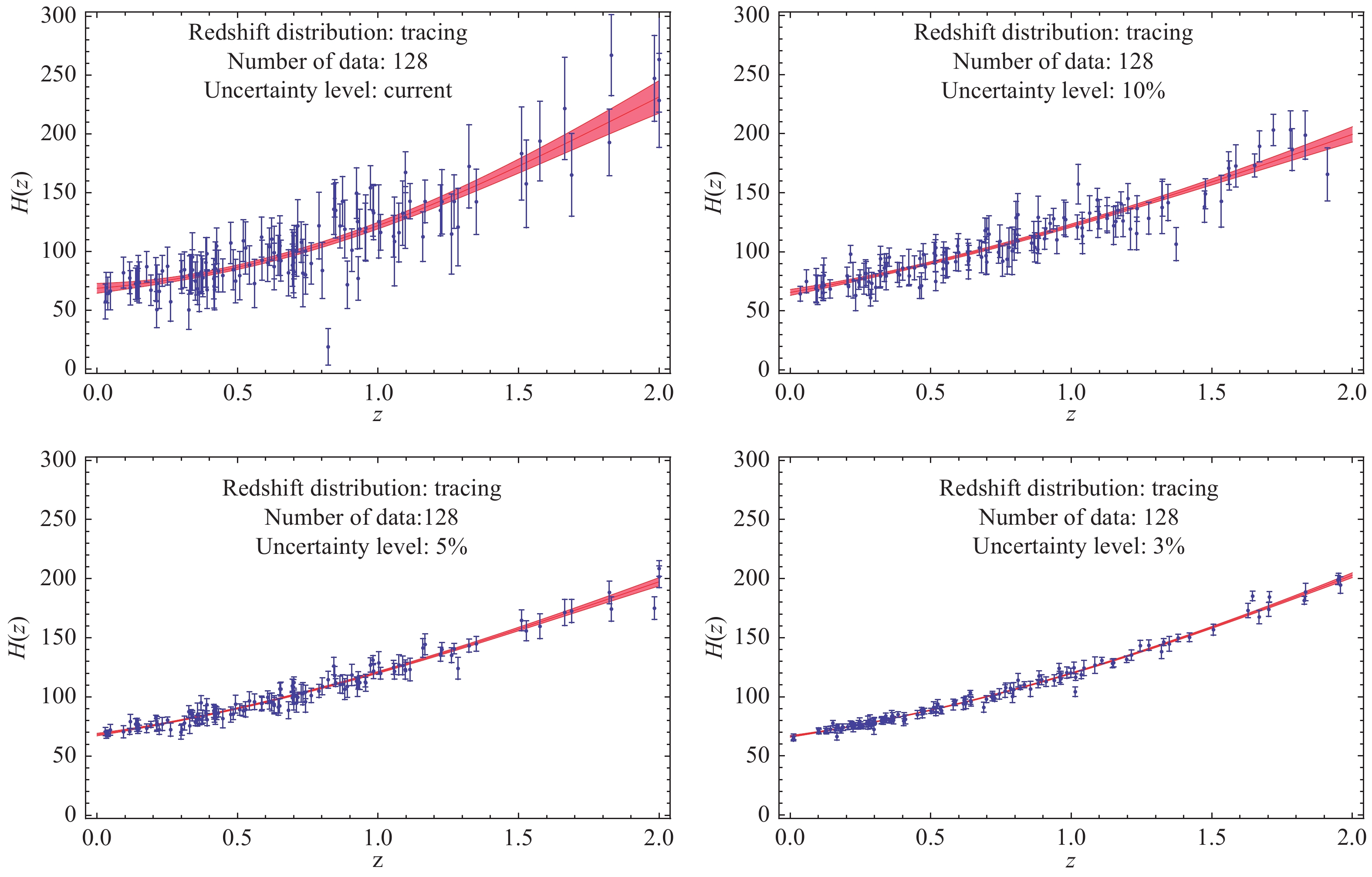
Figure 4. (color online) Simulated 128 events of expansion rates with different uncertainty levels and the functions of Hubble parameter vs. redshift (shaded red regions) reconstructed from the mock data with the GaPP.

Figure 5. (color online) Simulated 256 events of expansion rates with different uncertainty levels and the functions of Hubble parameter vs. redshift (shaded red regions) reconstructed from the mock data with the GaPP.
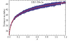
Figure 6. (color online) Simulated ~4000 distance estimations from the upcoming DES SNe Ia observations and the distance-redshift relation (shaded red region) reconstructed from the mock data with the GaPP.
-
To test the fidelity of the GaPP, we appeal to the residual of the fiducial model on which simulations are based and the function reconstructed from the corresponding mock data to characterize the deviation between them. Results related to this quantity for both simulations of expansion rate measurements and distance observations are presented in Figs. 7-9. In our analysis, it is almost certain that the GaPP is less invalid as differences of the reconstructed function from the true model deviate significantly from the horizontal line (Residual = 0). For the Hubble parameter vs. redshift, as suggested in these plots, the validity of the GaPP increases with an increase in the number of simulated data points. On the contrary, the uncertainty level of mock data is also crucial for the fidelity of reconstruction. That is, the GaPP is more valid for reconstructing data with smaller relative uncertainties. In particular, as indicated from the upper-left panel of Fig. 7 for the mock data including 64 points with the current quality, the GaPP reconstruction significantly deviates from the fiducial model. For the case of 128 points with 3% relative uncertainty (the lower-right panel of Fig. 8), the reconstructed function is in good agreement with the fiducial model. Moreover, from the lower-right panel of Fig. 9, we find that the GaPP reconstruction is perfectly consistent with the fiducial scenario at
$ 1\sigma $ confidence level when the dataset containing 256 events with a relative 3% uncertainty is considered. For ~4000 forthcoming distance estimations of DES SNe Ia, except for the range z<0.2, the reconstructed distance-relation is very close to the one in the fiducial model (as shown inFig. 10). This is because, according to the DES program, there are only a small amount of SNe Ia to be observed in the redshift range z<0.2.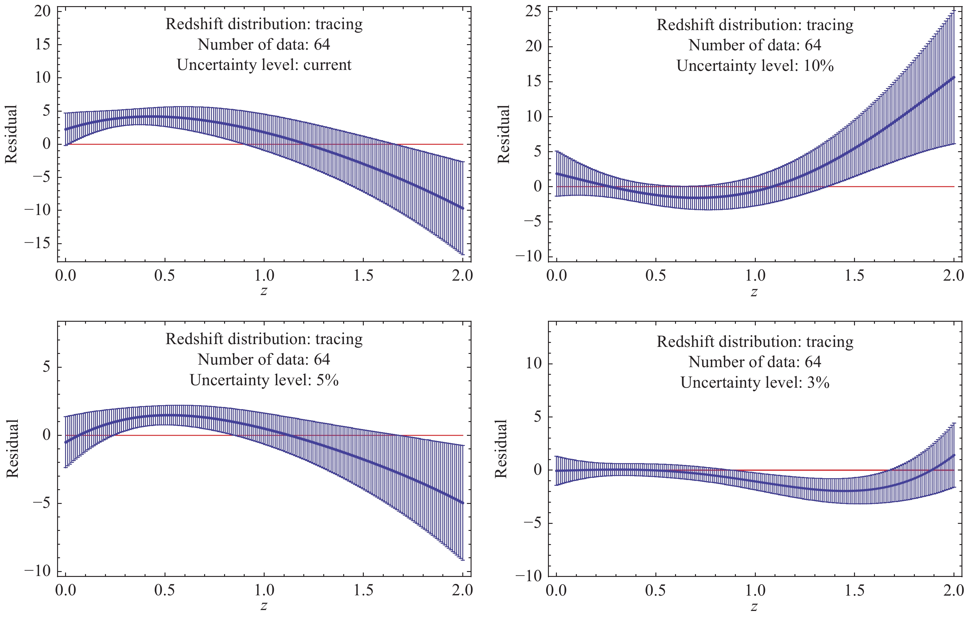
Figure 7. (color online) Residuals between the reconstructed functions of Hubble parameter with respect to redshift and the fiducial model when samples including 64 simulated events with various uncertainty levels are considered.

Figure 8. (color online) Residuals between the reconstructed functions of Hubble parameter with respect to redshift and the fiducial model when samples including 128 simulated events with various uncertainty levels are considered.

Figure 9. (color online) Residuals between the reconstructed functions of Hubble parameter with respect to redshift and the fiducial model when samples including 256 simulated events with various uncertainty levels are considered.

Figure 10. (color online) Residual between the reconstructed functions of distance with respect to redshift and the fiducial model when the upcoming DES SN Ia including ~4000 simulated events is considered.
-
In this work, we use the simulated Hubble parameter and distance vs. redshift data sets to test the fidelity of the GaPP for cosmography. For mock H(z) measurements, we consider data sets including different number of points (64, 128, and 256) with various uncertainty levels (current quality, 10%, 5%, and 3%). As expected, using the residual between the fiducial model for generating mock data and the reconstructed function from it with the GaPP to characterize the fidelity, we find that both the sample size and precision are crucial for the reliability of the GaPP when it is used for reconstructing the function of the Hubble parameter with respect to the redshift from the simulated H(z) data. On one hand, for the data set containing 64 points with the same uncertainty as today, significant deviation between the reconstructed function and the fiducial model suggests that the GaPP might be unreliable to smoothen currently available H(z) measurements for cosmography. On the other hand, the reconstructed function with the GaPP is extremely consistent with the fiducial model when the data set containing 256 points with a relative 3% uncertainty is considered. It implies that the GaPP reconstruction of H(z) data for cosmography is reliable at a very high confidence level. For simulated data of distances, we consider distance estimations of SNe Ia on the basis of DES and obtain that, except for the range z<0.2, there is no obvious deviation of the reconstructed distance-redshift relation from the one in the fiducial model. That is, the GaPP is almost valid for reconstructing the function of distance vs. redshift from DES SNe Ia observations.
Testing the fidelity of Gaussian processes for cosmography
- Received Date: 2018-11-28
- Available Online: 2019-03-01
Abstract: The dependence of implications from observations on cosmological models is an intractable problem not only in cosmology, but also in astrophysics. Gaussian processes (GPs), a powerful nonlinear interpolating tool without assuming a model or parametrization, have been widely used to directly reconstruct functions from observational data (e.g., expansion rate and distance measurements) for cosmography. However, the fidelity of this reconstructing method has never been checked. In this study, we test the fidelity of GPs for cosmography by mocking observational data sets comprising different number of events with various uncertainty levels. These factors are of great importance for the fidelity of reconstruction. That is, for the expansion rate measurements, GPs are valid for reconstructing the functions of the Hubble parameter versus redshift when the number of observed events is as many as 256 and the uncertainty of the data is ~ 3%. Moreover, the distance-redshift relation reconstructed from the observations of the upcoming Dark Energy Survey type Ia supernovae is credible.


 DownLoad: