


 Abstract
 HTML
HTML Reference
 Related
 PDF
PDF


-
The cosmological principle implies that the Universe is homogeneous and isotropic on large scale. This assumption has been verified by many observations, such as the statistical properties of galaxy distribution [1] and of the cosmic microwave background radiation by the Wilkinson Microwave Anisotropy Probe (WMAP) [2, 3] and Planck satellites [4-6]. Based on this principle, the
$ \Lambda $ Cold Dark Matter model ($ \Lambda $ CDM) has been proposed and it is in good agreement with many experiments. However, some observations indicate a possible conflict with the cosmological principle, such as the anisotropy of the cosmic microwave background radiation spectrum [4, 5], the inconsistency of the fine structure constants from the observations of the north and south celestial spheres [7-10], the existence of cosmological preferred direction of rotationally supported galaxies [11, 12], the MOND acceleration scale which is inconsistent with isotropic universe [13], and the anisotropy of the relation between distance and redshift given by the type-Ia supernovae [14-18]. These observations strongly suggest that there may exist a tiny anisotropy in the Universe. If the Universe is really anisotropic, there should be new physics beyond the standard cosmological model.It is natural to study cosmological anisotropy using the relation between the luminosity distance and redshift. The recently observed gravitational waves (GW) [19, 20] provide a new way of observing luminosity distances independent of cosmological models. GW is self-calibrating. The luminosity distance of the GW source can be obtained just from the GW signal. If the GW signal has an electromagnetic counterpart, the redshift of the GW source can be measured by its electromagnetic counterpart.
GW170817, a breakthrough in the history of GW observations, is a signal of a merging binary neutron star (BNS). Its electromagnetic counterpart showed that the source is located at NGC4993 (
$ z\sim 0.01 $ ). The luminosity distance is given by the GW signal [20]. The aLIGO&Virgo collaborations used these data to constrain the Hubble constant and gave the result of$ H_0 = 70.0^{+ 12.0}_{- 8.0}\; \rm{km\; s^{-1}\; Mpc^{-1}} $ [21]. This implies that GW is a very powerful tool for constraining cosmological parameters. In this paper, we study the possibility of constraining the anisotropy of space-time using GW.We note that compared to the detectors which are expected to be built in the future, aLIGO&Virgo is not very powerful [22]. It can only detect a BNS merging event with about
$ z<0.05 $ [23, 24]. Thus, we consider the third generation GW detector, the Einstein Telescope (ET) [25]. ET is a GW detector that is still in the conceptual phase, which will have in one possible design [26], three arms at an angle of 60 degrees to each other, providing the ability to detect signals with$ z \sim 1 $ for BNS merging events . The main purpose of this paper is to investigate the possibility of constraining the anisotropy of the Universe using ET.It should be noted that the Fisher matrix has been used to constrain cosmological parameters [27-30]. There is no doubt that the Fisher matrix is a powerful tool for reaching the uncertainty of parameters of a model in future observations, as it can give the lower limit of the uncertainty of model parameters. However, this lower limit can only be achieved when all system and instrumental errors are considered and best data processing is used. In the actual GW detection, data processing is very complicated, and it can not be guaranteed that the lower limit of the uncertainty given by the Fisher matrix is obtained. In this paper, we use a new way to predict the uncertainty. We get the GW waveform by simulating the BNS merging events, and use the GW waveform and the noise of the GW detectors to obtain the simulated signals. Markov-Chain Monte-Carlo (MCMC) is employed to infer the cosmological parameters from the simulated signals. This procedure completely simulates the real GW signal processing. We use the results of Planck 2015 as fiducial parameters for the standard cosmology model [5]. Bilby [31] is employed as the signal injection and parameter inference tool.
The rest of the paper is organized as follows. In Section 2, we simulate the GW signals and make parameter inferences to obtain the uncertainty of the luminosity distance. In Section 3, we constrain the anisotropy of the Universe by making use of the simulated GW. Section 4 is devoted to the concluding remarks.
-
Gravitational waves are fluctuations of the space-time metric. Standard siren is a GW event for which both the GW and corresponding electromagnetic signals are observed. The observed GW170817 is such a BNS merging event [20].
GW generated by the BNS merging event at the inspiral stage can be roughly described by the post-Newton (PN) approximation. Here, we use the TaylorF2 model, which is also currently used by aLIGO&Virgo [32]. The TaylorF2 model is a purely analytic PN model. It includes point-particle and aligned-spin terms to 3.5PN order, as well as leading order (5PN) and next-to-leading-order (6PN) tidal effects [33]. There are several parameters in this model that affect the waveform of a GW propagating to Earth: the masses, spins, tidal deformability parameters of the two stars, the luminosity distance of the source, the inclination angle between the two stars angular momentum and our sight, the sky position of the source, the time that GW propagates to the geocentric, and the initial phase and the polarization angle.
For convenience, we take here the following values of the parameters:
- The mass of the two neutron stars is
$ 1.4M_{\odot} $ .$ 1.4M_{\odot} $ is a typical neutron star mass.- We assume the neutron stars to be spinless, because we usually consider that stars in a binary system are old neutron stars. If the period of spin is much larger than the period of revolution, the spin effect can be ignored. Refs. [34-36] suggested that radio observable pulsars in BNS have a distribution of spin periods that extends down to about 15 ms.
- We assume that the angular momentum of BNS is in line with our line of sight. This is because the electromagnetic radiation generated in the event of BNS merger is along the direction of the orbital momentum. If the direction were inconsistent with our line of sight, we would not be able to observe the electromagnetic signal [37].
- The GW events are homogeneously distributed on the celestial sphere.
- The luminosity distance is described by the fiducial
$ \Lambda $ CDM.- The phase angle is homogeneously distributed in (0, 2
$ \pi $ ).- The polarization angle is homogeneously distributed in (0,
$ \pi $ ).- We assume a homogeneous distribution of arrival times.
- The dimensionless tidal deformability parameter of the two stars is dependent on the equation of state of the neutron star. However, this parameter has little effect on our result. Referring to Figure 5 of Ref. [20], we take 425 for both neutron stars.
We add the GW signal to the detector noise and then employ MCMC to infer the parameters. For parameter inference, we fix the masses, spins, angular momentum direction, sky position of the source (which can be accurately observed with the electromagnetic signals) and the tidal deformability parameters. Only the remaining four parameters need to be inferred, i.e.
$({d_L},\phi ,\varphi ,{t_0})$ , the luminosity distance, polarization angle, phase and arrival time. We use Bilby [31] for simulation and parameter inference, use dynesty① as the MCMC sampler and set npoints = 5000, dlogz = 0.01.In Ref. [26], it was shown that the horizon of the BNS merging event in ET is expected to reach redshifts of
$ z\sim 1 $ . We choose 10 points in the interval$ z = (0,1) $ with a step size$ \Delta z = 0.02 $ . For each z, we simulate 160 BNS merging events. In each simulation, we use the standard cosmological model to calculate the luminosity distance, and take homogeneously the direction ($ l,b $ ), phase, polarization angle and arrival time according to the method described in the previous section. We then employ MCMC to infer the luminosity distance, polarization angle, phase and arrival time. In inferring these parameters, we set the prior of$ d_L $ uniformly distributed in the co-moving volume from 0 to$5{d_{{L_{{\rm{inject}}}}}}$ , where${d_{{L_{{\rm{inject}}}}}}$ is the injected luminosity distance. In the simulation process, only the “GW detectable” BNS events are considered. We deem a BNS event “GW detectable” when the ET network has a signal-to-noise ratio (SNR)$ >8 $ .For a given redshift z, we only use the inferred uncertainty of
$ d_L $ , which has a center value and two uncertainties$ {d_L}^{- \sigma^-_{d_L}}_{+ \sigma^+_{d_L}}\; $ . For convenience, we combine them into${\sigma _{{d_L}^\prime }} = \sqrt {\frac{{{{(\sigma _{{d_L}}^ + )}^2} + {{(\sigma _{{d_L}}^ - )}^2}}}{2}} .$

Thus, we get 160 uncertainties (for high redshfits, as some of their SNR , and the average of the 160
$ \sigma_{d_L}' $ is$\sigma _{{d_L}}^2 = \frac{1}{{\displaystyle\frac{1}{{160}}\displaystyle\sum\nolimits_{i = 1}^{160} {\left( {\frac{1}{{{{\left( {\sigma _{{d_L}i}'} \right)}^2}}}} \right)} }}.$

(1) The uncertainty is the 68% credible interval.
We do the same procedure for all redshifts z, and obtain a
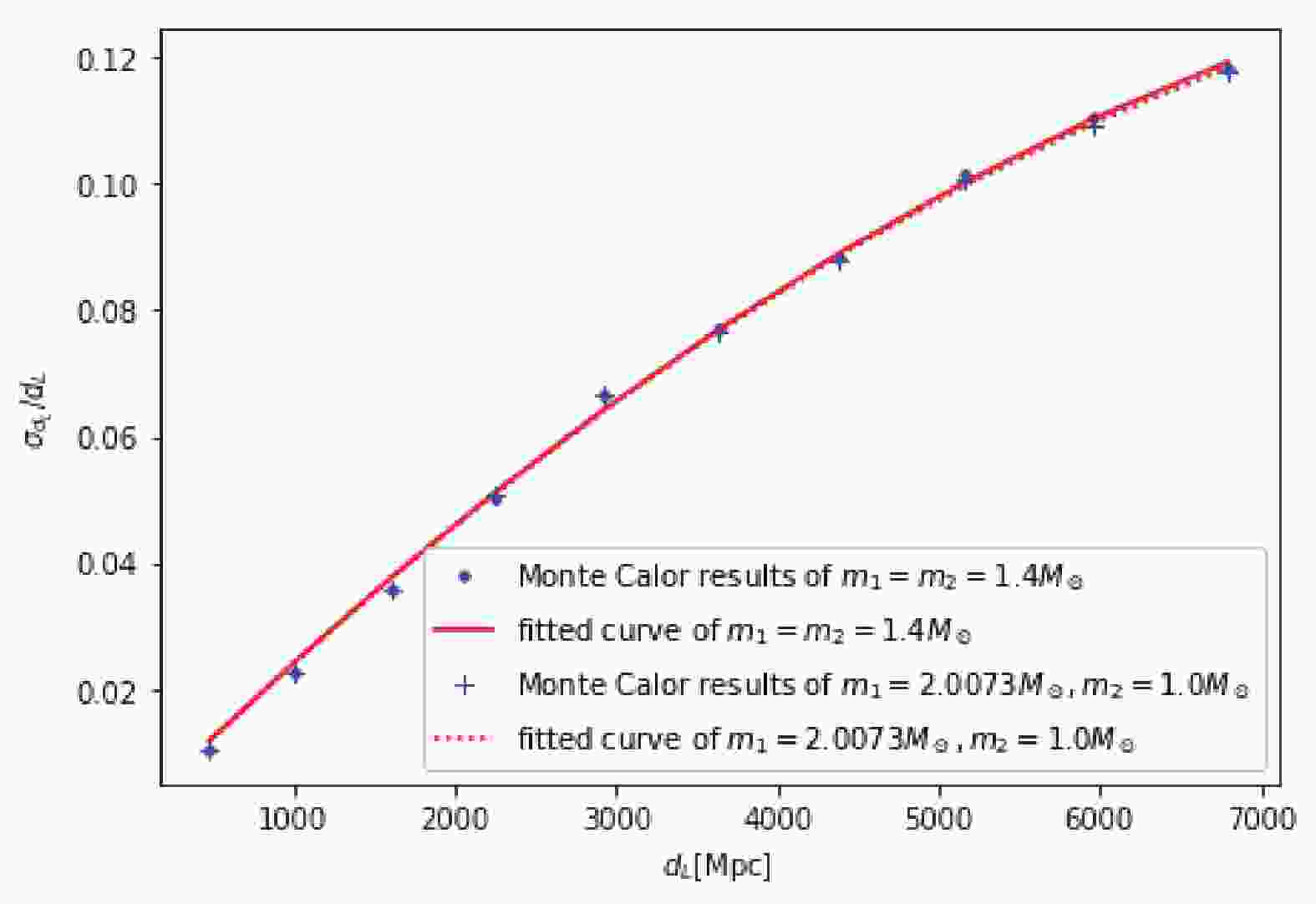
$ \sigma_{d_L}/d_L \sim d_L $ curve. We use a second-order polynomial to fit the curve and obtain$\begin{array}{*{20}{l}} {\displaystyle\frac{{{\sigma _{{d_L}}}}}{{{d_L}}}}&{ = - 1.15 \times {{10}^{ - 9}}d_L^2 + 2.53 \times {{10}^{ - 5}}{d_L}\;.} \end{array}$

(2) The
$ \sigma_{d_L}/d_L \sim d_L $ curve is ploted in Fig. 1. To investigate the effect of the deviation of neutron stars from the typical mass and mass ratio on the error bar of the luminosity distance, we reproduced the simulation for the case of a large mass ratio ($ m_1 = 2.0073M_{\odot}, m_2 = 1.0M_{\odot} $ . The chirp mass is almost equal to the case of$ m_1 = m_2 = 1.4M_{\odot} $ .). The corresponding curve is also plotted in Fig. 1. It can be seen that the two curves are almost the same. In the following calculation, we only use the curve for the case of equal masses.
Figure 1. (color online)
$\sigma_{d_L}/{d_L} $ as a function of redshift$d_L$ . The blue dots/pluses denote the results based on Monte Carlo sampling for the cases of equal mass and large mass ratio, respectively. The red solid curve denotes the fit (Eq. (2)) for the case of equal mass, and the red dashed line denotes the fit for the case of large mass ratio.In the simulations of the next section, the errors induced by weak lensing and peculiar velocity should also be considered. The total
$\sigma _{{d_L}}^{{\rm{total}}}$ can be written in this form:$\sigma _{{d_L}}^{{\rm{total}}} = \sqrt {{{({\sigma _{{d_L}}})}^2} + {{(\sigma _{{d_L}}^{{\rm{lens}}})}^2} + {{(\sigma _{{d_L}}^{{\rm{pv}}})}^2}} \;,$

(3) with
$\sigma _{{d_L}}^{{\rm{lens}}} = {d_L} \times 0.05z,$

(4) and
$\sigma _{{d_L}}^{{\rm{pv}}} = {d_L} \times \left| {1 - \frac{{{{(1 + z)}^2}}}{{H(z){d_L}(z)}}} \right|{\sigma _{{\rm{v}},{\rm{gal}}}}\;,$

(5) where
$ \sigma_{{d_L}}^{{\rm{lens}}}$ and$ \sigma_{{d_L}}^{{\rm{pv}}}$ are induced by the lensing magnification and the peculiar velocity of binaries [27, 28].$ \sigma _ { \rm { v } , \rm { gal } } $ is the one-dimensional velocity dispersion of the galaxy. It is often set to$ \sigma _ { \rm { v } , \rm { gal } } = 300\; \rm { km }\; \rm { s } ^ { - 1 } $ [38].$ H(z) $ and$ d_L(z) $ are the Hubble parameter and the luminosity distance given by the fiducial model. -
In this section, we first introduce the anisotropic model of cosmology. The anisotropic model possesses more parameters than
$ \Lambda $ CDM, one for anisotropic amplitude and two for anisotropic direction. We then use the relation$ \sigma_{{d_L}}^{{\rm{total}}}/d_L \sim d_L $ , obtained in the previous section, to study the uncertainties of the anisotropy parameters that could be observed by ET.The anisotropic model of cosmology can be described as a simple dipole model of the distance modulus. It has been discussed in Refs. [29, 39, 40]. The distance modulus in this model is of the form
$\mu = {\mu _{\Lambda {\rm{CDM}}}}(1 - d\cos \theta )\;,$

(6) where
${\mu _{\Lambda {\rm{CDM}}}} = 5\log \frac{{{d_L}}}{{{\rm{Mpc}}}} + 25\;,$

(7) and
$ \theta $ is the angle between the direction of space-time anisotropy and the direction of the event. The direction of space-time anisotropy can be parametrized as ($ l,b $ ) in the galactic coordinate system. d is the anisotropic amplitude and$ \mu_{\Lambda \rm{CDM}} $ is the distance modulus in the fiducial$ \Lambda $ CDM model. The fiducial parameters in this model are given by the result of Union2.1 [39], which are$ d = 0.0012, l = 310.6^\circ, $ $ b = -13^\circ $ .Next, we use the relation between
$ \sigma_{{d_L}}^{{\rm{total}}}$ and$ d_L $ to simulate the BNS merging events that could be observed by ET, and infer the relevant parameters ($ d, l, b $ ) in the anisotropic model of cosmology. We do our simulation as follows. For the case of 100 observed BNS merging events:1. The redshift of each event is referred to according to the event rate (
$ z\in(0,1) $ ) [27, 29]. After taking the time evolution of the burst rate into account, we can write the event rate in this form,$P(z) \propto \frac{{4\pi d_C^2(z)R(z)}}{{H(z)(1 + z)}},$

(8) where
$ d _ { C } = \int _ { 0 } ^ { z } 1 / H ( z ) {\rm d} z $ is the co-moving distance,$ H ( z ) $ is the Hubble parameter. Here we set$R(z) = 1 + 2z\;{\rm{for}}\; $ $z \leqslant {\rm{1}},R(z){\rm{ = }}({\rm{15 - 3}}z){\rm{/4}}\;{\rm{for}}\;{\rm{1}} < z < {\rm{5}}$ , and$ R ( z ) = 0 \;\rm { otherwise } $ . We multiply this event rate by the observed probability and get the new event rate. The observed probability is obtained from a simulation of 10000 events for every redshift point. We deem BNS events “GW detectable” when the network of ET has SNR$ >8 $ .2. We take the sky positions from a homogeneous distribution on the celestial sphere.
3. We use fiducial
$ \Lambda $ CDM to calculate the luminosity distances.4. The distance modulus is given by Eq. (7).
5. We use Eq. (6) to calculate the anisotropic distance modulus
${\mu _{{\rm{diople}}}}$ .6. By making use of the relation
$ \sigma_{{d_L}}^{{\rm{total}}}/d_L\sim d_L $ , we obtain the uncertainties of the luminosity distances.7. The uncertainty of the anisotropic distance modulus can be gotten from
${\sigma _\mu } = \frac{{5\sigma _{{d_L}}^{{\rm{total}}}}}{{\ln 10{d_L}}}\;.$

(9) 8. We re-sample every distance modulus from the Gaussion distribution
${\mu _{{\rm{sim}}}} \sim {\cal G}({\mu _{{\rm{diople}}}},{\sigma _\mu })$ 9. By making use of
$\{ ({\rm{ra}},{\rm{dec}}),{\mu _{{\rm{sim}}}},{\mu _{\Lambda {\rm{CDM}}}},{\sigma _\mu }\} $ , we constrain the anisotropic parameters.In this way, we get 100 sets of data. Each set contains five quantities:
$ \mu_{\Lambda\rm{CDM}}, l', b', \mu $ , and$ \sigma_{\mu} $ . The 100 sets of data are then used to fit the anisotropic model using the least-$ \chi^2 $ method, and the central values of ($ d,l, b $ ) and their uncertainties are obtained.We repeat the above procedures 800 times, and then calculate the average of uncertainties of (
$ d,l, b $ ). For 200, 300,..., and 1000 BNS merging events, the calculation method is the same as for 100 BNS merging events. Our results are presented in Fig. 2 to Fig. 5. In Fig. 2 and 3, the$ 1 \sigma $ confidence level is plotted.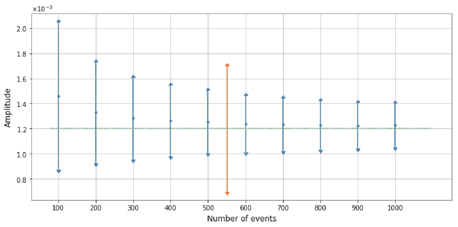
Figure 2. (color online) The average dipole amplitude and
$1 \sigma$ error as a function of the number of BNS merging events observed by ET. The dashed line is the fiducial dipole amplitude. The yellow line is the dipole amplitude of Union2.1.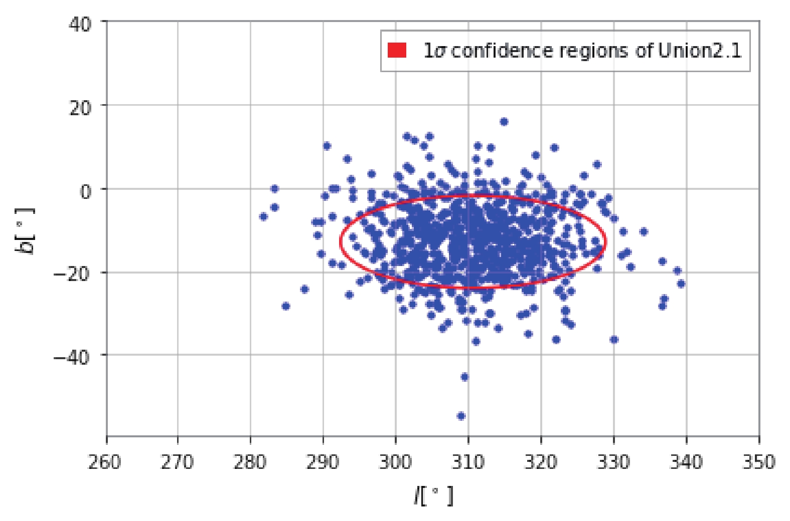
Figure 5. (color online) Distribution of preferred directions in 800 simulations, each with 1000 GW events observed by ET. The red error ellipse is the 1
$\sigma$ confidence region of Union2.1.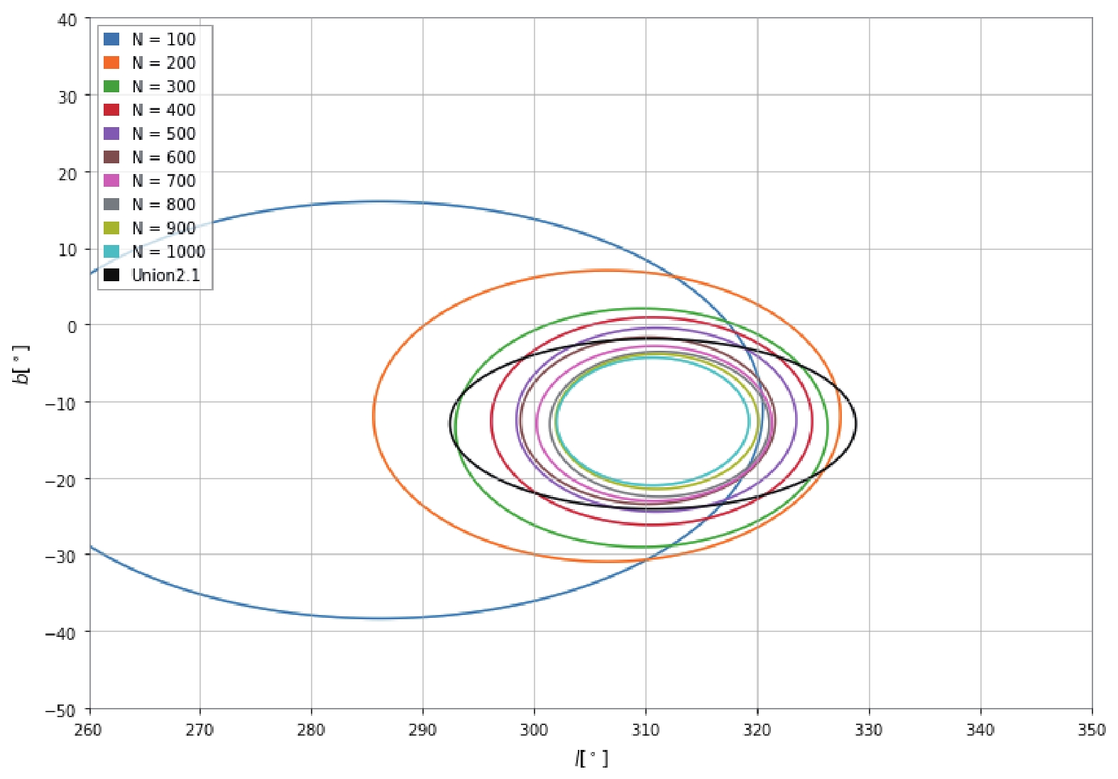
Figure 3. (color online) The average 1
$\sigma$ confidence region in the ($l,b$ ) plane for different number of GW events observed by ET. The 1$\sigma$ confidence region of Union2.1 is also plotted for comparison.Figure 2 shows the relation between the number of BNS merging events observed by ET and the inferred anisotropic amplitude. The uncertainties of the amplitudes are also plotted. The horizontal axis is the number of BNS merging events observed. The vertical axis is the inferred amplitude of the anisotropic parameter d and its uncertainty. It can be seen that when the number of BNS merging events observed increases, the uncertainty of the inferred amplitude becomes smaller. When 200 BNS merging events are observed by ET with the redshift in
$ (0,1) $ , it will be possible to determine the amplitude d with the accuracy of Union2.1 [39]. When the number of BNS merging events becomes larger, the incline of uncertainty reduction is gentle.Figure 3 shows the average 1
$ \sigma $ confidence region in the ($ l,b $ ) plane for different number of GW events observed by ET. The 1$ \sigma $ confidence region of Union2.1 is also plotted for comparison. The different color ellipses represent the anisotropic direction inferred for the different number of GW events. It can be seen that the inferred direction becomes more and more accurate as the number of observed BNS merging events increases. When the number of BNS merging events observed by ET reaches 400, it will be possible to determine the anisotropic direction with the accuracy of Union2.1 [39].Figure 4 shows the probability density map of the anisotropic amplitude inferred from 1000 simulated BNS merging events observed by ET. The distribution can be fitted by a Gaussian function centered at
$ 1.226\times10^{−3} $ , and with the standard deviation$ \sigma_{{d}} = 0.170\times10^{-3} $ . This implies that the fiducial dipole amplitude can be correctly reproduced with ~ 1000 GW events.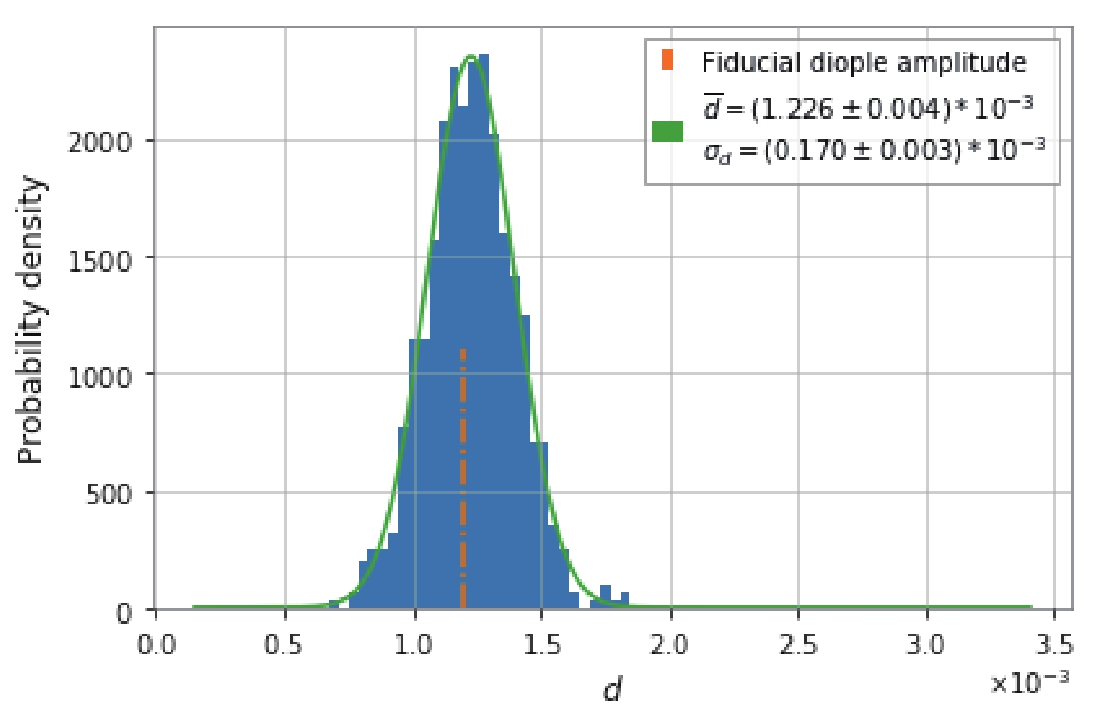
Figure 4. (color online) Probability density map of the anisotropic amplitude inferred from 1000 simulated BNS merging events observed by ET.
Figure 5 shows the distribution of preferred directions in 800 simulations, each with 1000 GW events observed by ET. The red error ellipse is the 1
$ \sigma $ confidence region of Union2.1. The percentage of points within the red circle in Fig. 5 is 73.5%. -
We used a new method to constrain the anisotropy of space-time by using GW. Unlike the Fisher matrix method, we simulated the process of extracting GW parameters from GW signals. By using the parameters of the future ET detector, we constrained the anisotropy of space-time. 200 BNS merging events with the redshift in (0,1) observed by ET guarantee that the accuracy of the constrained amplitude of the anisotropy of space-time would be the same as that of Union2.1.
In Ref. [28] , simulated data of GW events from BNS and black hole-neutron star binary (BHNS) were constructed for ET. It was found that with no less than 200 standard siren events, the cosmic isotropy can be ruled out at 3
$ \sigma $ C.L. if the dipole amplitude is larger than 0.06. This result is similar to ours. In Ref. [29], simulated data of GW events from binary black hole systems (BBH) were constructed for LIGO&Virgo. It was found that with no less than 400 GW events, the anisotropic amplitude can be constrained with an accuracy comparable to the Union2.1 complication of type-Ia supernovae. We used “BNS and ET” instead of “BBH and LIGO&Virgo”. Our result does not conflict with the result in Ref. [29].Cosmic Explorer (CE) is another planned 3rd generation GW detector, for which there is more hope that it will be constructed in the future. If there are 2 CE detectors, one in the U.S and one in Europe, the accuracy of
$ d_L $ will be worse than for ET [41]. Thus, if we use CE for the same simulation, the error bar of the inferred anisotropic amplitude will be larger than for ET. However, 3 CE detectors, one in the U.S., one in Europe and one in Australia, will give a better result.There are still some issues that need further discussions. Although the Planck 2018 result has been released [6], we have used the result obtained from Planck 2015 as it is very close to that from Planck 2018. In the future, we should not infer only the four parameters used above, but also try to include the angle of angular momentum of our line of sight,
$ \iota $ , by using BNS merging events. Studies have shown [37], that when$ - 20^\circ<\iota<20^\circ $ , one will also be able to see the electromagnetic signal.We are greatly appreciate Yong Zhou for useful discussions.
The prospects of using gravitational waves for constraining the anisotropy of the Universe
- Received Date: 2019-03-04
- Available Online: 2019-07-01
Abstract: The observation of GW150914 gave a new independent measurement of the luminosity distance of a gravitational wave event. In this paper, we constrain the anisotropy of the Universe by using gravitational wave events. We simulate hundreds of events of binary neutron star merger that may be observed by the Einstein Telescope. Full simulation of the production process of gravitational wave data is employed. We find that 200 binary neutron star merging events with the redshift in (0,1) observed by the Einstein Telescope may constrain the anisotropy with an accuracy comparable to that from the Union2.1 supernovae. This result shows that gravitational waves can be a powerful tool for investigating cosmological anisotropy.


 DownLoad: