


 Abstract
 HTML
HTML Reference
 Related
 PDF
PDF


-
Applying the method of integration by parts (IBP) [1], general scalar integrals can be reduced to a linear combination of scalar integrals. The calculation of scalar integrals represents an obstacle to the precise prediction of electroweak observables in the standard model. Whereas one-loop scalar integrals are computed [2,3], the calculations of the multi-loop scalar integrals are not advanced enough. A number of useful methods have been introduced in the literature to evaluate these scalar integrals in literature [4]. An analytical expression for the planar massless two-loop vertex diagrams is given in Ref. [5] using the Feynman parametrization method. The Mellin-Barnes (MB) method is occasionally used to compute some massless scalar integrals [6,7]. In the study of Ref. [8], the Mellin-Barnes representation was used to obtain expressions for some classes of single-loop massive Feynman integrals and vertex-type diagrams. The results are presented in the form of hypergeometric functions. Furthermore, multivariable hypergeometric functions are presented by explicit expressions for small and large momenta for two-loop self-energy diagrams [9]. However, the technique of multiple MB representations is highly cumbersome for a multi-loop diagram. For scalar integral, the authors of Refs. [10–24] derive a set of differential equations based on the IBP relationship. Another method is recommended to analyze the scalar integrals, which is referred to as "dimensional recurrence and analyticity'' [25–30]. The asymptotic expansion of momenta and masses can be employed to approach the scalar integral relying on kinematic invariants and masses [31]. A novel method [32,33] of computing Feynman integrals was proposed by constructing and solving a system of ordinary differential equations (ODEs).
The class of two-loop massive scalar self-energy diagrams with three propagators is studied in an arbitrary number of dimensions [34]. They can be described by generalized hypergeometric functions of several variables, namely Laricella functions. The results can be generalized to N loop massive scalar self-energy diagrams with N+1 propagators. However, only analytical results are obtained in the convergent regions. Their continuation from the convergent regions to the entire kinematic domain has not been completed.
For scalar integrals, the analytical expressions can be obtained through hypergeometric theory. According to the series representations of modified Bessel functions and some integrals from hypergeometric theory, in our previous work [35], we obtained the generalized hypergeometric functions of the one-loop B0 function, two-loop vacuum integral, the scalar integrals from the two-loop sunset and one-loop triangle diagrams. Moreover, we established the systems of linear homogeneous PDEs satisfied by the scalar integrals in the kinematic region. Furthermore, the C0 function has been calculated [36] under the guidance of MB representations. The continuation to the entire kinematic domain can be completed by applying the element method. The point specified here is that the system of homogeneous linear PDEs differs from that presented in the literature [10–20]. The detailed description is provided in Ref. [35]. The three-loop vacuum integrals with arbitrary masses are considered numerically in Refs. [37,38], which are the different methods compared with results of this study. The results of this study are consistent with the corresponding results of Ref. [37].
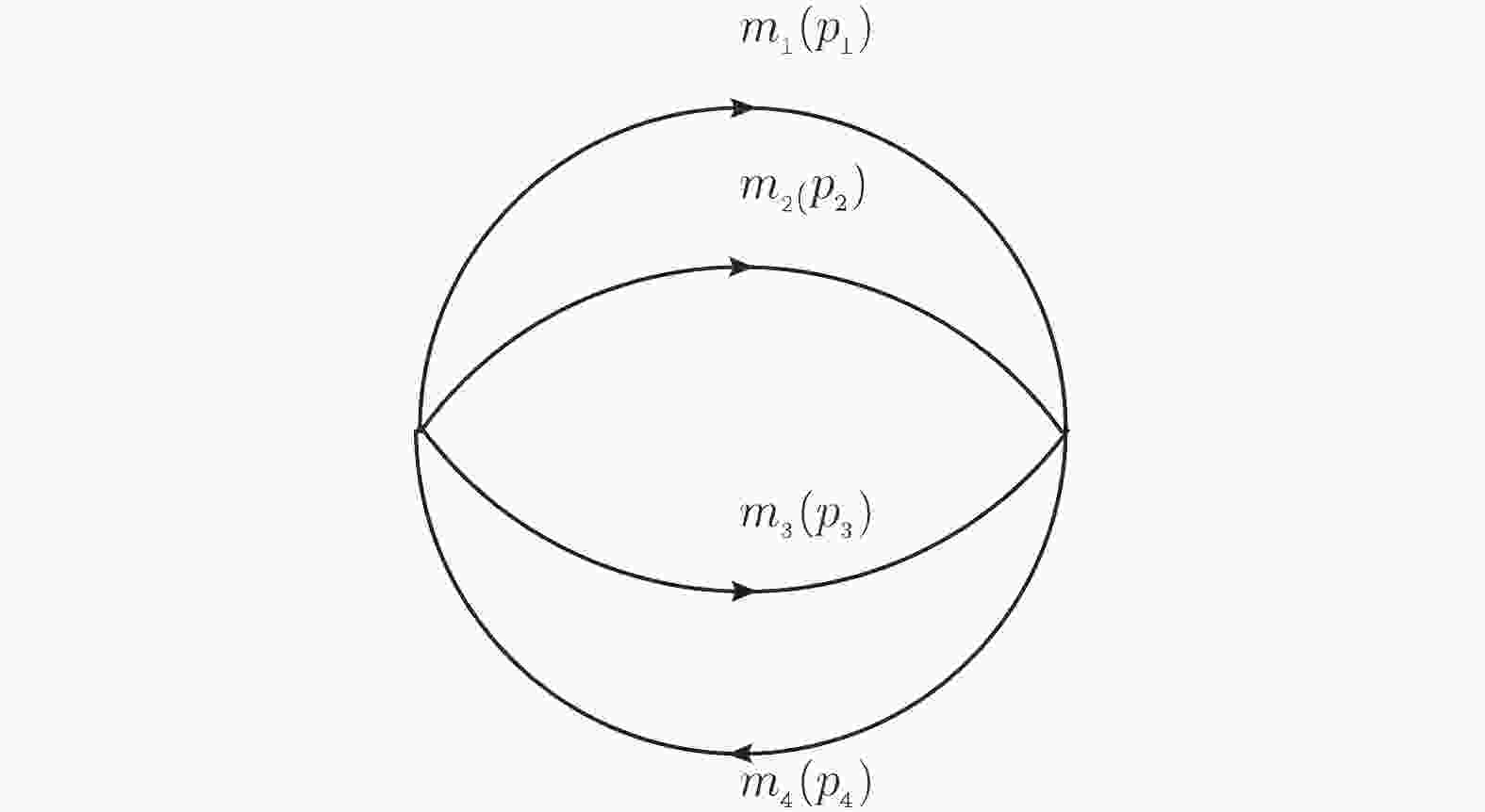
This study sets out to compute the scalar integral of the three-loop vacuum diagram Fig. 1. Our paper is organized as follows. In Section 2, the equivalence between the traditional Feynman parametrization and the hypergeometric theory for this scalar integral is verified. In Section 3, we obtain the generalized hypergeometric functions in terms of independent kinematic variables for the scalar integral, which are convergent in the connected region. Meanwhile, we note the systems of homogeneous linear partial differential equations (PDEs) satisfied by the corresponding generalized hypergeometric functions. According to the PDEs, the continuation from the convergent domain to the entire kinematic region can be completed by applying the finite element method. As a special case, the analytical results of the three-loop vacuum integral in the convergent region are presented in Section 4. Finally, our conclusions are summarized in Section 5.

Figure 1. Three-loop vacuum diagram,
$ m_{i} $ denotes the mass of the$ i $ -th particle and$ p_{j} $ depicts the corresponding momentum. -
The modified Bessel functions can be written in the following form [39-42]
$ \begin{split} {2(m^2)^{D/2-\alpha}\over(4\pi)^{D/2}\Gamma(\alpha)} k_{{D/2-\alpha}}(mx) =& \int{{\rm d}^Dq\over(2\pi)^D}{\exp[-i{ q}\cdot { x}]\over(q^2+m^2)^\alpha}\;,\\ {\Gamma(D/2-\alpha)\over(4\pi)^{D/2}\Gamma(\alpha)}\left({x\over2}\right)^{2\alpha-D} =& \int{{\rm d}^Dq\over(2\pi)^D}{\exp[-i{ q}\cdot { x}]\over(q^2)^\alpha}\;, \end{split} $

(1) where
$ { q} $ ,$ { x} $ are vectors in the D-dimension Euclid space, and$ m $ is the mass of the corresponding particle. After trivial cancellations of the numerator and denominator terms, the general analytic expression for the scalar integral of three-loop vacuum diagram Fig. 1 can be written in the form$ \begin{split} &U_{3}(m_{1}^2,m_{2}^2,m_{3}^2,m_{4}^2) = (\mu^2)^{6-3D/2}\int\prod\limits_{i = 1}^3{{\rm d}^Dp_{i}\over(2\pi)^D}\\&\quad \times{1\over(p_{1}^2-m_{1}^2)(p_{2}^2-m_{2}^2)(p_{3}^2-m_{3}^2)((p_{1}+p_{2}+p_{3})^2-m_{4}^2)}, \end{split} $

(2) where
$ D = 4-2\varepsilon $ is the number of dimensions in dimensional regularization and$ \mu $ denotes the renormalization energy scale. Applying the Wick rotation and Eq. (1), the three-loop$ U_{3} $ function is formulated as$\begin{split}& U_{3}(m_{1}^2,m_{2}^2,m_{3}^2,m_{4}^2) = {(-i)2^4(\mu^2)^{6-3D/2}\over\Gamma(D/2)(4\pi)^{3D/2}} \\&\quad \times \int_0^\infty {\rm d}x\prod\limits_{i = 1}^4(m_{i}^2)^{D/2-1} \left({x\over2}\right)^{D-1}k_{{D/2-1}}(m_{i}x)\;. \end{split}$

(3) The integral representation of the Bessel function can be applied to Eq. (3)
$ \begin{split}k_{\mu}(x) = {1\over2}\int_0^\infty t^{-\mu-1}\exp\left\{-t-{x^2\over4t}\right\}{\rm d}t\;, \quad \Re(x^2)> 0\;.\end{split} $

(4) Thus, the
$ U_{3} $ function is written as$ \begin{split} U_{3} =&{(-i)\left(\displaystyle\sum\limits_{i = 1}^4m_{i}^2\right)^{D/2-1}2^{1-D}(\mu^2)^{3D/2-6}\over(4\pi)^{3D/2}\Gamma(D/2)}\int_0^\infty {\rm d}t_{1}t_{1}^{-D/2} \int_0^\infty {\rm d}t_{2}t_{2}^{-D/2}\int_0^\infty {\rm d}t_{3}t_{3}^{-D/2}\int_0^\infty {\rm d}t_{4}t_{4}^{-D/2} \\ &\times \exp\{-t_{1}-t_{2}-t_{3}-t_{4}\}\int_0^\infty {\rm d}xx^{D-1} \exp\left\{\left(-{m_{1}^2\over4t_{1}}-{m_{2}^2\over4t_{2}}-{m_{3}^2\over4t_{3}}-{m_{4}^2\over4t_{4}}\right)x^2\right\} \end{split} $

$ \begin{split} =& {(-i)(\mu^2)^{6-3D/2}\over(4\pi)^{2D}}\int_0^\infty {\rm d}t_{1}t_{1}^{-D/2} \int_0^\infty {\rm d}t_{2}t_{2}^{-D/2}\int_0^\infty {\rm d}t_{3}t_{3}^{-D/2}\int_0^\infty {\rm d}t_{4}t_{4}^{-D/2} \\ &\times \exp\{-m_{1}^2t_{1}-m_{2}^2t_{2}-m_{3}^2t_{3}-m_{4}^2t_{4}\} \int {\rm d}^Dx\exp\left\{-{t_{1}t_{2}t_{3}+t_{1}t_{2}t_{4}+t_{1}t_{3}t_{4}+t_{2}t_{3}t_{4}\over4t_{1}t_{2}t_{3}t_{4}}x^2\right\} \\ = &{(-i)(\mu^2)^{6-3D/2}\over(4\pi)^{3D/2}}\int_0^\infty {\rm d} t_{1}t_{1}^{-D/2} \int_0^\infty {\rm d}t_{2}t_{2}^{-D/2}\int_0^\infty {\rm d}t_{3}t_{3}^{-D/2}\int_0^\infty {\rm d}t_{4}t_{4}^{-D/2} \\ &\times \exp\{-m_{1}^2t_{1}-m_{2}^2t_{2}-m_{3}^2t_{3}-m_{4}^2t_{4}\} \left({t_{1}t_{2}t_{3}t_{4}\over t_{1}t_{2}t_{3}+t_{1}t_{2}t_{4}+t_{1}t_{3}t_{4}+t_{2}t_{3}t_{4}}\right)^{D/2}\;. \end{split} $

(5) Performing the variable transformation
$ t_{1} = \varrho y_{1},\;t_{2} = \varrho y_{2},\;t_{3} = \varrho y_{3},\;t_{4} = \varrho (1-y_{1}-y_{2}-y_{3}),\; $

(6) the Jacobian of the transformation is
$ {\partial(t_{1},t_{2},t_{3},t_{4})\over\partial(y_{1},y_{2},y_{3},\varrho)} = \varrho^3\;, $

(7) finally, we have
$ \begin{split} U_{3} =& {(-i)(\mu^2)^{6-3D/2}\over(4\pi)^{3D/2}}\int_0^1{\rm d}y_{1}\int_0^1{\rm d}y_{2}\int_0^1{\rm d}y_{3}\times \int_0^\infty {\rm d}\varrho^{3-3D/2}\exp\{(-m_{1}^2y_{1}-m_{2}^2y_{2}-m_{3}^2y_{3}-m_{4}^2(1-y_{1}-y_{2}-y_{3}))\varrho\} \\&\times \Big({1\over y_{1}y_{2}y_{3}+y_{1}y_{2}(1-y_{1}-y_{2}-y_{3}) +y_{1}y_{3}(1-y_{1}-y_{2}-y_{3})+y_{2}y_{3}(1-y_{1}-y_{2}-y_{3})}\Big)^{D/2} \\ = &{(-i)\Gamma(4-3D/2)\over(4\pi)^{3D/2}(\mu^2)^{3D/2-6}}\int_0^1{\rm d}y_{1}\int_0^1{\rm d}y_{2}\int_0^1{\rm d}y_{3}\int_0^1{\rm d}y_{4}\delta(1-y_{1}-y_{2}-y_{3}-y_{4}) \\&\times {(m_{1}^2y_{1}+m_{2}^2y_{2}+m_{3}^2y_{3}+m_{4}^2y_{4})^{3D/2-4}\over(y_{1}y_{2}y_{3}+y_{1}y_{2}y_{4} +y_{1}y_{3}y_{4}+y_{2}y_{3}y_{4})^{D/2}}\;. \end{split} $

(8) The same result as Eq. (8) can be obtained while using the Feynman parametrization for the
$ U_{3} $ function. -
To obtain the triple hypergeometric series for the scalar integral from the three-loop vacuum diagram, the modified Bessel functions in power series an be written as
$ \begin{split} k_{{\mu}}(x) =& {1\over2}\sum\limits_{n = 0}^\infty{(-1)^n\over n!}\Big[ \Gamma(-\mu-n)\Big({x\over2}\Big)^{2n}+\Gamma(\mu-n)\Big({x\over2}\Big)^{2(n-\mu)}\Big] \\ =& {\Gamma(\mu)\Gamma(1-\mu)\over2}\sum\limits_{n = 0}^\infty{1\over n!}\Big[ -{1\over\Gamma(1+\mu+n)}\Big({x\over2}\Big)^{2n}\\&+{1\over\Gamma(1-\mu+n)}\Big({x\over2}\Big)^{2(n-\mu)}\Big]\;. \end{split} $

(9) The radial integral [39] can be presented as,
$ \int_0^\infty {\rm d}t \Big({t\over2}\Big)^{2\varrho-1}k_{\mu}(t) = {1\over2} \Gamma(\varrho)\Gamma(\varrho-\mu)\;. $

(10) According to the topology of Fig. 1, we can obtain a similar analytical expression, whichever
$ m_{i}(i = 1,2,3,4) $ is the maximum mass. Hence, we take the$ m_{4} $ maximum mass as an example to illustrate the calculation process. As$ m_{4}>\max(m_{1},m_{2},m_{3}) $ , inserting the expressions of$ k_{{D/2-1}}(m_{1}x) $ ,$ k_{{D/2-1}}(m_{2}x) $ ,$ k_{{D/2-1}}(m_{3}x) $ into Eq. (3) and subsequently applying Eq. (10), the$ U_{3} $ function is written as$ \begin{split} U_{3}(m_{1}^2,m_{2}^2,m_{3}^2,m_{4}^2) =& -{i({m_{4}^2})^{3D/2-4}(\mu^2)^{6-3D/2}\over\Gamma(D/2)(4\pi)^{3D/2}}\\&\times\Gamma^3\left({D\over2}-1\right)\Gamma^3\left(2-{D\over2}\right) \phi(x_{1},x_{2},x_{3})\;, \end{split} $

(11) with
$ x_{1} =\displaystyle\frac {m_{1}^2}{ m_{4}^2} $ ,$ x_{2} =\displaystyle\frac {m_{2}^2}{ m_{4}^2} $ , and$ x_{3} = \displaystyle\frac{m_{3}^2}{ m_{4}^2} $ . The function$ \phi(x_{1},x_{2},x_{3}) $ is defined as$ \begin{split} \phi(x_{1},x_{2},x_{3}) =& -{1\over\Gamma^2(D/2)}(x_{1}x_{2}x_{3})^{D/2-1} F_{C}^{(3)}\left(\left.\begin{array}{ccc}1,&D/2;&\;\\ D/2,&D/2,&D/2;\end{array}\right|x_{1},x_{2},x_{3}\right) \\&+{1\over\Gamma^2(D/2)}(x_{1}x_{2})^{D/2-1} F_{C}^{(3)}\left(\left.\begin{array}{ccc}1,&2-D/2;&\;\\ D/2,&D/2,&2-D/2;\end{array}\right|x_{1},x_{2},x_{3}\right)\end{split} $

(12) $ \begin{split} & +{1\over\Gamma^2(D/2)}(x_{1}x_{3})^{D/2-1} F_{C}^{(3)}\left(\left.\begin{array}{ccc}1,&2-D/2;&\;\\ D/2,&2-D/2,&D/2;\end{array}\right|x_{1},x_{2},x_{3}\right) \\ & +{1\over\Gamma^2(D/2)}(x_{2}x_{3})^{D/2-1} F_{C}^{(3)}\left(\left.\begin{array}{ccc}1,&2-D/2;&\;\\ 2-D/2,&D/2,&D/2;\end{array}\right|x_{1},x_{2},x_{3}\right) \\ & -{\Gamma(3-D)\over\Gamma(D/2)\Gamma(2-D/2)}(x_{1})^{D/2-1} F_{C}^{(3)}\left(\left.\begin{array}{ccc}2-D/2,&3-D;&\;\\ D/2,&2-D/2,&2-D/2;\end{array}\right|x_{1},x_{2},x_{3}\right) \\ & -{\Gamma(3-D)\over\Gamma(D/2)\Gamma(2-D/2)}(x_{2})^{D/2-1} F_{C}^{(3)}\left(\left.\begin{array}{ccc}2-D/2,&3-D;&\;\\ 2-D/2,&D/2,&2-D/2;\end{array}\right|x_{1},x_{2},x_{3}\right) \\ & -{\Gamma(3-D)\over\Gamma(D/2)\Gamma(2-D/2)}(x_{3})^{D/2-1} F_{C}^{(3)}\left(\left.\begin{array}{ccc}2-D/2,&3-D;&\;\\ 2-D/2,&2-D/2,&D/2;\end{array}\right|x_{1},x_{2},x_{3}\right) \\ & +{\Gamma(3-D)\Gamma(4-3D/2)\over\Gamma^3(2-D/2)} F_{C}^{(3)}\left(\left.\begin{array}{ccc}3-D,&4-3D/2;&\;\\ 2-D/2,&2-D/2,&2-D/2;\end{array}\right|x_{1},x_{2},x_{3}\right)\;. \end{split} $

(12) Here,
$ F_{C}^{(3)} $ is the Lauricella function of three independent variables$ \begin{split} &F_{C}^{(3)}\left(\left.\begin{array}{ccc}a,&b;&\;\\ c_{1},&c_{2},&c_{3};\end{array}\right|x_{1},x_{2},x_{3}\right) = \\&\quad \sum\limits_{n_{1} = 0}^\infty\sum\limits_{n_{2} = 0}^\infty \sum\limits_{n_{3} = 0}^\infty{(a)_{{n_{1}+n_{2}+n_{3}}}(b)_{{n_{1}+n_{2}+n_{3}}} \over n_{1}!n_{2}!n_{3}!(c_{1})_{{n_{1}}}(c_{2})_{{n_{2}}}(c_{3})_{{n_{3}}}} x_{1}^{n_{1}}x_{2}^{n_{2}}x_{3}^{n_{3}}\;,\end{split} $

(13) with the connected convergent region
$\sqrt{|x_{1}|}+\sqrt{|x_{2}|}+ $ $ \sqrt{|x_{3}|}\leqslant1 $ .For the case
$ m_{3}>\max(m_{1},m_{2},m_{4}) $ , one similarly derives$ \begin{split} U_{3}(m_{1}^2,m_{2}^2,m_{3}^2,m_{4}^2) = -{i({m_{3}^2})^{3D/2-4}(\mu^2)^{6-3D/2}\over\Gamma(D/2)(4\pi)^{3D/2}}\Gamma^3\left({D\over2}-1\right) \end{split} $

$ \begin{split}\times\Gamma^3\left(2-{D\over2}\right) \phi(y_{1},y_{2},y_{3})\;, \end{split} $

(14) with
$ y_{1} =\displaystyle\frac {m_{1}^2}{ m_{3}^2} = \displaystyle\frac{x_{1}}{ x_{3}} $ ,$ y_{2} = \displaystyle\frac{m_{2}^2}{ m_{3}^2} = \displaystyle\frac{x_{2}}{ x_{3}} $ , and$ y_{3} = \displaystyle\frac{m_{4}^2}{ m_{3}^2} = \displaystyle\frac{1}{ x_{3}} $ . We specify here that$ \phi(y_{1},y_{2},y_{3}) = (x_{3})^{4-3D/2}\phi(x_{1},x_{2},x_{3}) $ . For the case where$ m_{2}>\max(m_{1},m_{3},m_{4}) $ and$ m_{1}>\max(m_{2},m_{3},m_{4}) $ , we obtain similar results.Hence, when
$ D = 4-2\varepsilon $ , the analytic expression of the$ U_{3} $ function can be formulated as$ \begin{split} U_{3}(m_{1}^2,m_{2}^2,m_{3}^2,m_{4}^2) =& -{i\Gamma^3(1-\varepsilon)\Gamma^3(\varepsilon)\over\Gamma(2-\varepsilon)(4\pi)^4} \Big({m_{4}^2\over4\pi}\Big)^{2-3\varepsilon}\\&\times(\mu^2)^{3\varepsilon}\Phi_{U}(x_{1},x_{2},x_{3})\;, \end{split} $

(15) where
$ \begin{aligned} &\Phi_{U}(x_{1},x_{2},x_{3}) = \left\{\begin{array}{ll} \phi(x_{1},x_{2},x_{3})\;,&\sqrt{|x_{1}|}+\sqrt{|x_{2}|}+\sqrt{|x_{3}|}\leqslant1\;,\\ (x_{3})^{3D/2-4}\phi\left(\displaystyle\frac{x_{1}}{ x_{3}},\displaystyle\frac{x_{2}}{ x_{3}},\displaystyle\frac{1}{ x_{3}}\right)\;,&1+\sqrt{|x_{1}|}+\sqrt{|x_{2}|}\leqslant\sqrt{|x_{3}|}\;,\\ (x_{2})^{3D/2-4}\phi\left(\displaystyle\frac{x_{1}}{ x_{2}},\displaystyle\frac{x_{3}}{ x_{2}},\displaystyle\frac{1}{ x_{2}}\right),& 1+\sqrt{|x_{1}|}+\sqrt{|x_{3}|}\leqslant\sqrt{|x_{2}|}\;,\\ (x_{1})^{3D/2-4}\phi\left(\displaystyle\frac{x_{3}}{ x_{1}},\displaystyle\frac{x_{2}}{ x_{1}},\displaystyle\frac{1}{ x_{1}}\right),& 1+\sqrt{|x_{2}|}+\sqrt{|x_{3}|}\leqslant\sqrt{|x_{1}|}\;.\\ \end{array}\right. \end{aligned} $

(16) Here,
$ \Phi_{U}(x_{1},x_{2},x_{3}) $ satisfies the system of homogeneous linear PDEs [43, 44]$ \begin{split} &\left[\left(\sum_{i = 1}^3\hat{\vartheta}_{x_{i}}+3-D\right)\left(\sum_{i = 1}^3\hat{\vartheta}_{x_{i}}+4-{3D\over 2}\right) \right.\\&\quad\left.-{1\over x_{i}}\hat{\vartheta}_{x_{i}}\left(\hat{\vartheta}_{x_{i}}+1-{D\over2}\right)\right]\Phi_{U}(x_{1},x_{2},x_{3}) = 0\:, \end{split} $

(17) with
$ \hat{\vartheta}_{x_{i}} = x_{i}{\partial/\partial x_{i}}\;,i = 1,2,3. $ The
$ \Phi_{U} $ function under the restriction$ x_{2} = x_{3} = 0 $ is given as$ \begin{aligned} &\Phi_{U}(x_{1},0,0) = F(x_{1}) = \left\{\begin{array}{ll} \phi(x_{1},0,0)\;,&|x_{1}|\leqslant 1\\ (x_{1})^{3D/2-4}\phi\left(\displaystyle\frac{1}{ x_{1}},0,0\right)\;,&|x_{1}|\geqslant 1 \end{array}\right.\;. \end{aligned} $

(18) And one derives
$ \phi(x_{1},0,0) = (x_{1})^{3D/2-4}\phi\left(\displaystyle\frac{1}{ x_{1}},0,0\right) $ is thus derived. In the entire$ x_{1}- $ coordinate axis,$ F(x_{1}) $ depicts a continuous differentiable function.$ F(x_{1}) $ satisfies the first PDE with the condition$ x_{2} = x_{3} = 0 $ in Eq. (17). In a similar way, the analytical expressions for$ F(x_{2}), F(x_{3}) $ in the entire$ x_{2}, x_{3} $ -coordinate axis can be obtained. Taking the$ \Phi_{U}(x_{1},0,0) = $ $ F(x_{1})$ and$ \Phi_{U}(0,x_{2},0) = F(x_{2}) $ as boundary conditions, we can obtain the numerical solutions of$ \Phi_{U} $ on the entire$ x_{1}-x_{2} $ plane by the first two PDEs, when$ x_{3} = 0 $ . Employing a similar method, the continuation of$ \Phi_{U} $ to whole three-dimensional space can be completed through the system of PDEs in Eq. (17).We provide the Laurent series of the
$ U_{3}(m_{1}^2,m_{2}^2,m_{3}^2,m_{4}^2) $ function around space-time dimensions$ D = 4 $ to perform the numerical continuation of$ U_{3}(m_{1}^2,m_{2}^2,m_{3}^2,m_{4}^2) $ to entire kinematic regions,$ \begin{aligned} {U_{3}(m_{1}^2,m_{2}^2,m_{3}^2,m_{4}^2)} = (-i){(m_{4}^2)^2\over(4\pi)^6}\left({\mu^2\over m_{4}^2}\right)^{3\varepsilon}\times\left\{{\phi_{U}^{(-3)}(x_{1},x_{2},x_{3})\over\varepsilon^3}+ {\phi_{U}^{(-2)}(x_{1},x_{2},x_{3})\over\varepsilon^2} +{\phi_{U}^{(-1)}(x_{1},x_{2},x_{3})\over\varepsilon} +\sum\limits_{i = 0}^\infty\varepsilon^i\phi_{U}^{(i)}(x_{1},x_{2},x_{3})\right\}. \end{aligned} $

(19) The functions
$ \phi_{U}^{(-3)} $ ,$ \phi_{U}^{(-2)} $ ,$ \phi_{U}^{(-1)} $ ,$ \phi_{U}^{(0)} $ are expressed as follows:$ \phi_{U}^{(-3)}(x_{1},x_{2},x_{3}) = {\frac{1}{3}({x_{1}}+{x_{2}}+{x_{3}}+{x_{1}} {x_{2}}+{x_{1}} {x_{3}}+{x_{2}} {x_{3}})}\;, $

(20) $ \begin{split} \phi_{U}^{(-2)}(x_{1},x_{2},x_{3}) =& -\frac{1}{12}+\frac{4 }{3}({x_{1}}+{x_{2}}+{x_{3}}+{x_{1}}{x_{2}}+{x_{1}}{x_{3}}+{x_{2}}{x_{3}}) -\gamma_{E} ({x_{1}}+ {x_{2}}+ {x_{3}}+{x_{1}} {x_{2}}+ {x_{1}} {x_{3}}+ {x_{2}} {x_{3}})-\frac{1}{12}({x_{1}}^2+{x_{2}}^2+{x_{3}}^2)\\ &-\frac{1}{2} ({x_{1}} \ln x_{1}+ {x_{2}}\ln x_{2}+{x_{3}}\ln x_{3}+{x_{1}} {x_{2}} \ln x_{1}+ {x_{1}} {x_{3}} \ln x_{1}+{x_{1}} {x_{2}}\ln x_{2} +{x_{2}} {x_{3}}\ln x_{2}+{x_{1}} {x_{3}}\ln x_{3}+{x_{2}} {x_{3}}\ln x_{3})\;, \end{split} $

(21) $ \begin{split} \phi_{U}^{(-1)}(x_{1},x_{2},x_{3}) =& \left(-\frac{5}{8}+\frac{1}{4} {\gamma_{E}}\right) (1+{x_{1}}^2+{x_{2}}^2+{x_{3}}^2) +\left(\frac{10}{3}-4 {\gamma_{E}}+\frac{3}{2} {\gamma_{E}}^2 +\frac{1}{12}\pi ^2 \right)({x_{1}}+{x_{2}}+{x_{3}}+{x_{2}} {x_{3}}+{x_{1}} {x_{2}}+{x_{1}}{x_{3}})\\ & +\frac{3}{2} {\gamma_{E}} ( ({x_{2}}+{x_{3}}){x_{1}}\ln x_{1}+({x_{1}}+{x_{3}}){x_{2}}\ln x_{2}+({x_{1}}+{x_{2}}){x_{3}} \ln x_{3})+\left(\frac{3}{2}{\gamma_{E}}-2\right)( {x_{1}} \ln x_{1}+ {x_{2}} \ln x_{2}+ {x_{3}} \ln x_{3}) \\ &-2 ({x_{1}} {x_{2}}(\ln x_{1}+\ln x_{2})+ {x_{1}} {x_{3}}(\ln x_{1}+ \ln x_{3})+ {x_{2}} {x_{3}} (\ln x_{2}+ \ln x_{3}))+\frac{1}{4}({x_{1}}^2\ln x_{1}+ {x_{2}}^2 \ln x_{2}+ {x_{3}}^2 \ln x_{3}\\ &+ {x_{1}}\ln^2 x_{1}+{x_{2}} \ln^2 x_{2}+ {x_{3}} \ln^2 x_{3}+{x_{1}} {x_{2}}\ln^2 x_{1}+ {x_{1}} {x_{2}} \ln^2 x_{2}+ {x_{1}} {x_{3}}\ln^2 x_{1}+ {x_{1}} {x_{3}} \ln^2 x_{3}+ {x_{2}} {x_{3}} \ln^2 x_{2}\\ &+ {x_{2}} {x_{3}} \ln^2 x_{3})+{x_{1}} {x_{2}}\ln x_{1} \ln x_{2}+{x_{1}} {x_{3}}\ln x_{1} \ln x_{3}+{x_{2}} {x_{3}} \ln x_{2} \ln x_{3}\;, \end{split} $

(22) $ \begin{split} \phi_{U}^{(0)}(x_{1},x_{2},x_{3}) =& {\frac{1}{48} (-145+90 {\gamma_{E}}-18 {\gamma_{E}}^2-5 \pi ^2)}-\frac{1}{72} {x_{1}}\{3 (132-144 {\gamma_{E}}+54 {\gamma_{E}}^2+7 \pi ^2) \ln x_{1}+18 (-4+3 {\gamma_{E}})\ln^2 x_{1}+6\ln^3 x_{1}\\ &+2 (-218-216 {\gamma_{E}}^2+54 {\gamma_{E}}^3-12 \pi ^2+9 {\gamma_{E}} (40+\pi ^2)+11 \psi''(1)-5 \psi''(2))\}-\frac{1}{72} {x_{2}} \{3 (132-144 {\gamma_{E}}+54 {\gamma_{E}}^2\\ &+7 \pi ^2) \ln x_{2}+18 (-4+3 {\gamma_{E}})\ln^2 x_{2}+6 \ln^3 x_{2}+2 (-218-216 {\gamma_{E}}^2+54 {\gamma_{E}}^3-12 \pi ^2+9 {\gamma_{E}} (40+\pi ^2)+11 \psi''(1)\\ &-5 \psi''(2))\}-\frac{1}{72} {x_{3}} \{3 (132-144 {\gamma_{E}}+54 {\gamma_{E}}^2+7 \pi ^2) \ln x_{3}+18 (-4+3 {\gamma_{E}})\ln^2 x_{3}+6 \ln^3 x_{3}+2 (-218-216 {\gamma_{E}}^2\\ &+54 {\gamma_{E}}^3-12 \pi ^2+9 {\gamma_{E}} (40+\pi ^2)+11 \psi''(1)-5 \psi''(2))\}-\frac{1}{48} {x_{1}}^2 (43-90 {\gamma_{E}}+18 {\gamma_{E}}^2-3 \pi ^2+6 (-5+6 {\gamma_{E}}) \ln x_{1}\\ &+6\ln^2 x_{1}){-\frac{1}{48} {x_{2}}^2 (43-90 {\gamma_{E}}+18 {\gamma_{E}}^2-3 \pi ^2+6 (-5+6 {\gamma_{E}}) \ln x_{2}+6 \ln^2 x_{2})}-\frac{1}{48} {x_{3}}^2 (43-90 {\gamma_{E}}+18 {\gamma_{E}}^2-3 \pi ^2\\ &+6 (-5+6 {\gamma_{E}}) \ln x_{3}+6 \ln^2 x_{3})-\frac{1}{72} {x_{1}} {x_{2}} \{-432 {\gamma_{E}}^2+108 {\gamma_{E}}^3+18 {\gamma_{E}} (40+\pi ^2)+6 \ln^3 x_{1}+ 3 (108-144 {\gamma_{E}}+54 {\gamma_{E}}^2\\ &-\pi ^2) \ln x_{2}+18 (-4+3 {\gamma_{E}}) \ln^2 x_{2}+6 \ln^3 x_{2}+18 \ln^2 x_{1} (-4+3 {\gamma_{E}}+2 \ln x_{2})+3 \ln x_{1} (108-144 {\gamma_{E}}+54 {\gamma_{E}}^2-\pi ^2\\ &+72 (-1+{\gamma_{E}}) \ln x_{2}+12 \ln^2 x_{2})-4 (106+11 \psi''(1)+4\psi''(2))\}-\frac{1}{72} {x_{1}} {x_{3}}\{-432 {\gamma_{E}}^2+108 {\gamma_{E}}^3+18 {\gamma_{E}} (40+\pi ^2)\\ &+6 \ln^3 x_{1}+ 3 (108-144 {\gamma_{E}}+54 {\gamma_{E}}^2-\pi ^2) \ln x_{3}+18 (-4+3 {\gamma_{E}}) \ln^2 x_{3}+6 \ln^3 x_{3}+18 \ln^2 x_{1} (-4+3 {\gamma_{E}}+2 \ln x_{3})\\ &+3 \ln x_{1} (108-144 {\gamma_{E}}+54 {\gamma_{E}}^2-\pi ^2+72 (-1+{\gamma_{E}}) \ln x_{3}+12 \ln^2 x_{3})-4(106+11\psi''(1)+4\psi''(2))\}\\ &-\frac{1}{72} {x_{2}} {x_{3}}\{-432 {\gamma_{E}}^2+108 {\gamma_{E}}^3+18 {\gamma_{E}} (40+\pi ^2)+6 \ln^3 x_{2}+ 3 (108-144 {\gamma_{E}}+54 {\gamma_{E}}^2-\pi ^2) \ln x_{3}\\ &+18 (-4+3 {\gamma_{E}}) \ln^2 x_{3}+6 \ln^3 x_{3}+18 \ln^2 x_{2} (-4+3 {\gamma_{E}}+2 \ln x_{3})+3 \ln x_{2} (108-144 {\gamma_{E}}+54 {\gamma_{E}}^2\\ &-\pi ^2+72 (-1+{\gamma_{E}}) \ln x_{3}+12 \ln^2 x_{3})-4 (106+11 \psi''(1)+4 \psi''(2))\}+\phi_0^{(0)}(x_{1},x_{2},x_{3}). \end{split} $

(23) The expression of function
$ \phi_0^{(0)}(x_{1},x_{2},x_{3}) $ is given in Appendix A. The results of Eq. (20), Eq. (21), and Eq. (22) are consistent with the result of Ref. [37]. Furthermore, the expression of Eq. (23) is superior to the result of Ref. [37]. The systems of linear PDEs in Appendix B are derived, and they are satisfied by the functions$ \phi_{U}^{(-3)} $ ,$ \phi_{U}^{(-2)} $ , and$ \phi_{U}^{(i)}(i = -1,\;0,\;1,\;2,\;\cdots) $ .Through the systems of PDEs in Appendix B, the continuation of the numerical solution of the triple hypergeometric series can be made to the entire kinematic domain. The derived
$ \phi_{U}^{(-3)} \!=\!\left\{ \displaystyle\frac{1}{3}({x_{1}}\!+\!{x_{2}}\!+\!{x_{3}}\!+\!{x_{1}} {x_{2}}\!+\!{x_{1}} {x_{3}}\!+\!{x_{2}} {x_{3}})\right\} $ satisfies Eq. (B1) explicitly. After obtaining the solutions$ \phi_{U}^{(n-2)} $ and$ \phi_{U}^{(n-1)} $ , one writes$ F = x_{1}^{-1/2}x_{2}^{-1/2}x_{3}^{-1/2}\phi_{U}^{(n)} $ satisfies the system of linear PDEs as follows:$ \begin{split} 2x_{1}{\partial^2F\over\partial x_{1}^2}&-x_{2}{\partial^2F\over\partial x_{2}^2} -x_{3}{\partial^2F\over\partial x_{3}^2} +2{\partial F\over\partial x_{1}}-{\partial F\over\partial x_{2}} -{\partial F\over\partial x_{3}} \\&+\left(-{1\over 2x_{1}}+{1\over4x_{2}}+{1\over4x_{3}}\right)F -x_{1}^{-1/2}x_{2}^{-1/2}x_{3}^{-1/2}\\&\times(2g_{1}-g_{2}-g_{3}) = 0 \;,\\ x_{2}{\partial^2F\over\partial x_{2}^2} &-x_{3}{\partial^2F\over\partial x_{3}^2} +{\partial F\over\partial x_{2}}-{\partial F\over\partial x_{3}} +\left(-{1\over4x_{2}}+{1\over4x_{3}}\right)F \\&-x_{1}^{-1/2}x_{2}^{-1/2}x_{3}^{-1/2}(g_{2}-g_{3}) = 0 \;,\\ x_{1}^2{\partial^2F\over\partial x_{1}^2} &+x_{2}^2{\partial^2F\over\partial x_{2}^2} +x_{3}(x_{3}-1){\partial^2F\over\partial x_{3}^2} +2x_{1}x_{2}{\partial^2F\over\partial x_{1}\partial x_{2}}\\&+2x_{1}x_{3}{\partial^2F\over\partial x_{1}\partial x_{3}} +2x_{2}x_{3}{\partial^2F\over\partial x_{2}\partial x_{3}} +x_{1}{\partial F\over\partial x_{1}} \\& +x_{2}{\partial F\over\partial x_{2}}+(x_{3}-1){\partial F\over\partial x_{3}}+\left({1\over 4x_{3}}-{1\over 4}\right)F \\& -x_{1}^{-1/2}x_{2}^{-1/2} x_{3}^{-1/2}g_{3} = 0\;, \end{split} $

(24) and
$ \begin{split} g_{1}(x_{1},x_{2},x_{3}) =& -(1-5x_{1}){\partial\phi_{U}^{(n-1)}\over\partial x_{1}} +5x_{2}{\partial\phi_{U}^{(n-1)}\over\partial x_{2}} \\&+5x_{3}{\partial\phi_{U}^{(n-1)}\over\partial x_{3}} -7\phi_{U}^{(n-1)}+6\phi_{U}^{(n-2)} \;,\\ g_{2}(x_{1},x_{2},x_{3}) =& 5x_{1}{\partial\phi_{U}^{(n-1)}\over\partial x_{1}} -(1-5x_{2}){\partial\phi_{U}^{(n-1)}\over\partial x_{2}} \\&+5x_{3}{\partial\phi_{U}^{(n-1)}\over\partial x_{3}} -7\phi_{U}^{(n-1)}+6\phi_{U}^{(n-2)} \;,\\ g_{3}(x_{1},x_{2},x_{3}) =& 5x_{1}{\partial\phi_{U}^{(n-1)}\over\partial x_{1}} +5x_{2}{\partial\phi_{U}^{(n-1)}\over\partial x_{2}} \\&-(1-5x_{3}){\partial\phi_{U}^{(n-1)}\over\partial x_{3}} -7\phi_{U}^{(n-1)}+6\phi_{U}^{(n-2)}\;. \end{split} $

(25) The second and third PDEs in Eq. (24) are recognized as the constraints of the function
$ F(x_{1},x_{2},x_{3}) $ . The system of PDEs in Eq. (24) is recognized as the modified function based on the constrained variational principle [45],$\begin{split} {\Pi _U^*(F)} =&{ {\Pi _U}(F)} + \int\limits_\Omega {{\chi _{23}}} \left\{ {x_2}\frac{{{\partial ^2}F}}{{\partial x_2^2}} - {x_3}\frac{{{\partial ^2}F}}{{\partial x_3^2}} + \frac{{\partial F}}{{\partial {x_2}}} - \frac{{\partial F}}{{\partial {x_3}}} \right.\\&\left.+ \left( - \frac{1}{{4{x_2}}} + \frac{1}{{4{x_3}}}\right)F - x_1^{ - 1/2}x_2^{ - 1/2}x_3^{ - 1/2}({g_2} - {g_3})\right\} \\ &\times {\rm d}{x_1}{\rm d}{x_2}{\rm d}{x_3} + \int\limits_\Omega {\chi _{123}} \Bigg\{ x_1^2\frac{{{\partial ^2}F}}{{\partial x_1^2}} + x_2^2\frac{{{\partial ^2}F}}{{\partial x_2^2}} \\&+ {x_3}({x_3} - 1)\frac{{{\partial ^2}F}}{{\partial x_3^2}} + 2{x_1}{x_2}\frac{{{\partial ^2}F}}{{\partial {x_1}\partial {x_2}}} + 2{x_1}{x_3}\frac{{{\partial ^2}F}}{{\partial {x_1}\partial {x_3}}} \\&+ 2{x_2}{x_3}\frac{{{\partial ^2}F}}{{\partial {x_2}\partial {x_3}}} + {x_1}\frac{{\partial F}}{{\partial {x_1}}} + {x_2}\frac{{\partial F}}{{\partial {x_2}}} + ({x_3} - 1)\frac{{\partial F}}{{\partial {x_3}}}\\ &+ \left(\frac{1}{{4{x_3}}} - \frac{1}{4}\right)F - x_1^{ - 1/2}x_2^{ - 1/2}x_3^{ - 1/2}{g_3}\Bigg\} {\rm d}{x_1}{\rm d}{x_2}{\rm d}{x_3}\:, \end{split}$

(26) where
$ \chi_{{23}}(x_{2},x_{3}),\;\chi_{{123}}(x_{1},x_{2},x_{3}) $ are Lagrange multipliers.$ \Omega $ represents the kinematic domain of the numerical solution, and$ \Pi_{U}(F) $ is the function of the first PDE in Eq. (24):$ \begin{split} \Pi_{U}(F) =& \int\limits_{\Omega}\Bigg\{ x_{1}\left({\partial F\over\partial x_{1}}\right)^2 -{x_{2}\over2}\left({\partial F\over\partial x_{2}}\right)^2 -{x_{3}\over2}\left({\partial F\over\partial x_{3}}\right)^2 \\&-\left[-{1\over 4x_{1}}+{1\over8x_{2}} +{1\over8x_{3}}\right]F^2 +x_{1}^{-1/2}x_{2}^{-1/2}x_{3}^{-1/2} \\ &\times\Big(2g_{1}-g_{2}-g_{3}\Big)F\Bigg\}{\rm d}x_{1}{\rm d}x_{2}{\rm d}x_{3}\;. \end{split} $

(27) Firstly, the corresponding function expression of one coordinate axis is taken as the boundary condition, such that the numerical solution of the planes can be obtained. Subsequently, the entire kinematic region can obtain the numerical solution by the finite element method [45].
The continuation of function
$ U_{3} $ can be calculated differently. Hence, the method of the Mellin-Barnes representation [46,47] can be used to evaluate the scalar integrals in this case:$ \begin{aligned} {1\over (k^2-M^2)^v} = {1\over \Gamma(v)}{1\over 2\pi i}\int_{-i\infty}^{i\infty}{\rm d}s{(-M^2)^s\over (k^2)^{v+s}}\Gamma(-s)\Gamma(v+s)\;. \end{aligned} $

(28) Applying Eq. (28) to Eq. (2), we obtain
$ \begin{split} U_{3}(m_{1}^2,m_{2}^2,m_{3}^2,m_{4}^2) =& {(-i)(m_4^2)^{3D/2-4}(\mu^2)^{6-3D/2}\over(4\pi)^{3D/2}\Gamma(D/2)} {1\over (2\pi i)^3}\\&\times\int_{-i\infty}^{i\infty}\int_{-i\infty}^{i\infty}\int_{-i\infty}^{i\infty}{\rm d}{s_{1}}{\rm d}{s_{2}}{\rm d}{s_{3}} x_{1}^{s_{1}}x_{2}^{s_{2}}x_{3}^{s_{3}}\\ &\times\Gamma(-s_{1})\Gamma(-s_{2})\Gamma(-s_{3})\Gamma(D/2-1-s_{1})\\&\times\Gamma(D/2-1-s_{2})\Gamma(D/2-1-s_{3})\\ &\times\Gamma(4-3D/2+s_{1}+s_{2}+s_{3})\\&\times\Gamma(3-D+s_{1}+s_{2}+s_{3})\;. \end{split} $

(29) Using the result of [43], Eq. (29) is written as
$ \begin{split} U_{3}(m_{1}^2,m_{2}^2,m_{3}^2,m_{4}^2) =& {(-i)(m_4^2)^{3D/2-4}(\mu^2)^{6-3D/2}\over(4\pi)^{3D/2}\Gamma(D/2)} {1\over (2\pi i)^3}\int_{-i\infty}^{i\infty}\int_{-i\infty}^{i\infty}\int_{-i\infty}^{i\infty}{\rm d}{s_{1}}{\rm d}{s_{2}}{\rm d}{s_{3}} (-1)^{s_{1}}(1-x_{1})^{s_{1}}x_{2}^{s_{2}}x_{3}^{s_{3}}\Gamma(-s_{1})\Gamma(-s_{2})\\ &\times\Gamma(-s_{3})\Gamma(D/2-1-s_{2})\Gamma(D/2-1-s_{3})\Gamma(4-3D/2+s_{2}+s_{3})\Gamma(3-D+s_{2}+s_{3})\\ &\times{\Gamma(4-3D/2+s_{1}+s_{2}+s_{3})\Gamma(3-D+s_{1}+s_{2}+s_{3})\over\Gamma(6-2D+s_{1}+2s_{2}+2s_{3})}\;. \end{split} $

(30) We close the integration contour in Eq. (30) to the right and obtain
$ \begin{split} U_{3}(m_{1}^2,m_{2}^2,m_{3}^2,m_{4}^2) =& {(-i)(m_4^2)^{3D/2-4}(\mu^2)^{6-3D/2}\over(4\pi)^{3D/2}\Gamma(D/2)}\Bigg\{{\Gamma^2(D/2-1)\Gamma^2(3-D)\Gamma(4-3D/2)\over\Gamma^3(2-D/2)\Gamma(6-2D)}\\ &\times\;\Phi_{1;1}^{2;2}\left(\left.\begin{array}{cccc}3-D,&4-3D/2,&3-D,&2-D/2;\\ 6-2D;&2-D/2,&2-D/2;\end{array}\right|{1-x_{1}},x_{2},x_{3}\right)+{\Gamma(D/2-1)\Gamma(1-D/2)\Gamma(3-D)\over\Gamma^2(D/2)\Gamma(4-D)}\\ &\times\;x_{2}^{D/2-1}\Phi_{1;1}^{2;2}\left(\left.\begin{array}{cccc}2-D/2,&3-D,&2-D/2,&1;\\ 4-D;&D/2,&2-D/2;\end{array}\right|{1-x_{1}},x_{2},x_{3}\right)+{\Gamma(D/2-1)\Gamma(1-D/2)\Gamma(3-D)\over\Gamma^2(D/2)\Gamma(4-D)}\\ &\times\;x_{3}^{D/2-1}\Phi_{1;1}^{2;2}\left(\left.\begin{array}{cccc}2-D/2,&3-D,&2-D/2,&1;\\ 4-D;&D/2,&2-D/2;\end{array}\right|{1-x_{1}},x_{2},x_{3}\right)+{\Gamma(2-D/2)\Gamma^2(1-D/2)\over\Gamma^3(D/2)}\\ &\times\;(x_{2} x_{3})^{D/2-1}\Phi_{1;1}^{2;2}\left(\left.\begin{array}{cccc}1,&D/2,&1,&2-D/2;\\ 2;&D/2,&D/2;\end{array}\right|{1-x_{1}},x_{2},x_{3}\right) \Bigg\}\;. \end{split} $

(31) Here,
$ \Phi_{1;1}^{2;2} $ can be expressed as$ \begin{aligned} \Phi_{1;1}^{2;2}\left(\left.\begin{array}{cccc}a_{1},&a_{2};&b_{1},&b_{2}\;\\ c_{1};&d_{1},&d_{2};\end{array}\right|x_{1},x_{2},x_{3}\right) = \sum\limits_{n_{1} = 0}^\infty\sum\limits_{n_{2} = 0}^\infty \sum\limits_{n_{3} = 0}^\infty{(a_{1})_{{n_{1}+n_{2}+n_{3}}}(a_{2})_{{n_{1}+n_{2}+n_{3}}} (b_{1})_{{n_{2}+n_{3}}}(a_{2})_{{n_{2}+n_{3}}} \over n_{1}!n_{2}!n_{3}!(c_{1})_{{n_{1}+2n_{2}+2n_{3}}}(d_{1})_{{n_{2}}}(d_{2})_{{n_{3}}}} x_{1}^{n_{1}}x_{2}^{n_{2}}x_{3}^{n_{3}}\;, \end{aligned} $

(32) with the connected convergent region
$ \sqrt{|x_{1}|}+\sqrt{|x_{2}|}+$ $ \sqrt{|x_{3}|}\leqslant 1 $ . The continuation of Eq. (11) from$ \sqrt{|x_{1}|}+\sqrt{|x_{2}|}+$ $ \sqrt{|x_{3}|}\leqslant 1 $ to$ \sqrt{|1-x_{1}|}+\sqrt{|x_{2}|}+\sqrt{|x_{3}|}\leqslant 1 $ can be completed by this step. -
In this section, we deal with a situations different from the one described above.
-
When a variable is equal to one in Eq. (16), the analytical expression of the
$ U_{3} $ function can be simplified. We adopt the following formulae [48]$ \begin{aligned} &\;_{2}F_{1}\left(\left.\begin{array}{cc}a,&b\\ &c\end{array}\right| 1\right) = {\Gamma(c)\Gamma(c-a-b)\over\Gamma(c-a)\Gamma(c-b)}\;, \end{aligned} $

(33) in the case where
$ Rl(c-a-b)>0) $ . With the help of Eq. (33), the$ F_{C}^{(3)} $ function can turn to be$ \begin{aligned} F_{C}^{(3)}\left(\left.\begin{array}{ccc}a,&b;&\;\\ c_{1},&c_{2},&c_{3};\end{array}\right|1,x_{2},x_{3}\right) = {\Gamma({c_1})\Gamma({c_1}-a-b) \over\Gamma({c_1}-a)\Gamma({c_1}-b)} \;F_{2;1}^{4;0}\left(\left.\begin{array}{cccc}a,&b,&{1+a-c_{1}},&{1+b-c_{1}};\\ \displaystyle\frac{1+a+b-c_{1}}{2},&\displaystyle\frac{2+a+b-c_{1}}{2};&c_{2},&c_{3};\end{array}\right|{x_{2}\over4},{x_{3}\over4}\right) \end{aligned} $

(34) and
$ F_{2;1}^{4;0} $ is the Kamp$ \acute{e} $ de F$ \acute{e} $ riet function [49]$ \begin{aligned} F_{C;D}^{A;B}\left(\left.\begin{array}{ccccc}&a_{1},&\cdots, &a_{A};\\b_{1},&b_{1}^{'},&\cdots,&b_{B},&b_{B}^{'};\\ &c_{1},&\cdots, &c_{C};\\d_{1},&d_{1}^{'},&\cdots,&d_{D},&d_{D}^{'}; \end{array}\right|x,y\right) = \sum_{m = 0}^\infty\sum_{n = 0}^\infty{}{\prod_{j = 1}^{A}(a_j)_{m+n}\prod_{j = 1}^{B}(b_j)_{m}(b_j)^{'}_{n}\over \prod_{j = 1}^{C}(c_j)_{m+n}\prod_{j = 1}^{D}(d_j)_{m}(d_j)^{'}_{n} m!n!}x^my^n\;. \end{aligned} $

(35) Using Eq. (34) and performing some simplification, we obtain the results
$ \begin{aligned} &U_{3}(m^2,m^2,m_{3}^2,m_{4}^2) = {(-i)(m^2)^{3D/2-4}(\mu^2)^{6-3D/2}\over(4\pi)^{3D/2}\Gamma(D/2)}\omega\left({x\over4},{y\over4}\right)\;, \end{aligned} $

(36) and
$ \omega(x,y) $ is given by$ \begin{split} \omega\left({x\over4},{y\over4}\right) =& {\Gamma(4-3D/2)\Gamma^2(3-D)\Gamma(2-D/2)\Gamma^2(D/2-1)\over \Gamma(6-2D)}\times\;F_{1;1}^{3;0}\left(\left.\begin{array}{ccc}4-3D/2,&3-D,&2-D/2;\\ 7/2-D;&2-D/2,&2-D/2;\end{array}\right|{{x\over4},{y\over4}}\right)\\ & +{\Gamma(3-D)\Gamma^2(2-D/2)\Gamma(D/2-1)\Gamma(1-D/2)\over \Gamma(4-D)}(x)^{D/2-1}\times\;F_{1;1}^{3;0}\left(\left.\begin{array}{ccc}3-D,&2-D/2,&1;\\ 5/2-D/2;&D/2,&2-D/2;\end{array}\right|{{x\over4},{y\over4}}\right)\\ &+{\Gamma(3-D)\Gamma^2(2-D/2)\Gamma(D/2-1)\Gamma(1-D/2)\over \Gamma(4-D)}(y)^{D/2-1}\times\;F_{1;1}^{3;0}\left(\left.\begin{array}{ccc}3-D,&2-D/2,&1;\\ 5/2-D/2;&2-D/2,&D/2;\end{array}\right|{{x\over4},{y\over4}}\right)\\ &+{\Gamma(D/2)\Gamma(2-D/2)\Gamma^2(1-D/2)\over \Gamma(2)}(xy)^{D/2-1}\times\;F_{1;1}^{3;0}\left(\left.\begin{array}{ccc}2-D/2,&1,&D/2;\\ 3/2;&D/2,&D/2;\end{array}\right|{{x\over4},{y\over4}}\right)\;, \end{split} $

(37) with
$ x = m_{3}^2/ m^2,\;y = m_{4}^2/ m^2 $ . The$ F_{1;1}^{3;0} $ convergent region is$ \sqrt{|{\displaystyle\frac{x}{4}}|}+\sqrt{|{\displaystyle\frac{y}{4}}|}\leqslant 1 $ . If we use the method of the Mellin-Barnes representation on Eq. (2), we can obtain the same result as Eq. (37). Moreover, the function$ \omega(x,y) = \omega\left({\displaystyle\frac{1}{4}},{\displaystyle\frac{1}{4}}\right) $ when$ m_{1} = m_{2} = m_{3} = m_{4} = m $ . -
We discuss the another special case as
$ m_{1} = 0 $ . Assuming$ m_{4}>\max(m_{2},m_{3}) $ , the$ U_{3} $ function can be formulated as$ \begin{split} U_{3}(0,m_{2}^2,m_{3}^2,m_{4}^2) =& {(-i)2^3(m_{2}^2m_{3}^2m_{4}^2)^{D/2-1}(\mu^2)^{6-3D/2}\over(D/2-1)(4\pi)^{3D/2}} \int_0^\infty {\rm d} x\left({x\over2}\right)k_{{D/2-1}}(m_{2}x)k_{{D/2-1}}(m_{3}x)k_{{D/2-1}}(m_{4}x)\\ =& {(-i)(m_{4}^2)^{3D/2-4}(\mu^2)^{6-3D/2}\over(D/2-1)(4\pi)^{3D/2}}\Gamma^2(D/2-1)\Gamma^2(2-D/2)\psi(x_{1},x_{2})\;, \end{split} $

(38) with
$ x_{1} = m_{2}^2/m_{4}^2,\;x_{2} = m_{3}^2/m_{4}^2 $ . Meanwhile, the double hypergeometric series$ \psi(x_{1},x_{2}) $ is$ \begin{split} \psi(x_{1},x_{2}) =& {\Gamma(2-D/2)\over\Gamma(D/2)\Gamma(D/2)}(x_{1}x_{2})^{D/2-1} F_{4}\left(\left.\begin{array}{cc}1,&2-D/2\;\\ D/2,&D/2;\end{array}\right|x_{1},x_{2}\right)-{\Gamma(3-D)\over\Gamma(D/2)}x_{1}^{D/2-1} F_{4}\left(\left.\begin{array}{cc}2-D/2,&3-D\;\\ D/2,&2-D/2;\end{array}\right|x_{1},x_{2}\right)\\ &-{\Gamma(3-D)\over\Gamma(D/2)}x_{2}^{D/2-1} F_{4}\left(\left.\begin{array}{cc}2-D/2,&3-D\;\\ 2-D/2,&D/2;\end{array}\right|x_{1},x_{2}\right)+{\Gamma(3-D)\Gamma(4-3D/2)\over\Gamma(2-D/2)\Gamma(2-D/2)} F_{4}\left(\left.\begin{array}{cc}3-D,&4-3D/2\;\\ 2-D/2,&2-D/2;\end{array}\right|x_{1},x_{2}\right)\;, \end{split} $

(39) The same result can be obtained by the method of the Mellin-Barnes representation.
$ F_{4} $ is the Apell function$ \begin{aligned} &F_{4}\left(\left.\begin{array}{cc}a,&b\\ c_{1},&c_{2}\end{array}\right|x_{1},\;x_{2}\right) = \sum\limits_{m = 0}^\infty\sum\limits_{n = 0}^\infty{(a)_{{m+n}}(b)_{{m+n}} \over m!n!(c_{1})_{m}(c_{2})_{n}}x_{1}^mx_{2}^n\;, \end{aligned} $

(40) whose convergent region is
$ \sqrt{|x_{1}|}+\sqrt{|x_{2}|}\leqslant 1 $ . For the case$ m_{3}>\max(m_{2},m_{4}) $ , one can similarly derive$ \begin{split} U_{3}(0,m_{2}^2,m_{3}^2,m_{4}^2) =& {(-i)(m_{3}^2)^{3D/2-4}(\mu^2)^{6-3D/2}\over(D/2-1)(4\pi)^{3D/2}}\\&\times\Gamma^2(D/2-1)\Gamma^2(2-D/2)\psi(y_{1},y_{2})\;, \end{split} $

(41) with
$ y_{1} = m_{2}^2/m_{3}^2 = x_{1}/x_{2}, ~~y_{2} = m_{4}^2/m_{3}^2 = 1/x_{2} $ , and$\psi(y_{1},y_{2}) = $ $ (x_{2})^{4-3D/2}\psi(x_{1},x_{2}) $ . In other words, the analytic expression of the$ U_{3} $ function can be formulated as$ \begin{split} U_{3}(0,m_{2}^2,m_{3}^2,m_{4}^2) =& -{i\Gamma^2(1-\varepsilon)\Gamma^2(\varepsilon)\over(1-\varepsilon)(4\pi)^4} \left({m_{4}^2\over4\pi}\right)^{2-3\varepsilon}\\&\times(\mu^2)^{3\varepsilon}\Psi_{U}(x_{1},x_{2})\;, \end{split} $

(42) where
$ \begin{aligned} \Psi_{U}(x_{1},x_{2}) = \left\{\begin{array}{ll} \psi(x_{1},x_{2})\;,&\sqrt{|x_{1}|}+\sqrt{|x_{2}|}\leqslant 1\;,\\ (x_{2})^{3D/2-4}\psi\left(\displaystyle\frac{x_{1}}{ x_{2}},{1\over x_{2}}\right)\;,&1+\sqrt{|x_{1}|}\leqslant\sqrt{|x_{2}|}\;,\\ (x_{1})^{3D/2-4}\psi\left(\displaystyle\frac{x_{2}}{ x_{1}},{1\over x_{1}}\right)\;,&1+\sqrt{|x_{2}|}\leqslant\sqrt{|x_{1}|}\;. \end{array}\right. \end{aligned} $

(43) Correspondingly the double hypergeometric series
$ \Psi_{U}(x_{1},x_{2}) $ satisfies the system of homogeneous linear PDEs [43, 44]$ \begin{split}& \left\{(\hat{\vartheta}_{x_{1}}+\hat{\vartheta}_{x_{2}}+3-D) \left(\hat{\vartheta}_{x_{1}}+\hat{\vartheta}_{x_{2}}+4-{3D\over2}\right)\right.\\&\quad\left.-{1\over x_{i}}\hat{\vartheta}_{x_{i}}\left(\hat{\vartheta}_{x_{i}}+1 -{D\over2}\right)\right\}\Psi_{U} = 0\;, \end{split} $

(44) with
$ \hat{\vartheta}_{x_{i}} = x_{i}{\partial/\partial x_{i}}\;,i = 1,2. $ The
$ \Psi_{U} $ function under the restriction$ x_{2} = 0 $ is$ \begin{aligned} \Psi_{U}(x_{1},0) = G(x_{1}) = \left\{\begin{array}{ll} \psi(x_{1},0)\;,&|x_{1}|\leqslant 1\\ (x_{1})^{3D/2-4}\psi\left(\displaystyle\frac{1}{x_{1}},0\right)\;,&|x_{1}|\geqslant 1 \end{array}\right.\;. \end{aligned} $

(45) The analytic expressions
$ G(x_{1}) $ can be obtained in the entire$ x_{1}- $ coordinate axis. The$ G(x_{1}) $ function satisfies the first PDE with the restriction$ x_{2} = 0 $ in Eq. (44). Similarly,$ \psi(0,x_{2}) = G(x_{2}) $ satisfies the second PDE with the restriction$ x_{1} = 0 $ in Eq. (44). The continuation of$ \Psi_{U}(x_{1},x_{2}) $ to the entire$ x_{1}-x_{2} $ plane can be completed numerically by its analytical expression on the whole$ x_{i}\;(i = 1,2)- $ axis and the system of PDEs in Eq. (44).We provide the Laurent series of the
$ U_{3}(0,m_{2}^2,m_{3}^2,m_{4}^2) $ function around space-time dimensions$ D = 4 $ in order to perform the numerical continuation of {$ U_{3}(0,m_{2}^2,m_{3}^2,m_{4}^2) $ } to entire kinematic regions,$ \begin{split} {U_{3}(0,m_{2}^2,m_{3}^2,m_{4}^2)} =& (-i){(m_{4}^2)^2\over(4\pi)^6}\left({\mu^2\over m_{4}^2}\right)^{3\varepsilon}\times\left\{{\psi_{U}^{(-3)}(x_{1},x_{2})\over\varepsilon^3}\right.\\&+ {\psi_{U}^{(-2)}(x_{1},x_{2})\over\varepsilon^2} +{\psi_{U}^{(-1)}(x_{1},x_{2})\over\varepsilon} \\&\left.+\sum\limits_{i = 0}^\infty\varepsilon^i\psi_{U}^{(i)}(x_{1},x_{2})\right\}. \end{split} $

(46) The expressions of
$ \psi_{U}^{(-3)}(x_{1},x_{2}) $ ,$ \psi_{U}^{(-2)}(x_{1},x_{2}) $ ,$ \psi_{U}^{(-1)}(x_{1},x_{2}) $ and$ \psi_{U}^{(0)}(x_{1},x_{2}) $ can be easily obtained, when one variable equals zero in Eq. (20), Eq. (21), Eq. (22), and Eq. (23). The systems of linear PDEs in Appendix C are derived, which are satisfied by the functions$ \psi_{U}^{(-3)} $ ,$ \psi_{U}^{(-2)} $ ,$ \psi_{U}^{(-1)} $ , and$ \psi_{U}^{(n)}\;(n = 0,\;2,\;\cdots) $ . The numerical continuation of the Apell function can be made by the systems of PDEs in Appendix C.$ \psi_{U}^{(-3)} $ =$ {\frac{1}{3}({x_{1}}+{x_{2}}+{x_{1}} {x_{2}})} $ is derived, which satisfies the system of PDEs in Eq. (C1) explicitly. After obtaining the solutions$ \psi_{U}^{(n-2)},\;\psi_{U}^{(n-1)} $ in the entire$ x_{1}-x_{2} $ plane, the system of linear PDEs is satisfied by$ H = x_{1}^{-1/2}x_{2}^{-1/2}\psi_{U}^{(n)} $ as$ \begin{split} -x_{1}{\partial^2H\over\partial x_{1}^2} &+x_{2}{\partial^2H\over\partial x_{2}^2} -{\partial H\over\partial x_{1}}+{\partial H\over\partial x_{2}} +\left({1\over4x_{1}}-{1\over4x_{2}}\right)H \\&+x_{1}^{-1/2}x_{2}^{-1/2}(g_{1}-g_{2}) = 0 \;,\\ x_{1}(2x_{1}-1){\partial^2H\over\partial x_{1}^2} &+x_{2}(2x_{2}-1){\partial^2H\over\partial x_{2}^2} +4x_{1}x_{2}{\partial^2H\over\partial x_{1}\partial x_{2}}\end{split} $

$ \begin{split}& +(2x_{1}-1){\partial H\over\partial x_{1}} +(2x_{2}-1){\partial H\over\partial x_{2}} \\&+\left({1\over4x_{1}}+{1\over4x_{2}}\right)H +x_{1}^{-1/2}x_{2}^{-1/2}(g_{1}+g_{2}) = 0\;, \end{split} $

(47) and
$ \begin{split} g_{1}(x_{1},x_{2}) =& -(1-5x_{1}){\partial\psi_{U}^{(n-1)}\over\partial x_{1}} +5x_{2}{\partial\psi_{U}^{(n-1)}\over\partial x_{2}} \\&-7\psi_{U}^{(n-1)}+6\psi_{U}^{(n-2)} \;,\\ g_{2}(x_{1},x_{2}) =& 5x_{1}{\partial\psi_{U}^{(n-1)}\over\partial x_{1}} -(1-5x_{2}){\partial\psi_{U}^{(n-1)}\over\partial x_{2}} \\&-7\psi_{U}^{(n-1)}+6\psi_{U}^{(n-2)}\;. \end{split} $

(48) Based on the constrained variational principle [45], the system of PDEs in Eq. (47) can be treated as the modified function with stationary conditions
$ \begin{split} \Pi_{U}^*(H) =& \Pi_{U}(H) +\int\limits_{\Omega}\chi_{{12}} \Bigg\{x_{1}(2x_{1}-1){\partial^2H\over\partial x_{1}^2} +x_{2}(2x_{2}-1){\partial^2H\over\partial x_{2}^2} \\&+4x_{1}x_{2}{\partial^2H\over\partial x_{1}\partial x_{2}} +(2x_{1}-1){\partial H\over\partial x_{1}} +(2x_{2}-1){\partial H\over\partial x_{2}} \\ &+\left({1\over4x_{1}}+{1\over4x_{2}}\right)H +x_{1}^{-1/2}x_{2}^{-1/2}(g_{1}+g_{2})\Bigg\}{\rm d}x_{1}{\rm d}x_{2}\;, \end{split} $

(49) where
$ \chi_{{12}}(x_{1},x_{2}) $ are Lagrange multipliers,$ \Omega $ represents the kinematic domain where the numerical continuation is performed, and$ \Pi_{U}(F) $ is the function of the first PDE in Eq. (47):$ \begin{split} \Pi_{U}(H) =& \int\limits_{\Omega}\Bigg\{ {x_{1}\over2}\left({\partial H\over\partial x_{1}}\right)^2 -{x_{2}\over2}\left({\partial H\over\partial x_{2}}\right)^2 +\left({1\over 8x_{1}}-{1\over8x_{2}}\right)H^2 \\&+x_{1}^{-1/2}x_{2}^{-1/2}(g_{1}-g_{2})H\Bigg\}{\rm d}x_{1}{\rm d}x_{2}\;. \\ \end{split} $

(50) Because of the boundary conditions
$ \Psi_{U}(x_{1},0) = G(x_{1}) $ , the continuation of the solution to the entire kinematic region can be performed numerically by finite element method [45] from Eq. (49).The function
$ \psi(y_{1},y_{2}) $ will turn to be$ \psi(1,y_{2}) $ as$ m_{2} = m_{3} = m $ . To obtain the simpler result, we need the reduction formulae [46]$ \begin{aligned} &F_{4}\left(\left.\begin{array}{cc}a,&b\\ c,&d\end{array}\right|1,\;y\right) = {\Gamma(c)\Gamma(c-a-b)\over\Gamma(c-a)\Gamma(c-b)}{_{4}F_{3}}\left(\left.\begin{array}{cccc}a,&b,&1+a-c,&1+b-c\\ &d,&(a+b-c+2)/2,&(a+b-c+1)/2\end{array}\right|{y\over4}\right)\;.\\ \end{aligned} $

(51) Using the above reduction formula Eq. (51), we obtain
$ \begin{aligned} U_{3}(0,m^2,m^2,m_{4}^2) = {(-i)(m^2)^{3D/2-4}(\mu^2)^{6-3D/2}\over(4\pi)^{3D/2}\Gamma(D/2-1)}f\left({y_{2}\over4}\right)\;, \end{aligned} $

(52) with
$ y_{2} = m_{4}^2 /m^2 $ , and$ f\left(\displaystyle\frac{y_{2}}{4}\right) $ is as follows:$ \begin{split} f\left({y_{2}\over4}\right) =& {\Gamma(4-3D/2)\Gamma^2(3-D)\Gamma(2-D/2)\Gamma^2(D/2-1)\over \Gamma(6-2D)}\times_{3}F_{2}\left(\left.\begin{array}{ccc}4-3D/2,&3-D,&2-D/2\\ \;&7/2-D,&2-D/2\end{array}\right|{y_{2}\over4}\right)\\ &+{\Gamma(3-D)\Gamma^2(2-D/2)\Gamma(D/2-1)\Gamma(1-D/2)\over \Gamma(4-D)}(y_{2})^{D/2-1}\times_{3}F_{2}\left(\left.\begin{array}{ccc}1,&3-D,&2-D/2,\\ \;&5/2-D/2,&D/2\end{array}\right|{y_{2}\over4}\right)\;. \end{split} $

(53) If
$ x = 0 $ in Eq. (37), then the result is consistent with Eq. (53), and Eq. (53) is in agreement with Eq. (1.28) of Ref. [47] -
When
$ m_{1} = m_{2} = 0 $ , the$ U_{3} $ function can be formulated as$ \begin{split} U_{3}(0,0,m_{3}^2,m_{4}^2)=& {(-i)2^2(m_{3}^2m_{4}^2)^{D/2-1}(\mu^2)^{6-3D/2}\Gamma^2(D/2-1)\over\Gamma(D/2)(4\pi)^{3D/2}} \int_0^\infty {\rm d}x\left({x\over2}\right)^{3-D}k_{{D/2-1}}(m_{3}x)k_{{D/2-1}}(m_{4}x)\\ =& {(-i)(m_{4}^2)^{3D/2-4}(\mu^2)^{6-3D/2}\Gamma^3(D/2-1)\Gamma(2-D/2)\over\Gamma(D/2)(4\pi)^{3D/2}}\times\Bigg\{-{\Gamma(2-D/2)\Gamma(3-D)\over\Gamma(D/2)}x^{D/2-1} \;_{2}F_{1}\left(\left.\begin{array}{cc}2-D/2,&3-D\\ \;&D/2\end{array}\right|{x}\right)\\ &+{\Gamma(3-D)\Gamma(4-3D/2)\over\Gamma(2-D/2)} \;_{2}F_{1}\left(\left.\begin{array}{cc}3-D,&4-3D/2\\ \;&2-D/2\end{array}\right|{x}\right) \Bigg\}, \end{split} $

(54) with
$ x = m_{3}^2/m_{4}^2 $ . In this case, the result from the method of Mellin-Barnes representation coincides with the hypergeometric function method.$ _{2}F_{1} $ is the hypergeometry function$ \begin{aligned} \;_{2}F_{1}\left(\left.\begin{array}{cc}a,&b\\\;&c\end{array}\right|x\right) = \sum\limits_{n = 0}^\infty{(a)_n(b)_n \over n!(c)_n}x^n\;, \end{aligned} $

(55) whose convergent region is
$ |x|\leqslant 1 $ ,$ (a)_n = \displaystyle\frac{\Gamma(a+n)}{\Gamma(a)} $ . Using the properties of hypergeometric functions, the analytical results can be extended from$ |x|\leqslant 1 $ to the domain of$ |x|>1 $ .When
$ m_{1} = m_{2} = 0 $ and$ m_{3} = m_{4} = m $ , with the help of the formulae (33), Eq. (54) can be written as$ \begin{split}&U_{3}(0,0,m^2,m^2) = (-i){(m^2)^2\over(4\pi)^6}\left({\mu^2\over m^2}\right)^{3\varepsilon} \\&\quad\left\{{1\over\varepsilon^3}\varphi_3^{(-3)}+{1\over\varepsilon^2}\varphi_3^{(-2)} + {1\over\varepsilon} \varphi_3^{(-1)}+\varphi_3^{(0)}+{\cal O}(\varepsilon)\right\}\;. \end{split} $

(56) The expression of
$ \varphi_3^{(-3)} $ ,$ \varphi_3^{(-2)} $ ,$ \varphi_3^{(-1)} $ and$ \varphi_3^{(0)} $ can be easily obtained while$ x_{2} = x_{3} = 0 $ and$ x_{1} = 1 $ in Eq. (20), Eq. (21), Eq. (22), and Eq. (23).When
$ m_{1} = m_{2} = m_{3} = 0\,;m_{4} = m $ , the$ U_{3} $ function can be formulated as$ \begin{split}& U_3(0,0,0,m^2) = (-i){(m^2)^2\over(4\pi)^6}\left({\mu^2\over m^2}\right)^{3\varepsilon}\\&\quad\times\left\{{1\over\varepsilon^2}\varphi_4^{(-2)} + {1\over\varepsilon} \varphi_4^{(-1)}+\varphi_4^{(0)}+{\cal O}(\varepsilon)\right\}\;. \end{split} $

(57) The expression of
$ \varphi_4^{(-2)} $ ,$ \varphi_4^{(-1)} $ , and$ \varphi_4^{(0)} $ can be obtained while$ x_{1} = x_{2} = x_{3} = 0 $ in Eq. (20), Eq. (21), Eq. (22), and Eq. (23). These coefficients are consistent with the results of Ref. [37]. -
Employing the integral representations for modified Bessel functions, we verify the equivalence of Feynman parametrization and the hypergeometric technique in terms of the calculation of the scalar integrals of Feynman diagrams. For the three-loop vacuum integrals, we have presented the diagram in Fig. 1 to elucidate the technique in detail. For scalar integrals depicted in the diagram of Fig. 1, the multiple series of representations that are convergent in certain connected regions of kinematic invariants can be derived. The systems of linear homogeneous PDEs can be established by scalar integrals in the entire kinematic domain. The continuation of the analytical representation of scalar integrals from convergent regions to the entire kinematic domain can be performed through numerical methods when the system of linear PDEs is assumed to be in a stationary condition. For this purpose, the finite element method can be applied. For the special case of the three-loop vacuum diagram Fig. 1, we derive the analytical result in the convergence domain. We plan to apply this technique to numerically evaluate the scalar integrals from multi-loop diagrams in other scenarios in the near future.
We are grateful to professor Tai-Fu Feng for guiding this work.
-
$ \begin{split} \phi_0^{(0)}(x_{1},x_{2},x_{3}) =& \sum _{{n_{1}} = 3}^{\infty } \frac{{x_{1}}^{n_{1}}}{{n_{1}}!\Gamma(n_{1})} \Gamma(-2+{n_{1}}) \Gamma(-1+{n_{1}}) (\ln x_{1}+\psi(-2+n_{1})+\psi(-1+n_{1})-\psi(n_{1})-\psi(1+n_{1}))+\sum _{{n_{1}} = 2}^{\infty } \frac{{x_{1}}^{{n_{1}}}{x_{2}}}{{n_{1}}!} \Gamma(-1+{n_{1}}) (-\ln x_{1}+2 \gamma_{E}\ln x_{1}\\ &+\ln x_{1}\ln x_{2}+\psi^2(-1+n_{1})+\psi(n_{1}) (\ln x_{1}-\psi(1+n_{1}))+\psi(-1+n_{1}) (-1+2 \gamma_{E}+\ln x_{1}+\ln x_{2}+\psi(n_{1})-\psi(1+n_{1}))+\psi(1+n_{1})-2 \gamma_{E} \psi(1+n_{1})\\ &-\ln x_{2} \psi(1+n_{1})+ \psi'(-1+n_{1})+\psi'(n_{1}))+\sum _{{n_{1}} = 2}^{\infty } \frac{{x_{1}}^{{n_{1}}} {x_{3}}}{{n_{1}}!} \Gamma(-1+{n_{1}}) (-\ln x_{1}+2 \gamma_{E}\ln x_{1}+\ln x_{1}\ln x_{3}+\psi^2(-1+n_{1})+\psi(n_{1}) (\ln x_{1}-\psi(1+n_{1}))\\ &+\psi(-1+n_{1}) (-1+2 \gamma_{E}+\ln x_{1}+\ln x_{3}+\psi(n_{1})-\psi(1+n_{1}))+\psi(1+n_{1})-2 \gamma_{E} \psi(1+n_{1})-\ln x_{3} \psi(1+n_{1})+ \psi'(-1+n_{1})+\psi'(n_{1}))\\ &+\sum _{{n_{2}} = 3}^{\infty } \frac{{x_{2}}^{{n_{2}}} }{{n_{2}}! \Gamma({n_{2}})}\Gamma(-2+{n_{2}}) \Gamma(-1+{n_{2}}) (\ln x_{2}+\psi(-2+n_{2})+\psi(-1+n_{2})-\psi(n_{2})-\psi(1+n_{2}))+\sum _{{n_{2}} = 2}^{\infty } \frac{{x_{1}} {x_{2}}^{{n_{2}}}}{{n_{2}}!} \Gamma(-1+{n_{2}}) (-\ln x_{2}+2 \gamma_{E}\ln x_{2}\\ &+\ln x_{1}\ln x_{2}+\psi^2(-1+n_{2})+\psi(n_{2}) (\ln x_{2}-\psi(1+n_{2}))+\psi(-1+n_{2}) (-1+2 \gamma_{E}+\ln x_{1}+\ln x_{2}+\psi(n_{2})-\psi(1+n_{2}))+\psi(1+n_{2})-2 \gamma_{E}\psi(1+n_{2})\\ &-\ln x_{1}\psi(1+n_{2})+\psi'(-1+n_{2})+\psi'(n_{2}))+\sum _{{n_{2}} = 2}^{\infty } \frac{{x_{2}}^{{n_{2}}} {x_{3}} }{{n_{2}}!}\Gamma(-1+{n_{2}}) (-\ln x_{2}+2 \gamma_{E}\ln x_{2}+\ln x_{2}\ln x_{3}+\psi^2(-1+n_{2})+\psi(n_{2}) (\ln x_{2}-\psi(1+n_{2}))\\ &+\psi(-1+n_{2})(-1+2 \gamma_{E}+\ln x_{2}+\ln x_{3}+\psi(n_{2})-\psi(1+n_{2}))+\psi(1+n_{2})-2 \gamma_{E}\psi(1+n_{2})-\ln x_{3}\psi(1+n_{2})+\psi'(-1+n_{2})+\psi'(n_{2}))\\ &+\sum _{{n_{3}} = 3}^{\infty } \frac{{x_{3}}^{{n_{3}}}}{{n_{3}}! \Gamma({n_{3}})} \Gamma(-2+{n_{3}}) \Gamma(-1+{n_{3}}) (\ln x_{3}+\psi(-2+n_{3})+\psi(-1+n_{3})-\psi(n_{3})-\psi(1+n_{3}))+\sum _{{n_{3}} = 2}^{\infty } \frac{{x_{1}} {x_{3}}^{{n_{3}}} }{{n_{3}}!}\Gamma(-1+{n_{3}}) (-\ln x_{3}+2 \gamma_{E}\ln x_{3}\\ &+\ln x_{1}\ln x_{3}+\psi^2(-1+n_{3})+\psi(n_{3}) (\ln x_{3}-\psi(1+n_{3}))+\psi(-1+n_{3})(-1+2 \gamma_{E}+\ln x_{1}+\ln x_{3}+\psi(n_{3})-\psi(1+n_{3}))+\psi(1+n_{3})-2 \gamma_{E} \psi(1+n_{3})\\ &-\ln x_{1} \psi(1+n_{3})+\psi'(-1+n_{3})+\psi(1+n_{3}))+\sum _{{n_{3}} = 2}^{\infty } \frac{{x_{2}} {x_{3}}^{{n_{3}}}}{{n_{3}}!} \Gamma(-1+{n_{3}}) (-\ln x_{3}+2 \gamma_{E}\ln x_{3}+\ln x_{2}\ln x_{3}+\psi^2(-1+n_{3})+\psi(n_{3}) (\ln x_{3}-\psi(1+n_{3}))\\ &+\psi(-1+n_{3}) (-1+2 \gamma_{E}+\ln x_{2}+\ln x_{3}+\psi(n_{3})-\psi(1+n_{3}))+\psi(1+n_{3})-2 \gamma_{E} \psi(1+n_{3})-\ln x_{2} \psi(1+n_{3})+ \psi'(-1+n_{3})+\psi(1+n_{3})) \\ &+\sum _{{n_{1}} = 2}^{\infty } \sum _{{n_{2}} = 2}^{\infty } \frac{{x_{1}}^{{n_{1}}} {x_{2}}^{{n_{2}}}}{{n_{1}}! {n_{2}}! \Gamma({n_{1}}) \Gamma({n_{2}})} \Gamma(-2+{n_{1}}+{n_{2}}) \Gamma(-1+{n_{1}}+{n_{2}}) (\ln x_{1} \ln x_{2}-\ln x_{1} \psi(n_{2})-\ln x_{1} \psi(1+n_{2})+\ln x_{1} \psi(-2+n_{1}+n_{2})+\ln x_{2} \psi(-2+n_{1}+n_{2})\\ &-\psi(n_{2}) \psi(-2+n_{1}+n_{2})-\psi(1+n_{2}) \psi(-2+n_{1}+n_{2})+\psi^2(-2+n_{1}+n_{2})+\ln x_{1} \psi(-1+n_{1}+n_{2})+\ln x_{2} \psi(-1+n_{1}+n_{2})-\psi(n_{2}) \psi(-1+n_{1}+n_{2})\\ &-\psi(1+n_{2}) \psi(-1+n_{1}+n_{2})+2 \psi(-2+n_{1}+n_{2}) \psi(-1+n_{1}+n_{2})+\psi^2(-1+n_{1}+n_{2})-(\psi(n_{1})+\psi(1+n_{1})) (\ln x_{2}-\psi(n_{2})-\psi(1+n_{2})+\psi(-2+n_{1}+n_{2})\\ &+\psi(-1+n_{1}+n_{2})) +\psi'(-2+n_{1}+n_{2})+\psi'(-1+n_{1}+n_{2})) +\sum _{{n_{1}} = 2}^{\infty } \sum _{{n_{3}} = 2}^{\infty } \frac{{x_{1}}^{{n_{1}}} {x_{3}}^{{n_{3}}}}{{n_{1}}! {n_{3}}! \Gamma({n_{1}}) \Gamma({n_{3}})} \Gamma(-2+{n_{1}}+{n_{3}}) \Gamma(-1+{n_{1}}+{n_{3}}) (\ln x_{1} \ln x_{3}-\ln x_{1} \psi(n_{3})\\ &-\ln x_{1} \psi(1+n_{3})+\ln x_{1} \psi(-2+n_{1}+n_{2})+\ln x_{3} \psi(-2+n_{1}+n_{2})-\psi(n_{3}) \psi(-2+n_{1}+n_{2})-\psi(1+n_{3}) \psi(-2+n_{1}+n_{2})+\psi^2(-2+n_{1}+n_{2})\\ &+\ln x_{1} \psi(-1\!+\!n_{1}\!+\!n_{3})\!+\!\ln x_{3} \psi(-1\!+\!n_{1}\!+\!n_{3})-\psi(n_{3}) \psi(-1\!+\!n_{1}\!+\!n_{3})-\psi(1\!+\!n_{3}) \psi(-1\!+\!n_{1}\!+\!n_{3})+2 \psi(-2\!+\!n_{1}\!+\!n_{2}) \psi(-1+n_{1}\!+\!n_{3})\!+\!\psi^2(-1\!+\!n_{1}+n_{3})\\ &-(\psi(n_{1}) +\psi(1+n_{1})) (\ln x_{3}-\psi(n_{3})-\psi(1+n_{3})+\psi(-2+n_{1}+n_{2})+\psi(-1+n_{1}+n_{3}))+\psi'(-2+n_{1}+n_{3}) +\psi'(-1+n_{1}+n_{3}))\\ &+\sum _{{n_{2}} = 2}^{\infty } \sum _{{n_{3}} = 2}^{\infty } \frac{{x_{2}}^{{n_{2}}} {x_{3}}^{{n_{3}}} }{{n_{2}}! {n_{3}}! \Gamma({n_{2}}) \Gamma({n_{3}})}\Gamma(-2+{n_{2}}+{n_{3}}) \Gamma(-1+{n_{2}}+{n_{3}}) (\ln x_{2} \ln x_{3}-\ln x_{2} \psi(n_{3})-\ln x_{2} \psi(1+n_{3})+\ln x_{2} \psi(-2+n_{2}+n_{3})+\ln x_{3} \psi(-2+n_{2}+n_{3})\\ &-\psi(n_{3}) \psi(-2+n_{2}+n_{3})-\psi(1+n_{3}) \psi(-2+n_{2}+n_{3})+\psi(-2+n_{2}+n_{3})^2+\ln x_{2}\psi(-1+n_{2}+n_{3})+\ln x_{3}\psi(-1+n_{2}+n_{3})-\psi(n_{3})\psi(-1+n_{2}+n_{3})\\ &-\psi(1+n_{3})\psi(-1+n_{2}+n_{3})+2 \psi(-2+n_{2}+n_{3})\psi(-1+n_{2}+n_{3})+\psi^2(-1+n_{2}+n_{3})-(\psi(n_{2})+\psi(1+n_{2})) (\ln x_{3}-\psi(n_{3})-\psi(1+n_{3})\\ &+\psi(-2+n_{2}+n_{3})+\psi(-1+n_{2}+n_{3}))+\psi'(-2+n_{2}+n_{3}) +\psi'(-1+n_{2}+n_{3})) +\sum _{{n_{1}} = 1}^{\infty } \sum _{{n_{2}} = 1}^{\infty } \sum _{{n_{3}} = 1}^{\infty } ({x_{1}}^{{n_{1}}} {x_{2}}^{{n_{2}}} {x_{3}}^{{n_{3}}} \Gamma(-2+{n_{1}}+{n_{2}}+{n_{3}}) \Gamma(-1+{n_{1}}+{n_{2}}+{n_{3}}) \\&\times(\ln x_{1} \ln x_{2} \ln x_{3}-\ln x_{1} \ln x_{3} \psi(n_{2})-\ln x_{1} \ln x_{3} \psi(1+n_{2})-\ln x_{1} \ln x_{2} \psi(n_{3})+\ln x_{1} \psi(n_{2}) \psi(n_{3})+\ln x_{1} \psi(1+n_{2}) \psi(n_{3})-\ln x_{1} \ln x_{2} \psi(1+n_{3})\\ &+\ln x_{1} \psi(n_{2}) \psi(1+n_{3})+\ln x_{1} \psi(1+n_{2}) \psi(1+n_{3})+(\ln x_{1} \ln x_{2} +\ln x_{1} \ln x_{3} +\ln x_{2} \ln x_{3})\psi(-2+n_{1}+n_{2}+n_{3})+(\psi(n_{2}) \psi(n_{3}) +\psi(1+n_{2}) \psi(n_{3})\\ &-\ln x_{1} \psi(n_{2}) -\ln x_{3} \psi(n_{2}) -\ln x_{1} \psi(1+n_{2}) -\ln x_{3} \psi(1+n_{2})-\ln x_{1} \psi(n_{3}) -\ln x_{2} \psi(n_{3})-\ln x_{1}\psi(1+n_{3}) -\ln x_{2}\psi(1+n_{3}) +\psi(n_{2}) \psi(1+n_{3}) \\ &+\psi(1+n_{2}) \psi(1+n_{3}) )\psi(-2+n_{1}+n_{2}+n_{3})+(\ln x_{1} +\ln x_{2} +\ln x_{3}-\psi(n_{2})-\psi(1+n_{2}) -\psi(n_{3})-\psi(1+n_{3}) )\psi^2(-2+n_{1}+n_{2}+n_{3}) +\psi^3(-2+n_{1}\\ &+n_{2}+n_{3}) +(\ln x_{1} \ln x_{2}+\ln x_{1} \ln x_{3} +\ln x_{2} \ln x_{3}-\ln x_{1} \psi(n_{2}) -\ln x_{3} \psi(n_{2})-\ln x_{1} \psi(1+n_{2}) -\ln x_{3} \psi(1+n_{2})-\ln x_{1} \psi(n_{3}) -\ln x_{2} \psi(n_{3}) +\psi(n_{2}) \psi(n_{3})\\ &+\psi(1+n_{2}) \psi(n_{3})-\ln x_{1} \psi(1+n_{3}) -\ln x_{2} \psi(1+n_{3})+\psi(n_{2}) \psi(1+n_{3}) +\psi(1+n_{2}) \psi(1+n_{3}) )\psi(-1+n_{1}+n_{2}+n_{3})+(2 \ln x_{1} +2 \ln x_{2}+2 \ln x_{3} -2 \psi(n_{2}) \\ &-2 \psi(1+n_{2})-2 \psi(n_{3})-2 \psi(1+n_{3}) )\psi(-2+n_{1}+n_{2}+n_{3}) \psi(-1+n_{1}+n_{2}+n_{3})+3 \psi^2(-2+n_{1}+n_{2}+n_{3}) \psi(-1+n_{1}+n_{2}+n_{3})+\psi^3(-1+n_{1}+n_{2}+n_{3})\\ &+(\ln x_{1} +\ln x_{2} +\ln x_{3} -\psi(n_{2})-\psi(1+n_{2}) -\psi(n_{3}) -\psi(1+n_{3})) \psi^2(-1+n_{1}+n_{2}+n_{3})+3 \psi(-2+n_{1}+n_{2}+n_{3}) \psi^2(-1+n_{1}+n_{2}+n_{3})+(\ln x_{1}+\ln x_{2} \\ &+\ln x_{3} -\psi(n_{2}) -\psi(1+n_{2}) -\psi(n_{3}) -\psi(1+n_{3})) \psi'(-2+n_{1}+n_{2}+n_{3})+3 \psi(-2+n_{1}+n_{2}+n_{3}) \psi'(-2+n_{1}+n_{2}+n_{3})+3 \psi(-1+n_{1}+n_{2}+n_{3}) \\ &\times\psi'(-2+n_{1}+n_{2}+n_{3})+(\ln x_{1}+\ln x_{2}+\ln x_{3}-\psi(n_{2}) -\psi(1+n_{2}) -\psi(n_{3}) -\psi(1+n_{3})) \psi'(-1+n_{1}+n_{2}+n_{3}) +3 \psi(-2+n_{1}+n_{2}+n_{3}) \psi'(-1+n_{1}+n_{2}\\&+n_{3})+3 \psi(-1+n_{1}+n_{2}+n_{3}) \psi'(-1+n_{1}+n_{2}+n_{3})-\psi(n_{1}) (\ln x_{2} \ln x_{3}-\ln x_{2} \psi(n_{3})-\ln x_{2} \psi(1+n_{3}) +(\ln x_{2} +\ln x_{3}-\psi(n_{3})-\psi(1+n_{3}) )\psi(-2+n_{1} \end{split} $

(A1) $\tag{A1} \begin{split} &+n_{2}+n_{3}) +(\ln x_{2} +\ln x_{3}-\psi(n_{3})-\psi(1+n_{3})) \psi(-1+n_{1}+n_{2}+n_{3})+\psi^2(-2+n_{1}+n_{2}+n_{3}) +2 \psi(-2+n_{1}+n_{2}+n_{3})\psi(-1+n_{1}+n_{2}+n_{3}) +\psi^2(-1\\ &+n_{1}+n_{2}+n_{3})-(\psi(n_{2})+\psi(1+n_{2}))(\ln x_{3}-\psi(n_{3})-\psi(1+n_{3})+\psi(-2+n_{1}+n_{2}+n_{3})+\psi(-1+n_{1}+n_{2}+n_{3}))+\psi'(-2+n_{1}+n_{2}+n_{3})+\psi'(-1\\ &+n_{1}+n_{2}+n_{3}))-\psi(1+n_{1}) (\ln x_{2} \ln x_{3}-\ln x_{2} \psi(n_{3})-\ln x_{2} \psi(1+n_{3}) +(\ln x_{2} +\ln x_{3}-\psi(n_{3})-\psi(1+n_{3}) )\psi(-2+n_{1}+n_{2}+n_{3})+\psi^2(-2+n_{1}+n_{2}+n_{3})\\ &+(\ln x_{2} +\ln x_{3} -\psi(n_{3})-\psi(1+n_{3}) )\psi(-1+n_{1}+n_{2}+n_{3})+2 \psi(-2+n_{1}+n_{2}+n_{3}) \psi(-1+n_{1}+n_{2}+n_{3})+\psi^2(-1+n_{1}+n_{2}+n_{3})-\psi(n_{2})(\ln x_{3}-\psi(n_{3})\\ &-\psi(1+n_{3}) +\psi(-2+n_{1}+n_{2}+n_{3})+\psi(-1+n_{1}+n_{2}+n_{3}))-\psi(1+n_{2})(\ln x_{3}-\psi(n_{3})-\psi(1+n_{3})+\psi(-2+n_{1}+n_{2}+n_{3})+\psi(-1+n_{1}+n_{2}+n_{3}))\\& +\psi'(-2+n_{1}+n_{2}+n_{3})+\psi'(-1+n_{1}+n_{2}+n_{3}))+\psi''(-2+n_{1}+n_{2}+n_{3})+\psi''(-1+n_{1}+n_{2}+n_{3})))/({n_{1}}! {n_{2}}! {n_{3}}! \Gamma({n_{1}}) \Gamma({n_{2}}) \Gamma({n_{3}})). \end{split} $

-
Correspondingly, we present the systems of linear PDEs satisfied by
$ \phi_{U}^{(-3)} $ ,$ \phi_{U}^{(-2)} $ and$ \phi_{U}^{(n)}\;(n = -1,\;0,\;1,\;\;2,\;\cdots) $ :$ \tag{B1}\begin{split} &\left\{\left(\sum\limits_{i = 1}^3\hat{\vartheta}_{x_{i}}-1\right) \left(\sum\limits_{i = 1}^3\hat{\vartheta}_{x_{i}}-2\right) -{1\over x_{1}}\hat{\vartheta}_{x_{1}}(\hat{\vartheta}_{x_{1}}-1) \right\}\phi_{U}^{(-3)} = 0\;, \\ &\left\{\left(\sum\limits_{i = 1}^3\hat{\vartheta}_{x_{i}}-1\right) \left(\sum\limits_{i = 1}^3\hat{\vartheta}_{x_{i}}-2\right) -{1\over x_{2}}\hat{\vartheta}_{x_{2}}(\hat{\vartheta}_{x_{2}}-1) \right\}\phi_{U}^{(-3)} = 0\;, \\ &\left\{\left(\sum\limits_{i = 1}^3\hat{\vartheta}_{x_{i}}-1\right) \left(\sum\limits_{i = 1}^3\hat{\vartheta}_{x_{i}}-2\right) -{1\over x_{3}}\hat{\vartheta}_{x_{3}}(\hat{\vartheta}_{x_{3}}-1) \right\}\phi_{U}^{(-3)} = 0\;, \end{split} $

(B1) $\tag{B2} \begin{split} &\left\{\left(\sum\limits_{i = 1}^3\hat{\vartheta}_{x_{i}}-1\right) \left(\sum\limits_{i = 1}^3\hat{\vartheta}_{x_{i}}-2\right) -{1\over x_{1}}\hat{\vartheta}_{x_{1}}(\hat{\vartheta}_{x_{1}}-1) \right\}\phi_{U}^{(-2)} -\left\{{1\over x_{1}}\hat{\vartheta}_{x_{1}} -5\sum\limits_{i = 1}^3\hat{\vartheta}_{x_{i}}+7\right\}\phi_{U}^{(-3)} = 0\;, \\ &\left\{\left(\sum\limits_{i = 1}^3\hat{\vartheta}_{x_{i}}-1\right) \left(\sum\limits_{i = 1}^3\hat{\vartheta}_{x_{i}}-2\right) -{1\over x_{2}}\hat{\vartheta}_{x_{2}}(\hat{\vartheta}_{x_{2}}-1) \right\}\phi_{U}^{(-2)} -\left\{{1\over x_{2}}\hat{\vartheta}_{x_{2}} -5\sum\limits_{i = 1}^3\hat{\vartheta}_{x_{i}}+7\right\}\phi_{U}^{(-3)} = 0\;, \\ &\left\{\left(\sum\limits_{i = 1}^3\hat{\vartheta}_{x_{i}}-1\right) \left(\sum\limits_{i = 1}^3\hat{\vartheta}_{x_{i}}-2\right) -{1\over x_{3}}\hat{\vartheta}_{x_{3}}(\hat{\vartheta}_{x_{3}}-1) \right\}\phi_{U}^{(-2)} -\left\{{1\over x_{3}}\hat{\vartheta}_{x_{3}} -5\sum\limits_{i = 1}^3\hat{\vartheta}_{x_{i}}+7\right\}\phi_{U}^{(-3)} = 0\;, \end{split} $

(B2) $ \cdots\;\;\cdots\;\;\cdots\;\;\cdots\;, $

$ \tag{B3}\begin{split} &\left\{\left(\sum\limits_{i = 1}^3\hat{\vartheta}_{x_{i}}-1\right) \left(\sum\limits_{i = 1}^3\hat{\vartheta}_{x_{i}}-2\right) -{1\over x_{1}}\hat{\vartheta}_{x_{1}}(\hat{\vartheta}_{x_{1}}-1) \right\}\phi_{U}^{(n)} -\left\{{1\over x_{1}}\hat{\vartheta}_{x_{1}} -5\sum\limits_{i = 1}^3\hat{\vartheta}_{x_{i}}+7\right\}\phi_{U}^{(n-1)} +6\phi_{U}^{(n-2)} = 0\;, \\ &\left\{\left(\sum\limits_{i = 1}^3\hat{\vartheta}_{x_{i}}-1\right) \left(\sum\limits_{i = 1}^3\hat{\vartheta}_{x_{i}}-2\right) -{1\over x_{2}}\hat{\vartheta}_{x_{2}}(\hat{\vartheta}_{x_{2}}-1) \right\}\phi_{U}^{(n)} -\left\{{1\over x_{2}}\hat{\vartheta}_{x_{2}} -5\sum\limits_{i = 1}^3\hat{\vartheta}_{x_{i}}+7\right\}\phi_{U}^{(n-1)} +6\phi_{U}^{(n-2)} = 0\;, \\ &\left\{\left(\sum\limits_{i = 1}^3\hat{\vartheta}_{x_{i}}-1\right) \left(\sum\limits_{i = 1}^3\hat{\vartheta}_{x_{i}}-2\right) -{1\over x_{3}}\hat{\vartheta}_{x_{3}}(\hat{\vartheta}_{x_{3}}-1) \right\}\phi_{U}^{(n)} -\left\{{1\over x_{3}}\hat{\vartheta}_{x_{3}} -5\sum\limits_{i = 1}^3\hat{\vartheta}_{x_{i}}+7\right\}\phi_{U}^{(n-1)} +6\phi_{U}^{(n-2)} = 0\;, \end{split} $

(B3) $ \cdots\;\;\cdots\;\;\cdots\;\;\cdots\;. $

-
Correspondingly, we present the systems of linear PDEs satisfied by
$ \psi_{U}^{(-3)} $ ,$ \psi_{U}^{(-2)} $ , and$ \psi_{U}^{(n)}\;(n = -1,\;0,\;1.\;2,\;\cdots) $ :$\tag{C1} \begin{split} &\left\{\left(\sum\limits_{i = 1}^2\hat{\vartheta}_{x_{i}}-1\right) \left(\sum\limits_{i = 1}^2\hat{\vartheta}_{x_{i}}-2\right) -{1\over x_{1}}\hat{\vartheta}_{x_{1}}(\hat{\vartheta}_{x_{1}}-1) \right\}\psi_{U}^{(-3)} = 0\;, \\ &\left\{\left(\sum\limits_{i = 1}^2\hat{\vartheta}_{x_{i}}-1\right) \left(\sum\limits_{i = 1}^2\hat{\vartheta}_{x_{i}}-2\right) -{1\over x_{2}}\hat{\vartheta}_{x_{2}}(\hat{\vartheta}_{x_{2}}-1) \right\}\psi_{U}^{(-3)} = 0\;, \\ \end{split} $

(C1) $\tag{C2} \begin{split} &\left\{\left(\sum\limits_{i = 1}^2\hat{\vartheta}_{x_{i}}-1\right) \left(\sum\limits_{i = 1}^2\hat{\vartheta}_{x_{i}}-2\right) -{1\over x_{1}}\hat{\vartheta}_{x_{1}}(\hat{\vartheta}_{x_{1}}-1) \right\}\psi_{U}^{(-2)} -\left\{{1\over x_{1}}\hat{\vartheta}_{x_{1}} -5\sum\limits_{i = 1}^2\hat{\vartheta}_{x_{i}}+7\right\}\psi_{U}^{(-3)} = 0\;, \\ &\left\{\left(\sum\limits_{i = 1}^2\hat{\vartheta}_{x_{i}}-1\right) \left(\sum\limits_{i = 1}^2\hat{\vartheta}_{x_{i}}-2\right) -{1\over x_{2}}\hat{\vartheta}_{x_{2}}(\hat{\vartheta}_{x_{2}}-1) \right\}\psi_{U}^{(-2)} -\left\{{1\over x_{2}}\hat{\vartheta}_{x_{2}} -5\sum\limits_{i = 1}^2\hat{\vartheta}_{x_{i}}+7\right\}\psi_{U}^{(-3)} = 0\;, \\ \end{split} $

(C2) $ \cdots\;\;\cdots\;\;\cdots\;\;\cdots\;, $

$\tag{C3} \begin{split} &\left\{\left(\sum\limits_{i = 1}^2\hat{\vartheta}_{x_{i}}-1\right) \left(\sum\limits_{i = 1}^2\hat{\vartheta}_{x_{i}}-2\right) -{1\over x_{1}}\hat{\vartheta}_{x_{1}}(\hat{\vartheta}_{x_{1}}-1) \right\}\psi_{U}^{(n)} -\left\{{1\over x_{1}}\hat{\vartheta}_{x_{1}} -5\sum\limits_{i = 1}^2\hat{\vartheta}_{x_{i}}+7\right\}\psi_{U}^{(n-1)} +6\psi_{U}^{(n-2)} = 0\;, \\ &\left\{\left(\sum\limits_{i = 1}^2\hat{\vartheta}_{x_{i}}-1\right) \left(\sum\limits_{i = 1}^2\hat{\vartheta}_{x_{i}}-2\right) -{1\over x_{2}}\hat{\vartheta}_{x_{2}}(\hat{\vartheta}_{x_{2}}-1) \right\}\psi_{U}^{(n)} -\left\{{1\over x_{2}}\hat{\vartheta}_{x_{2}} -5\sum\limits_{i = 1}^2\hat{\vartheta}_{x_{i}}+7\right\}\psi_{U}^{(n-1)} +6\psi_{U}^{(n-2)} = 0\;, \\ \end{split} $

(C3) $ \cdots\;\;\cdots\;\;\cdots\;\;\cdots\;. $

Three-loop vacuum integral with four-propagators using hypergeometry
- Received Date: 2019-01-04
- Accepted Date: 2019-03-21
- Available Online: 2019-08-01
Abstract: A hypergeometric function is proposed to calculate the scalar integrals of Feynman diagrams. In this study, we verify the equivalence between the Feynman parametrization and the hypergeometric technique for the scalar integral of the three-loop vacuum diagram with four propagators. The result can be described in terms of generalized hypergeometric functions of triple variables. Based on the triple hypergeometric functions, we establish the systems of homogeneous linear partial differential equations (PDEs) satisfied by the scalar integral of three-loop vacuum diagram with four propagators. The continuation of the scalar integral from its convergent regions to entire kinematic domains can be achieved numerically through homogeneous linear PDEs by applying the element method.


 DownLoad: