


 Abstract
 HTML
HTML Reference
 Related
 PDF
PDF


-
Evidence for charmed baryons
$ \Xi^+_c $ and$ \Xi^0_c $ was reported for the first time by a hyperon beam experiment at CERN [1] and subsequently confirmed by other experiments [2–6]. Recently, precise measurements of their masses are obtained from the hadron collider experiments [7, 8]. Some exclusive decay modes are established by experiment, whereas fundamental properties, such as the spin and parity, are still unconfirmed. Their quark contents are assigned as usc for$ \Xi^+_c $ and dsc for$ \Xi_c^0 $ baryons. In the$ SU(4) $ quark model, these two states are referred to as the 20-plet with$ SU(3) $ octet. Hence, spin and parity are assigned the value of$ {1\over 2}^+ $ .The charmed baryon decays are suggested to be a unique laboratory to study the strong and weak interactions. Compared with the charm meson decays, the W-exchange processes are believed to make significant contributions due to the absence of color and helicity suppressions. This argument is confirmed by the recent measurement of the branching fraction of
$ \Lambda_c^+\to\Xi^0K^+ $ [9]. However, it is difficult to make reliable calculations on this process, since it involves nonfactorizable amplitudes. In contrast, decay rates and asymmetry parameters for Cabbibo-favored decays, e.g.,$ \Xi^0_c\to\Xi^-\pi^+ $ and$ \Xi^+_c\to\Xi^0\pi^+ $ , were calculated by numerous research groups [10–15].The measurement of the decay asymmetry parameter would provide information on the nonfactorizable contributions to the decay. To date, this is measured only for the
$ \Xi_c^0\to\Xi^-\pi^+ $ decay, namely,$ \alpha_{\Xi_c} = -0.6\pm 0.4 $ [16]. However, the theoretical predictions are obtained with large uncertainty, falling in the range$ (-0.99,-0.38) $ [10–15]. A similar situation happens with the$ \Xi_c^+\to\Xi^0\pi^+ $ decay, and the asymmetry parameter was calculated to be$ \alpha_{\Xi_c} = 1 $ [11], whereas other calculations predicted this parameter in the range$ (-1,-0.27) $ [10, 12–15] with same convention.In this work, we motivate to analyze the
$ \Xi_c^0 $ spin polarization and demonstrate how it is transferred to the decayed particles in the process$ e^+e^-\to\Xi_c^0\bar\Xi_c^0 $ . Taking advantage of the enhanced production cross-section near the mass threshold, a data sample may be taken around$ \sqrt s = 5.0 $ GeV in$ e^+e^- $ colliders, such as the Super-Tau Charm Factory [17]. The formulas are also applicable to the process$ e^+e^-\to\Xi_c^+\bar\Xi_c^- $ . -
We suppose that the charmed baryon pairs are produced from the unpolarized beam
$ e^+e^- $ collisions, namely$ e^+e^-\to\Xi_c\bar\Xi_c $ . We assume that the collisions take place around the energy point$ \sqrt s = 2M_{\Xi_c} $ , and its cross-section may be enhanced close to the mass threshold of charmed baryon pair, which is similar to the enhancement of the$ e^+e^-\to\Lambda_c^+\bar\Lambda_c^- $ cross-section, as observed in experiments [18]. The Z-boson contribution to this process is negligible due to the center-of-mass energy far away from the Z-boson mass. Hence, the electromagnetic process dominates the cross-section, and it conserves the spin parity.In the production plane formed by the electron beam and the outgoing charmed baryon, the charmed baryons align in the longitudinal direction during the production of this process. However, the charmed baryon may be polarized along the direction normal to the production plane, as long as the process can acquire a phase angle difference between the electro- and magnetic-form factors. This kind of transverse polarization (TP) is originated from the tensor polarization of
$ J/\psi $ decays in$ e^+e^- $ collisions, and it has been theoretically studied for a long time [19–25]. Recently, the transverse polarization of$ \Lambda $ baryons has been observed in both continuum process and$ J/\psi $ decays [26].The transverse polarization of the charmed baryon makes the subsequent weak decay to become a spin polarimeter, such that its decay asymmetry parameter can be measured by analyzing the angular distributions of decay products. The spin density matrix can be formulated as:
$ \rho^{\Xi_c} = {1\over 2}(P_0^{\Xi_c}I_0+{\vec P}^{\Xi_c}\cdot{\vec\sigma}), $

(1) where
$ P_0^{\Xi_c} $ is an unpolarized cross-section,$ I_0 $ is a$ 2\times2 $ unit matrix, and$ {\vec P}^{\Xi_c} $ is a polarization vector. The spin density matrix is normalized as$ P_0^{\Xi_c} = {\rm{Tr}}[\rho^{\Xi_c}] $ , which means that the degree of polarization is defined as$ {\cal P}^{\Xi_c}_i = {\rm{Tr}}[\rho^{\Xi_c}\sigma_i]/ $ ${\rm{Tr}}[\rho^{\Xi_c}]\; (i = x,y,z) $ , associated with the Pauli matrices$ \sigma_i $ .Calculating the spin density matrix is straightforward. In the production plane, the orientation of the charmed baryon is denoted by a polar angle θ spanning between the positron beam and the outgoing direction of the charmed baryon, as shown in Fig. 1. With helicity amplitudes defined in Table 1, the elements of the
$ \Xi_c^0 $ spin density matrix are calculated to be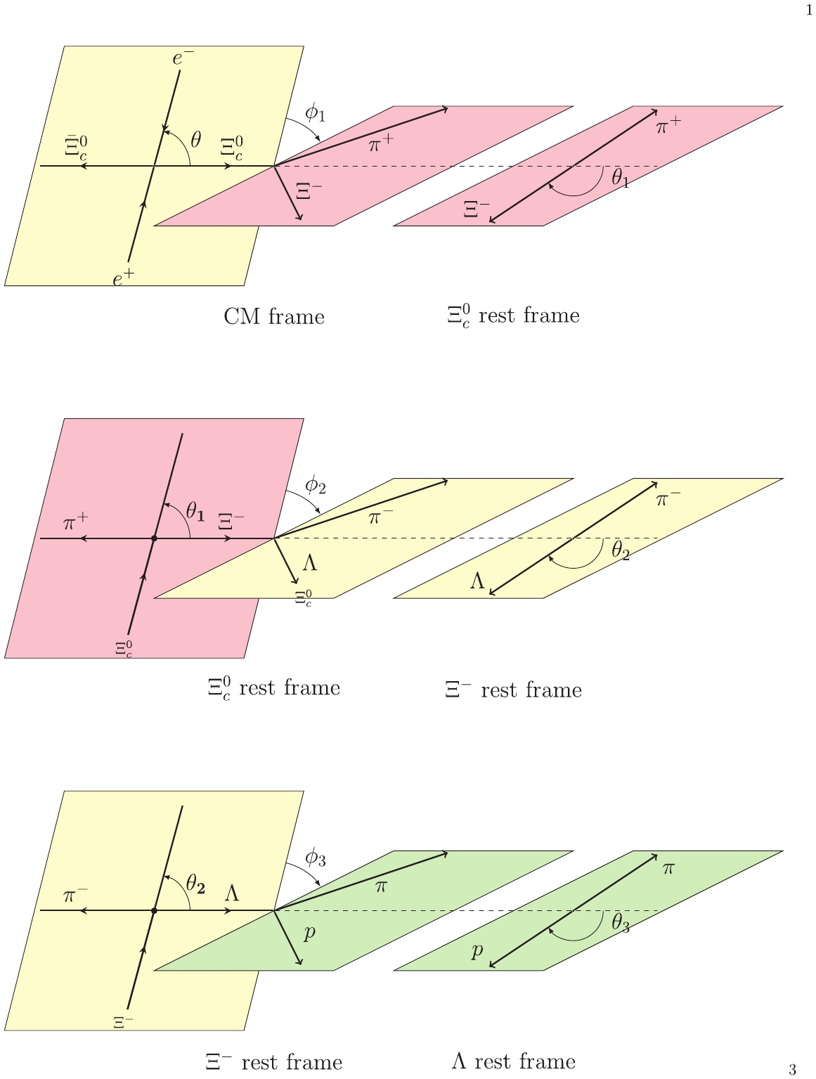
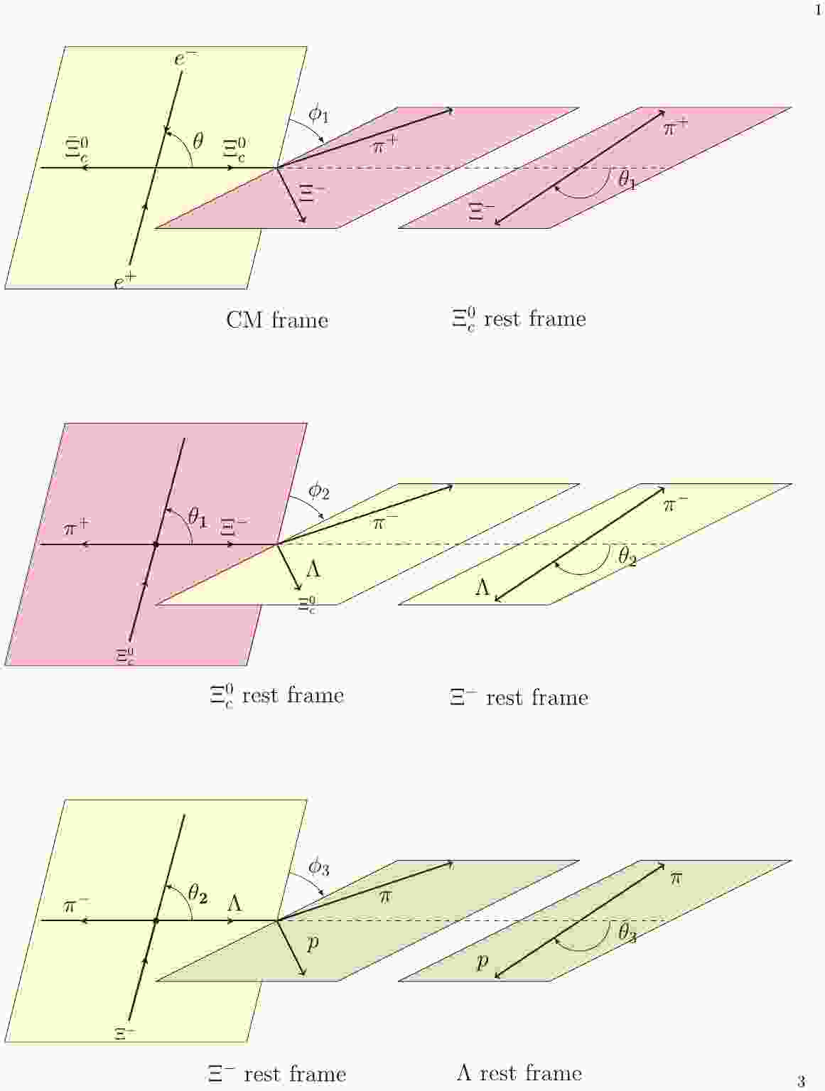
Figure 1. (color online) Definition of helicity frame of
$ e^{+} e^{-}\rightarrow $ $ \Xi_c^{0} \bar{ \Xi}_c ^{0},\Xi_c^{0} \rightarrow $ $\Xi^{-}\pi^{+},\Xi^{-} \rightarrow\Lambda \pi^{-},\Lambda \rightarrow p \pi $ .decay angles amplitude $ e^{+} e^{-} \rightarrow \Xi_c^{0} (\lambda_0)\bar{ \Xi}_c ^{0}(\lambda_1) $ 

( $ \theta,\phi $ )

$ A_{\lambda_0,\lambda_1} $ 

$ \Xi_c^{0} \rightarrow \Xi^{-}(\lambda_2)\pi^{+} $ 

( $ \theta_1,\phi_1 $ )

$ B_{\lambda_2} $ 

$ \Xi^{-} \rightarrow \Lambda(\lambda_3)\pi^{-} $ 

( $ \theta_2,\phi_2 $ )

$ G_{\lambda_3} $ 

$ \Lambda \rightarrow p (\lambda_4)\pi $ 

( $ \theta_3,\phi_3) $ 

$ F_{\lambda_4} $ 

Table 1. Definition of decays, helicity angles, and amplitudes, where
$ \lambda_i $ indicates the helicity values for the corresponding hadron.$ \begin{split} \rho^{\Xi_c}_{\lambda_0,\lambda_0'} =& \displaystyle \sum D^{1*}_{m,\lambda_0-\lambda_1}(\phi,\theta,0)D^{1}_{m,\lambda'_0-\lambda_1}(\phi,\theta,0)\\ &\times A_{\lambda_0,\lambda_1}A^*_{\lambda'_0,\lambda_1}, \end{split}$

(2) where
$ D^{1}_{m,\lambda}(\phi,\theta,0) $ is a Wigner-D function; the sum runs over the virtual photon of spin z-projection,$ m = \pm1 $ . To be more specific, one has$ \begin{split} \rho^{\Xi_c} _{\frac{1}{2},\frac{1}{2}} &= \rho^{\Xi_c}_{-\frac{1}{2},-\frac{1}{2}} = \frac{1}{2} (1+\alpha \cos^2 {\theta }),\\ \rho^{\Xi_c} _{\frac{1}{2},-\frac{1}{2}}& = \rho^{\Xi_c*} _{-\frac{1}{2},\frac{1}{2}} = -\frac{1}{4} i \sqrt{1-\alpha ^2} \sin (2 {\theta }) \sin \left(\Delta _0\right), \end{split} $

(3) where
$ \alpha = \frac{{{{\left| {{A_{1/2, - 1/2}}} \right|}^2} - 2{{\left| {{A_{1/2,1/2}}} \right|}^2}}}{{{{\left| {{A_{1/2, - 1/2}}} \right|}^2} + 2{{\left| {{A_{1/2,1/2}}} \right|}^2}}}$ is the angular distribution parameter of the charmed baryon,$ \Delta_0 $ is the phase angle difference between the two independent helicity amplitudes$ A_{1/2,1/2} $ and$ A_{1/2,-1/2} $ . Here, the spin of$ \bar\Xi_c^0 $ is not observed in the calculation. Then, the degree of$ \Xi_c^0 $ polarization is calculated to be$ \begin{split} {\cal P}^{\Xi_c}_{x} &= {\cal P}^{\Xi_c}_{z} = 0, \\ {\cal P}^{\Xi_c}_{y}& = {\sqrt{1-\alpha ^2} \sin (2 {\theta }) \sin \left(\Delta _0\right)\over 2(1+\alpha \cos^2\theta )}. \end{split} $

(4) The results indicate that in the production x-z plane, the polarization of the charmed baryon vanishes, whereas the TP component normal to the production plane emerges, provided that the factor
$ \sqrt{1-\alpha^2}\sin(\Delta_0) $ has non-zero value. -
We further consider the single tag decay
$ \Xi_c^0\to $ $\Xi^-(\lambda_2)\pi^+ $ and$ \bar\Xi_c^0 $ decays to anything, such that high efficiency is achived. Its helicity amplitude is denoted by$ B_{\lambda_2} $ , and the orientation of$ \Xi^- $ is described by the helicity angles$ (\theta_1,\phi_1) $ . Here,$ \theta_1 $ is defined as the angle between the$ \Xi^- $ momentum in$ \Xi_c^0 $ rest frame and the$ \Xi_c^0 $ momentum in the$ e^+e^- $ center-of-mass (CMS) system, and$ \phi_1 $ is the angle between the$ \Xi^- $ production plane and its decay plane, as shown in Fig. 1.The
$ \Xi_c^0 $ weak decay gives rise to the longitudinal polarization of$ \Xi^- $ by an amount of$ {\cal P}_y^{\Xi_c}\alpha_{\Xi_c} $ along the$ \Xi^- $ flying direction. Hence, this decay can be used to measure the$ \Xi_c $ polarization degree if the decay asymmetry parameter$ \alpha_{\Xi_c} $ is determined. Since the decay violates parity, any difference between the two helicity amplitudes$ B_{\pm1/2} $ characterizes the decay asymmetry distribution. Thus, the decay asymmetry parameter is defined by$\alpha_{\Xi_c} = \left(|B_{+1/2}|^2-\right. $ $\left.|B_{-1/2}|^2\right)\big/ (|B_{+1/2}|^2+|B_{-1/2}|^2) $ . This definition is consistent with the Lee-Yang parameter defined with the S- and P-wave [27].Using the obtained spin density matrix
$ \rho^{\Xi_c} $ , the$ \Xi^- $ spin density matrix is calculated by$ \begin{split} \rho^{\Xi}_{\lambda_2,\lambda_2'} = & \displaystyle\sum_{\lambda_0,\lambda_0'}\rho^{\Xi_c}_{\lambda_0, \lambda'_0}D_{\lambda_0,\lambda_2}^{\frac{1}{2}*}(\phi_{1},\theta_{1},0)D_{\lambda_0',\lambda_2'}^{\frac{1}{2}}\\& \times (\phi_{1},\theta_{1},0)B_{\lambda_2}B_{\lambda'_2}^*, \end{split} $

(5) where
$ D_{\lambda_0,\lambda_2}^{\frac{1}{2}}(\phi_{1},\theta_{1},0) $ is the Wigner-D function.The further simplification yields
$ \begin{split} \rho^{\Xi}_{\frac{1}{2},\frac{1}{2}} \rho^{\Xi}_{-\frac{1}{2},-\frac{1}{2}} =& {1\over 2}(P_0^{\Xi_c}+\alpha_{\Xi_c}P_y^{\Xi_c}\sin\theta_1\sin\phi_1),\\ \rho^{\Xi}_{\frac{1}{2},-\frac{1}{2}} =& \rho^{\Xi*}_{-\frac{1}{2},\frac{1}{2}} = \frac{1}{4}{\rm e}^{{\rm i}\Delta_1}\sqrt{1-\alpha^2_{\Xi_c}}\\ & \times P_y^{\Xi_c}(\cos \theta _1 \sin \phi _1+i \cos \phi _1), \end{split}$

(6) where
$ \Delta_1 $ is the phase angle difference between the two helicity amplitudes$ B_{1/2} $ and$ B_{-1/2} $ , and the$ \Xi_c $ spin polarization components are taken as$ \begin{array}{l} P_0^{\Xi_c} = \rho^{\Xi_c}_{{1\over 2},{1\over 2}}+\rho^{\Xi_c}_{-{1\over 2},-{1\over 2}} = 1+\alpha\cos^2\theta,\\ P_y^{\Xi_c} = -2i {\rm{Im}}(\rho^{\Xi_c}_{{1\over 2},-{1\over 2}}) = -{1\over 2}\sqrt{1-\alpha^2}\sin(2\theta)\sin\Delta_0. \end{array} $

The
$ \Xi^- $ angular distribution is given by the trace of its spin density matrix, namely$ \begin{split} {\cal W}_{\Xi}(\theta,\theta_1,\phi_1)& \propto 1+\alpha \cos^2\theta+\sqrt{1-\alpha ^2} \alpha _{\Xi{\rm c}} \\ &\times \sin\theta \cos\theta \sin \theta _1 \sin \phi _1 \sin \Delta_0. \end{split} $

(7) The above distribution can be understood from the role of
$ \Xi_c^0 $ spin polarimeter, i.e.$ {\cal W}_{\Xi}(\theta,\theta_1,\phi_1) = P_0^{\Xi_c}[ 1+{\cal P}_y^{\Xi_c}\alpha_{\Xi_c}\sin(\theta_1)\sin(\phi_1)], $

(8) where
$ P_0^{\Xi_c} $ is unpolarized cross-section.The spin transfer in the
$ \Xi_c^0 $ decay is twofold. The$ \Xi^- $ transverse polarization entirely originates from the$ \Xi_c^0 $ transverse component, and the decayed$ \Xi^- $ acquires some longitudinal polarization partly from the$ \Xi_c^0 $ transverse polarization, and partly from the weak decay. The elements of its polarization vector are calculated to be$ \begin{array}{l} P^{\Xi}_{x} = \displaystyle{1\over 2}\sqrt{1-\alpha_{\Xi_c}^2}P_y^{\Xi_c}(\sin\Delta_1\cos\phi_1-\cos\Delta_1\cos\theta_1\sin\phi_1),\\ P^{\Xi}_{y} = \displaystyle{1\over 2}\sqrt{1-\alpha_{\Xi_c}^2}P_y^{\Xi_c}(\sin\Delta_1\cos\theta_1\sin\phi_1+\cos\Delta_1\cos\phi_1),\\ P^{\Xi}_{z} = \displaystyle{1\over 2}(\alpha_{\Xi_c}P_0^{\Xi_c}-\sin\theta_1 P_y^{\Xi_c}\sin\phi_1). \end{array} $

(9) -
To optimally use the information available in the experiment, we formulate the joint angular distributions for the full decay chain, namely,
$e^{+} e^{-} \rightarrow \Xi_c^{0} \bar{ \Xi}_c ^{0},\Xi_c^{0} \rightarrow \Xi^{-}\pi^{+}, $ $ \Xi^{-} \rightarrow\Lambda \pi^{-},\Lambda \rightarrow p \pi $ , and$ \bar\Xi_c^0 $ decaying into anything. The first two decay chains have been encoded in the$ \Xi^- $ spin density matrix, and thus allow us to construct the complete decay amplitude beginning with the$ \Xi^- $ decay. Helicity amplitudes for$ \Xi^- $ and$ \Lambda $ decays are given in Table 1, and their decay asymmetry parameters are denoted by$ \alpha_{\Xi} $ and$ \alpha_\Lambda $ , respectively, defined by$\alpha_\Xi = (|G_{1/2}|^2-|G_{-1/2}|^2)/ $ $ |G_{1/2}|^2+|G_{-1/2}|^2, $ and$\alpha_\Lambda = (|F_{1/2}|^2-|F_{-1/2}|^2)/|F_{1/2}|^2+ $ $ |F_{-1/2}|^2 $ . Helicity angles, ($ \theta_2,\phi_2 $ ) for$ \Xi^-\to\Lambda\pi^- $ and$ (\theta_3,\phi_3) $ for$ \Lambda\to p\pi^- $ , are illustrated in Fig. 1. Subsequently, the joint angular distribution for the full decay chain is calculated by$ \begin{split} {\cal W}&(\theta,\theta_1,\theta_2,\theta_3,\phi_1,\phi_2,\phi_3) \propto \displaystyle\sum _{\lambda_i,\lambda_j = \pm \frac{1}{2}} \rho^{\Xi}_{\lambda_2,\lambda_2'}(\theta,\theta_1,\phi_1)\\ &\times D_{\lambda_2,\lambda_3}^{\frac{1}{2}}(\phi_2,\theta_2,0)D_{\lambda_2',\lambda_3'}^{\frac{1}{2}*}(\phi_2,\theta_2,0) \\ &\times D_{\lambda_3,\lambda_4}^{\frac{1}{2}}(\phi_3,\theta_3,0)D_{\lambda_3',\lambda_4}^{\frac{1}{2}*}(\phi_3,\theta_3,0) \\ &\times G_{\lambda_3}^*G_{\lambda_3'}|F_{\lambda_4}|^2. \end{split} $

(10) After the
$ \phi_3 $ angle is integrated out, the simplified expression in terms of decay asymmetry parameters is given by$ \begin{split} {\cal W}&(\theta,\theta_1,\theta_2,\theta_3,\phi_1,\phi_2) \propto {\cal W}_{\Xi}(1+\alpha_\Lambda\alpha_\Xi\cos\theta_3)\\ &+(\alpha_\Lambda\cos\theta_3+\alpha_\Xi)(P^\Xi_x\sin\theta_2\cos\phi_2\\ &-P^\Xi_y\sin\theta_2\sin\phi_2+P^\Xi_z\cos\theta_2). \end{split} $

(11) If we do not observe the angular distributions for the last step decay, we integrate out the angle
$ \theta_3 $ . Then, we have a reduced distribution in terms of the$ \Xi $ spin polarization as$ \begin{split} {\cal W}_\Lambda&(\theta,\theta_1,\theta_2,\phi_1,\phi_2) \propto {\cal W}_{\Xi}+\alpha _{\Xi}P_z^\Xi\cos\theta_2\\ &+\alpha_\Xi\sin\theta_2(P_x^\Xi\cos\phi_2-P_y^\Xi\sin\phi_2). \end{split}$

(12) -
The transverse polarization of charmed baryon is spontaneously generated from the
$ e^+e^- $ annihilation, which is characterized by Eq. (4). The charmed baryon carries a reverse polarization degree in the detector of the east and west region, and it has a net-zero degree of polarization in the full coverage of detector. To display its distribution relative to$ \cos\theta $ in the data analysis, a general way is to fill the distribution of$ \langle \sin\theta_1\sin\phi_1\rangle $ relative to$ \cos\theta $ , which makes it independent of the measurement of the angular distribution parameter$ \alpha $ . Here, the average is defined by$ \begin{split} \langle \sin\theta_1\sin\phi_1\rangle & = {1\over N} \displaystyle\int {\cal W}_\Xi(\theta,\theta_1,\phi_1)\sin\theta_1\sin\phi_1{\rm d}(\cos\theta_1){\rm d}\phi_1\\ & = {1\over 3}{\cal P}_y^{\Xi_c}\alpha_{\Xi_c}, \end{split} $

(13) with a normalization factor
$ N = \int {\cal W}_\Xi(\theta,\theta_1,\phi_1){\rm d}(\cos\theta_1){\rm d}\phi_1. $

A Monte-Carlo (MC) simulation is performed to generate events using Eq. (7), with a naive choice of parameters
$ \alpha _{\Xi_c} = -0.1,\; \alpha = 0.3 $ . Thus, we fill a histogram of$ \cos\theta $ with a weight of$ \sin\theta_1\sin\phi_1/N $ as shown in Fig. 2, here N is the number of generated events. With a sufficient size of MC sample, one can see that the filled distribution of$ \langle\sin\theta_1\sin\phi_1\rangle $ relative to$ \cos\theta $ can be described with the$ {\cal P}^{\Xi_c}_y $ distribution, as given by Eq. (4).
Figure 2.
$ \langle\sin\theta_1\sin\phi_1\rangle $ distribution versus$ \cos\theta $ . Dots with error bars are filled with 1.0 million MC events, and the curve depicts a comparison with the charmed baryon transverse polarization$ {\cal P}^{\Xi_c}_y $ . -
To measure the decay asymmetry parameter
$ \alpha_{\Xi_c} $ , we make use of the decay chain to the greatest degree possible. The precise measurement benefits from the full decay chain of polarization information, which is expressed in terms of hyperon$ \Xi $ and$ \Lambda $ weak decays. We assume that the$ \alpha_{\Xi_c} $ parameter is extracted from fitting the normalized angular distribution$ {\widetilde{\cal W}}(\theta,\theta_1,\theta_2,\theta_3,\phi_1,\phi_2) $ , defined by$W\left(\theta,\theta_1,\theta_2,\right.\left.\theta_3,\phi_1,\phi_2\right) / \int\cdots\int W(\cdots) {\rm d}\cos\theta {\rm d}\cos\theta_1 {\rm d}\cos\theta_2 $ ${\rm d}\cos\theta_3 {\rm d}\phi_1 {\rm d}\phi_2 $ , to data event by event with a likelihood function$ L = \mathop \prod \limits_{i = 1}^N {\widetilde{\cal W}}(\theta,\theta_1,\theta_2,\theta_3,\phi_1,\phi_2,\alpha_{\Xi_c}), $

(14) where N is the number of observed events. The statistical sensitivity associated to the parameter estimation with the maximum likelihood method is determined by the relative uncertainty
$ \delta(\alpha_{\Xi_c}) = \frac{\sqrt{V(\alpha_{\Xi_c})}}{|\alpha_{\Xi_c}|}, $

(15) where
$ V(\alpha_{\Xi_c}) $ denotes the variance of the parameter$ \alpha _{\Xi_c } $ , which can be determined by$ \begin{split} V^{-1}(\alpha_{\Xi_c}) = & N\int \frac{1}{{\widetilde{\cal W}}(\theta_{i},\phi_i,\alpha _{\Xi_c })} \left[\frac{\partial{\widetilde{\cal W}} (\theta_{i},\phi_i,\alpha _{\Xi_c })}{\partial \alpha _{\Xi_c }}\right]^2\\ &\times \prod\limits_{i} {{\rm d}\cos\theta_i}\prod\limits_{j}{\rm d}\phi_j. \end{split} $

(16) To obtain the dependence of sensitivity on the signal yields N, we estimate the value of
$ \delta(\alpha_{\Xi_c}) $ by taking the parameters [28] as$ \alpha _{\Xi } = -0.392\pm0.008, \alpha _{\Lambda} = 0.750\pm0.010, $ whereas no measurement is available for the$ \Xi_c $ angular distribution parameter, we naively assume$ \alpha = 0.6 $ . The parameter$ \alpha _{\Xi_c } $ sensitivity is calculated as follows:$ \frac{0.251^{+0.002}_{-0.008}}{\sqrt N} < \delta(\alpha _{\Xi_c })<\frac{1.943^{+0.066}_{-0.012}}{\sqrt N}, $

(17) where the uncertainties due to the
$ \alpha _{\Xi } $ and$ \alpha _{\Lambda} $ uncertainties, and the lower and upper bonds are determined by taking the$ \alpha_{\Xi_c} = -0.1 $ and$ -0.9 $ , respectively. Here, uncertainties are due to the$ \alpha _{\Xi } $ and$ \alpha _{\Lambda} $ uncertainties.Regarding other
$ \alpha_{\Xi_c} $ values, we plot the sensitivity versus the$ \Xi_c $ statistics, as shown in Fig. 3, where the experimental effects, such as the backgrounds and the detection angular acceptance, are not taken into consideration. If we take$ \alpha_{\Xi_c} = -0.6\pm0.4 $ for the$ \Xi_c^0\to\Xi^-\pi^+ $ decay, the signal 50000 events yields sensitivity of this parameter reaching the precision of$ 0.1\sim0.9 $ %. The$ \alpha_{\Xi_c} $ measurement can be performed in the super KEKB, or in the future Super Tau Charm Facility, which was proposed by Chinese and Russian physicists, with the center-of-mass energy from 2 to 5 GeV.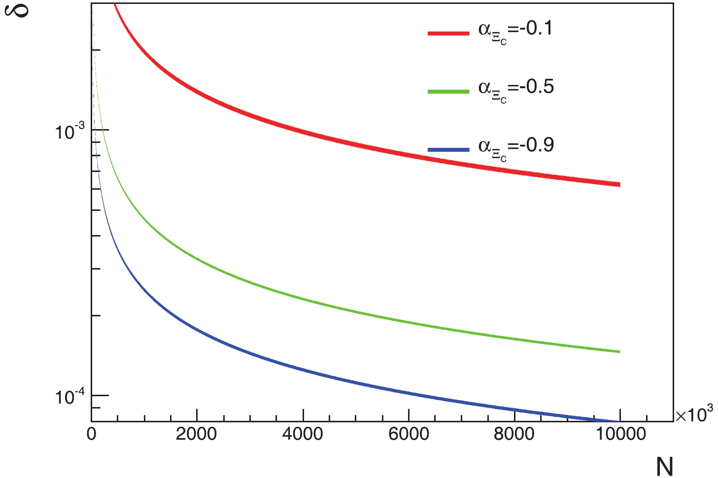
Figure 3. (color online) The
$ \alpha_{\Xi_c} $ sensitivity relative to signal yields N in terms of different value$ \alpha_{\Xi_c} $ . Curves from top to bottom correspond to$ \alpha_{\Xi_c} $ values of -0.1, -0.5, and -0.9, respectively. -
We formulate the polarization in the process
$ e^+e^-\to\Xi_c^0\bar\Xi_c^0 $ motivated by the study of weak asymmetry decay parameters for the$ \Xi_c\to\Xi\pi $ decay. As in other continuum process, the transverse polarization may be spontaneously generated accompanied by the baryon pair production from$ e^+e^- $ annihilations. We formulate the decay asymmetry parameter for the weak decay$ \Xi_c\to\Xi\pi $ , and we show how the transverse polarization is transferred from the charmed baryon to the decayed$ \Xi $ hyperon. Taking advantage of the full decay chain, we formulate the joint angular distributions for the decay chain$ \Xi\to\Lambda\pi $ and$ \Lambda\to p\pi^- $ . A Monte-Carlo simulation is performed to show how to display the transverse polarization effects. The sensitivity to measure the$ \alpha_{\Xi_c} $ asymmetry parameters is estimated with the full decay chain formula.
Polarization in ${{ \Xi_c^0}}$ decays
- Received Date: 2019-07-21
- Accepted Date: 2019-09-27
- Available Online: 2020-01-01
Abstract: Measurements of decay asymmetry parameters of charmed baryons, e.g.,


 DownLoad: