


 Abstract
 HTML
HTML Reference
 Related
 PDF
PDF


-
Lattice QCD is a gauge invariant and nonperturbative regularization scheme for QCD that was introduced by K. Wilson in 1974 [1]. Many quantities can be obtained from the first principles by using a finite space-time lattice to simulate the interactions between quarks and gluons. The calculation of diagrams with disconnected quark loops is one of the most challenging problems in lattice QCD. Disconnected loops are needed in calculations of many lattice QCD observables, such as the nucleon electromagnetic form factors [2, 3], pi-NN coupling and pion polarizability [4], the mass of pseudoscalar flavor-singlet mesons [5, 6], strangeness and charm content of the nucleon [7, 8], hadronic scattering lengths and structure functions [9], and electron or muon hadronic
$ g-2 $ loop contributions [10]. In the lattice QCD, the expectation value of disconnected quark loops can be written as [11]$ \left\langle \overline{\psi}\varGamma\psi\right\rangle = -{\rm{Tr}}\left(\varGamma M^{-1}\right), $

(1) where
$ \varGamma\in\left\{ 1,\thinspace\gamma_{\mu},\thinspace\gamma_{5},\thinspace\gamma_{5}\gamma_{\mu},\thinspace\sigma_{\mu\nu\thinspace},\mu,\nu = 1,2,3,4\right\} $ , and M is the Dirac fermion operator. In this work, we use Wilson's Dirac operator, which can be written as$ M = {1}-\kappa D,\quad\kappa = \frac{1}{2\left(am+4\right)}, $

(2) $ \begin{split} D{{\left( n|m \right)}_{\begin{smallmatrix} \alpha \beta \\ ab \end{smallmatrix}}} =& \sum\limits_{\mu = 1}^{4}{{{\left( 1-{{\gamma }_{\mu }} \right)}_{\alpha \beta }}{{U}_{\mu }}{{\left( n \right)}_{ab}}{{\delta }_{n+\widehat{\mu },m}}} \\ & +\sum\limits_{\mu = 1}^{4}{{{\left( 1+{{\gamma }_{\mu }} \right)}_{\alpha \beta }}{{U}_{-\mu }}{{\left( n \right)}_{ab}}{{\delta }_{n-\widehat{\mu },m}}}, \end{split}$

(3) where a is the lattice spacing, and D is referred to as the hopping matrix. The real number
$ \kappa $ is the hopping parameter [12]. To calculate the disconnected diagrams, we need to solve the equation$ Mx = b, $

(4) where M is the Dirac matrix with dimension
$ K\times K $ , and b is the source vector of dimension$ K\times1 $ . The solution of this equation is$ x = M^{-1}b. $

(5) The evaluation of disconnected quark loops requires
$ M^{-1} $ connecting arbitrary pairs of lattice points. Generally, Wilson's Dirac matrix is a large sparse matrix and its typical dimension K is from$ 10^{6} $ up to$ 10^{9} $ . Its direct evaluation is prohibitively expensive, both in terms of computer time and memory.In order to calculate disconnected quark loops, specific techniques must be introduced. Unbiased noise methods are traditionally used to estimate the inverse matrix [13, 14]. The truncated solver method (TSM) [15] and the spin explicit method (SEM) [16, 17] were introduced to reduce the stochastic error. A probing technique is also a way to deal with this problem [18]. However, we found that all stochastic methods result in large errors in the calculations of disconnected quark loops
$ {\rm{Tr}}\left(\varGamma M^{-1}\right) $ . Hence, we introduce the symmetric multi-probing source (SMP) method to calculate all disconnected quark loops, and compare the results with the$ Z\left(2\right) $ noise and spin-color explicit (SCE) methods. All comparisons are based on the point source results which are taken as exact. -
In general, the inverse of a large sparse matrix can be calculated by using the unbiased stochastic method. Here, we briefly review the
$ Z\left(2\right) $ noise method. We assume L column noise vectors$ b^{1} $ ,$ b^{2} $ ,$ b^{3} $ ,$ \ldots $ ,$ b^{L} $ , which have the following two properties [13],$ \left\langle b_{i}\right\rangle = \frac{1}{L}\sum\limits_{l = 1}^{L}b_{i}^{l} = {\cal O}\left(1/\sqrt{L}\right), $

(6) $ {\left\langle b_{i}b_{j}\right\rangle = \frac{1}{L}\sum\limits_{l = 1}^{L}b_{i}^{l}b_{j}^{l} = \delta_{ij}+{\cal O}\left(1/\sqrt{L}\right),} $

(7) where
$ b_{i}^{l} $ is the$ i $ -th entry in the noise vector l. The stochastic average$ <\cdot\cdot\cdot> $ is taken over the ensemble of noise vectors L.$\rm{If}\, Z\left(2\right) $ noise vectors are used in Eq. (4), we obtain$ x_{i}^{l} = \sum\limits_{k}M_{ik}^{-1}b_{k}^{l}. $

(8) The inverse matrix element,
$ M_{ij}^{-1} $ , is given as$ <b_{j}x_{i}> = \sum\limits_{k}M_{ik}^{-1}<b_{j}b_{k}> = M_{ij}^{-1}. $

(9) The variance of the
$ Z(2) $ noise method is [19]$ \sigma^{2}\equiv\frac{1}{L}\sum\limits_{i\neq j}^{K}\left|M_{ij}^{-1}\right|^{2}. $

(10) It can be seen that the stochastic error of the
$ Z\left(2\right) $ noise estimate results only from the off-diagonal elements of the inverse matrix.Therefore, we obtain
$ {\rm{Tr}}(\varGamma M^{-1}) $ $ \begin{split} {\rm{Tr}}\left(\varGamma M^{-1}\right) = & \sum\limits_{j}\varGamma M_{jj}^{-1} = \sum\limits_{i,j}\varGamma M_{ij}^{-1}\delta_{ij} \\ =& \sum\limits_{i,j}\frac{1}{L}\sum\limits_{l}\varGamma M_{ij}^{-1}b_{i}^{l}b_{j}^{l} = \sum\limits_{i}\frac{1}{L}\sum\limits_{l}b_{i}^{l}\left(\varGamma x_{i}^{l}\right). \end{split} $

(11) In order to reduce the error of the
$ Z\left(2\right) $ noise method, we applied an independent stochastic inversion of the spin and color components (spin-color explicit method, SCE method) for each$ Z\left(2\right) $ noise vector, similar to SEM [16]. -
The SMP source vector
$ \phi_{P} $ is introduced as follows [20]$ \phi_{P}\left(S(x,P),\alpha,a\right) = \sum\limits_{y\in S(x,P)}\psi\left(y,\alpha,a\right), $

(12) where
$ \alpha $ is the Dirac index and a the color index.$ S(x,P) $ represents the sites with the same color of x obtained by the symmetric coloring scheme$ P\left(\dfrac{n_{\rm s}}{d},\dfrac{n_{\rm s}}{d},\dfrac{n_{\rm s}}{d},\dfrac{n_{\rm t}}{d},{mode}\right) $ , where$ n_{\rm s} $ and$ n_{\rm t} $ are the spatial and temporal sizes of the lattice. d is the distance parameter, and$ mode = 0,1,2 $ corresponds to the Normal, Split and Combined mode. x is the seed site at$ \left(x_{1},x_{2},x_{3},x_{4}\right) $ and y are the other lattice sites belonging to the set$ S(x,P) $ .$ \psi $ is the normalized point source vector. The number of SMP sources$ N_{{\rm SMP}} $ that cover all lattice sites is$ {N_{{\rm{SMP}}}} = \left\{ {\begin{array}{*{20}{l}} {12{d^4}}&{mode = 0,}\\ {24{d^4}}&{mode = 1,}\\ {6{d^4}}&{mode = 2.} \end{array}} \right.$

(13) Applying the SMP source in Eq. (4) to calculate the trace of
$ \varGamma M^{-1} $ , we obtain$\begin{split} {\rm{Tr}}\left(\varGamma M^{-1}\right)_{{\rm SMP}} = & \sum\limits_{x,\alpha,a}\psi\left(x,\alpha,a\right)\left(\varGamma M^{-1}\right)\phi_{P}\left(S\left(x,P\right),\alpha,a\right) \\ =& \sum\limits_{x,\alpha,a}\psi\left(x,\alpha,a\right)\left(\varGamma M^{-1}\right)\psi\left(x,\alpha,a\right) +\sum\limits_{y\in S\left(x,P\right)}^{y\neq x}\sum\limits_{\alpha,a}\psi\left(x,\alpha,a\right)\left(\varGamma M^{-1}\right)\psi\left(y,\alpha,a\right) \\ =& {\rm{Tr}}\left(\varGamma M^{-1}\right)+\sum\limits_{y\in S\left(x,P\right)}^{y\neq x}\sum\limits_{\alpha,a}\psi\left(x,\alpha,a\right)\left(\varGamma M^{-1}\right)\psi\left(y,\alpha,a\right), \end{split} $

(14) where the second term in the last line is the sum of off-diagonal elements of
$ \varGamma M^{-1} $ . Considering the space-time locality of M, this term can be regarded as the error in the calculation of$ {\rm{Tr}}\left(\varGamma M^{-1}\right) $ . If we choose the proper scheme P of the SMP source, the error is quite small. In this case, we can neglect the error term and get$ {\rm{Tr}}\left(\varGamma M^{-1}\right)\approx {\rm{Tr}}\left(\varGamma M^{-1}\right)_{{\rm SMP}}. $

(15) -
It is very time consuming to solve Eq. (4) if b is the point source (p-s) vector which runs over all lattice sites of a large lattice. In this work, we use the point source method to evaluate
$ {\rm{Tr}}\left(\varGamma M^{-1}\right) $ , and take the result as exact, and use it for comparison. We only work with ensembles of Iwasaki pure gauge configurations, where the volume is$ L_{\sigma}^{3}\times L_{\tau} =$ $ 12^{3}\times24 $ . The lattice spacing of the ensembles is$ a\approx 0.1 $ fm. The analysis is performed on$ 25 $ configurations with$ \kappa = 0.151 $ , corresponding to$ m_\pi\approx 488 $ MeV. We show the results for$ {\rm{Tr}}\left(M^{-1}\right) $ and$ {\rm{Tr}}\left(\gamma_{5}M^{-1}\right) $ in the main body of this paper. The results for$ {\rm{Tr}}\left(\gamma_{3}M^{-1}\right) $ ,$ {\rm{Tr}}\left(\gamma_{5}\gamma_{1}M^{-1}\right) $ and$ {\rm{Tr}}\left(\sigma_{34}M^{-1}\right) $ , selected as representative, are presented in appendix A.Using the identity
$ M = \gamma_{5}M^{\dagger}\gamma_{5} $ [21], we obtain$\begin{split} {\rm{Tr}}\left(\gamma_{5}M^{-1}\right) =& {\rm{Tr}}\left(\gamma_{5}\gamma_{5}\left(M^{-1}\right)^{\dagger}\gamma_{5}\right) \\ =& {\rm{Tr}}\left(\left(M^{-1}\right)^{\dagger}\gamma_{5}\right) = {\rm{Tr}}\left(\left(\gamma_{5}M^{-1}\right)^{\dagger}\right). \end{split}$

(16) Therefore,
$ {\rm{Tr}}\left(\gamma_{5}M^{-1}\right) $ is a real number, and$ {\rm{Tr}}\left(M^{-1}\right) $ is also real. The absolute error$ \Delta r $ discussed in this work is defined as$ \Delta r = \left|r_{p}-r_{m}\right|,\thinspace\thinspace\thinspace\thinspace\thinspace\thinspace\thinspace\thinspace $

(17) where
$ r_{p} $ is the result for the point source and$ r_{m} $ is the result for any other method.We also define the method error
$ \sigma $ as$ \sigma^{2} = \frac{1}{N_{\rm{conf}}(N_{\rm{conf}}-1)}\sum\limits_{i = 1}^{N_{\rm{conf}}}\Delta r_{i}^{2}. $

(18) $ \Delta {{r}_{i}} $ is the absolute error of the i-th configuration (conf), and$ N_{\rm{conf}} $ is the number of configurations. In the definition of$ \sigma $ , we use$ r_{p} $ and not the average value$ \left\langle r\right\rangle _{c} $ of all configurations, to eliminate the fluctuations due to different configurations. Therefore, this definition gives only the error of the method. -
The results and absolute errors of the first ten configurations are shown as representative in this paper. However, we show the method error for all 25 configurations. For the SMP method, the results for
$ {\rm{Tr}}\left(M^{-1}\right) $ are shown in Table 1, and in Table 2 for$ {\rm{Tr}}\left(\gamma_{5}M^{-1}\right) $ . The number of source vectors for all methods is the same.conf. p-s $N=15552\thinspace\left(6,0\right)$ 

$N=3072\thinspace\left(4,0\right)$ 

$N=1536\thinspace\left(4,2\right)$ 

$N=384\thinspace\left(2,1\right)$ 

$N=192\thinspace\left(2,0\right)$ 

$N=96\thinspace\left(2,2\right)$ 

1 453821.05 453821.93 453834.19 453831.06 453821.88 453785.60 453890.51 2 454042.56 454049.54 454036.58 454040.99 454020.87 453919.91 453945.70 3 454216.18 454218.24 454219.28 454218.60 454223.99 454389.67 454395.52 4 454002.41 453999.82 453998.76 453994.74 453964.91 454033.19 454069.26 5 454354.48 454357.04 454337.75 454319.32 454291.41 454229.23 454220.83 6 454301.64 454299.51 454308.33 454298.46 454274.90 454210.82 454231.96 7 454085.53 454087.16 454089.11 454085.17 454083.09 454065.35 454038.91 8 454059.63 454060.60 454054.26 454053.96 454016.87 454104.69 454054.37 9 453944.56 453941.69 453936.50 453930.76 453919.66 453778.34 453765.85 10 453914.30 453915.53 453924.14 453923.83 453936.33 453826.90 453825.25 Table 1. Results for
$\mathrm{Tr}\left(M^{-1}\right)$ for the SMP method. N is the number of SMP source vectors. The numbers in the parentheses represent the parameters d and$mode$ of the SMP source; for example,$\left(6,0\right)$ denotes$d=6$ and$mode=0$ . The SMP method is a good approximation when the number of source vectors is large.
Figure 1. (color online) Absolute error of
${\rm{Tr}}\left(M^{-1}\right)$ for the SMP method. The numbers in the parentheses represent the parameters d and$mode$ of the SMP source vectors; for example,$\left(6,0\right)$ denotes$d = 6$ and$mode = 0$ .conf. p-s $N=15552\thinspace\left(6,0\right)$ 

$N=3072\thinspace\left(4,0\right)$ 

$N=1536\thinspace\left(4,2\right)$ 

$N=384\thinspace\left(2,1\right)$ 

$N=192\thinspace\left(2,0\right)$ 

$N=96\thinspace\left(2,2\right)$ 

1 −18.94 −18.37 −22.18 −15.61 −10.08 −21.66 −22.73 2 202.86 203.21 202.90 212.26 192.83 184.64 188.23 3 183.32 184.33 181.43 180.09 178.41 178.20 148.52 4 −170.65 −170.89 −163.42 −160.16 −186.75 −172.39 −206.26 5 −586.77 −583.80 −563.81 −555.51 −559.26 −569.70 −519.76 6 74.85 73.18 73.35 75.99 81.00 96.71 124.26 7 −288.10 −290.81 −288.23 −284.46 −291.66 −280.63 −271.28 8 141.12 141.86 137.16 138.44 153.09 167.57 164.22 9 −338.58 −335.66 −342.16 −329.44 −338.10 −332.02 −351.82 10 −223.22 −220.96 −224.15 −221.93 −237.32 −218.63 −222.10 Table 2. Results for
$\mathrm{Tr}\left(\gamma_{5}M^{-1}\right)$ for the SMP method. N is the number of SMP source vectors. The numbers in the parentheses represent the parameters d and$mode$ of the SMP source.
Figure 2. (color online) Absolute error of
${\rm{Tr}}\left(M^{-1}\right)$ for the$Z(2)$ noise method.$N_Z$ is the number of$Z\left(2\right)$ source vectors.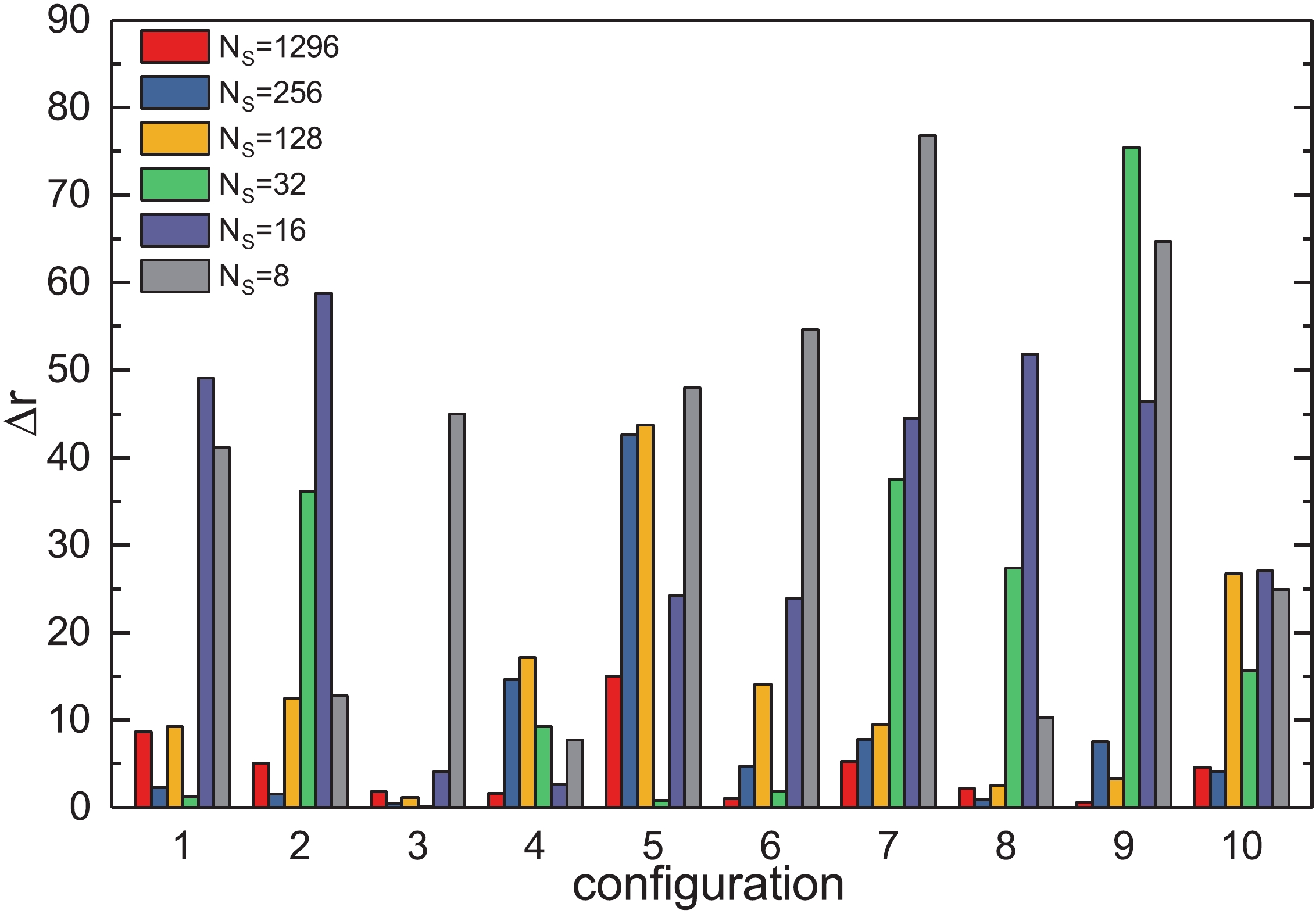
Figure 3. (color online) Absolute error of
${\rm{Tr}}\left(M^{-1}\right)$ for the SCE method.$N_S$ is the number of SCE source vectors.
Figure 4.
(color online) $\sigma$ of${\rm{Tr}}\left(M^{-1}\right)$ as a function of the number of source vectors N for the three different methods.In Figs. 1, 2 and 3, the absolute errors of
$ {\rm{Tr}}\left(M^{-1}\right) $ for the SMP,$ {Z\left(2\right)} $ noise and SCE methods are shown. As expected, as the number of source vectors increases, the absolute errors become smaller for all three methods.In Fig. 4,
$ \left\langle \Delta r \right\rangle $ of$ {\rm{Tr}}\left(M^{-1}\right) $ for the SMP and SCE methods are compared with the$ {{Z}}\left(2\right) $ noise method for the same number of source vectors, indicating that when the number of source vectors is small, the absolute errors of SMP and SCE are larger than of$ { Z\left(2\right)} $ . The figure also shows that the SCE method does not bring any improvement in the evaluation of the scalar disconnected quark loops compared with the$ {Z\left(2\right)} $ noise method. Hence, the$ Z\left(2\right) $ noise method is an efficient method for the calculation of$ {\rm{Tr}}\left(M^{-1}\right) $ .As the number of source vectors increases, the results of the SMP, SCE and
$ {Z\left(2\right)} $ noise methods become more and more accurate. The results for$ {\rm{Tr}}\left(M^{-1}\right) $ show that the$ {Z\left(2\right)} $ noise method is a good choice for evaluating the scalar disconnected loops.The results for
$ {{\rm{Tr}}}\left(\gamma_{5}M^{-1}\right) $ for the SMP method are shown in Table 2. The absolute errors of$ {{\rm{Tr}}}\left(\gamma_{5}M^{-1}\right) $ are presented in Figs. 5, 6 and 7. As the number of source vectors increases, the absolute errors of all methods decrease, as expected. Fig. 6 shows that the$ Z\left(2\right) $ noise method gives a too large error of$ {\rm{Tr}}\left(\gamma_{5}M^{-1}\right) $ , especially for small N.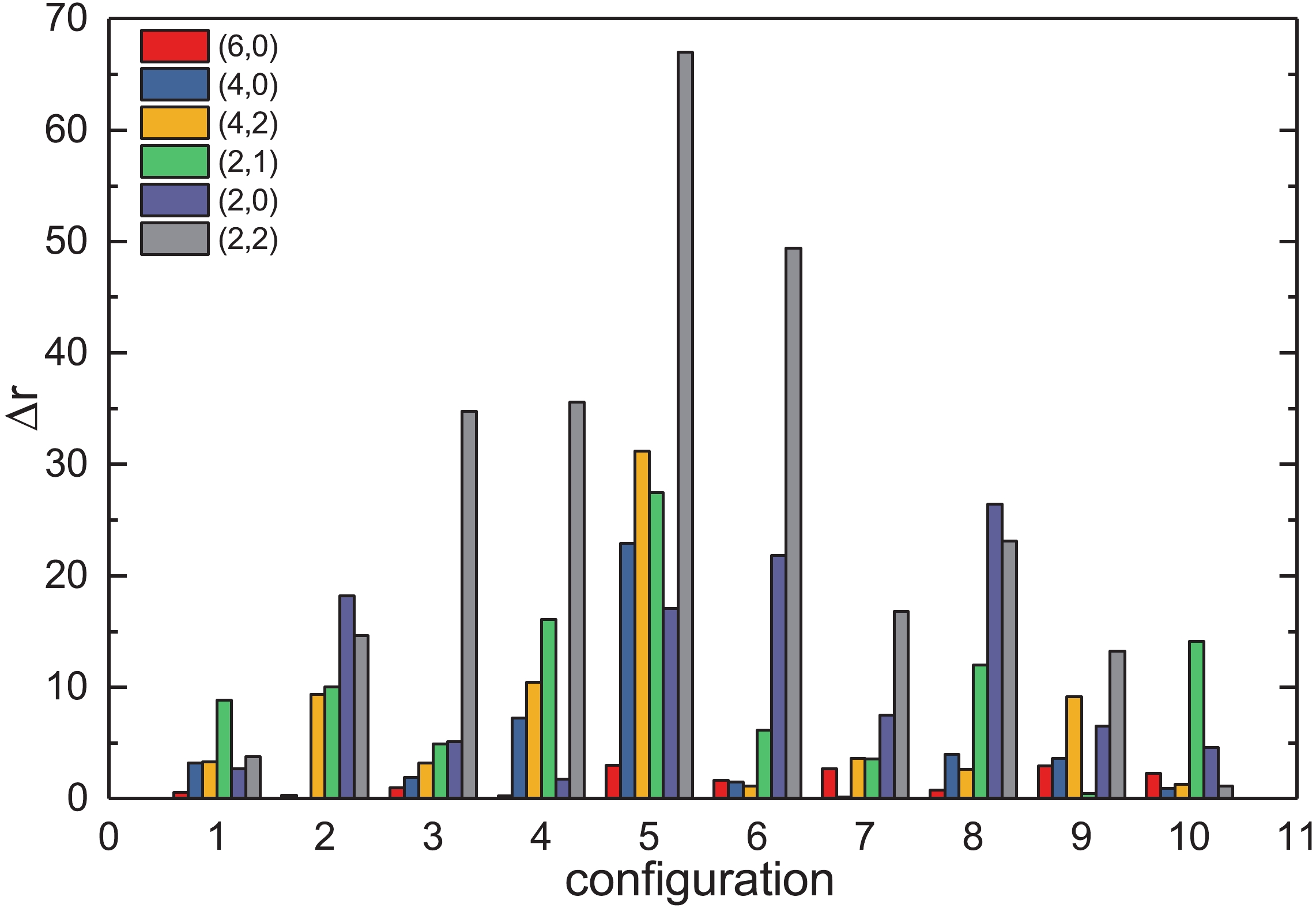
Figure 5. (color online) Absolute error of
${\rm{Tr}}\left(\gamma_{5}M^{-1}\right)$ for the SMP method.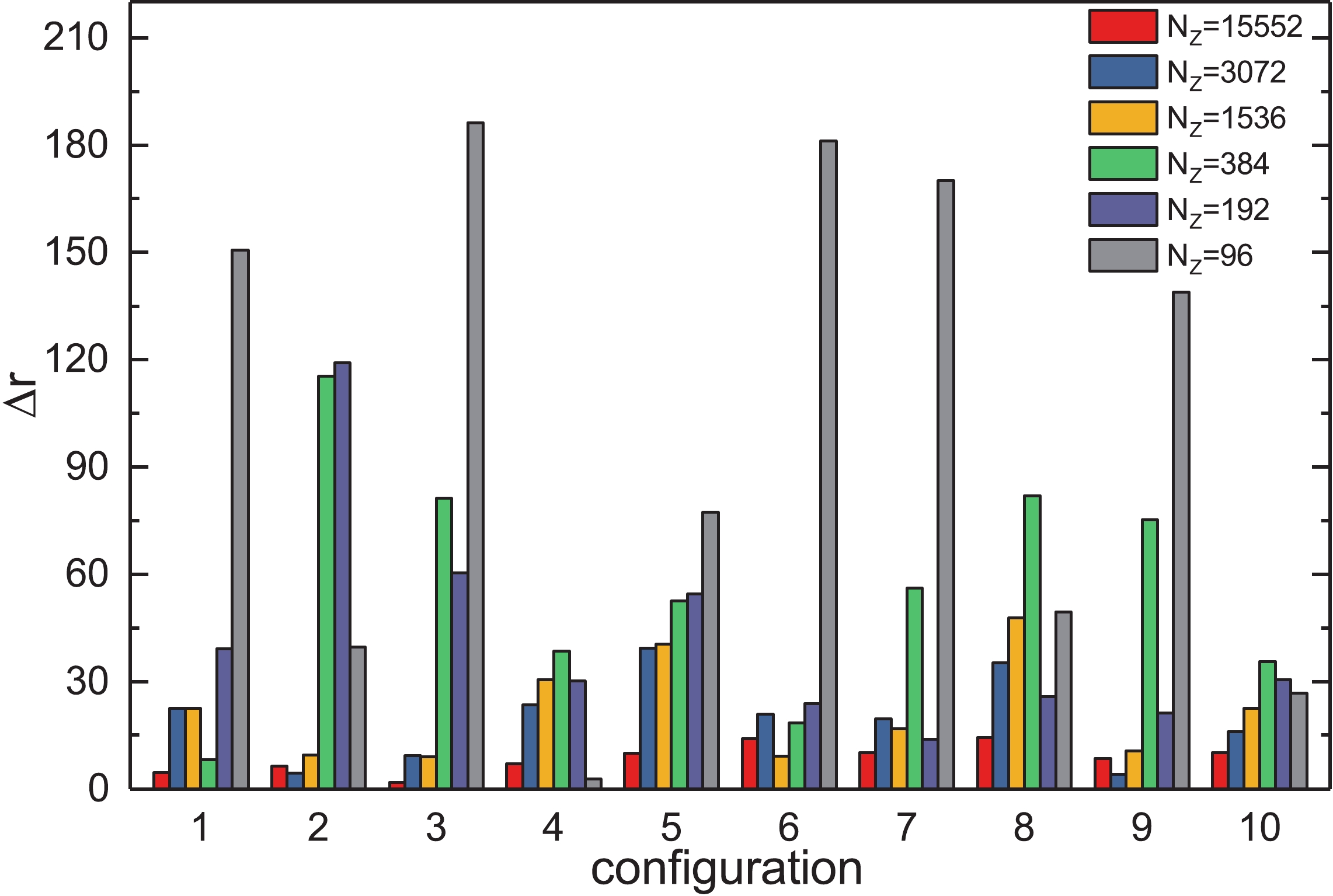
Figure 6. (color online) Absolute error of
${\rm{Tr}}\left(\gamma_{5}M^{-1}\right)$ for the$Z\left(2\right)$ noise method.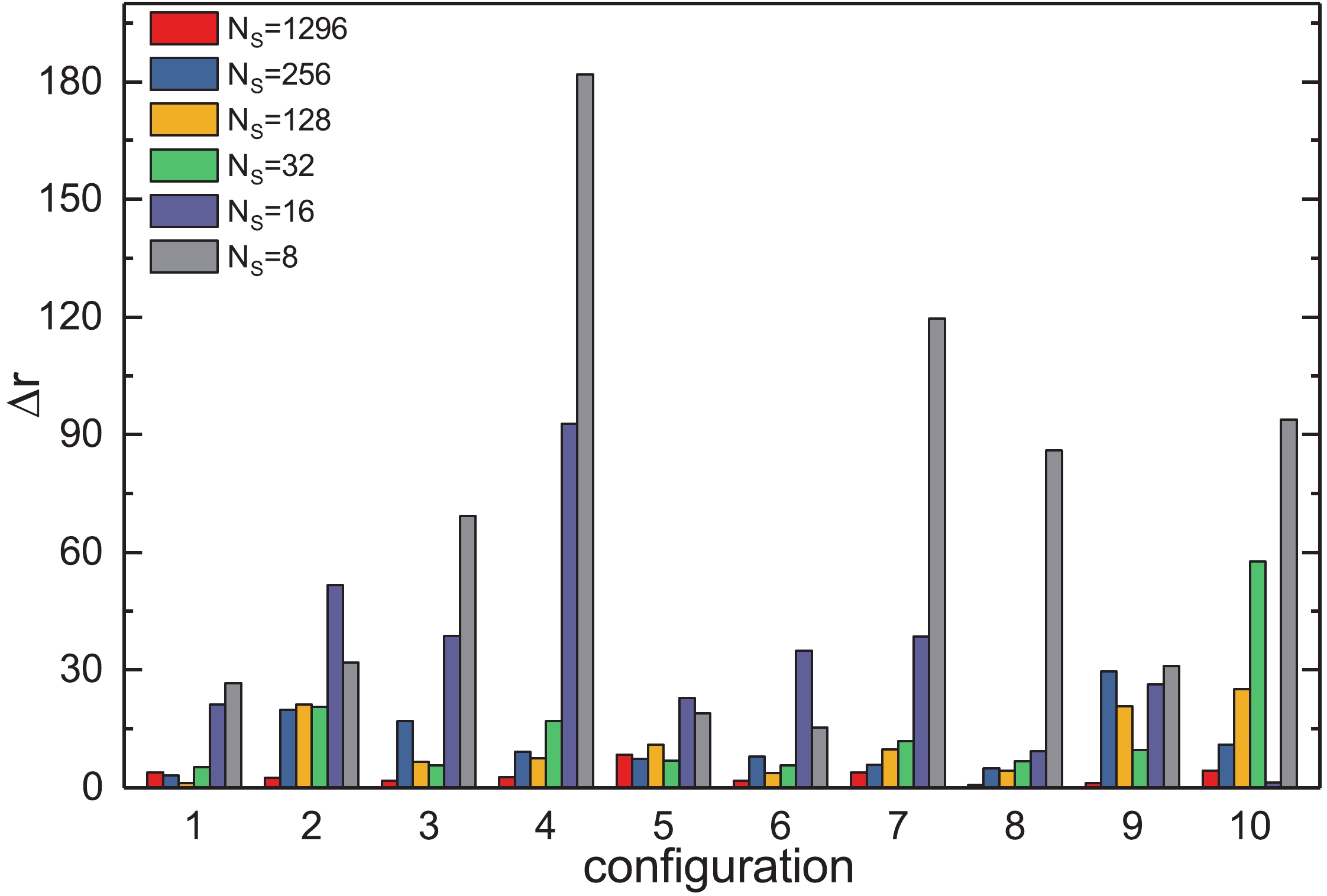
Figure 7. (color online) Absolute error of
${\rm{Tr}}\left(\gamma_{5}M^{-1}\right)$ for the SCE method.In Fig. 8, the method error of
$ {{\rm{Tr}}}\left(\gamma_{5}M^{-1}\right) $ is shown, indicating that$ \sigma $ decreases with increasing number of source vectors for all three methods. The SCE method results in a smaller$ \sigma $ than the$ Z\left(2\right) $ noise method for the same number of source vectors. Hence, the SCE method is an obvious improvement compared with the$ {Z\left(2\right)} $ noise method. Also, the SMP method gives a much smaller method error than the$ Z\left(2\right) $ noise method, especially for a small number of source vectors.
Figure 8. (color online) Method error of
${{\rm{Tr}}}\left(\gamma_{5}M^{-1}\right)$ as a function of the number of source vectors N.All these results indicate that the
$ Z\left(2\right) $ noise method gives a larger error than the SMP and SCE methods for the same number of source vectors in the calculation of$ {{\rm{Tr}}}\left(\gamma_{5}M^{-1}\right) $ . Compared with the$ Z\left(2\right) $ method, the SCE method indeed improves the calculation of$ {{\rm{Tr}}}\left(\gamma_{5}M^{-1}\right) $ . On the other hand, the absolute errors of the SMP method are smaller than the SCE method. The results of the SMP method are quite precise when the parameter d is large enough. Hence, the SMP method has a considerable advantage over the SCE and$ Z\left(2\right) $ noise methods in the estimation of$ {{\rm{Tr}}}\left(\gamma_{5}M^{-1}\right) $ .In Table 3,
$ \sigma /\sigma_{Z\left(2\right)} $ of the SMP and SCE methods for different N are presented. In the case$ \Gamma = {1} $ , the$ Z\left(2\right) $ method is the best of the three methods, while for$ \Gamma = \gamma_{5} $ , the SMP method gives better results than the others.$ \sigma $ for the SMP method is 22.15% ~ 38.31% of the Z$ \left(2\right) $ noise method, and about half of the SCE method. Therefore, the SMP method is a considerable improvement in the estimation of pseudoscalar disconnected loops.$\Gamma$ 

method $N=96$ 

$N=192$ 

$N=384$ 

$N=1536$ 

$N=3072$ 

$N=15552$ 

${1}$ 

SMP 199.22% 371.77% 179.12% 141.37% 138.09% 105.91% SCE 99.56% 148.38% 176.85% 161.88% 164.25% 143.99% $\gamma_{5}$ 

SMP 35.77% 38.31% 25.13% 32.53% 23.36% 22.15% SCE 65.87% 81.97% 65.56% 56.26% 51.62% 52.64% Table 3.
$\sigma /\sigma_{Z\left(2\right)}$ for the SMP and SCE methods for different N. -
We have calculated in this work all disconnected quark loops using the SMP, SCE and
$ {Z\left(2\right)} $ noise methods, and presented in the paper a detailed analysis of the results for the scalar and pseudoscalar disconnected quark loops. As expected, the absolute errors of the SMP, SCE and$ {Z\left(2\right)} $ noise methods decrease as the number of source vectors in the evaluation of the disconnected quark loops increases. In the case of scalar disconnected loops, it was shown that the SCE method does not have an advantage over the$ {Z\left(2\right)} $ noise method. The absolute errors of the$ { Z\left(2\right)} $ noise method are smaller than of the SMP and SCE methods even if the number of source vectors in the calculation of scalar disconnected diagrams is small.We also found that the SMP method can improve the precision of the calculation of
$ {\rm{Tr}}\left(\gamma_{5}M^{-1}\right) $ by about a factor of 2.5-4.6 compared to the$ {Z\left(2\right)} $ noise method, and that the SCE method does not have an advantage over the SMP method. The results show that of the three methods, SMP is the best for the calculation of$ {\rm{Tr}}\left(\gamma_{5}M^{-1}\right) $ . We believe that the SMP method is suitable due to the operator hermiticity, but the reason why it gives a significant improvement in the calculation of pseudoscalar disconnected quark loops requires further study.Numerical simulations have been performed on the Tianhe-2 supercomputer at the National Supercomputer Centre in Guangzhou (NSCC-GZ), China.
-
In this appendix, we show
$ <{\Delta}r> $ in Figs. A1, A2, A3 and$ \sigma /\sigma_{Z\left(2\right)} $ in Table A1 of$ {\rm{Tr}}\left(\gamma_{3}M^{-1}\right) $ ,$ {\rm{Tr}}\left(\gamma_{5}\gamma_{1}M^{-1}\right) $ and$ {\rm{Tr}}\left(\sigma_{34}M^{-1}\right) $ , which indicate that the SMP method does not have a significant advantage compared with the$ {Z\left(2\right)} $ noise and SCE methods. As the number of source vectors increases, the absolute errors of all methods decrease. When the number of source vectors is large enough, all methods give quite similar results.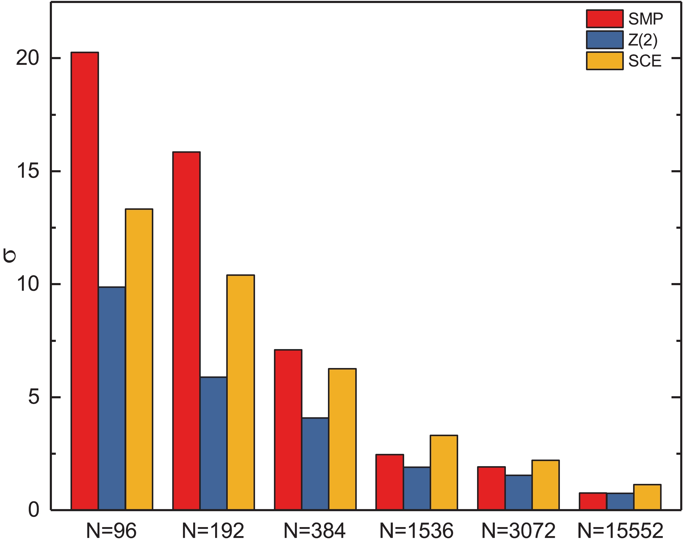
Figure A1.
(color online) $\sigma$ of${\rm{Tr}}\left(\gamma_{3}M^{-1}\right)$ as a function of the number of source vectors N.
Figure A2. (color online) Method error of
${\rm{Tr}}\left(\gamma_{5}\gamma_{1}M^{-1}\right)$ as a function of the number of source vectors N.
Figure A3. (color online) Method error of
${\rm{Tr}}\left(\sigma_{34}M^{-1}\right)$ as a function of the number of source vectors N.$\Gamma$ 

method $N=96$ 

$N=192$ 

$N=384$ 

$N=1536$ 

$N=3072$ 

$N=15552$ 

$\gamma_{3}$ 

SMP 205.18% 269.00% 174.39% 129.72% 123.95% 101.65% SCE 134.94% 176.29% 153.68% 174.92% 142.95% 154.08% $\gamma_{5}\gamma_{1}$ 

SMP 66.81% 63.66% 55.92% 37.60% 52.31% 47.30% SCE 43.32% 52.49% 46.56% 41.89% 57.33% 48.15% $\sigma_{34}$ 

SMP 72.78% 54.20% 47.71% 64.61% 70.62% 73.00% SCE 84.09% 60.01% 79.27% 87.96% 90.24% 133.93% Table A1.
$\sigma /\sigma_{Z\left(2\right)}$ for the SMP and SCE methods for different N.
Calculation of disconnected quark loops in lattice QCD
- Received Date: 2019-11-22
- Available Online: 2020-03-01
Abstract: Calculation of disconnected quark loops in lattice QCD is very time consuming. Stochastic noise methods are generally used to estimate these loops. However, stochastic estimation gives large errors in the calculations of disconnected diagrams. We use the symmetric multi-probing source (SMP) method to estimate the disconnected quark loops, and compare the results with the


 DownLoad: