


 Abstract
 HTML
HTML Reference
 Related
 PDF
PDF


-
In astrophysics and cosmology, the accretion of fluids or matter onto massive objects, such as black holes (BHs) or stars, is an interesting physical phenomenon. Accretion plays an important role in constraining the astronomical observation, and it can not only increase the mass of a BH, but also its angular momentum. Accretion is defined as the process by which massive astrophysical objects such as stars and BHs capture matter from their surroundings, which leads to an increase/decrease in mass and angular momentum. During the evolutionary phases of dusty plasma clouds, planets and stars are formed as a result of the accretion process. The existence of supermassive BHs at galaxy centers suggests that they could have formed via the accretion process. The accretion of phantom energy shows that the mass of a BH not always increases, but also could decrease [1, 2]. In 1952, Bondi investigated the accretion process for a star within the Newtonian framework [3]. After evolution of the relativistic theory of gravitation by Einstein, astrophysicists could study the accretion process within the relativistic framework. Michel was the first to investigate the accretion process onto the Schwarzschild BH [4]. Further, Shapiro and Teukolsky [5] also contributed to Michel's idea. Later on, Babichev et al. [6] discussed the effect of accretion of dark energy onto the Schwarzschild BH and found that the accretion of phantom energy decreases the mass of the BH. Debnath [7] further generalized Babichev's concept and proposed a system of accretion onto general static spherically symmetric BHs. Accretion onto charged BHs in the Einstein and massive theories of gravity is discussed in Ref. [8]. The effects of Lorentz breaking on the accretion onto the Schwarzschild BH were analyzed by Ref. [9]. The thin accretion disk around a rotating Kerr-like BH in the Einstein-bumblebee gravity model was examined in Ref. [10]. Spherically-symmetric accretion onto a black hole at the Center of a Young Stellar Cluster was investigated by Ref. [11]. Moreover, in a series of recent papers [12–18], the accretion of spherically symmetric spacetime was investigated. The authors were mainly interested to determine how the presence of cosmological constants affects the accretion rate.
After the first discovery of gravitational waves (GW) on September 14th, 2015 (GW150914) [19], the Laser Interferometer Gravitational wave Observatory (LIGO) detected GWs for the third time on January 4th, 2017 (GW170104) [20]. This provides clear evidence for the presence of BHs and assures that BHs are the common objects in the universe. The behaviour of BHs will be observed at large in the near future. The detection of GWs opens new doors for research in general relativity [21] and cosmology. Several theories are employed to test alternative theories of gravity, where the Lorentz invariance (LI) is broken, which influences the scattering connection for GW [20]. For the first time, these theories utilized (GW170104) to assume maximum magnitudes of the Lorentz infringement, authorized by their information to some extent. The limits were revealed to be critical.
The Einstein-aether theory was originally proposed as a system for breaking the local Lorentz symmetry, while maintaining as many characteristics of general relativity as possible. The Einstein-Aether theory is essentially general relativity coupled to a time, like the unit vector field
$ v^a $ , which cannot disappear even in a local frame [22, 23]. The Einstein-aether theory is used as a strong argument of Lorentz symmetry that violates gravity. If spacetime continuity is reduced to a discrete structure, then the violation of Lorentz symmetry might occur at quantum gravity or Planck scales, making spacetime an emergent phenomenon. This proved to be very helpful in obtaining quantitative constraints on the Lorentz violating gravity [24]. Violations of the Lorentz symmetry in the gravitational sector were extensively employed to develop modified gravity theories that explain dark matter phenomenology without taking into account the existence of dark matter [22]. In the Einstein-aether theory, the background tensor fields break the Lorentz symmetry down to a rotation subgroup, as a result of the existence of a preferred time direction at every point in spacetime, i.e., existence of a preferred frame of reference established by the aether vector field$ v^a $ . The introduction of the aether vector field permits several novel effects, e.g., matter fields that can travel faster than the speed of light [25] and dubbed superluminal particles [26]. Furthermore, Horava proposed that better ultra-violet properties can be achieved by giving up Lorentz symmetry [24]. Barausse and Sotiriou presented a no-go theorem for slowly rotating BHs in the Horava-Lifshitz gravity [27]. Later on, they modified this claim by introducing a relation between the Horava-Lifshitz gravity and Einstein-aether theory [28]. Slowly rotating BHs in the Einstein-aether theory show that solutions that are free from naked finite area singularities form a two-parameter family, i.e., mass and angular-momentum of BH, whereas there is no independent aether charge [22]. Recently, Zhu et al. [29] discussed the shadow and deflection angle of two kinds of charged and slowly rotating BHs in Einstein-aether theory.The aim of this study is to examine matter accretion of different fluids onto Einstein-aether BHs with several astrophysical and cosmology signatures. One approach to observe the differences among different BHs is the study of the accretion process. Generally, most astrophysical objects grow substantially in mass due to accretion. The most important information on astrophysical objects is obtained from the observation of the gas stream motion in the gravitational field of compact objects. The presence of a mass accretion rate of astrophysical objects provides strong evidence for the existence of a surface of compact objects like BHs and stars. Therefore, the study of the mass accretion rate is a powerful indicator of their physical nature. The basic aim of the present study is to investigate the matter accretion rate of first and second kind Einstein-aether BHs. Particular signatures can appear in ultra-stiff, ultra-relativistic, radiation, and sub-relativistic fluids, which enables direct testing of different models of Einstein-aether BHs. By discussing the effects of the first and second kind Einstein-aether BHs, we found that the consequences of matter accretion in the case of Einstein-aether BHs are more significant, and metrics of the Einstein-Aether BHs are more realistic in comparison to others in the literature.
In this study, we concentrate on the accretion of perfect fluids onto the first and second kind Einstein-aether BHs by adopting the Hamiltonian approach [30, 31]. The remainder of the paper is organized as follows: in Section 2, we discuss the metric function of first and second kind Einstein-aether BHs. In Section 3, we discuss the method to derive conservation laws for the accretion process, expression for the speed of sound at the sonic (critical) point, and also discuss the general formulism. In Section 4, we address the dynamical framework of the Hamiltonian with the equation of state (EoS) for the accretion process of isothermal fluids. We also observe the behavior of fluid flow around the first and second kind Einstein-aether BHs for different kind of fluids, such as ultra-relativistic fluid
$ (k = 1/2) $ , ultra-stiff fluid$ (k = 1) $ , sub-relativistic fluid$ (k = 1/4) $ , radiation fluid$ (k = 1/3) $ . In Section 5, we discuss general solutions of polytropic EoS and apply our Hamiltonian dynamical analysis results to polytropic fluid. In Section 6, we calculated the mass accretion rate for first and second kind Einstein-aether BHs in the presence of different fluids. The final section of this paper presents the conclusion and discussions of the above derivations and results. We employ the basic relativistic notation, and the metric mark is (−,+,+,+) in this paper. -
The general Einstein-aether action theory is developed employing two assumptions.
● It is a general covariant advancement of general relativity.
● It is a functional of spacetime metric
$ g_{ab} $ and a timelike unit vector field$ v^a $ , which involves second order derivatives, such that the final field equations consist of a double derivative of$ g_{ab} $ ,$ v^a $ , and the higher derivative is zero.Then, the Einstein-Aether action theory is described by [26],
$ S = \int {\rm d}^4x\sqrt{-g}\left [\frac{1}{16 \pi G_{{\text{æ}}}}(\Re+{\text{Ł}}_{{{\text{æ}}}}) \right], $

(1) where
$ G_{{\text{æ}}} $ is the constant of gravitational aether, and$ {\text{Ł}}_{{{\text{æ}}}} $ is the aether lagrangian$ -{\text{Ł}}_{{{\text{æ}}}} = Z^{ab}_{cd}(\nabla_a v^c)(\nabla_b v^d) - \lambda(v^2+1), $

(2) with
$ Z^{ab}_{cd} = b_1 g^{ab}g_{cd}+b_2 \delta^a_c \delta^b_d + b_3 \delta^a_d \delta^b_c - b_4 v^a v^b g_{ab}, $

(3) where coupling constants of the Einstein-aether theory are represented by
$ b_i $ $ (i = 1,2,3,4) $ . There are numerous hypothetical and observational limits on coupling constants$ b_i $ [32-34]. For sufficiently large coupling conditions, Einstein-aether terms can dominate the general relativity terms [33]. Oost et al. found that the events of$ {\rm GRB}170817 $ and$ {\rm GW}170817 $ imply extreme conditions, where$ |b_{13}|<10^{-19} $ a. Here, we do not address these extreme conditions and focus on the violation of Lorentz gravity theory [35]. We apply the conditions$ 0\leqslant b_{14} <2 ,\; \; \; 2 + b_{13} + 3 b_2 > 0, \; \; \; 0\leqslant b_{13} <1, $

(4) where
$ b_{14} \equiv b_1 + b_4 $ and$ b_{13} \equiv b_1 + b_3 $ . The line element of a spherically symmetric metric can be written as$ {\rm d}s^2 = - Y(r) {\rm d}t^2 + \frac{{\rm d}r^2}{Y(r)} + r^2({\rm d}\theta^2 + {\rm sin}^2\theta {\rm d}\phi^2). $

(5) Two types of exact solutions exist for Einstein-aether BHs [36, 37]. The metric function
$ Y(r) $ for the first kind Einstein-aether BH$ (b_{14} = 0, b_{123}\neq 0) $ is written as$ Y(r) = 1 - \frac{2M}{r} - \frac{27 b_{13}}{256(1-b_{13})} \bigg(\frac{2M}{r}\bigg)^4. $

(6) If
$ b_{13} = 0 $ , we obtain a Schwarzschild BH. The Killing horizon is located on$ Y(r) = 0 $ , that is [37]$ r_{KH} = M\left(\frac{1}{2}+\alpha+\sqrt{\gamma-\beta+ \frac{1}{4\alpha}}\right), $

(7) where
$ \begin{split}\alpha = & \sqrt{\frac{1}{4}+\beta},\; \; \; \; \beta = \frac{2^{\textstyle\frac{7}{3}} \epsilon}{\gamma}+\frac{\gamma}{3\cdot2^{\textstyle\frac{1}{3}}},\; \\ \gamma = & (27\epsilon+3\sqrt{3}\epsilon\sqrt{27-256\epsilon})^{1/3}, \epsilon = \frac{27 b_{13}}{256(1-b_{13})}. \\ \end{split}$

(8) The metric function
$ Y(r) $ for the second kind Einstein-aether BH$ (b_{14}\neq0, b_{123} = 0) $ is written as$ Y(r) = 1 - \frac{2M}{r} - \frac{b_{13}-\dfrac{b_{14}}{2}}{(1-b_{13})} \left(\frac{M}{r}\right)^2 , $

(9) and the roots of
$ Y(r) = 0 $ are$ r_{KH} = M\left(1+ \sqrt{\frac{1-\dfrac{b_{14}}{2}}{1-b_{13}}}\right), $

(10) $ r_{UH} = M\left(1- \sqrt{\frac{1-\dfrac{b_{14}}{2}}{1-b_{13}}}\right). $

(11) If
$ b_{13} = b_{14}/2 $ , this becomes a Schwarzschild BH. For$ b_{14}\leqslant 2b_{13} $ , the mass of the Einstein-aether BH$M_{ae} = $ $ -b_{14}\dfrac{M_{ADM}}{2} $ is contributed to by the aether field, where$ M_{ADM} $ is the Komar mass [37]. There is a universal horizon hiding behind the Killing horizon. The universal horizon can capture particles moving with an arbitrary velocity i.e., super-luminal particles, while Killing horizons are unable to capture these particles. The universal horizon has no effect on radiating luminal or subluminal particles during the Hawking radiation [38]. In the following section, we discuss the accretion process on Einstein-aether BHs for the coupling constants$ b_{13} = 0.4, 0.6, 0.8 $ and$ b_{14} = 0.2 $ as observational constraints presented in Refs. [26, 39]. -
We employ the notation for thermodynamic functions of the fluid as the Hamiltonian H, temperature T, energy density
$ \rho $ , specific enthalpy h, specific entropy s, pressure p, baryon number density n, and the four-velocity vector$ u^\mu $ . Here,$ a^2 = \left(\dfrac{\partial p }{\partial \rho}\right)_s $ , where a is the 3-D speed of sound in the locally inertial frame. When the entropy s is constant, this leads to$ a^2 = \dfrac{{\rm d}p}{{\rm d}\rho} $ , which is the case of static spherically symmetric BHs accretion by a perfect fluid. Employing the line element (5), it is easy to demonstrate Eqs. (5), (7), (10), (15), (17), (19), (20), and (21) of Ref. [30]$ u_t = \pm \sqrt{Y(r)+ u^2}, \; \; \; r^2 n u = E_1 \neq 0, $

(12) $ h\sqrt{Y(r)+ u^2} = E_2, \; \; \; v^2 = \frac{u^2}{Y(r)+u^2}, $

(13) $ u^2 = \frac{Y(r) v^2}{1-v^2} , \; \; \; E_1^2 = \frac{r^4 n^2 Y(r) v^2}{1-v^2}, $

(14) $ G(n) \equiv nF'(n)-F(n) , \; \; \; a^2 \equiv n ({\rm ln}F')', $

(15) where
$ (E_1,E_2) $ are constants of integration;$ u = u^r $ ;$ F(n) \equiv e $ ; e is the simple canonical form of the EoS; v is the three-velocity of fluid, whose value lies in the interval$ (-1,1) $ for a locally inertial frame. The second part of Eq. (14) is obtained by the law of particle conservation,$ \bigtriangledown_\mu (nu^\mu) = 0, $ and$ hu_\mu \chi^{\alpha\beta}, \; [ \chi^{\alpha\beta} = (1,0,0,0) $ , which is referred to as the timelike Killing vector] [40]. This constant value is the inertial-equivalent generalization of the energy conservation equation$ mu_\mu \chi^{\alpha\beta} $ .The constant
$ E_1^2 $ in Eq. (14) can be written as$ \dfrac{r^4 n_0^2 Y_0 v_0^2}{1-v_0^2} $ , where$ 0 $ denotes any reference point$ (r_0,v_0) $ from the phase representation, which could be a critical point. If spatial infinity$ r_\infty $ and$ v_\infty $ , or any other reference point exists, we obtain$ \frac{n^2}{n_0^2} = \frac{Y_0 r_0^2 v_0^2}{1-v_0^2} \frac{1-v^2}{Y r^4 v^2} = E_1^2 \frac{1-v^2}{Y r^4 v^2}. $

(16) From this equation, it is clear that the value of specific enthalpy h depends only on
$ (Y(r), r^2) $ . This means that only the metric components$ Y(r) $ and$ r^2 $ define the dynamic system via the Hamiltonian. We thus reach the conclusion that the perfect fluid accretion onto different static spherically symmetric BHs would be the same if these BHs had the same functions$ (Y(r),r^2) $ [40].The case
$ E_1 = 0 $ , both scenarios of$ n = 0 $ in Eq. (12), indicating no fluid, or$ v = 0 $ in Eq. (14) and any n, indicating no flow, is not useful. Thus, we consider$ E_1 \neq 0 $ . Because the fluid cumulates near the Killing horizon$ (r \rightarrow r_{KH}) $ ,$ Y(r)\rightarrow 0 $ , the following two cases may be considered in Eq. (16)1. v approaches
$ \pm 1 $ , and n has two possibilities, the first being convergent and second divergent for$ (r \rightarrow r_{KH}) $ .2. v approaches zero, and n does not converge in this case. The fluid approaches the Killing horizon that causes pressure divergence, resulting in the fluid repulsion in reverse.
The law of particle conservation (14) holds for all non-perfect fluids, even in the case where that fluid contains a single particle species. This is valid for real fluids as well.
The dynamical Hamiltonian system
$ (H) $ corresponds to$ E_1^2 $ (14) in constant motion. Employing Eqs. (13) and (14), we obtain$ H(r,v) = \frac{h(r,v) Y(r)}{1-v^2}. $

(17) For the derivation of the sonic point, the dynamical system of the Hamiltonian H given in Eq. (17) reads as [41, 42]
$ \dot{r} = H,_v \; ,\; \; \; \dot{v} = -H,_r\; , $

(18) where
$ \dot{r} = \frac{{\rm d}r}{{\rm d}t} \; ,\; \; \; \dot{v} = \frac{{\rm d}v}{{\rm d}t}. $

(19) For Eq. (18), in the partial differentiation of
$ \dfrac{\partial H}{\partial v} $ and$ \dfrac{\partial H}{\partial r} $ , where r and v are treated as constants, respectively. We obtain the following result$ \dot{v} = - \frac{h^2}{1-v^2} \left(r \left(\frac{{\rm d}}{{\rm d}r}Y(r) \right)(1-a^2)-4 a^2 Y(r) \right), $

(20) $ \dot{r} = \frac{2 h^2 Y(r)}{v(1-v^2)}(v^2-a^2). $

(21) By letting Eqs. (20) and (21) equal to zero, we obtain the critical points as follows:
$ v_c^2 = a_c^2 \; , \; \; \; r_c (1-a_c^2) \frac{{\rm d}}{{\rm d}r_c}Y(r_c) = 4 a_c^2 Y(r_c). $

(22) The above equation represents the speed of sound at critical points
$ a_c^2 $ in terms of$ r_c $ . After simplification of the second part of Eq. (22), we obtain$ a_c^2 = \frac{r_c \dfrac{{\rm d}}{{\rm d}r_c}Y(r_c)}{4 Y(r_c)+r_c \dfrac{{\rm d}}{{\rm d}r_c}Y(r_c)}, $

(23) The three-dimensional speed of sound at critical points is represented by
$ a_c $ . The first part of Eq. (22) expresses the three-velocity of the fluid equivalent to the speed of sound at critical points. -
The fluid flow at constant temperature is referred to as isothermal fluid. When the fluid flows with the speed of light, it does not release or absorb energy from its neighborhood. Therefore, our dynamical system shifts to an adiabatic system. The EoS for this type of fluid is of the form
$ p = k \rho $ , where k is a state parameter. Generally, the speed of sound at constant temperature is$ a^2 = \frac{{\rm d}p}{{\rm d}\rho} $ , which leads to$ a^2 = k $ . According to the first law of thermodynamics$ \frac{{\rm d}\rho}{{\rm d}n} = \frac{\rho+p}{n} = h, $

(24) by integrating the above equation, we find
$ n = n_c \left(\frac{\rho}{\rho_c}\right)^{\textstyle{(\frac{1}{k+1})}}, $

(25) and comparing the above equation to enthalpy, we obtain
$ h = \frac{(k+1)\rho_c}{n_c} \Big(\frac{n}{n_c}\Big)^k. $

(26) Inserting Eq. (26) in Eq. (13) yields
$ n^k \sqrt{Y(r)+(u)^2} = E_2, $

(27) where
$ E_2 = \dfrac{E_1 n_c^{1-k}}{(k+1)\rho_c} $ . By comparing the second part of Eq. (12) and Eq. (27), we obtain$ \sqrt{Y(r)+(u)^2} = E_3 r^k (u)^k . $

(28) Here, the Hamiltonian is defined as
$ H = \frac{Y(r)^{1-k}}{(1-v^2)^{1-k}v^{2k}r^{2k}}. $

(29) It is interesting to discuss the behavior of fluid at the critical point. We analyzed the behavior of different kinds of fluids, such as ultra-relativistic fluid (
$ k = 1/2 $ ), sub-relativistic fluid ($ k = 1/4 $ ), radiation fluid ($ k = 1/3 $ ), and ultra-stiff fluid ($ k = 1 $ ). These fluids are discussed in the following subsections. -
When the energy density is equal to the isotropic pressure, then this particular fluid is referred to as ultra-stiff fluid i.e.,
$ p = \rho $ . The Hamiltonian (29) assumes the form$ H = \frac{1}{v^2r^4}. $

(30) We plot the velocity of the ultra-stiff fluid v with respect to r in Fig. 1, and the trajectories exhibit two kinds of fluid motion, namely
$ (1) $ subsonic accretion flow in the lower region$ (v<0) $ and$ (2) $ supersonic accretion flow in the upper region$ (v>0) $ . The critical point for the first kind Einstein-aether BH shifts towards singularity, as compared to the second kind Einstein-aether BH.
Figure 1. (color online) Behavior of Hamiltonian (30) for first kind Einstein-aether BH with
$M=1, b_{13}=0.6$ (left panel). Parameters are$r_c\approx2.228665389, v_c = 1 ~~ H_c\approx0.04053409918$ . Behavior of Hamiltonian (30) for second kind Einstein-aether BH with$M=1, b_{13}=0.6, b_{14}=0.2 $ (right panel). Parameters are$r_c\approx2.5, v_c=1, ~H_c\approx0.0256$ . -
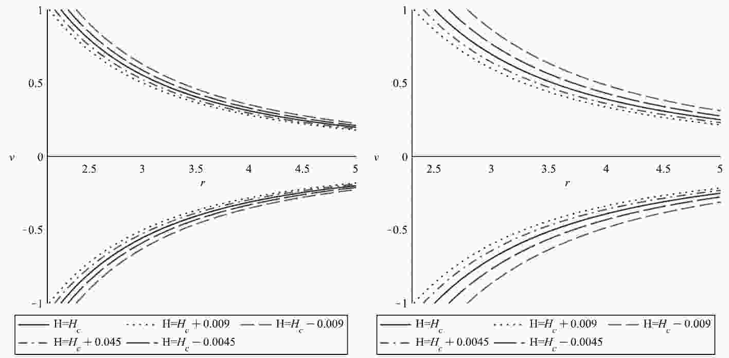
For ultra relativistic fluids, we consider EoS
$ p = \frac{\rho}{2} $ , which indicates that the pressure of fluid is half the matter density. The Hamiltonian (29) reduces the form for the first and second kind Einstein-aether BHs, respectively as:$ H = \frac{\sqrt{1 - \dfrac{2M}{r} - \dfrac{27 b_{13}}{256(1-b_{13})}\Big(\dfrac{2M}{r}\Big)^4 }}{r^2v \sqrt{(1-v^2)}}. $

(31) $ H = \frac{\sqrt{1 - \dfrac{2M}{r} - \dfrac{b_{13}-\dfrac{b_{14}}{2}}{1-b_{13}}\Big(\dfrac{M}{r}\Big)^2}}{r^2v \sqrt{(1-v^2)}}. $

(32) We plot the velocity of the ultra-relativistic fluid v with respect to r in Fig. 2. The trajectory of the fluid describes the following four types of fluid.
$ (1) $ Subsonic accretion followed by supersonic accretion (lower plot) and supersonic out flow followed by subsonic motion (upper plot).$ (2) $ Purely supersonic accretion for$ v<-v_c $ and purely supersonic outflow for$ v>-v_c $ .$ (3) $ Subsonic flow out followed by subsonic accretion for$ v_c>v>-v_c $ .$ (4) $ Subsonic and supersonic accretion appears in the range$ -v_c<v<0 $ and$ -1<v<-v_c $ , while the subsonic/supersonic flows in the range$ 1>v>v_c $ ,$ 0<v<v_c $ , respectively. We analyze this supersonic accretion followed by subsonic accretion and ending inside the Killing horizon. This does not provide support to claim that the flow must be supersonic at the Killing horizon. The fluid outflow is assumed to start at the Killing horizon because of its high pressure, which prompts divergence. The fluid under the effects of its own pressure flows back to spatial infinity. Thus, the flow of the fluid is neither transonic nor supersonic near the Killing horizon. The critical point shifted towards singularity for the first kind Einstein-aether BH as compared to second kind Einstein-aether BH. The value of the Hamiltonian at the critical point is lower for the second kind Einstein-aether BH than for the first kind. In dynamical systems, these new solutions are related to instability and fine-tuning issues. The issue of stability is related to the nature of saddle points (critical points$ (r_c,v_c) $ and$ (r_c,-v_c) $ ) of the Hamiltonian function. This outflow is unstable, as it follows a subsonic path passing through the saddle point$ (r_c,v_c) $ and becomes supersonic with a speed nearly equal to the speed of light. The solution curve converges and diverges, which indicates that the point$ (r = r_{KH},v = 0) $ is seen as an attractor as well as a repeller, respectively, for the cosmological purpose.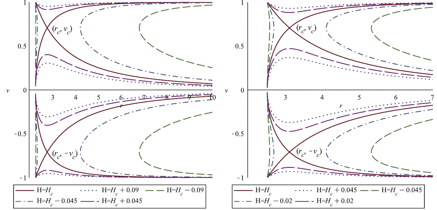
Figure 2. (color online) Behavior of Hamiltonian (31) for first kind Einstein-aether BH with
$M=1, b_{13}=0.6$ . The parameters are$r_c\approx2.744809564, v_c\approx0.7071067810~~ ,H_c\approx0.1264113037$ . Behavior of Hamiltonian in Eq. (32) for second kind Einstein-aether BH with$M=1, b_{13}=0.6, b_{14}=0.2$ (right panel). Parameters are$r_c\approx3.104049622, v_c\approx0.7071067810, ~~ H_c\approx0.09866786226$ . -
The fluid obeying the EoS in the form
$ p = \dfrac{\rho}{3} $ and absorbing the radiation emitted by BH is referred to as radiation fluid. The Hamiltonian (29) extracts the simple form for the first and second kind Einstein-aether BHs, respectively:$ H = \frac{\left(1 - \dfrac{2M}{r} - \dfrac{27 b_{13}}{256(1-b_{13})}\left(\dfrac{2M}{r}\right)^4 \right)^{\textstyle\frac{2}{3}}}{r^{\textstyle\frac{4}{3}}v^{\textstyle\frac{2}{3}}(1-v^2)^{\textstyle\frac{2}{3}}}. $

(33) $ H = \frac{\left(1 - \dfrac{2M}{r} - \dfrac{b_{13}-\dfrac{b_{14}}{2}}{1-b_{13}}\left(\frac{M}{r}\right)^2\right)^{\textstyle\frac{2}{3}}}{r^{\textstyle\frac{4}{3}}v^{\textstyle\frac{2}{3}}(1-v^2)^{\textstyle\frac{2}{3}}}. $

(34) We plot the velocity of radiation fluid v with respect to r in Fig. 3. The radiation fluid exhibits subsonic flow in the range
$ 0<v<v_c $ and supersonic flow in the range$ v_c<v<1 $ . It furthermore exhibits similar behavior to ultra-relativistic fluids for$ v>0 $ and unphysical behavior for$ v<0 $ . Our analysis shows that the critical point shifted towards singularity for the first kind Einstein-aether BH as compared to the second kind.
Figure 3. (color online) Behavior of Hamiltonian (33) for first kind Einstein-aether BH with
$M=1, b_{13}=0.6$ (left panel). Parameters are$r_c\approx3.226152597, v_c\approx0.5773502693~~ ,H_c\approx0.1993991936 $ . Behavior of Hamiltonian in Eq. (34) for second kind Einstein-aether BH with$M=1, b_{13}=0.6, b_{14}=0.2$ (right panel). Parameters are$r_c\approx3.679449472, v_c\approx0.5773502693,~~ H_c\approx0.1696469105$ . -
The fluid obeying the EoS in the form
$ p = \frac{\rho}{4} $ is referred to as sub-relativistic fluid. The isotropic pressure is one fourth of the energy density. The Hamiltonian (29) reduces the simplest form for the first and second kind Einstein-aether BHs, respectively, as follows$ H = \frac{\left(1 - \dfrac{2M}{r} - \dfrac{27 b_{13}}{256(1-b_{13})}\left(\dfrac{2M}{r}\right)^4 \right)^{\textstyle\frac{3}{4}}}{rv^{\textstyle\frac{1}{2}}\big(1-v^2\big)^{\textstyle\frac{3}{4}}}. $

(35) $ H = \dfrac{\left(1 - \dfrac{2M}{r} - \dfrac{b_{13}-\dfrac{b_{14}}{2}}{1-b_{13}}\left(\dfrac{M}{r}\right)^2\right)^{\textstyle\frac{3}{4}}}{rv^{\textstyle\frac{1}{2}}\big(1-v^2\big)^{\textstyle\frac{3}{4}}}. $

(36) We plot the velocity of the sub-relativistic fluid v with respect to r in Fig. 4 and compare the fluid flow behavior for the first and second kind Einstein-aether BHs. The sub-relativistic fluid exhibits subsonic flow in the range
$ 0<v<v_c $ and supersonic flow in the range$ v_c<v<1 $ . Supersonic outflow is followed by subsonic motion for$ v>0 $ . Furthermore, sub-relativistic fluid exhibits a similar behavior to ultra-relativistic fluid for$ v>0 $ . The critical point shifts towards singularity for the first kind Einstein-aether BH as compared to the second kind Einstein-aether BH.
Figure 4. (color online) Behavior of Hamiltonian (35) for first kind Einstein-aether BH with
$M=1, b_{13}=0.6$ (left panel). Parameters are$r_c\approx3.699904864, v_c=0.5, H_c\approx0.2588120232$ . Behavior of Hamiltonian (36) for second kind Einstein-aether BH with$M=1, b_{13}=0.6, b_{14}=0.2$ (right panel). Parameters are$r_c\approx4.237468593, v_c\approx0.5,~~ H_c\approx0.2307014368$ .We investigated non-transonic solutions in the above cases. However, it is also important to discuss the flows that pass through the transonic point. The maximum accretion rate obtained by spherical accretion is known as transonic flow. The behavior of transonic flow for the above-mentioned fluids is shown in Figs. 5 and 6. From Fig. 5 shows that the transonic solution does not form a close orbit, such that it is not possible to obtain homoclinic orbits around the first kind Einstein-aether BH and Schwarzschild BH in the case of subsonic solutions. In the absence of coupling constants (aether parameters), we obtain a non-homoclinic orbit, as shown in right panel of Fig. 5. Furthermore, we observe the following key points
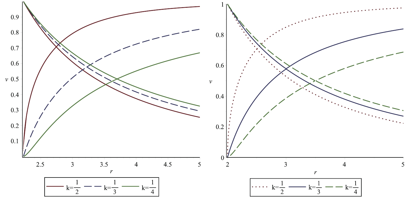
Figure 5. (color online) Behavior of transonic solution of first kind Einstein-aether BH for
$M=1, b_{13}=0.6$ (left panel). Behavior of transonic solution of Schwarzschild BH (right panel).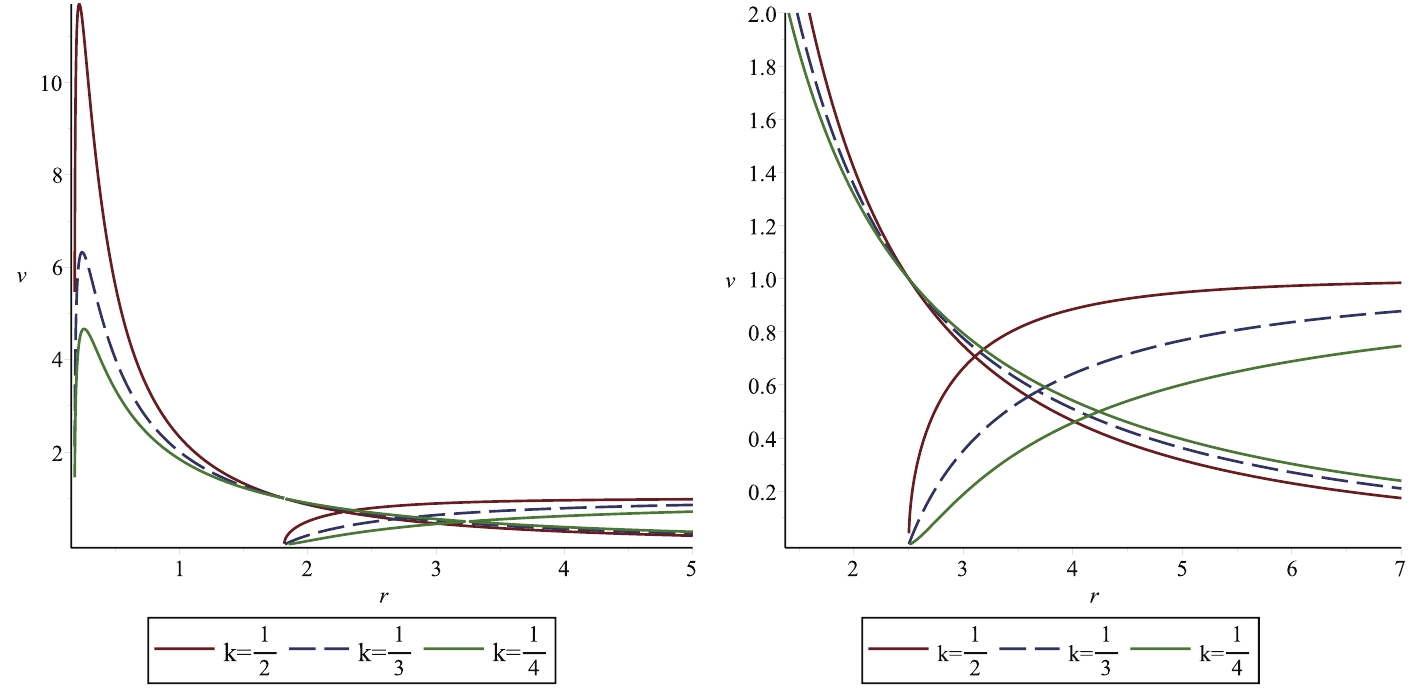
Figure 6. (color online) Homoclinic orbits of transonic solution for
$M=1, b_{13}=0.2$ and$b_{14}=1.2$ (left panel), and non-homoclinic orbits of transonic solution for$M=1, b_{13}=0.6$ and$b_{14}=0.2$ (right panel) of second kind Einstein-aether BH.● For an ultra-relativistic fluid,
$ r_c\approx2.744 $ for the first kind Einstein-aether BH and$ r_c\approx 2.499 $ for a Schwarzschild BH.● For a radiation fluid,
$ r_c\approx3.225 $ for the first kind Einstein-aether BH and$ r_c\approx 2.999 $ for a Schwarzschild BH.● For a sub-relativistic fluid,
$ r_c\approx 3.698 $ for the first kind Einstein-aether BH and$ r_c\approx 3.501 $ for a Schwarzschild BH.From the above analysis, we conclude that the critical radius approaches singularity for the aforementioned fluids in Schwarzschild BH, as compared to the first kind Einstein-aether BH. We noted some important findings; i.e., from the left panel of Fig. 6, we observe the closed orbit in the transonic solution, which leads to the possibility to find the homoclinic orbit in the case of the subsonic solution. From the right panel of Fig. 6, we do not find the closed orbit, which represents the non-homoclinic orbit in the case of a subsonic solution for the given condition
$ b_{14}<2b_{13} $ ,$ b_{13}, b_{14}\neq 0 $ . Moreover, we observe two important cases in the left panel of Fig. 6● For
$ r>1.8 $ , we obtain the transonic solution.● For
$ r<1.8 $ , we observe the homoclinic orbits with superluminal motion as$ v>1 $ in the second kind Einstein-aether BH for higher values of$ b_{14} $ .In the right panel of Fig. 6, we find
● For
$ r>2.5 $ , we obtain a transonic solution.● For
$ r<2.5 $ , we note non-homoclinic orbits with superluminal motion as$ v>1 $ in the second kind Einstein-aether BH for lower values of$ b_{14} $ . -
The polytropic EoS is given in Ref. [30]
$ p \equiv G(n) \equiv \eta n^\gamma, $

(37) where
$ \eta $ ,$ \gamma $ are arbitrary constants, and$ \gamma $ is positive for ordinary matter. From the first part of Eq. (15) and Eq. (37), we derive the relation of the specific enthalpy h [30].$ h = m+\frac{k\gamma n^{\gamma-1}}{\gamma-1}, $

(38) where the baryonic mass is expressed by m. By Eq. (38) and the second part of Eq. (15), we have
$ a^2 = \frac{(\gamma -1)\omega}{m(\gamma-1)+\omega}, $

(39) where
$ (\omega = \eta \gamma n^{\gamma -1}) $ $ h = m\frac{(\gamma -1)}{\gamma-1-a^2}. $

(40) Employing Eqs. (17) and (38), we have
$ h \equiv m \bigg(1+Q\bigg( \frac{1-v^2}{r^4 Y(r) v^2}\bigg)\bigg)^{\textstyle{\frac{\gamma-1}{2}}}, $

(41) where
$ Q \equiv\frac{\eta \gamma n_c^{\gamma-1}}{m(\gamma -1)}\Big(\frac{r_c^5 Y(r_c),r_c}{4}\Big)^{\textstyle{\frac{\gamma -1}{2}}} = {\rm constant}. $

(42) By plugging Eq. (41) in Eq. (17), we obtain the new form of the Hamiltonian system,
$ H = \frac{Y(r)}{1-v^2} \bigg(1+Q\bigg(\frac{1-v^2}{r^4 Y(r)v^2}\bigg)^{\textstyle{\frac{\gamma -1}{2}}}\bigg)^2. $

(43) ● Hamiltonian for the first kind Einstein-aether BH
$ \begin{split} H =& \frac{1 - \dfrac{2M}{r} - \dfrac{27 b_{13}}{256(1-b_{13})}\Big(\dfrac{2M}{r}\Big)^4}{1-v^2} \\ &\times\left(1+Q\left(\frac{1-v^2}{r^4v^2\Big(1 - \dfrac{2M}{r} - \dfrac{27b_{13}}{256(1-b_{13})}\Big(\dfrac{2M}{r}\Big)^4\Big)}\right)^{\textstyle{\frac{\gamma -1}{2}}}\right)^2.\end{split}$

(44) ● Hamiltonian for the second kind Einstein-aether BH
$ \begin{split}H =& \frac{1 - \dfrac{2M}{r} - \dfrac{b_{13}-\dfrac{b_{14}}{2}}{(1-b_{13})}\Big(\dfrac{M}{r}\Big)^2 }{1-v^2} \\ &\times\left(1+Q\left(\frac{1-v^2}{r^4v^2\Big(1 - \dfrac{2M}{r} - \dfrac{b_{13}-\dfrac{b_{14}}{2}}{(1-b_{13})}\Big(\dfrac{M}{r}\Big)^2 \Big)}\right)^{\textstyle{\frac{\gamma -1}{2}}}\right)^2. \end{split}$

(45) By analysis, we obtain that
$ \dfrac{{\rm d}Y(r)}{{\rm d}r} $ is positive for all r. Hence, the coefficient of$ \dfrac{Y(r)}{1-v^2} $ is positive because of the square in Eq. (43), while the coefficient$ \dfrac{Y(r)}{1-v^2} $ diverges as$ r \rightarrow \infty $ and the values of$ (1-v^2) $ lie in the interval$ (0,1) $ . Thus, the Hamiltonian diverges.Using the technique from Refs. [41, 42], we finally obtain the following expression
$ \left(\gamma -1-v_c^2\right)\left(\frac{1-v_c^2}{r_c^4 Y(r_c)v_c^2}\right)^{\textstyle{\frac{\gamma-1}{2}}} = \frac{n_c}{2Q}\left(r_c^5Y(r_c),r_c\right)^{\textstyle\frac{1}{2}}v_c^2, $

(46) $ v_c^2 = \frac{r_c Y(r_c),r_c}{r_cY(r_c),r_c+4Y(r_c)}. $

(47) Figure 7 shows the contour plot for the first (left panel) and second (right panel) kind Einstein-aether BH with
$ n_c = 0.19, Q = -\dfrac{1}{8}, \gamma = 0.5095 $ . We determine the new behavior of fluid by finding the precise critical points (sonic points)$ r_c \approx 2.809551576, v_c \approx 0.5421180342,\; H = H_c \simeq $ $ 0.3067992956 $ for the first kind Einstein-aether BH and vc≈0.2979550502, rc≈8.08065, H=Hc$\simeq $ 0.1946351870 for the second kind Einstein-aether BH. We find that the accretion for the first and second kind Einstein-aether BH initiates at subsonic flow as r approaches infinity, and subsequently follows supersonic flow avoiding the saddle (critical) point, ending at the Killing horizon. The supersonic outflow begins in the region of the Killing horizon avoiding the saddle (critical) point and ends subsonically as r approaches infinity. From Fig. 7 shows that the physical behavior of both BHs is different in the polytropic test fluid accretion, i.e., the trajectory for the first kind does not pass through the saddle point, while the trajectory for the second kind Einstein-aether BH passes through the saddle point.
Figure 7. (color online) Contour plot for first kind Einstein-aether BH with
$M=1, b_{13}=0.6$ (left panel). Contour plot for second kind Einstein-aether BH with$M=1, b_{13}=0.6$ and$b_{14} = 0.2$ (right panel).In Fig. 8, we consider
$ n_c = 0.001, \gamma = 1.5, Q = 0.125 $ for the first (left panel) and the second (right panel) kind Einstein-aether BH, which prompts four critical points. Three types of flow are discussed here,$ (i) $ non-relativistic outflow,$ (ii) $ subsonic non-global flow,$ (iii) $ non-heteroclinic flow, as solution curves avoid critical points, and accretion starts from the furthest left point and ends at the Killing horizon. Fig. 7 shows that the critical point is near singularity for the first kind Einstein-aether compared to the second kind Einstein-Aether BH. Other solutions could also be calculated at$ \gamma = 1.8 $ for the first kind Einstein-aether BH and at$ \gamma = \frac{5.5}{3} $ for the second kind Einstein-aether BH. Because the fluid is assumed as a test matter in the geometry of BHs, we examine the non-homoclinic shine, i.e., flow following a closed contour [41, 42].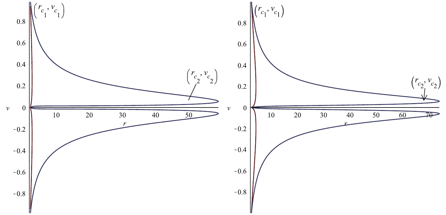
Figure 8. (color online) Contour plot for first kind Einstein-aether BH with
$M=1, b_{13}=0.6$ (left panel). Contour plot for second kind Einstein-aether BH with$M=1, b_{13}=0.6$ and$b_{14}=0.2$ . -
The rate of change in the mass of a BH is referred to as the mass accretion rate, and it is generally represented by
$\dot {\rm{M}}$ . It basically depicts the mass of the BH per unit time, which is defined as the area times flux of the BH at the Killing horizon. In this section, we discuss the effect of the radius on the accretion rate. The general expression to calculate it is$ \dot{M}|_{KH} = 4 \pi r^2 T_t^r |_{KH} $ [15], which refers to the relativistic statement of the flux of mass-energy density. For the perfect fluid, the energy-momentum tensor is given by$ T_t^r = (\rho+p)u_t u^r $ [41, 42]. The energy of our dynamical system is conserved, such that we have$ \nabla_\mu J^\mu \equiv 0 $ and$ \nabla_\nu T^{\mu\nu} \equiv 0 $ , given in Eqs. (12) and (13). From these conservation equations, we obtain$ r^2 u^r (\rho+p) \sqrt{(Y(r)+(u^r)^2)} = E_3, $

(48) where
$ E_3 $ is a constant of integration. Considering EoS$ p \equiv p(\rho) $ , the relativistic energy flux relation gives$ \frac{{\rm d}\rho}{\rho+p}+\frac{{\rm d}u^r}{u^r}+2\frac{{\rm d}r}{r} = 0. $

(49) By integrating the above equation, we have
$ r^2 u^r {\rm exp}\Big[\int_{\rho \infty}^\rho \frac{{\rm d}\acute{\rho}}{\acute{\rho}+p(\acute{\rho})}\Big] = -E_4, $

(50) where
$ E_4 $ is a constant of integration. The minus sign is assumed due to the negative value of$ u^r $ , and$ \rho_\infty $ is the density of matter at infinity. After simplification of Eqs. (50) and (48), we obtain$ E_5 = -\frac{E_3}{E_4} = (\rho+p)\sqrt{Y(r)+(u^r)^2} {\rm exp}\Big[-\int\frac{{\rm d}\acute{\rho}}{\acute{\rho}+p(\acute{\rho})}\Big] , $

(51) where
$ E_5 $ is a constant. Considering the boundary condition at infinity,$ E_5 \equiv \rho_\infty+p(\rho_\infty) = -\dfrac{E_3}{E_4} $ , here$ E_3 \equiv (\rho+ $ $p)u_t u^r r^2 = -E_4(\rho_\infty + p(\rho_\infty)) $ . If we divide Eq. (48) by the second part of Eq. (12), we obtain$ \frac{\rho+p}{n} \sqrt{Y(r)+(u^r)^2} = \frac{E_3}{E_1} \equiv E_7, $

(52) where
$ E_7 $ is a constant, such that$ E_7 = \frac{(\rho_\infty+p_\infty)}{n_\infty} $ . Using Eq. (48), we obtain the new relation of BH's accretion rate$ \dot{M} = -4 \pi r^2 u^r (\rho + p)\sqrt{Y(r)+(u^r)^2} = -4 \pi E_3, $

(53) then it becomes
$ \dot{M} = -4 \pi E_4(\rho_\infty+p(\rho_\infty)). $

(54) Because of the boundary condition at infinity, the above result holds for all fluids where EoS is valid in the form
$ p = p(\rho) $ . Hence, the BH accretion rate is defined as$ \dot{M} = -4 \pi E_4(\rho+p)|_{r = r_{KH}}, $

(55) at BH horizon
$ r_{KH} $ . Thus, evaluating Eq. (55) at$ r_{KH} $ , we obtain the mass accretion rate at the BH Killing horizon.We assume an isothermal EoS, i.e.,
$ p = k \rho $ , which implies that$ (\rho + p) \equiv \rho (1+k) $ . Then, Eq. (50) reduces to$ r^2 u^r \rho^{\frac{1}{1+k}} = - E_4 $ , that is$ \rho = \Big[-\frac{E_4}{r^2 u^r}\Big]^{1+k} , $

(56) with this expression of
$ \rho $ , Eq. (48) takes the form$ (u^r)^2 - \frac{E_3^2 E_4^{-2(1+k)}}{(1+k)^2} r^{4k} (-u^r)^{2k} + Y(r) = 0, $

(57) where
$ u^r $ can be obtained for given values of k. Using$ u^r $ , the energy density$ \rho(r) $ is obtained from Eq. (56). -
The radial component of the four-velocity by assuming
$ k = 1 $ in Eq. (57), is$ u^r = \pm 2E_4 \sqrt{\frac{Y(r)}{E_3^2 r^4- 4E_4^4}} . $

(58) The energy density is given by
$ \rho = \frac{(E_3^2 r^4-4E_4^4)}{4 E_4^2 r^4 Y(r)}. $

(59) Employing Eqs. (59) and (55), we obtain the mass accretion rate
$ \dot{M} = \frac{2 \pi (E_3^2 r^4-4E_4^4)}{E_4 r^4 Y(r)}. $

(60) 1. Mass accretion rate for first kind Einstein-aether BH
$ \dot{M} = \frac{2 \pi (E_3^2 r^4-4 E_4^4)}{E_4 \left(r^4 - 2 M r^3 - \dfrac{432 b_{13} M^4}{256(1-b_{13})}\right)}. $

(61) 2. Mass accretion rate for second kind Einstein-aether BH
$ \dot{M} = \frac{4\pi(E_3^2 r^4-4 E_4^4)(b_{13}-1)}{E_4 r^2 (2M^2b_{13}-M^2b_{14}- 4Mb_{13}r+2b_{13}r^2+4Mr-2r^2)}. $

(62) In Fig. 9, we plot the mass accretion rate for the first kind (left panel) and second kind (right panel) Einstein-aether BHs for the above-mentioned fluid. In the left panel, we observe that the mass accretion rate depends on the constants
$ (b_{13}) $ i.e., by increasing the constant value, the mass accretion rate is also increased. We note that the maximum accretion rate occurs near$ r\simeq 4.344, $ $4.231, 4.164, 3.436 $ for$ b_{13} = 0, 0.3, 0.6, 0.9 $ respectively. In the right panel, we find the maximum accretion rate for different values of coupling constants
Figure 9. (color online) Contour plot of mass accretion rate for first kind (left panel) Einstein-aether BH with
$M=1, E_3=-1, E_4=2$ and second kind (right panel) Einstein-aether BH with$M=1, E_3=1.5, E_4=2.85$ .●
$ b_{13} = 0, b_{14} = 0 $ , we have$ r\approx 5.356 $ .●
$ b_{13} = 0.4, b_{14} = 0.2 $ , we have$ r\approx 5.276 $ .●
$ b_{13} = 0.6, b_{14} = 0.2 $ , we have$ r\approx 5.063 $ .●
$ b_{13} = 0.8, b_{14} = 0.2 $ , we have$ r\approx 3.995 $ .Hence, we conclude that mass accretion rate depends on the constants
$ (b_{13}, b_{14}) $ .We analyzed the behavior of the Schwarzschild BH, which shows that the mass accretion rate is lower than the Einstein-aether BHs. Interestingly, the mass accretion rate is higher in the second kind Einstein-aether BH as compared to the first kind and Schwarzschild BH. Hence, we conclude that the aether parameters are critically important for the mass accretion rate in an ultra-stiff fluid. -
The radial component of the four-velocity, energy density, and mass accretion rate for
$ k = \dfrac{1}{2} $ is given by$ u^r = \frac{2 r^2 E_3^2+ \sqrt{4 r^2 E_3^4 - 81 Y(r) E_4^6}}{9 E_4^3}, $

(63) energy density is
$ \rho = 27\Bigg(\frac{E_4^4}{r^2(2r^2 E_3^2+ \sqrt{4 r^4E_3^4-81 Y(r) E_4^6 })}\Bigg)^{3/2}. $

(64) Inserting Eq. (64) into Eq. (55), we obtain
$ \dot{M} = 216 \pi E_4 \left(\frac{E_4^4}{r^2(2 r^2 E_3^2 + \sqrt{4 r^4 E_3^4 -81 Y(r)E_4^6})} \right)^{3/2}. $

(65) 1. Mass accretion rate for first kind Einstein-aether BH
$ \begin{split} & \dot{M} = 216 \pi E_4 \\&\times\left(\frac{E_4^4}{r^2 \Big(2 r^2 E_3^2 + \sqrt{4 r^4 E_3^4 -81\left(1- \dfrac{2 M}{r}- \dfrac{432 b_{13} M^4}{256(1-b_{13})r^4}\right)E_4^6}\Big)} \right)^{3/2}. \end{split} $

(66) 2. Mass accretion rate for second kind Einstein-aether BH
$ \begin{split} \dot{M} =& 216 \pi E_4\\&\times \left(\frac{E_4^4}{r^2 \Big(2 r^2 E_3^2 + \sqrt{4 r^4 E_3^4 -81\left(1- \dfrac{2 M}{r}- \frac{(b_{13}-\dfrac{b_{14}}{2}) M^2}{(1-b_{13})r^2}\right)E_4^6}\Big)} \right)^{3/2}. \end{split} $

(67) In Fig. 10, we plot the mass accretion rate for the first kind (left panel) and second kind (right panel) Einstein-aether BH for an ultra-relativistic fluid
$ (k = \dfrac{1}{2}) $ . In the left panel, the mass accretion rate decreases for higher values of constants$ (b_{13}) $ . We note that the max accretion rate occurs near$ r\simeq 2.002, 2.224, 2.37, 2.446 $ for$ b_{13} = 0, 0.6, $ $0.75, 0.8 $ , respectively. Interestingly, these values correspond to the Killing horizon of the first kind Einstein-aether BH. Hence, we conclude that the mass accretion rate depends on the constant, and we obtain its maximum rate near the Killing horizon. In the right panel, we observe the mass accretion rate of the second kind Einstein-aether BH for the ultra-relativistic fluid. We determine the maximum accretion rate for different values of coupling constants
Figure 10. (color online) Contour plot of mass accretion rate for first (left panel) kind Einstein-aether BH with
$M=1, E_3=1, E_4=3$ and second (right panel) kind Einstein-aether BH with$M=1 ,E_3=0.1, E_4=2$ .●
$ b_{13} = 0.4, b_{14} = 0.2 $ , we have$r_{KH} = 2.286, r_{UH} = $ 0.113.●
$ b_{13} = 0.6, b_{14} = 0.2 $ , we have$ r_{KH} = 2.485, r_{UH} = $ 0.085.●
$ b_{13} = 0.8, b_{14} = 0.2 $ , we have$ r_{KH} = 3.108, r_{UH} = $ 0.047.Thus, we can conclude that mass accretion rate depends on the constants
$ (b_{13}, b_{14}) $ , and its maximum accretion rate occurs at the Killing and universal horizon. By analysis, we found that the mass accretion rate is larger for the Schwarzschild BH than for the Einstein-aether BHs in an ultra-relativistic fluid. -
The radial component of the four-velocity for
$ k = \frac{1}{3} $ is given by$\begin{split} u^r = \Bigg[ \frac{\big(-32 Y(r) E_4^4 + \sqrt{1024 Y(r)^2 E_4^8 -27 r^4 E_3^6} E_4^2\big)^{1/3}}{4 E_4^2}+ \frac{3 r^{4/3} E_3^2}{4 E_4^{2/3}\big((-32 Y(r) E_4^4 + \sqrt{1024 Y(r)^2 E_4^8 -27 r^4 E_3^6}) E_4^2\big)^{1/3}}\Bigg]^{2/3} .\end{split} $

(68) The energy density
$ \begin{split}\rho = \Big[\dfrac{E_4}{r^2}\Big]^{\frac{4}{3}} \Bigg[ \frac{\big(-32 Y(r) E_4^4 + \sqrt{1024 Y(r)^2 E_4^8 -27 r^4 E_3^6} E_4^2\big)^{1/3}}{4 E_4^2} + \frac{3 r^{4/3} E_3^2}{4 E_4^{2/3}\big((-32 Y(r) E_4^4 + \sqrt{1024 Y(r)^2 E_4^8 -27 r^4 E_3^6}) E_4^2\big)^{1/3}}\Bigg]^{\textstyle{\frac{-8}{9}}} . \end{split}$

(69) Employing Eqs. (69) and (55), we obtain the mass accretion rate
$ \begin{split} \dot{M} =& \left[\frac{8 \pi E_4^{\frac{7}{3}}}{r^{\frac{8}{3}}}\right]\Bigg[\big(-32 Y(r) E_4^4 + \sqrt{1024 Y(r)^2 E_4^8 -27 r^4 E_3^6} E_4^2\big)^{1/3}(4E_4^2)^{-1} + \frac{3 r^{4/3} E_3^2}{4 E_4^{2/3}}\\&\times\Big((-32 Y(r) E_4^4 + \sqrt{1024 Y(r)^2 E_4^8 -27 r^4 E_3^6}) E_4^2\big)^{-1/3}\Bigg]^{\textstyle{\frac{-8}{9}}} , \end{split}$

(70) 1. Mass accretion rate for the first kind Einstein-aether BH
$\begin{split} \dot{M} =& \left[\frac{8 \pi E_4^{\frac{7}{3}}}{r^{\frac{8}{3}}}\right]\left[\left(-32 \left(1-\frac{2M}{r}-\frac{432 b_{13} M^4}{256(1-b_{13})r^4}\right) E_4^4 + \sqrt{1024 \left(1-\frac{2M}{r}-\frac{432 b_{13}M^4}{256(1-b_{13})r^4}\right)^2 E_4^8 -27 r^4 E_3^6} E_4^2\right)^{1/3}(4E_4^2)^{-1}\right.\\ & \left.+ \frac{3 r^{4/3} E_3^2}{4 E_4^{2/3}}\left(\left(-32\left(1-\frac{2M}{r}-\frac{432 b_{13}M^4}{256(1-b_{13})r^4}\right) E_4^4 + \sqrt{1024 \left(1-\frac{2M}{r}-\frac{432 b_{13}M^4}{256(1-b_{13})r^4}\right)^2 E_4^8 -27 r^4 E_3^6} \right) E_4^2\right)^{-1/3}\right]^{\textstyle{\frac{-8}{9}}} , \end{split}$

(71) 2. Mass accretion rate for the second kind Einstein-aether BH
$\begin{split} \dot{M} =& \left[\frac{8 \pi E_4^{\frac{7}{3}}}{r^{\frac{8}{3}}}\right]\left[\left(-32 \left(1- \frac{2 M}{r}- \frac{(b_{13}-\dfrac{b_{14}}{2}) M^2}{(1-b_{13}) r^2}\right) E_4^4 + \sqrt{1024 \left(1- \frac{2 M}{r}- \frac{(b_{13}-\dfrac{b_{14}}{2}) M^2}{(1-b_{13}) r^2}\right)^2 E_4^8 -27 r^4 E_3^6} E_4^2\right)^{1/3}(4E_4^2)^{-1}\right.\\ &\left.+ \frac{3 r^{4/3} E_3^2}{4 E_4^{2/3}} \left(\left(-32 \left(1- \frac{2 M}{r}- \frac{(b_{13}-\dfrac{b_{14}}{2}) M^2} {(1-b_{13}) r^2}\right) E_4^4 + \sqrt{1024 \left(1- \frac{2 M}{r}- \frac{(b_{13}-\dfrac{b_{14}}{2}) M^2} {(1-b_{13}) r^2}\right)^2 E_4^8 -27 r^4 E_3^6}\right) E_4^2\right)^{-1/3}\right]^{\textstyle{\frac{-8}{9}}}. \end{split} $

(72) In Fig. 11, we plot the mass accretion rate for the first kind (left panel) and second kind (right panel) Einstein-aether BH for radiation fluids. The left panel shows that the mass accretion rate is lower for higher values of coupling constants
$ (b_{13}) $ . We observe that the maximum accretion rate occurs near$ r\approx 2, 2.201, 2.202, 2.354 $ for$ b_{13} = 0, 0.5, 0.6, 0.7 $ , respectively. The right panel shows that the minimum accretion rate is found between the Killing horizon and universal horizon, whereas the maximum mass accretion rate is found at the Killing and universal horizons for the second kind Einstein-aether BH. The mass accretion rate is larger for the Schwarzschild BH than for the Einstein-aether BHs for radiation fluids.
Figure 11. (color online) Contour plot of mass accretion rate for first kind (left panel) Einstein-aether BH with
$M=1, E_3=2, E_4=4$ and second kind (right panel) Einstein-aether BH with$M=1, E_3=1, E_4=3$ . -
The mass accretion rate for the first kind (left panel) and second kind (right panel) Einstein-aether BH is represented in Fig. 12 for sub-relativistic fluids. In the left panel, the mass accretion rate decreases for higher values of the coupling constant
$ (b_{13}) $ , and one can find the maximum accretion rate near$ r\approx 2 $ for$ b_{13} = 0 $ ,$ r\approx 2.91 $ for$ b_{13} = 0.65 $ ,$ r\approx 2.399 $ for$ b_{13} = 0.77 $ and$ r\approx 2.479 $ for$ b_{13} = 0.8 $ . The right panel shows that mass accretion rate is maximum at the Killing and universal horizons, and the minimum mass accretion rate lies between the Killing and universal horizons. We moreover analyzed the mass accretion rate for the Schwarzschild BH by taking the coupling constant as zero. The mass accretion rate is larger for the Schwarzschild BH than the Einstein-aether BH for sub-relativistic fluids.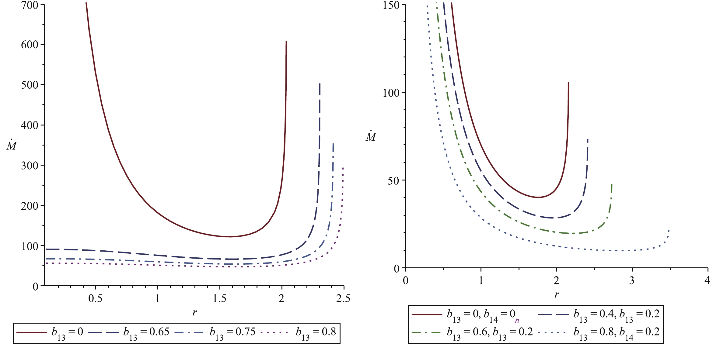
Figure 12. (color online) Contour plot of mass accretion rate for first kind (left panel) Einstein-aether BH with
$M=1, E_3=1, E_4=3$ and mass accretion rate for second kind (right panel) Einstein-aether BH with$M=1, E_3=1, E_4=2$ .The critical values and velocities for the Schwarzschild BH, first and second kind Einstein-aether BHs are shown in Tables 1, 2, and 3, respectively. From these tables, we observe that the critical radius increases for lower values of the EoS parameter.
k $r_c$ 

$u_c$ 

1 1.943298156 0.5072420898 1/2 1.997406813 0.5003244638 1/3 2.032863625 0.4959419894 1/4 2.057318666 0.4929855832 Table 1. Schwarzschild BH.
k $r_c$ 

$u_c$ 

1 1.579986833 0.8500828184 1/2 1.648351648 0.8038707229 1/3 1.692823135 0.7769197978 1/4 1.723345588 0.7596771055 Table 2. First kind Einstein-aether BH.
k $r_c$ 

$u_c$ 

1 1.922432132 0.6551340255 1/2 1.992969636 0.6389336505 1/3 2.038785465 0.6289719040 1/4 2.070201100 0.6223786150 Table 3. Second kind Einstein-aether BH.
-
We studied accretion of different fluids, including sub-relativistic, ultra-stiff, radiation, and ultra-relativistic fluids onto first and second kind Einstein-aether BHs within the framework of a Hamiltonian dynamical system. Results show that the pressure is exactly equal to the density for ultra-stiff fluids, and subsonic as well as supersonic accretion flow occurs. The pressure is half the density for ultra-relativistic fluids, where subsonic flow is followed by supersonic flow and vice versa. For radiation and sub-relativistic fluids, the pressure is lower than the density, and the fluid flow is similar to ultra-relativistic fluid for
$ v>0 $ .Furthermore, we discussed the behavior of the transonic solution for radiation, sub-relativistic, and ultra-relativistic fluids, where we observe that fluid flows form a closed orbit, which leads to possible homoclinic orbits in the second kind Einstein-aether BH in case of the subsonic solution. In contrast, the transonic solution exhibits a non-homoclinic orbit for the Schwarzschild BH and the first kind Einstein-aether BH. Interestingly, we observe the homoclinic orbits with superluminal motion for higher values of aether parameters and non-homoclinic orbits with superluminal motion for lower values of aether parameters near singularity of the second kind Einstein-aether BH, as
$ v > 1 $ . The critical radius$ r_c $ approaches singularity for the aforementioned fluids in the Schwarzschild BH as compared to the first and second kind Einstein-aether BH. This indicates that aether parameters play a critical role in the accretion process. We also investigated the behavior of the polytropic test fluid onto Einstein-aether BHs, where the accretion starts from subsonic/supersonic flow, and it does not pass through the saddle point for the first kind, whereas it passes through the saddle point for the second kind Einstein-aether BH. Interestingly, the accretion process ends in the region of the Killing horizon. These features are in agreement with Refs. [30, 41, 42]We formulated the general expression for the BH mass accretion rate (
$\dot {\rm{M}}$ ), energy density$ (\rho) $ , and the radial component of four-velocity$ (u^r) $ . We analyzed the BH mass accretion rate ($\dot {\rm{M}}$ ) in the presence of various fluids for Einstein-aether BHs and the Schwarzschild BH, which exhibits interesting signatures, as shown in Figs. 9, 10, 11, and 12. The mass accretion rate is higher in Einstein-aether BHs as compared to the Schwarzschild BH in case of the ultra-stiff fluid. For radiation, sub-relativistic, and ultra-relativistic fluids, the mass accretion rate is higher for the Schwarzschild BH than for the first and second kind Einstein-aether BH. Moreover, the maximum mass accretion rate occurs near the Killing horizon in the case of the first kind, whereas the maximum mass accretion rate is found near universal and Killing horizons in the case of the second kind of Einstein-aether BH. Finally, we calculated the critical radius$ r_c $ and critical velocities$ u_c $ for aforementioned fluids in Tables 1, 2 and 3.The present analysis examines the accretion process onto spherically symmetric non-rotating BHs in the Einstein-aether theory, which exhibits some particular signatures. As a further step in this line of research, the accretion of different fluids onto rotating BHs can be observed in both the Einstein-aether theory and Horava-Lifshitz theory [22, 23, 28], which may have highly diverse astrophysical and cosmological signatures. We conclude this study by emphasizing that the present analysis can be extended by considering chaplygin gas and generalized chaplygin gas accretion onto super massive BH. Moreover, an important application could be discussed regarding the stability of accretion flow at sufficiently closed distances. One further direction is to consider an axially symmetric but non-static geometry of the fluid.
The authors (A.J. and S.R.) are thankful to HEC, Islamabad.
Matter accretion onto Einstein-aether black holes via well-known fluids
- Received Date: 2019-10-21
- Accepted Date: 2020-02-05
- Available Online: 2020-06-01
Abstract: We study matter accretion onto Einstein-aether black holes by adopting the Hamiltonian approach. The general solution of accretion is discussed using the isothermal equation of state. Different types of fluids are considered, including ultra-relativistic, ultra-stiff, sub-relativistic, and radiation fluids, and the accretion process onto Einstein-aether black holes is analyzed. The behavior of the fluid flow and the existence of critical points is investigated for Einstein-aether black holes. We further discuss the general expression and behavior of polytropic fluid onto Einstein-aether black holes. The most important feature of this work is the investigation of the mass accretion rate of the above-mentioned fluids and the comparison of our findings with the Schwarzschild black hole, which generates particular signatures. Moreover, the maximum mass accretion rate occurs near the Killing and universal horizons, and the minimum accretion rate lies between them.


 DownLoad: