


 Abstract
 HTML
HTML Reference
 Related
 PDF
PDF


-
Charmonium physics plays a key role in the foundation of quantum chromodynamics (QCD), which is believed to be a fundamental theory for strong interactions. Owing to its intermediate energy scale and special features of QCD, both perturbative and non-perturbative physics appear within charmonium physics [1]. To date, the optimal way to study non-perturbative QCD is the lattice QCD, which is a quantum field theory defined on the discrete Euclidean space-time. Within this formalism, physical quantities are encoded in various Euclidean correlation functions, which in turn can be measured by performing Monte Carlo simulations [2, 3].
Recently, the two photon decay branching fractions for charmonium have been attracting considerable attention. Theoretically, this quantity is considered to provide a probe for the strong coupling constant at the charmonium scale. It has also been proposed as a sensitivity test for making corrections to the non-relativistic approximation via quark models or effective field theories, such as the non-relativistic QCD (NRQCD).
Furthermore, considerable progress has been made in recent years in the field of physics of charmonia via the investigations from various experimental collaborations, such as Belle, BaBar, CLEO-c, and BES [4–7]. Generically, there are two approaches to measure the two-photon branching fraction for charmonium: one by reconstructing the charmonium in light hadrons using two-photon fusion at
$ e^+e^- $ machines, and the other from$ p\bar{p} $ annihilation to charmonium.In this study, we calculate the two-photon decay width of the pseudoscalar and scalar charmonium, i.e.,
$ \Gamma(\eta_{c}\rightarrow\gamma\gamma) $ and$ \Gamma(\chi_{c0}\rightarrow\gamma\gamma) $ , in lattice QCD using two ensembles of$ N_f = 2 $ dynamical twisted mass fermion configurations that were generated by the European Twisted Mass Collaboration (ETMC). This ensures the so-called automatic$ {\cal{O}}(a) $ improvement for on-shell observables when the twisted mass fermions are at the maximal twist [8]. Lattice computation for the process$ \eta_c\rightarrow\gamma\gamma $ was perfomred using the same set of configurations in Ref. [9]. In this work, we consider$ \eta_c $ and$ \chi_{c0} $ simultaneously, since they mix with each other due to the lattice artifact of$ O(a^2) $ .This paper is organized as follows. In Sec. 2, the calculation strategy for the matrix element for two-photon decay of charmonium is reviewed, which is then related to the double-photon decay rates. We also outline the strategy for the mass spectrum and form factor of charmonium. To improve the signals of the corresponding correlation functions, we apply the variation method to construct the relevant interpolate operators. In Sec. 3, the simulation details are divided into several parts: In Sec. 3.1, we provide the parameters relevant with the configurations used in this study. In Sec. 3.2, the mass spectra of
$ \eta_c $ and$ \chi_{c0} $ are obtained. In Sec. 3.3, we present the results of the renormalization factor of the electromagnetic current operators. In Sec. 3.4, numerical results of the form factors are presented, which are then converted to the two photon decay width of$ \eta_c $ and$ \chi_{c0} $ . Final results for the decay widths are presented and compared with previous lattice computations and experiments. The discussion and conclusion are presented in Sec. 4. -
In this section, we briefly review the methods for the calculation of the two-photon decay rate of charmonium, which was presented in Ref. [10]. According to the Lehmann-Symanzik-Zimmermann (LSZ) reduction formula, we can express the amplitude for the two-photon decay of charmonium in the following form:
$ \begin{array}{*{20}{l}} {\langle \gamma ({q_1},{\iota _1})\gamma ({q_2},{\iota _2})|M({p_f})\rangle = - \mathop {\lim }\limits_{\scriptstyle{{q'}_1} \to {q_1}\atop \scriptstyle{{q'}_2} \to {q_2}}\epsilon _\mu ^*({q_1},{\iota _1})\epsilon_\nu ^*({q_2},{\iota _2})q_1'^2 q_2'^2 \displaystyle\int {{{\rm d}^4}} x{{\rm d}^4}y{\mkern 1mu} {{\rm e}^{{\rm i}{{q'}_1}.y + {\rm i}{{q'}_2}.x}}\langle \Omega |T\{ {A^\mu }(y){A^\nu }(x)\} |M({p_f})\rangle .} \end{array}$

(1) Here,
$ |\Omega\rangle $ denotes the QCD vacuum state; M represents either the$ \eta_c $ or$ \chi_{c0} $ meson state, depending on which one is calculated, and$ |M(p_f)\rangle $ is the corresponding meson state with four-momentum$ p_f $ , whereas$ |\gamma(q_i,\iota_i)\rangle $ ($ i = 1,2 $ ) is a single photon state that has the polarization vector$ \epsilon(q_i,\iota_i) $ with four-momentum$ q_i $ and helicity$ \iota_i $ . Then, treating the QED part perturbatively, we can replace the photon field operators by their corresponding current operators in QCD. We finally arrive at the following equation at the lowest order of QED,$ \begin{split} \langle \gamma(q_1, \iota_1)\gamma(q_2, \iota_2) | M(p_f) \rangle =& {(-e^2)} \mathop {\lim }\limits_{\scriptstyle{{q'}_1} \to {q_1}\atop \scriptstyle{{q'}_2} \to {q_2}} \epsilon_\mu^*({q_1},{\iota _1}) \epsilon^*_\nu(q_2, \iota_2) q_1'^2 q_2'^2 \displaystyle\int {\rm d}^4x {\rm d}^4y {\rm d}^4w\ {\rm d}^4z {\rm e}^{{\rm i} q'_1.y + {\rm i} q'_2.x}\, D^{\mu \rho}(y ,z) D^{\nu \sigma}(x, w) \langle\\ & \times \Omega | T\big\{ j_\rho(z) j_\sigma(w)\big\} | M(p_f)\rangle \end{split} $

(2) with
$ D^{\mu\nu}(y,z) $ being the free photon propagator. Basically, each initial/final photon state in the problem is replaced by the corresponding electromagnetic current operator that couples to the photon. Finally, a three-point function of the form$ \langle\Omega | T\big\{ j_\rho(z) j_\sigma(w)\big\} | M(p_f)\rangle $ needs to be computed, which is non-perturbative in nature and can be found using lattice QCD methods.Under certain conditions, Eq. (2) can be analytically continued from Minkowski space to Euclidean space, yielding
$ \begin{split} \langle\gamma(q_1, \iota_1) \gamma(q_2, \iota_2) |M(p_f)\rangle = & \lim\limits_{t_f-t \to \infty} e^2 \frac{ \epsilon_\mu(q_1, \iota_1) \epsilon_\nu(q_2, \iota_2)}{\dfrac{Z_{M}(p_f)}{2 E_{M}(p_f)} {\rm e}^{-E_{M}(p)(t_f-t)}} \int {\rm d}t_i {\rm e}^{- \omega_1 (t_i -t)}\\ & \langle \Omega | T\Big\{ \int {\rm d}^3 \vec{x}\, {\rm e}^{-{\rm i}\vec{p_f}.\vec{x}} \varphi_{M}(\vec{x}, t_f) \int {\rm d}^3 \vec{y}\, {\rm e}^{{\rm i}\vec{q_2}.\vec{y}} j^\nu(\vec{y}, t) j^\mu(\vec{0}, t_i)\Big\}|\Omega\rangle, \end{split} $

(3) where
$ \varphi_{M}(\vec{x}, t_f) $ is the field operator for the meson M;$ Z_{M}(p_f) $ is the spectral weight factor of the two-point function;$ \omega_1 $ is the energy for the photon at time-slice$ t_i $ ; and$ E_{M}(p_f) $ is the energy for the corresponding meson with momentum$ p_f $ . Then, the desired amplitude$ \langle\gamma(q_1, \iota_1) \gamma(q_2, \iota_2) | M(p_f)\rangle $ is obtained once the energies$ E_{M}(p_f) $ and the corresponding overlap matrix element$ Z_{M}(p_f) $ are known. These can be obtained from appropriate two-point functions. In this study, we use the variational method to find the optional interpolation operators to create/annihilate the$ \eta_c $ and$ \chi_{c0} $ meson states [11].Generally, an operator
$ {\cal{O}}^{\dagger}_i $ with definite$ J^{PC} $ can generate all the QCD eigenstates with the right quantum numbers$ \begin{array}{l} {\cal{O}}_i^\dagger|\Omega\rangle = \displaystyle\sum\limits_n|n\rangle\langle n|{\cal{O}}_i^\dagger|\Omega\rangle. \end{array} $

(4) To effectively generate the desired hadrons from vacuum, one could employ a basis of interpolators
$ {{\cal{O}}_i} $ that share the same quantum numbers and construct a two-point correlation function matrix as follows$ \begin{array}{l} C_{ij} = \langle\Omega|{\cal{O}}_i(t){\cal{O}}_j^\dagger(0)|\Omega\rangle. \end{array} $

(5) Here, the operators
$ {{\cal{O}}_i} $ are color-singlet constructions built from the basic quark and gluon fields of QCD. Then, we can express the correlation functions in the following form:$ \begin{array}{l} C_{ij} = \displaystyle\sum\limits_n\dfrac{1}{2E_n}\langle\Omega|{\cal{O}}_i(0)|n\rangle\langle n|{\cal{O}}_j^\dagger(0)|\Omega\rangle {\rm e}^{-E_nt}. \end{array} $

and the optimized interpolators are:
$ \begin{array}{l} \Omega_n^\dagger = \displaystyle\sum\limits_iv_i^n{\cal{O}}_i^\dagger. \end{array} $

(6) Therefore, the best estimate for the weights
$ v^n_i $ must be obtained according to the solution of the following generalized eigenvalue problem$ \begin{array}{l} C(t)v^n = \lambda_n(t)C(t_0)v^n. \end{array} $

(7) Here,
$ C(t) $ is the$ N\times{N} $ matrix whose elements are the correlation functions$ C_{ij}(t) $ constructed from the basis of N operators, and$ v^n $ is a generalized eigenvector. The generalized eigenvalues, or principal correlators,$ \lambda_n(t) $ , behave like${\rm e}^{-E_n(t-t_0)}$ at large times and can be used to determine the spectrum of the states. In practice, we solve Eq. (7) independently on each time-slice t, such that for each state n, we obtain a time series of generalized eigenvectors$ v^n(t) $ . We use$ v^n_i $ chosen on a single time-slice to construct the optimized operators in Eq. (6).Apart from the two-point functions of
$ \eta_c $ and$ \chi_{c0} $ , we also need the three-point functions$ G_{\mu\nu}(t_i,t) $ given by:$ \begin{split} G_{\mu\nu}(t_i,t) =& \langle 0 | T\Big\{ \int {\rm d}^3 \vec{x}\, {\rm e}^{-{\rm i}\vec{p_f}.\vec{x}} \varphi_{M}(\vec{x}, t_f)\\ &\times\int {\rm d}^3 \vec{y}\, {\rm e}^{{\rm i}\vec{q_2}.\vec{y}} j^\nu(\vec{y}, t) j^\mu(\vec{0}, t_i)\Big\}|0\rangle. \end{split} $

(8) We simulate
$ G_{\mu\nu}(t_i,t) $ on lattices across the temporal direction, while the sink of the meson is fixed. Then, we repeat this with a varying$ t_i $ to integrate across the three point function using an exponential weight${\rm e}^{-\omega_1{t_i}}$ , and then to extract the matrix element in Eq. (3). In particular, we use the optimized interpolators$ \Omega_n $ in Eq. (6) to generate the$ \eta_c,(n = 1) $ or$ \chi_{c0},(n = 2) $ state for the field interpolating operator$ \varphi_{M} $ in previous formulas.For the two photon decay of the
$ \eta_c $ meson, the matrix element$ \langle\gamma(q_1, \iota_1) \gamma(q_2, \iota_2) |M(p_f)\rangle $ in Eq. (3) can be parameterized using form factor$ F(Q_1^2,Q_2^2) $ as follows,$ \begin{split} &\langle\gamma(q_1, \iota_1) \gamma(q_2, \iota_2) |M(p_f)\rangle \\ = &2 \left(\dfrac{2}{3} e\right)^2 m_{\eta_c}^{-1} F(Q_1^2,Q_2^2)\epsilon_{\mu\nu\rho\sigma}\epsilon^{\mu}(q_1,\iota_1)\\&\times\epsilon^{\nu}(q_2,\iota_2)q_1^{\rho}q_2^{\sigma} ,\\ \end{split} $

(9) where
$ \epsilon_1, \epsilon_2 $ are the polarization vectors,$ Q_1^2,Q_2^2 $ are teh virtualities, and$ q_1, q_2 $ are the four-momenta for the two photons. The corresponding decay width can be expressed in terms of$ F(0,0) $ as follows,$ \begin{array}{l} \Gamma(\eta_c\rightarrow\gamma\gamma) = \pi \alpha_{em}^2 \dfrac{16}{81}m_{\eta_c} |F(0,0)|^2 \end{array} $

(10) with
$ \alpha_{em}\simeq 1/137 $ being the fine structure constant. Similarly, for$ \chi_{c0} $ , we have another form factor$ G(Q^2_1,Q^2_2) $ ,$ \begin{split} &\langle\gamma(q_1, \iota_1) \gamma(q_2, \iota_2) |M(p_f)\rangle \\ =& 2 \left(\dfrac{2}{3} e\right)^2 m_{\chi_{c0}}^{-1} G(Q_1^2,Q_2^2)\\&\times(\epsilon_1\cdot\epsilon_2q_1\cdot{q_2}-\epsilon_2\cdot{q_1}\epsilon_1\cdot{q_2})\\ \end{split} $

(11) with the decay width given by
$ \begin{array}{l} \Gamma(\chi_{c0}\rightarrow\gamma\gamma) = \pi \alpha_{em}^2 \dfrac{16}{81}m_{\chi_{c0}} |G(0,0)|^2\;. \end{array} $

(12) -
In this study, we utilize two ensembles with
$ N_f = 2 $ (degenerate u and d quarks) twisted mass configurations. These configurations are generated by the ETMC at the maximal twist to implement the so-called automatic$ {\cal{O}}(a) $ improvement [8]. The explicit parameters for these ensembles are presented in Ref. [12], and the two ensembles that we utilized are presented in Table 1. For the valence sector, we adopt the Osterwalder-Seiler setup, which introduces two extra twisted doublets for each non-degenerate quark flavor, namely,$ (u,d) $ and$ (c,c^{\prime}) $ with twisted masses$ a\mu_l $ and$ a\mu_c $ , respectively [13–17]. The explicit value of$ a\mu_l $ on Ens.$ \; B_1 $ is$ 0.004 $ , whereas it is$ 0.003 $ for Ens.$ \; C_1 $ . In this simulation, we use the physical mass of$ \eta_c $ to set the value of$ a\mu_c $ , yielding explicit values of$ 0.2542 $ and$ 0.2018 $ for Ens.$ \; B_1 $ and Ens.$ \; C_1 $ , respectively. In each doublet, the Wilson parameters have opposite signs ($ r = -r^{\prime} = 1 $ ). Performing an axial (or chiral) transformation, quark fields in the physical basis transform into the twisted basis [13]; i.e.,$ \beta $ 

a/fm $ V/{a^4} $ 

$ a\mu_{sea} $ 

$ m_{\pi} $ /MeV

$ m_{\pi}L $ 

$ N_{cfg} $ 

Ens. $ \; B_1 $ 

$ 3.9 $ 

0.085 $ 24^3\times{48} $ 

0.004 315 3.3 200 Ens. $ \; C_1 $ 

$ 4.05 $ 

0.067 $ 32^3\times{64} $ 

0.003 300 3.3 199 Table 1. Configuration parameters.
$ \begin{array}{rl} \left( \begin{array}{c} u\\ d \end{array}\right) = \hspace*{-3mm} & \exp({\rm i}\omega\gamma_5\tau_3/2)\left(\begin{array}{c} \chi_u\\ \chi_d \end{array}\right)\\ \left( \begin{array}{c} c\\ c^{\prime} \end{array}\right) = \hspace*{-3mm} & \exp({\rm i}\omega\gamma_5\tau_3/2)\left(\begin{array}{c} \chi_c\\ \chi_{c^{\prime}} \end{array}\right), \end{array} $

(13) where
$ \omega $ is the twist angle, and$ \omega = \pi/2 $ represents the maximal twist. Then, the left-side of the abovementioned equations correspond to quark fields in the physical basis, and the right-side correspond to quark fields in the twisted basis.Before writing the explicit form of the meson operators, one should exploit the symmetry properties of the twisted mass LQCD. We follow the discussion in reference [18] below. Isospin I and parity
$ {\cal{P}} $ are broken by$ {\cal{O}}(a^2) $ effects in the twisted mass LQCD. Meanwhile, a specific combination (i.e., light flavor exchange combined with parity) remains a symmetry of the twisted mass LQCD. We first write down the interpolating-field operators in the twisted basis and build the interpolating operators with the same Wilson parameters [16]. For the purpose of$ \eta_c $ and$ \chi_{c0} $ , we use two basis operators$ {\cal{O}}_1(x) = \bar{c}(x)\gamma_5{c}(x) $ ,$ {\cal{O}}_2 = \bar{c}(x){c}(x) $ . According to Eq. (13), the two basic operators in the twisted basis are given by$ {\cal{O}}_1 = \bar{\chi}_{c}{\chi_c} $ and$ {\cal{O}}_2 = \bar{\chi}_{c}\gamma_5{\chi_c} $ , which appear to have opposite parity. However, because twisted mass lattice QCD breaks parity, they in fact mix with each other. Taking into account this mixing is crucial. The solution of the generalized eigenvalue problem in Eq. (7) must be found to obtain the optimized operator that will create the$ \eta_c $ and$ \chi_{c0} $ meson from the vacuum. Without performing this generalized eigenvalue separation, the correct signal of$ \chi_{c0} $ cannot be observed in the two-point functions. The signal of$ \eta_c $ can naturally be observed even without considering this mixing effect, as it is the lightest state under consideration. -
The eigenvalue
$ \lambda_n $ in Eq. (7) corresponding with the corresponding meson state, i.e.,$ n = 1 $ represents$ \eta_c $ meson, and$ n = 2 $ represents the$ \chi_{c0} $ meson. Therefore, we use the anti-periodic boundary condition,$ \begin{split} \lambda_n(t, {{p}}_f)\stackrel{t\gg 1}{\longrightarrow}&\frac{|Z_{M}|^2}{E_{M}( {{p}}_f)}{\rm e}^{-E_{M}( {{p}}_f)\cdot\frac {T}{2}}\\ &\times\cosh\left[E_{M}( {{p}}_f)\cdot\left(\frac T2-t\right)\right]\;. \end{split} $

(14) In practice, we use eigenvalue
$ \lambda_1 $ with${{p}}_f = (0,0,0)$ to fit the spectral weight$ Z_{\eta_c} $ , and the explicit value of this factor is$ 0.4416(8) $ and$ 0.2675(3) $ on Ens.$ B_1 $ and Ens.$ C_1 $ , respectively. Meanwhile, we use eigenvalue$ \lambda_2 $ with${{p}}_f = (0,0,0)$ to fit the spectral weight$ Z_{\chi_{c0}} $ , and the explicit value of this factor is$ 0.6699(71) $ and$ 0.2983(33) $ on Ens.$ B_1 $ and Ens.$ C_1 $ , respectively. Thus, the mass can also be extracted from$ \begin{array}{l} \cosh(m_n) = \dfrac{\lambda_n(t-1)+\lambda_n(t+1)}{2\lambda_n(t)}, \end{array} $

(15) with
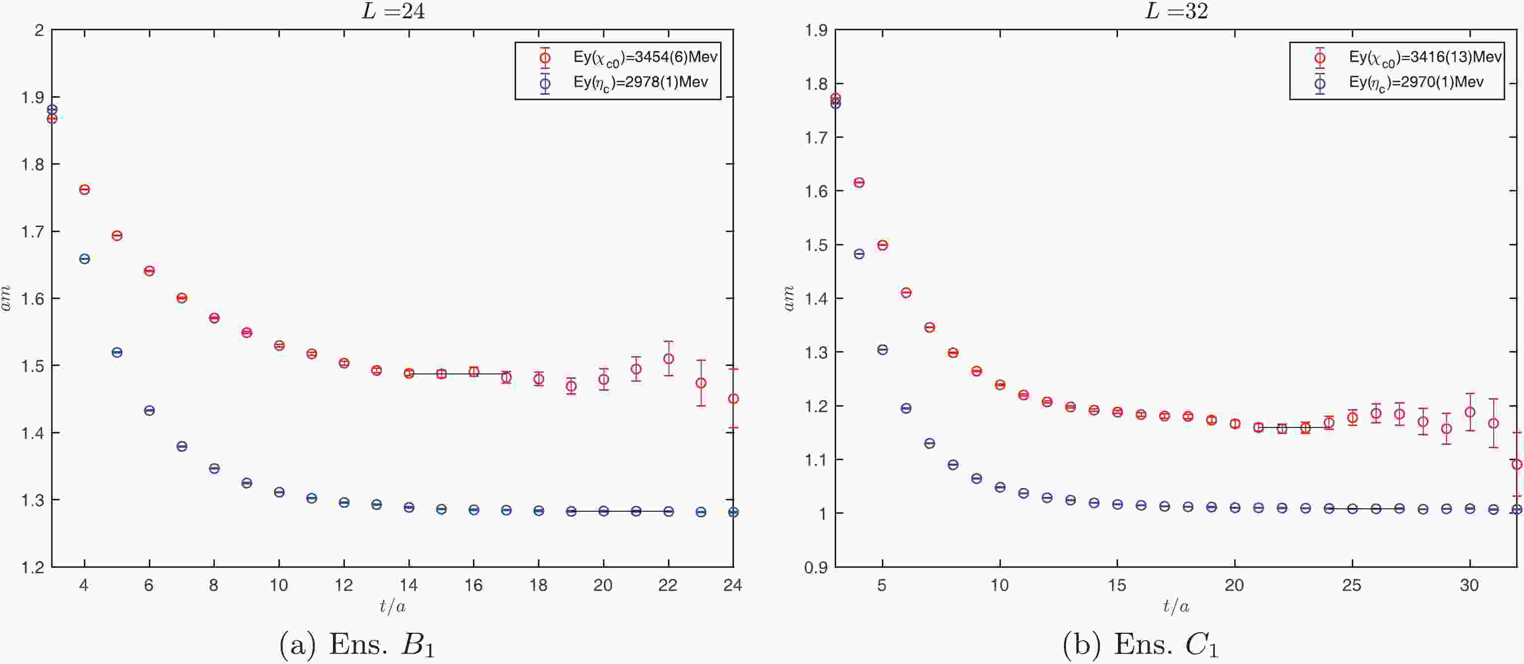
$ m_1 $ denoting the mass of$ \eta_c $ meson and$ m_2 $ that of$ \chi_{c0} $ . The effective mass plateaus of these mesons for Ens.$ B_1 $ and Ens.$ C_1 $ are illustrated in Fig. 1. From these mass plateaus, the masses of the mesons are determined, and the statistical errors are obtained using the jackknife method. The numerical results for the masses are summarized in Table 2. Notably, the mass values for$ \eta_c $ are utilized to fix the valence charm quark mass parameter$ a\mu_c $ . Therefore, only the masses of$ \chi_{c0} $ are predicted from this lattice computation.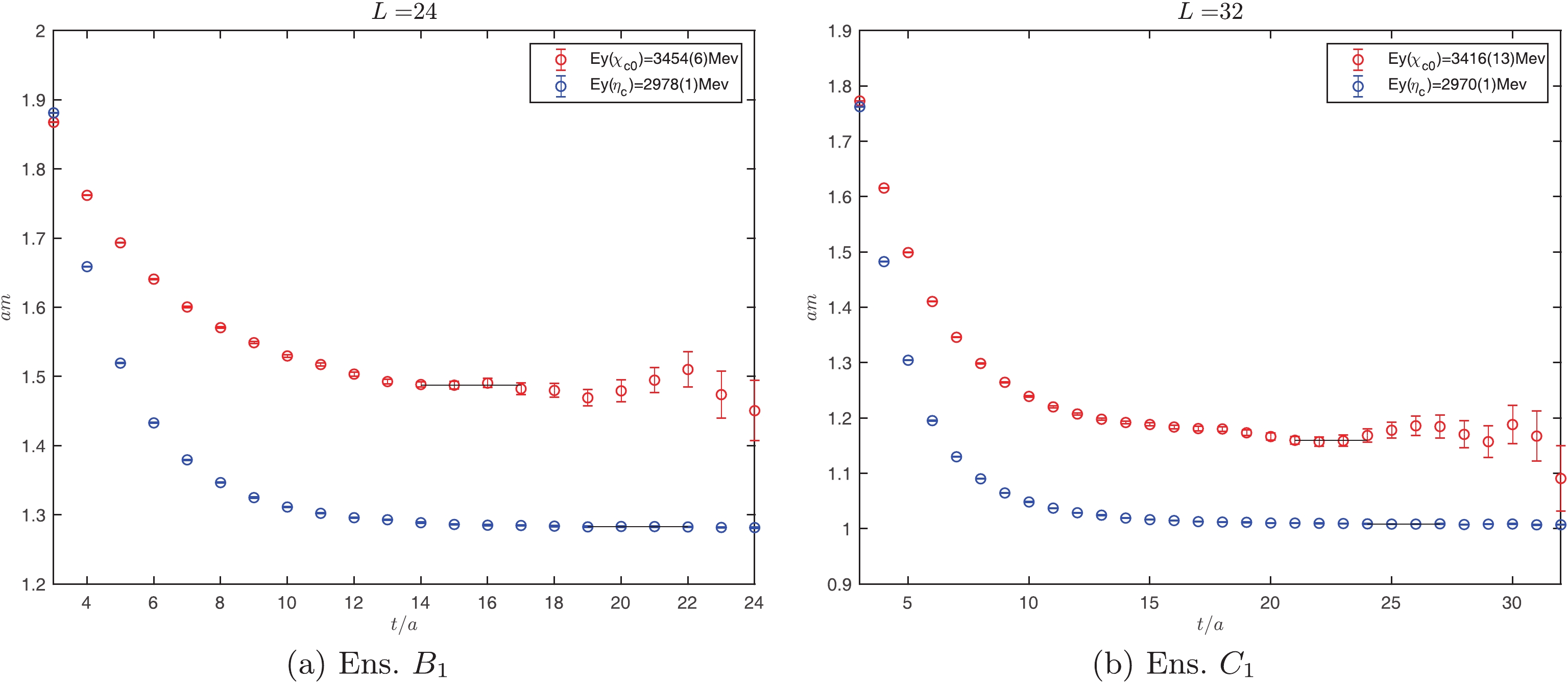
Figure 1. (color online) Mass plateaus of
$ \eta_c $ (blue point) and$ \chi_{c0} $ (red point) for Ens.$ B_1 $ and Ens.$ C_1 $ . The horizontal line segments denote the corresponding mass plateaus.$ \eta_c $ 

$ \chi_{c0} $ 

Ens. $ B_1 $ :

Mass/MeV 2978(1) 3454(6) Ens. $ C_1 $ :

Mass/MeV 2970(1) 3416(13) PDG: Mass/MeV 2983.9(5) 3414.71(30) Table 2. Mass values for
$ \eta_c $ and$ \chi_{c0} $ on Ens.$ B_1 $ and Ens.$ C_1 $ respectively. The last line cites the corresponding result from PDG [19].In principle, glueball states with the same quantum numbers are also present in a similar energy range [20]. However, in this lattice calculation, we have only utilized the quark bilinear operators for charmonium states and did not observed the sign of the glueballs.
-
The current operators in Eq. (8) are electromagnetic current operators. In principle, they contain all the flavors of quarks weighted by the corresponding charges. Light quark flavors will only enter the question via disconnected diagrams, which are neglected in this study. When considering the charm quark, we only need to consider the current
$ \bar{c}\gamma_\rho c(x) $ . A subtlety in the lattice computation is that, with$ c(x)/\bar{c}(x) $ being the bare charm/anti-charm quark field on the lattice, composite operators such as the current$ j_\rho(x) = Z_V\bar{c}(x)\gamma_{\rho}c(x) $ need an extra multiplicative renormalization factor$ Z_V $ , which can be extracted by the ratio of two-point function with respect to the three-point function for$ \eta_c $ [21]:$ \begin{array}{l} Z_V^{\mu} = \dfrac{p^{\mu}}{E(p)}\dfrac{(1/2)\Gamma_{\eta_c}^{(2)}}{\Gamma^{(3)}_{\eta_c}}, \end{array} $

(16) where
$ \mu $ is the Dirac index, which we assume to be zero.$ \Gamma_{\eta_c}^{(2)} $ and$ \Gamma^{(3)}_{\eta_c} $ are the two point correlation function and three point correlation function relevant to$ \eta_c $ , respectively. The explicit forms are:$ \begin{array}{l} \Gamma_{\eta_c}^{(2)} = \displaystyle\sum\limits_{ { x}}{\rm e}^{-{\rm i} {{p}}\cdot { x}}\langle{\cal{O}}_{\eta_c}( { x}, t){\cal{O}}_{\eta_c}^{\dagger}(0, 0)\rangle ,\end{array} $

(17) $ \begin{array}{l} \Gamma_{\eta_c}^{(3)} = \displaystyle\sum\limits_{ { x}, { y}}{\rm e}^{-{\rm i} {{p}}_f\cdot { x}}{\rm e}^{{\rm i} {{q}}\cdot { y}}\langle{\cal{O}}_{\eta_c}( { x}, t_f)\bar{c}\gamma_0{c}( { y},t){\cal{O}}_{\eta_c}^{\dagger}(0, 0)\rangle ,\\ \end{array} $

(18) with
$ {\cal{O}}^\dagger_{\eta_c} $ and$ {\cal{O}}_{\eta_c} $ creating and annihilating a state with the quantum number of$ \eta_c $ meson, respectively. Indeed, we use the simple local operator, i.e.,$ \bar{c}\gamma_5{c} $ . According to Eq. (16), we can obtain the multiplicative renormalization factor$ Z_V $ , which we have shown in Fig. 2. The values of the renormalization factor$ Z_V $ are$ 0.6296(18) $ and$ 0.6476(61) $ for Ens.$ B_1 $ and Ens.$ C_1 $ , respectively.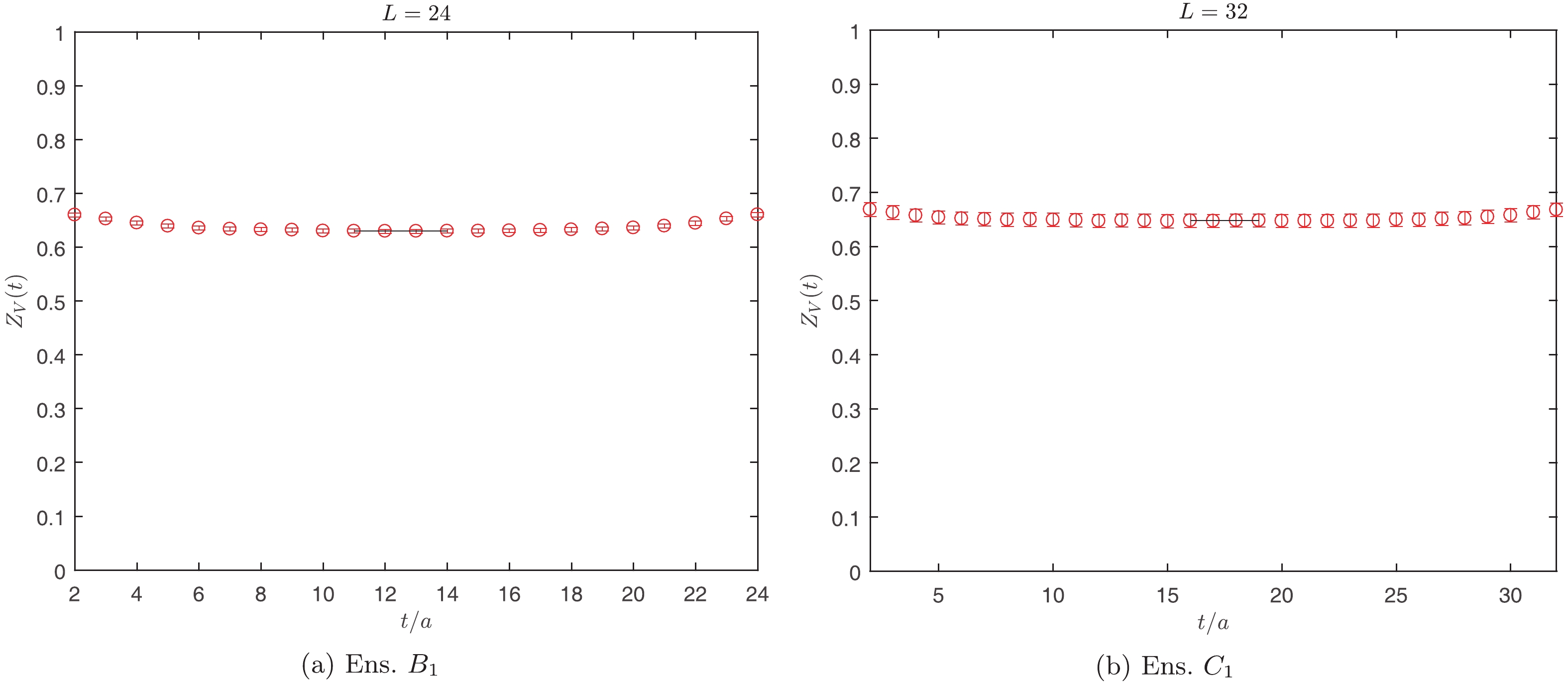
Figure 2. (color online) Renormalization factors
$ Z_V $ for Ens.$ B_1 $ and Ens.$ C_1 $ . The horizontal line segments denote the corresponding values for$ Z_V $ . -
To compute the relevant matrix element in Eq. (3), we place the meson at a fixed sink position
$ t_f $ , which is chosen to be$ 24 $ for Ens.$ B_1 $ and$ 32 $ for Ens.$ C_1 $ . These sinks are then used as a sequential source for a backward propagator inversion. This allows us to investigate all the possible source positions$ t_i $ . We can then freely vary the values of$ \omega_1 $ and$ Q^2_1 $ , and inspect the integrand as a function of$ t_i $ in Eq. (3) for a given insertion position t. As an example, in Fig. 3 and Fig. 4, we show the integrand for the insertion positions$ t = 4,8,12,16,20 $ for Ens.$ B_1 $ and$ t = 4,8,12,16,20,24,28 $ for Ens.$ C_1 $ with a particular value$ \vec{p}_f = (000) $ for$ \eta_c $ and$ \chi_{c0} $ .
Figure 4. (color online) Integrand for insertion positions obtained from simulations on Ens.
$ B_1 $ (left figure), and Ens.$ C_1 $ (right figure) respectively. We take$ n_2 = (0 0 -3) $ ;$ n_f = (0\ 0\ 0) $ as an example. The insertion positions for lattice size:$ 24^3\times48 $ and lattice size:$ 32^3\times64 $ are$ t = 4,\; 8,\; 12,\; 16,\; 20 $ and$ t = 4,\; 8,\; 12,\; 16,\; 20,\; 24,\; 28 $ respectively.
Figure 5. (color online) Distribution of virtualities
$ (Q^2_1,Q^2_2) $ (lattice units) for Ens.$ C_1 $ computed for$ \eta_c $ (left panel) and$ \chi_{c0} $ (right panel).The computation must cover the physical kinematic regions of interest. For this purpose, we must scan the corresponding parameter space of the two virtualities
$ Q^2_1 $ and$ Q^2_2 $ . Basically, we follow the following strategy: we first fix the four-momentum of$ \eta_c $ and$ \chi_{c0} $ ,$p_f = (E, {{p}}_f)$ and place it on a given time-slice$ t_f = T/2 $ . In this simulation, we only compute the case of${{p}}_f = (0,0,0)$ , and E is simply the mass of the$ \eta_c $ or$ \chi_{c0} $ meson. Then, we judiciously choose several values of virtuality$ Q^2_1 $ around the physical point$ Q^2_1 = 0 $ . To be specific, we pick the range$ Q^2_1\in [-0.5,+0.1] $ GeV$ ^2 $ on Ens.$ B_1 $ and$ Q^2_1\in [-0.5,+0.1] $ GeV$ ^2 $ on Ens.$ C_1 $ , which satisfies the constraint$ Q^2_1>-m^2_\rho $ [9]. For a given${{p}}_f$ , a choice of${{q}}_1$ completely specifies${{q}}_2$ due to${{p}}_f = {{q}}_1+ {{q}}_2$ . Therefore, we take several choices of${{q}}_1 = {{n}}_1(2\pi/L)$ by changing three-dimensional integer${{n}}_1$ . Then the energy of the first photon is also obtained using either the continuum or the lattice dispersion relations as follows:$ \begin{array}{l} \omega^2_1 = {{q}}^2_1-Q^2_1\;, \end{array} $

(19) $ \begin{array}{l} 4\sinh^2(\omega_1/2) = 4\displaystyle\sum\limits_i\sin^2( {{q}}_{1i}/2)-\hat{Q}^2_1\;, \end{array} $

(20) where
$ \hat{Q}^2_1 = 4\sinh^2(Q_1/2) $ is the lattice version for the virtuality. Apparently, we can also compute the virtuality of the second photon, since both$ \omega_2 $ and${{q}}_2$ are constrained by the energy-momentum conservation. One has to make sure that the values of$ Q^2_2 $ thus computed do satisfy the constraint$ Q^2_2>-m^2_\rho $ , otherwise it is omitted. This procedure is summarized as follows:1. Judiciously choose several values of
$ Q^2_1 $ in a suitable range. We picked seven values of$ Q^2_1 $ ;2. Pick different values of
${{n}}_1$ , such that${{q}}_1 = {{n}}_1(2\pi/L)$ . As described above, this fixes both$ \omega_1 $ and$ Q^2_2 $ using the energy-momentum conservation. This is done using either the continuum or the lattice dispersion relations. To be specific, for each$ Q^2_1 $ , we picked four different${{q}}_1$ ;3. Make sure all the values of
$ Q^2_1,Q^2_2 >-m^2_\rho $ , otherwise the choice is simply ignored;4. For each validated choice above, compute the three-point functions (8) and obtain the hadronic matrix element using Eq. (3).
In this approach, we have obtained a total of 28 points on the
$ (Q^2_1,Q^2_2) $ plane around the origin. As an example, the distribution of these virtualities for the two mesons are shown in Fig. 5 for the case of lattice dispersion relations. One could also peform the same procedure using the conventional continuum dispersion relations. The difference of these two approaches will ultimately provide us with an estimate of the finite lattice spacing error of the calculation.
Figure 3. (color online) Integrand for insertion positions obtained from simulations on Ens.
$ B_1 $ (left figure), and Ens.$ C_1 $ (right figure). We take$ n_2 = (-1 -1 -2) $ ;$ n_f = (0\ 0\ 0) $ as an example. The insertion positions for lattice size:$ 24^3\times48 $ and lattice size:$ 32^3\times64 $ are$ t = 4,\; 8,\; 12,\; 16,\; 20 $ and$ t = 4,\; 8,\; 12,\; 16,\; 20,\; 24,\; 28 $ , respectively.In our real lattice QCD computation, the integration of
$ t_i $ in Eq. (3) is replaced by discrete summation over$ t_i $ using the trapezoid rule. The resulting values exhibit a plateau behavior with respect to t, which is then utilized to extract the corresponding form factor. In this approach, we have obtained numerical results for$ F(Q^2_1,Q^2_2) $ and$ G(Q^2_1,Q^2_2) $ at 28 different points in the plane of the two virtualities. As an example, the form factor plateaus for$ \eta_c $ are illustrated in Fig. 6 for the case of$Q_1^2 = 0\; {\rm GeV}^2$ . The corresponding case for$ \chi_{c0} $ is shown in Fig. 7.
Figure 6. (color online) Plateaus of pseudoscalar form factors obtained from integration of
$ t_i $ for three point function$ G_{\mu\nu}(t_i,t) $ with Ens.$ B_1 $ (left figure) and Ens.$ C_1 $ (right figure). We take$Q_1^2 = 0\; {\rm GeV}^2$ ;$ n_f = (0\ 0\ 0) $ as an example. The errors in these figures are estimated using the conventional jack-knife method.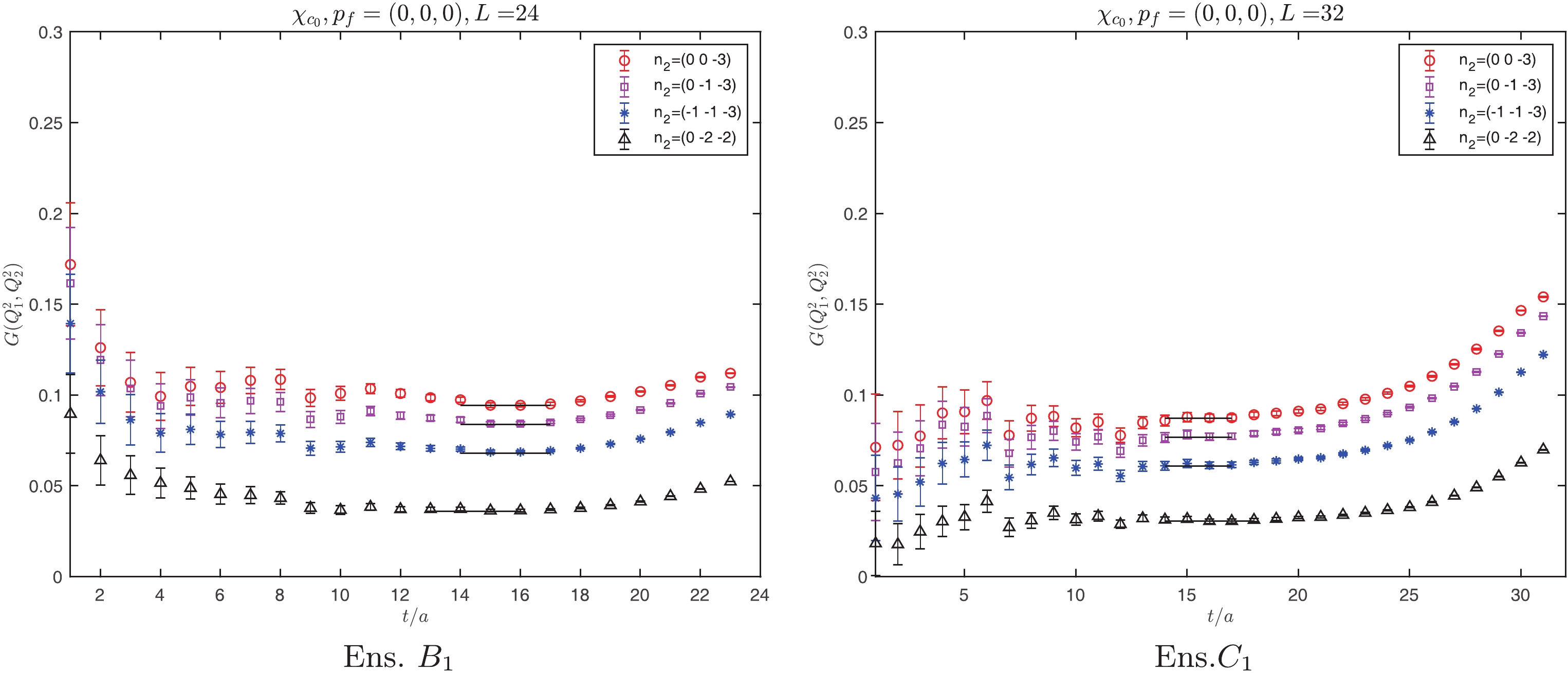
Figure 7. (color online) Plateaus of scalar form factor obtained from integration of
$ t_i $ for three point function$ G_{\mu\nu}(t_i,t) $ with Ens.$ B_1 $ (left figure) and Ens.$ C_1 $ (right figure). We take$Q_1^2 = 0\; {\rm GeV}^2$ ;$ n_f = (0\ 0\ 0) $ as an example. The errors in these figures were estimated using the conventional jack-knife method. -
To obtain the physical decay width, we only need the values of the form factors at the physical photon point, namely
$ Q^2_1 = Q^2_2 = 0 $ . Fig. 5 shows the distribution of the 28 data points in the$ (Q^2_1,Q^2_2) $ plane, and we could implement cuts in the plane. For a given value of$ Q^2_{\rm cut}>0 $ , we select the points that satisfy the following inequality:$ \begin{array}{l} \sqrt{(Q^2_1)^2+(Q^2_2)^2} \leqslant Q^2_{\rm cut}\;. \end{array} $

(21) Evidently, taking a large enough
$ Q^2_{\rm cut} $ will allow all of the points be considered, while selecting a smaller value for$ Q^2_{\rm cut} $ will account for only those points, whose distances are closer than$ Q^2_{\rm cut} $ . In contrast, for a given value of$ Q^2_{\rm cut} $ , we could utilize a different fitting formula to obtain the corresponding values of the form factor. Because it is the value at the origin that is directly related to the decay width, it is natural to use a polynomial type of fit in both$ Q^2_1 $ and$ Q^2_2 $ . Furthermore, due to boson symmetry, this function must be symmetric with respect to$ Q^2_1 $ and$ Q^2_2 $ . Therefore, by varying the cut value$ Q^2_{\rm cut} $ and various orders of polynomials in the virtualities, we could investigate the values of the form factors at the physical point.To be specific, we adopt a polynomial ansatz up to
$ Q^2_1 $ and$ Q^2_2 $ to the third power to fit the data of the form factor. For the$ \eta_c $ meson, we use:$ \begin{split} F(Q_1^2,Q_2^2) =& a_0+a_1(Q_1^2+Q_2^2) \\ &+a_2(Q_1^4+Q_2^4)+a_3Q_1^2Q_2^2 \\& +a_4(Q_1^6+Q_2^6)+a_5(Q_1^2Q_2^4+Q_2^2Q_1^4)\;, \end{split} $

(22) and we apply a similar form for the
$ \chi_{c0} $ form factor$ G(Q^2_1,Q^2_2) $ . Notably,$ a_0\equiv F(0,0) $ is the form factor at the physical photon point, which is directly related to the decay width of the meson. Polynomial forms with less terms, i.e., with only up to first or second powers in$ Q^2_1 $ and$ Q^2_2 $ , have also been attempted. This implies that we are fitting the data points with$ 2 $ ,$ 4 $ , and$ 6 $ parameters, respectively, as terms at the same orders of$ Q^2_1 $ and$ Q^2_2 $ must be included or excluded on the same footing. Correlated fits are performed in all the cases. Depending on the number of points considered, which is controlled by$ Q^2_{\rm cut} $ , and the number of terms kept in the fitting polynomial, we finally arrive at the values for the form factors at the origin, namely$ F(0,0) = a_0 $ for both the ensembles. Similar procedures have been implemented as well for$ \chi_{c0} $ , resulting in the values for$ G(0,0) $ .The fitting procedures described above can be implemented using either the continuum or lattice version of the dispersion relations, as indicated in Eq. (19) or Eq. (20). The procedure can be performed for either the pseudo-scalar or scalar meson on either of the two ensembles utilized in this calculation. Therefore, we perform the fitting procedure in eight different cases. The difference between the corresponding results obtained from different dispersion relations will then inform us about the lattice artifacts of the calculation.
As an illustration, in Fig. 8, the fitting results for
$ \eta_c $ and$ \chi_{c0} $ on Ens. C1 using lattice dispersion relations are shown. Here the horizontal axis denotes the cut values$ Q^2_{\rm cut} $ , while the vertical axis represents the values for$ F(0,0) $ or$ G(0,0) $ together with the errors (data points with error-bars). For each fixed value of$ Q^2_{\rm cut} $ , we have performed three fits with$ 2 $ ,$ 4 $ , and$ 6 $ parameters. These three points are shifted horizontally by a small amount to make them recognizable. The corresponding values of$ \chi^2/\rm{dof} $ for each fit are also shown as points without error-bars. By inspecting the plot, we obtain an estimate regarding the consistency and quality of these different fits, and the differences among the values of$ F(0,0) $ can also offer us an estimate of the systematics for the fitting procedure.
Figure 8. (color online) Fiting results for
$ \eta_c $ and$ \chi_{c0} $ on Ens. C1 using lattice dispersion relations. The horizontal axis denotes the cut values$ Q^2_{\rm cut} $ , while the vertical axis denotes the values for$ F(0,0) $ or$ G(0,0) $ together with the errors (data points with error-bars). The integers in brackets along the horizontal axis indicate the number of data points below$ Q^2_{\rm cut} $ . Points without errors show the corresponding values of$ \chi^2 $ /dof, the values that are obtained to the right edge of each box.Having obtained these eight plots, we proceed as follows:
● For each of these plots, taking the example above, we pick the case with lowest value of
$ \chi^2/\rm{dof} $ as the final result for$ F(0,0) $ together its statistical error in this particular case.● We further attribute a systematic error arising from the fitting procedure by taking the largest difference in the central values of
$ F(0,0) $ with comparable$ \chi^2/\rm{dof} $ . This then yields the result for$ F(0,0) $ with a certain type of dispersion relations on a particular ensemble.● By comparing the difference in
$ F(0,0) $ between the two different dispersion relations, we further assign a systematic error, which is taken to be the difference between the two values, arising from the lattice spacing.● A similar procedure can be applied to
$ \chi_{c0} $ as well.In this way, we obtain the results of
$ F(0,0) $ and$ G(0,0) $ on two ensembles, as explicitly listed below:$ F(0,0)_{B1} = 0.1283(1)(3)(77)\;, $

(23) $ F(0,0)_{C1} = 0.1240(4)(13)(68)\;, $

(24) $ G(0,0)_{B1} = 0.1017(7)(102)(126)\;, $

(25) $ G(0,0)_{C1} = 0.0907(8)(19)(90)\;, $

(26) In these expressions, the first error is statistical, the second is the error from the fitting procedure described above, and the third is the finite lattice error estimated using the two different dispersion relations. Evidently, in all the cases, the results are dominated by systematic errors, especially the finite lattice spacing errors. In fact, the results on the two different ensembles are consistent within this estimate of finite lattice spacing errors. We therefore decide not to make any continuum extrapolations. The computations with more values of lattice spacings will clearly be crucial to determine these large lattice spacing errors.
To compare with the previous lattice computations, we note that the result for
$ \Gamma(\eta_c\rightarrow\gamma\gamma) $ is slightly larger than the previous result presented in Ref. [9] when the same set of configurations were used. This difference is attributed to the fact that the mixing of$ \eta_c $ and$ \chi_{c0} $ in the twisted mass setup was not fully disentangled in the previous calculation in Ref. [9]. In the case where a properly chosen operator that mixes with both the$ \eta_c $ -like and$ \chi_{c0} $ -like interpolating operators is not used, it would not be possible to observe the correct$ \chi_{c0} $ signal as discussed at the end of subsection 3.1.Finally, we convert the results in the form factors into their corresponding ones in the decay widths. We simply add all the errors in the form factors in the quadrature and neglect the ones in the mass of the mesons. This then leads to the following results for the decay widths:
$ \begin{split} \Gamma(\eta_c\rightarrow\gamma\gamma)_{B1} =& 1.62(19)\;\rm KeV , \\ \Gamma(\eta_c\rightarrow\gamma\gamma)_{C1} =& 1.51(17)\;\rm KeV , \\ \Gamma(\chi_{c0}\rightarrow\gamma\gamma)_{B1} = & 1.18(38)\;\rm KeV , \\ \Gamma(\chi_{c0}\rightarrow\gamma\gamma)_{C1} =& 0.93(19)\;\rm KeV . \end{split} $

(27) These are to be compared with the following values given by PDG:
$ \begin{split} \Gamma(\eta_c\rightarrow\gamma\gamma)_{\rm PDG} =& 5.02(51) \rm KeV , \\ \Gamma(\chi_{c0}\rightarrow\gamma\gamma)_{\rm PDG} =& 2.20(22) \rm KeV . \end{split} $

(28) These numbers are all in the same ballpark as the experimental ones, although they remain somewhat smaller. However, because no controlled continuum extrapolations have been performed yet, it is still premature to draw any conclusions for the discrepancy. Our large estimated finite lattice errors offer some hint that this might be the major source of errors. In the future, more studies should be conducted at different lattice spacings to control the lattice artifacts in a systematic manner. Another source of systematic errors could come from the mixing with the nearby glueball states. Thus far, no lattice calculations have considered such an effect. Considerable efforts are needed in the future to take the aforementioned factors into account.
-
In this exploratory study, we calculate the two-photon decay width for
$ \eta_c $ and$ \chi_{c0} $ using unquenched$ N_f = 2 $ twisted mass fermions. The computation is performed with two lattice ensembles (coarser and finer) at two different lattice spacings. The mass spectra for the$ \eta_c $ and$ \chi_{c0} $ meson state are obtained by solving a generalized eigenvalue problem, which disentangles parity mixing between the two mesons.Our results for the decay width
$ \Gamma(\eta_c\rightarrow\gamma\gamma) $ and$ \Gamma(\chi_{c0}\rightarrow\gamma\gamma) $ are summarized in Eq. (27) for the two ensembles utilized in this computation. With these two ensembles, we only estimate the finite lattice spacing errors for each ensemble, and no continuum extrapolations are performed. Albeit without the continuum extrapolations, our results are in the right ballpark as the PDG values shown in Eq. (28).In the future, lattice calculations with more values of lattice spacings are certainly required to control the finite lattice spacing errors, which appear to be a dominant source. Meanwhile, the disconnected contributions will be a good supplement to this study. Possible mixing with the gluonic excitations must also be addressed. It will also be helpful to research unquenched configurations with other ensembles or other methods. We also expect to obtain more precise experiments to be performed on double-photon decays of charmonium.
The authors thank the European Twisted Mass Collaboration (ETMC) for allowing us to use their gauge field configurations. Our thanks also go to the National Supercomputing Center in Tianjin (NSCC).
Lattice study of two-photon decay widths for scalar and pseudo-scalar charmonium
- Received Date: 2020-03-25
- Available Online: 2020-08-01
Abstract: This exploratory study computes two-photon decay widths of pseudo-scalar (


 DownLoad: