


 Abstract
 HTML
HTML Reference
 Related
 PDF
PDF


-
The relativistic hydrodynamic theory provides a good description of the space-time evolution and many non-equilibrium properties of quark-gluon plasma (QGP) produced in heavy ion collisions at the Relativistic Heavy Ion Collider (RHIC) and the Large Hadron Collider (LHC) [1-4].
There has been excellent progress in solving relativistic viscous hydrodynamics equations analytically with different approximations and special symmetries as well as numerically in the recent years [5-36]. These analytical solutions play a very important role in understanding the evolution dynamics and are good testbeds for numerical solutions.
Recently, a series of interesting analytical solutions for longitudinally expanding relativistic perfect fluid were found by the Budapest and Wuhan group [16, 18, 21-23]. These ideal hydrodynamics solutions combined with the Buda-Lund model [37] have been utilized for simulating QGP medium dynamic evolution and readily reproduced the observed final state multiplicity distribution and its dependence on beam energy, collision system, particle mass, and freeze-out temperature [14, 16, 19, 21, 23, 38, 39].
However, a substantial comparison between the experimental data and the viscous hydrodynamic simulations found that QGP is a nearly perfect fluid, but it contains a small specific shear viscosity. The shear viscosity ratio of QGP is very close to the lower bound
$ 1/4\pi $ computed for$ {\cal{N}} = 4 $ super-Yang-Mills (SYM) theory in the AdS/CFT correspondence [40-43]. In this study, we will go beyond both the Csörgő-Nagy-Csanád (CNC) solutions and the Csörgő-Kasza-Csanád-Jiang (CKCJ) solutions of the relativistic perfect fluid for longitudinally expanding fireballs [16, 18, 22] and present a perturbation analytical solution of the longitudinally expanding first-order (Navier-Stokes limit) viscous hydrodynamic equations. Furthermore, we present the numerical results of the second-order (Israel-Stewart limit) viscous hydrodynamics equations as a part of the longitudinally expanding fireballs theory based on the assumption of a small relaxation time [44]. We find that small shear pressure tensor relaxation time$ \tau_{\pi} $ approximation solves the instability problem of the first-order approximation, indicating the stability of the second-order numerical results. This study provides a self-consistent first-order and second-order viscous hydrodynamics with longitudinally expanding dynamics. It can provide a better understanding of the relationship between the viscosity effect and longitudinal acceleration effect for the medium evolution in future phenomenological studies.The remainder of this paper is organized as follows. In Sec. 2, the 2nd viscous hydrodynamic equations are reconstructed in Rindler coordinates according to the Landau-Lifshitz formalism [11], and perturbation solutions are presented. In Sec. 3, numerical results of viscous hydrodynamics for longitudinally expanding fireball are investigated. Brief summary and discussion are given in Sec. 4.
-
We focused on the so-called Rindler-coordinates for which
$ \tau = \sqrt{t^{2}-r^{2}} $ is the proper time and$ \eta_{s} = 0.5\ln [(1+r/t)/(1-r/t)] $ is the space-time rapidity, where$ x^\mu = (t,r_1,\dots,r_d) $ and$ r = \sqrt{\Sigma_i r_i^2} $ [16, 18, 22]. We consider (1+1) dimensional fluid flow in (1+3) dimensional space-time since we focus on the perturbation solutions of a longitudinal expanding fireball with shear viscosity. The flow 4-velocity field$ u^{\mu} $ in the cartesian coordinates (the Minkowski flat space-time) for this system is$ u^{\mu} = (\cosh\Omega, 0, 0, \sinh\Omega), $

(1) where flow rapidity
$ \Omega $ is a function of space-time rapidity$ \eta_{s} $ and is independent of proper time$ \tau $ [18], with the 4-velocity normalized as$ u^{\mu}u_{\mu} = 1 $ . The second-order hydrodynamic equations without external currents are simply given by$ \partial_{\mu} T^{\mu\nu} = 0, $

(2) with the energy-momentum tensor
$ T^{\mu\nu} \!=\! \varepsilon u^{\mu}u^{\nu} \!-\!p \Delta^{\mu\nu} \!+\! \pi^{\mu\nu} $ , where$ \varepsilon $ is the energy density, p is the pressure,$ g_{\mu\nu} $ =$ {\bf{diag}} $ $ (1,-1,-1,-1) $ the metric tensor, and$ \Delta^{\mu\nu} = g^{\mu\nu}-u^{\mu}u^{\nu} $ the projection operator which is orthogonal to the fluid velocity. The shear pressure tensor$ \pi^{\mu\nu} $ represents the deviation from ideal hydrodynamics and local equilibrium, it satisfies$ u^{\mu}\pi_{\mu\nu} = 0 $ and is traceless$ \pi^{\mu}_{\; \mu} = 0 $ in the Landau frame.The energy density and pressure are related to each other by the equation of state (EoS),
$ \varepsilon = \kappa p, $

(3) where
$ \kappa $ is usually related to the local temperature [44], in this case we assume$ \kappa $ to be a constant and independent of the temperature.The fundamental equations of viscous fluid dynamics are established by projecting appropriately the conservation equations of the energy momentum tensor (Eq. (2)). The conservation equations can be rewritten as,
$ D\varepsilon = -(\varepsilon+p)\theta+\sigma_{\mu\nu}\pi^{\mu\nu}, $

(4) and
$ (\varepsilon+p)Du^{\alpha} = \nabla^{\alpha}p+\pi^{\alpha\mu}Du_{\mu}-\Delta^{\alpha\nu}\nabla^{\mu}\pi_{\mu\nu}, $

(5) respectively, where
$ D = u^{\mu}\partial_{\mu} $ is the comoving derivative and$ \theta = \partial_{\mu}u^{\mu} $ is the expansion rate.In terms of the 14-moment approximation result from [7, 45],
$ \partial_{\mu}s^{\mu}\geqslant 0 $ reduces the corresponding thermodynamic forces. The general traceless shear tensor$ \pi^{\mu\nu} $ is [7, 41],$ \begin{split} \pi^{\mu\nu} =& 2\eta\sigma^{\mu\nu}-\tau_\pi \left[ \Delta^\mu_\alpha\Delta^\nu_\beta u^\lambda \nabla_\lambda \pi^{\alpha\beta} +\frac{1}{3}\pi^{\mu\nu} \theta\right] \\&- \lambda_1 \pi^{\langle\mu}_{\ \ \lambda} \pi^{\nu\rangle\lambda}-\lambda_2 \pi^{\langle \mu}_{\ \ \lambda} \Omega^{\nu\rangle\lambda}- \lambda_3 \Omega^{\langle \mu}_{\ \ \lambda}\Omega^{\nu\rangle \lambda}, \end{split} $

with the symmetric shear tensor
$ \sigma^{\mu\nu} $ and the antisymmetric vorticity tensor$ \Omega^{\mu\nu} $ defined as$ \sigma^{\mu\nu}\equiv\left(\frac{1}{2}(\Delta^{\mu}_{\alpha}\Delta^{\nu}_{\beta}+\Delta^{\mu}_{\beta}\Delta^{\nu}_{\alpha}) -\frac{1}{3}\Delta^{\mu\nu}\Delta_{\alpha\beta}\right)\partial^{\alpha}u^{\beta}, $

(6) $ \Omega^{\mu\nu}\equiv \frac{1}{2}\Delta^{\mu\alpha}\Delta^{\nu\beta}(\nabla_\alpha u_\beta -\nabla_\beta u_\alpha), $

(7) where
$ \eta $ ,$ \tau_{\pi} $ ,$ \lambda_{1} $ ,$ \lambda_{2} $ ,$ \lambda_{3} $ are positive transport coefficients in the flat space time.$ \eta $ is the shear viscosity coefficient, and$ \tau_{\pi} $ is the relaxation time for shear pressure tensor corresponding to the dissipative currents, respectively. Shear viscosity ratio$ \eta/s $ of the QGP is very close to the lower bound of$ 1/4\pi $ computed for a strongly coupled gauge theory ($ {\cal{N}} = 4 $ SYM) in the AdS/CFT correspondence. Relaxation time$ \tau_{\pi} $ is in fact approximately$ (2-\ln 2)/(2\pi T) $ [40-43], where s is the entropy,$ s^{\mu} $ is the entropy four-current, and T is the temperature. It is customary to split$ \pi^{\mu\nu} $ order-by-order in terms of$ \sigma^{\mu\nu} $ into a traceless part. The contribution from higher-order term is suppressed by the relaxation time$ \tau_{\pi} $ , and assuming transport coefficients$ \lambda_{1} = \lambda_{2} = \lambda_{3} = 0 $ [7, 45], and neglecting the contribution from higher order$ \tau_{\pi} $ terms, one can show that Eqs. (4)-(5) can be cast into,$ D\varepsilon = -(\varepsilon+p)\theta+2\eta \sigma^{\mu\nu}\sigma_{\mu\nu}-2 \eta\tau_{\pi}\sigma_{\mu\nu}\left[\Delta_{\alpha}^{\mu}\Delta_{\beta}^{\nu} D \sigma^{\alpha\beta} + \frac{1}{3}\sigma^{\mu\nu} \theta \right], $

(8) and
$ \begin{split} (\varepsilon+p)Du^{\alpha} =& \nabla^{\alpha}p+2\eta\left(\sigma^{\alpha\mu}-\tau_{\pi}\left[\Delta_{\gamma}^{\alpha}\Delta_{\rho}^{\mu} D \sigma^{\gamma\rho} + \frac{1}{3}\sigma^{\alpha\mu} \theta \right]\right)Du_{\mu}\\ & -2\eta\Delta^{\alpha\nu}\nabla^{\mu}\left(\sigma_{\mu\nu}-\tau_{\pi}\left[\Delta_{\mu}^{\gamma}\Delta_{\nu}^{\rho} D \sigma_{\gamma\rho} + \frac{1}{3}\sigma_{\mu\nu} \theta \right]\right). \end{split} $

(9) Here, the CKCJ solutions [22] and the perturbation solutions, both are characterized by the flow velocity field Eq. (1) in the Rindler coordinates. It is straightforward to find that co-moving derivative D and expansion rate
$ \theta $ can be expressed as [23],$ D = {\rm cosh}(\Omega-\eta_{s})\frac{\partial}{\partial\tau}+\frac{1}{\tau}{\rm sinh}(\Omega-\eta_{s})\frac{\partial}{\partial\eta_{s}}, $

(10) and
$ \theta = {\rm sinh}(\Omega-\eta_{s})\frac{\partial\Omega}{\partial\tau}+\frac{1}{\tau}{\rm cosh}(\Omega-\eta_{s})\frac{\partial\Omega}{\partial\eta_{s}}, $

(11) respectively.
With the help of Gibbs thermodynamic relation and CNC solutions [16] for systems without bulk viscosity and net charge current (net baryon, net electric charge or net strangeness), the hydrodynamic conservation equations (Eqs. (8), (9)) for a longitudinal expanding fireball in the presence of shear viscosity in the Rindler coordinate can be written as,
$ \begin{split} \tau\frac{\partial T}{\partial\tau}+\tanh(\Omega-\eta_{s})\frac{\partial T}{\partial\eta_{s}}+\frac{\Omega'}{\kappa}T =& \frac{\Pi_{d}}{\kappa}\frac{\Omega'^{2}}{\tau}\cosh(\Omega-\eta_{s})-\frac{\Pi_{d}\tau_{\pi}}{6\kappa\tau^{2}}\Omega'[-6\cosh(2(\Omega-\eta_{s}))\Omega'\\ & +(1+7\cosh(2(\Omega-\eta_{s})))\Omega'^{2}+ \sinh(2(\Omega-\eta_{s}))\Omega''], \end{split} $

(12) and
$ \begin{split} \tanh(\Omega-\eta_{s})\left[\tau\frac{\partial T}{\partial\tau}+T\Omega'\right]+\frac{\partial T}{\partial\eta_{s}} =& \frac{\Pi_{d}}{\tau}(2\Omega'(\Omega'-1)+\Omega''\coth(\Omega-\eta_{s}))\sinh(\Omega-\eta_{s})\\ & +\frac{\Pi_{d}\tau_{\pi}}{6\kappa\tau^{2}}(-\tanh(\Omega-\eta_{s})\Omega'(12+24\cosh(2(\Omega-\eta_{s}))\\& +\Omega'(-28 -46\cosh(2(\Omega-\eta_{s}))+3(5+7\cosh(2(\Omega-\eta_{s})))\Omega'))\\ & +(18\cosh(2(\Omega-\eta_{s}))+(1-23\cosh(2(\Omega-\eta_{s})))\Omega')\Omega''\\ &-6\Omega''-3\sinh(2(\Omega-\eta_{s}))\Omega^{(3)}), \end{split} $

(13) where
$ \Pi_{d} = \dfrac{4\eta}{3s} $ is related to the shear viscosity ratio,$ \Omega' $ approximately characterizes the longitudinal acceleration of flow element in the medium, and$ \Omega',\; \Omega'',\; \Omega^{(3)} $ are derivative function of flow rapidity with,$ \Omega' = \dfrac{\partial \Omega}{\partial \eta_{s}} $ ,$ \Omega'' = \dfrac{\partial^{2}\Omega}{\partial \eta_{s}^{2}} $ , and$ \Omega^{(3)} = \dfrac{\partial^{3}\Omega}{\partial \eta_{s}^{3}} $ .Case A. Bjorken solution, CNC solution, CKCJ solution under the velocity field
$ \Omega = \lambda\eta_{s} $ .A comprehensive study of the longitudinally expanding fireballs for ideal hydrodynamics was carried out by Csörgő, Nagy, and Csanád (or CNC family of solutions) in Refs. [16, 18]. According to the results from the CNC solutions, the fluid rapidity
$ \Omega(\tau, \eta_{s}) $ depends on the space-time rapidity$ \eta_{s} $ alone. For ideal hydrodynamics, one finds that$ \Omega'' = 0 $ ,$ \Omega^{(3)} = 0 $ ,$ \Pi_{d} = 0 $ and$ \tau_{\pi} = 0 $ , and the conservation equations, i.e. Eqs. (12), (13) reduce to,$ \tau\frac{\partial T}{\partial\tau}+\tanh(\Omega-\eta_{s})\frac{\partial T}{\partial\eta_{s}}+\frac{\Omega'}{\kappa}T = 0, $

(14) and
$ \tanh(\Omega-\eta_{s})\left[\tau\frac{\partial T}{\partial\tau}+T\Omega'\right]+\frac{\partial T}{\partial\eta_{s}} = 0. $

(15) (a) For boost-invariant Hwa-Bjorken flow where
$ \Omega = \eta_s $ ,$ \tanh(\Omega-\eta_{s}) = 0 $ , and Eqs. (14, 15) have following exact solution,$ T(\tau) = T_{0}\left(\frac{\tau_{0}}{\tau}\right)^{\textstyle\frac{1}{\kappa}}, $

(16) where
$ T_{0} $ defines the values for temperature at the proper time$ \tau_{0} $ and coordinate rapidity$ \eta_{s} = 0 $ . This is the famous boost-invariant Hwa-Bjorken solution [12, 13] and other hydrodynamics variables are functions of the proper time$ \tau $ .(b) For a perfect fluid with longitudinal acceleration,
$ \Omega(\eta_{s}) $ , shear viscosity$ \Pi_{d} = 0 $ . Eqs. (14), (15) reduce to,$ \begin{split} &\tanh(\Omega-\eta_{s})\left[\frac{\tau\partial T}{T\partial\tau}+\Omega'\right]+\frac{\partial T}{T\partial\eta_{s}} = 0,\\ \Rightarrow & \frac{\partial\ln T}{\partial\ln\tau} = -\frac{1-\kappa\tanh^{2}(\Omega-\eta_{s})}{1-\tanh^{2}(\Omega-\eta_{s})}\frac{\Omega'}{\kappa}. \end{split} $

(17) For
$ \kappa = 1 $ , one finds that the$ \Omega' $ could be either an arbitrary constant [16] or a function of$ \eta_{s} $ [22, 39]. For the former case, one finds that$ \Omega(\eta_{s}) = \lambda\eta_{s}+\eta_{0} $ , here$ \lambda $ is an arbitrary constant and$ \lambda = \Omega' $ ,$ \eta_{0} $ is the space-time rapidity shift. The solution of Eq. (17) case is$ \frac{\partial\ln T}{\partial\ln\tau} = -\Omega', \; \; \; \Rightarrow\; \; \; T(\tau) = T_{0}\left(\frac{\tau_{0}}{\tau} \right)^{\lambda}\frac{1}{{\cal{V}}(S)}, $

(18) this is the well-known CNC exact solutions case (e) that presented by Csörgő, Nagy, and Csanád in Refs. [16, 18]. Here
$ {{\cal{V}}(S)}$ is an arbitrary function of scaling function S, where S can be obtained from the scaling function definition$ u^{\mu}\partial_{\mu}S = 0 $ . The properties and detailed discussion of this S can be found in Ref. [18] for CNC exact solutions and in Ref. [46] for Hubble-type viscous flow.(c) A finite, accelerating, and realistic 1+1 dimensional solution of relativistic hydrodynamics was recently given by Csörgő, Kasza, Csanád and Jiang (CKCJ) with the condition
$ H(\eta_{s}) = \Omega(\eta_{s})-\eta_{s} $ . For details, see review in Refs. [22, 39].Case B. Perturbation solution with Navier-Stokes approximation.
For a relativistic hydrodynamic in the Navier-Stokes (first-order) approximation, fluid flow rapidity
$\Omega = $ $ \lambda\eta_{s} = (1+\lambda^{*})\eta_{s} $ , shear viscosity tensor$ \pi^{\mu\nu} = 2\eta\sigma^{\mu\nu} $ , shear viscosity ratio$ \Pi_{d} = 4\eta/3s $ , the relaxation time$ \tau_{\pi} = 0 $ . The last terms in the right side of Eqs. (12), (13) disappear automatically as follow,$ \tau\frac{\partial T}{\partial\tau}+\tanh(\lambda^{*}\eta_{s})\frac{\partial T}{\partial\eta_{s}}+\frac{1+\lambda^{*}}{\kappa}T = \frac{\Pi_{d}}{\kappa}\frac{1+2\lambda^{*}+\lambda^{*2}}{\tau}\cosh(\lambda^{*}\eta_{s}), $

(19) and
$ \tanh(\lambda^{*}\eta_{s})\left[\tau\frac{\partial T}{\partial\tau}\!+\!T(1\!+\!\lambda^{*})\right]\!+\!\frac{\partial T}{\partial\eta_{s}} \!=\! \frac{\Pi_{d}}{\tau}(2(1\!+\!\lambda^{*})\lambda^{*})\sinh(\lambda^{*}\eta_{s}). $

(20) However, the reduced conservation equations i.e., Eqs. (19), (20), including the first-order approximation are still a set of nonlinear differential equations, which are notoriously hard to solve analytically. Fortunately, based on the results from the ideal hydro [21, 38], we found that the longitudinal acceleration parameter
$ \lambda^{*} $ extracted from the experimental data is pretty small ($ 0<\lambda^{*}\ll1 $ ), which results in a simple antsaz or perturbation solution here.We assume the longitudinal rapidity perturbation
$ \lambda^{*}\eta_{s} $ is a pretty small numbers here. Using the Taylor series expansion$ \tanh(\lambda^{*}\eta_{s})\approx\lambda^{*}\eta_{s}-\dfrac{(\lambda^{*}\eta_{s})^{3}}{3} $ ,$ \cosh(\lambda^{*}\eta_{s})\approx1+ \dfrac{(\lambda^{*}\eta_{s})^{2}}{2} $ and$ \sinh(\lambda^{*}\eta_{s})\approx\lambda^{*}\eta_{s}+\dfrac{(\lambda^{*}\eta_{s})^{3}}{6} $ , up to the leading order$ {\cal{O}}(\lambda^{*}) $ , Eqs. (19), (20) yields a partial differential equation depending on$ \tau $ only,$ \tau\frac{\partial T}{\partial\tau}+\frac{(1+\lambda^{*})T}{\kappa} = \frac{\Pi_{d}}{\kappa}\frac{1+2\lambda^{*}}{\tau}, $

(21) and the exact temperature solution
$ T(\tau,\eta_{s}) $ of above equation is$ \begin{split} T(\tau,\eta_{s}) = & T_{1}(\eta_{s})\left(\frac{\tau_{0}}{\tau}\right)^{\textstyle\frac{1+\lambda^{*}}{\kappa}}+\frac{(2\lambda^{*}+1)\Pi_{d}}{(\kappa-1)\tau_{0}}\left(\frac{\tau_{0}}{\tau}\right)^{\textstyle\frac{1+\lambda^{*}}{\kappa}} \\ & \times \left[1-\left(\frac{\tau_{0}}{\tau}\right)^{\textstyle 1-\frac{1+\lambda^{*}}{\kappa}}\right], \end{split} $

(22) where
$ \tau_{0} $ is the value of proper time,$ T_{1}(\eta_{s}) $ is an unknown function constrained by Eq. (20).Putting Eq. (22) back to the Euler equation Eq. (20), up to the leading order
$ {\cal{O}}(\lambda^{*}) $ , one gets the exact expression of$ T_{1}(\eta_{s}) $ as follow,$ T_{1}(\eta_{s})\! =\! T_{0}\exp\left[\!-\!\frac{1}{2}\lambda^{*}\left(1\!-\!\frac{1}{\kappa}\right)\eta_{s}^{2}\right] \!-\!\frac{\left(1\!\!-\!\!\exp\left[\!-\dfrac{1}{2}\lambda^{*}\left(1\!-\!\dfrac{1}{\kappa}\right)\eta_{s}^{2}\right] \right)\Pi_{d}}{(\kappa-1)\tau_{0}}, $

(23) where
$ T_{0} $ defines the value of temperature at the proper time$ \tau_{0} $ and coordinate rapidity$ \eta_{s} = 0 $ . Here if one places the perturbation solution Eq. (22) back to the energy conservation equation Eq. (19), up to the leading order$ {\cal{O}}(\lambda^{*}) $ , one can obtain the same results.Finally, substituting Eq. (23) into Eq. (22), the perturbation solution of the
$ 1+1 $ D embeding$ 1+3 $ D relativistic viscous hydrodynamics can be written as,$\begin{split} T(\tau,\eta_{s}) =& T_{0}\left(\frac{\tau_{0}}{\tau}\right)^{\textstyle\frac{1+\lambda^{*}}{\kappa}} {\bigg [}\exp\left(-\frac{1}{2}\lambda^{*}\left(1-\frac{1}{\kappa}\right)\eta_{s}^{2}\right)\\&+\frac{R_{0}^{-1}}{\kappa-1}{\bigg (}2\lambda^{*}+\exp\left[-\frac{1}{2}\lambda^{*}\left(1-\frac{1}{\kappa}\right)\eta_{s}^{2}\right]\\&-(2\lambda^{*}+1) \left(\frac{\tau_{0}}{\tau}\right)^{\textstyle\frac{\kappa-\lambda^{*}-1}{\kappa}} {\bigg )} {\bigg ]}, \end{split}$

(24) where the Reynolds number is
$ R^{-1}_{0} = \dfrac{\Pi_{d}}{T_{0}\tau_{0}} $ [7, 47].From the perspective of the perturbation solution's structure, the above conditional perturbation solution is very nontrivial because it is only satisfied when the longitudinal accelerating parameter
$ \lambda^{*}\ll1 $ and$ \eta_{s} $ is not very large ($ |\eta_{s}|\ll 5 $ ); furthermore, it involves two different transport coefficients and many nonvanishing components of the longitudinal expanding properties. To investigate the stability of perturbation solution Eq. (24), we numerically solved the energy equation Eq. (19) and Euler equation Eq. (20) with the conditions$ \Pi_{d} = 0 $ and$ \tau_{\pi} = 0 $ , longitudinal accelerating parameter$ \lambda^{*} = 0.05 $ , grid length of proper time$ \Delta\tau = 0.05 $ , grid of space-time rapidity$ \Delta\eta_{s} = 0.05 $ , and range space-time rapidity$ \eta_{s} $ from 0.0 to 5.0. The perturbation solution and the numerical solution are compared in Fig. 1 left panel. The difference between the above two solutions appears to be small, which implies that the perturbation solution is special but a stable one.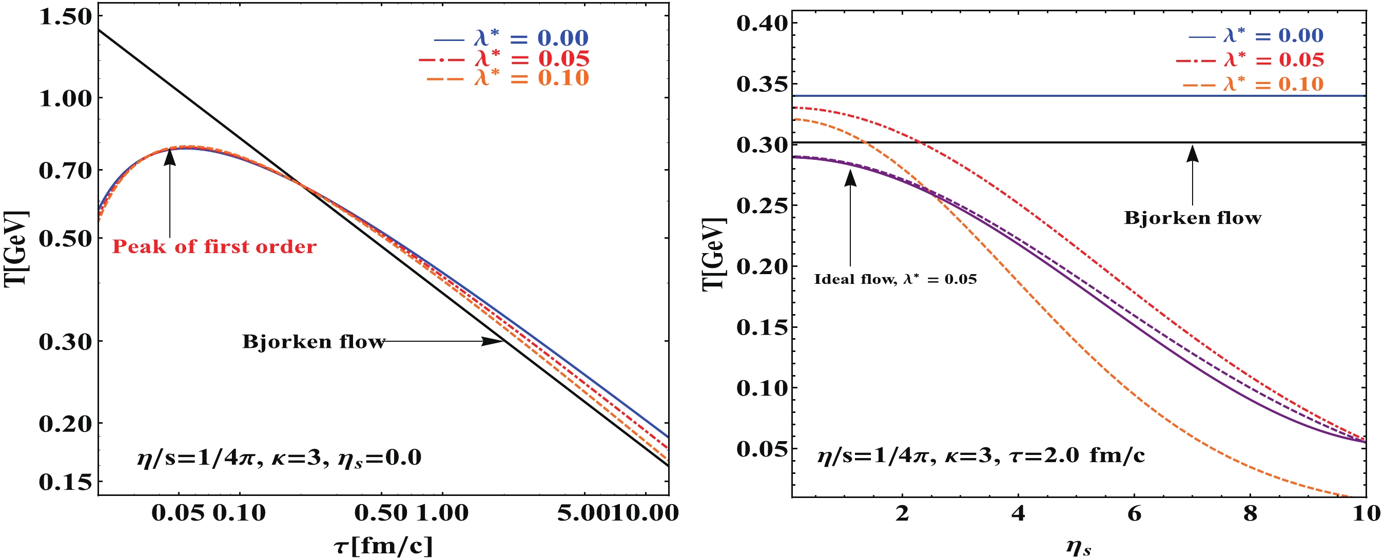
Figure 1. (color online) Temperature profile in the Navier-Stokes approximation for different longitudinal acceleration parameters
$ \lambda^{*} $ . Equation of state$ \varepsilon = 3p $ , shear viscosity ratio$ \eta/s = 1/4\pi $ . Black solid curve is the ideal Bjorken flow for reference, blue solid curve is the 1st order Bjorken flow. Left panel: The proper time$ \tau $ evolution with temperature for$ \eta_{s} = 0 $ . Right panel: space rapidity$ \eta_{s} $ evolution with temperature for$ \tau = 2 $ fm/c. Purple curve shows the comparison between the perturbation solution (dashed) and the numerical solution (solid) for ideal flow with$ \lambda^{*} = 0.05 $ , the accuracy is acceptable in the range$ 0.0\leqslant\eta_{s}\leqslant 5.0 $ . Results from the perturbation solution Eq. (24) and numerical solution for Eqs. (12), (13).The profile of Eq. (24) is a (1+1) dimensional scaling solution in (1+3) dimensions, and the
$ \eta_{s} $ dependence of temperature density is of the Gaussian form, see Fig. 1 right panel. Such perturbation solutions implies that for a non-vanishing longitudinal acceleration parameter$ \lambda^{*} $ , the cooling rate is larger than that for the ideal case. Meanwhile, a non-zero shear viscosity$ \eta $ makes the cooling rate smaller than the ideal case [38], see Fig. 1 left panel. Note that, when$ \lambda^{*} = 0 $ and$ R_{0}^{-1} = 0 $ , one obtains the same solutions as same as the ideal hydrodynamic Bjorken solution [13]; when$ \lambda^{*} = 0 $ and$ R_{0}^{-1}\neq0 $ , one obtains the first-order Bjorken solutions [7, 45]; if$ \lambda^{*}\neq0 $ and$ R_{0}^{-1} = 0 $ , one obtains a special solution which is consistent with the CNC solutions' case (e) in [16, 18], and when Eqs. (14), (15) are solved directly with$ R_{0}^{-1} = 0 $ and$ \lambda^{*}\neq0 $ , one obtains the CKCJ solutions [22].Case C. Perturbation equations with Israel-Stewart approximation.
The temperature profile from Eq. (24) shows a peak at earlier proper time
$ \tau $ in the Navier Stokes approximation, see Fig. 1. The source of this acausality can be understood from the constitutive relations satisfied by the dissipative currents$ \pi^{\mu\nu} = 2\eta\sigma^{\mu\nu} $ . The linear relationship between the dissipative currents and the gradients of the primary fluid-dynamical variables imply that any inhomogenity of$ u^{\mu} $ , immediately results in dissipative currents. This instantaneous effect causes the first-order theory to be unstable at earlier times.The Israel-Stewart (second-order) approximation was found to be suitable for describing the physical process happening at earlier times; it describes the counteract of the acceleration effect and viscosity effect well. However, it is difficult to solve the the differential equations Eqs. (12), (13) analytically with the Israel-Stewart approximation. Therefore, we numerically solve the temperature time dependence Eq. (12) first at
$ \eta_{s} = 0.0 $ with the initial condition$ T(0.2, 0.0) = 0.65 $ GeV; here the grid length of$ \tau $ is$ \Delta\tau = 0.05 $ fm. Then, for each$ \eta_{s} $ , we solve the temperature rapidity dependence Eq. (13) step by step with the results from the Eq. (12), and solve these equations together; the grid length of$ \tau $ is$ \Delta\tau = 0.05 $ fm. The temperature distribution of the thermodynamic quantities ($ \varepsilon,\; T,\; p $ ) in whole$ (\tau,\; \eta_{s}) $ coordinates with initial condition$ T(\tau_{0},\; \eta_{s0}) $ is a Gaussian shape, see Fig. 2. Furthermore, to compare with the perturbation results from the first-order approximation, Eqs. (12), (13) can be rewritten up to the leading order$ {\cal{O}}(\lambda^{*}) $ as follows,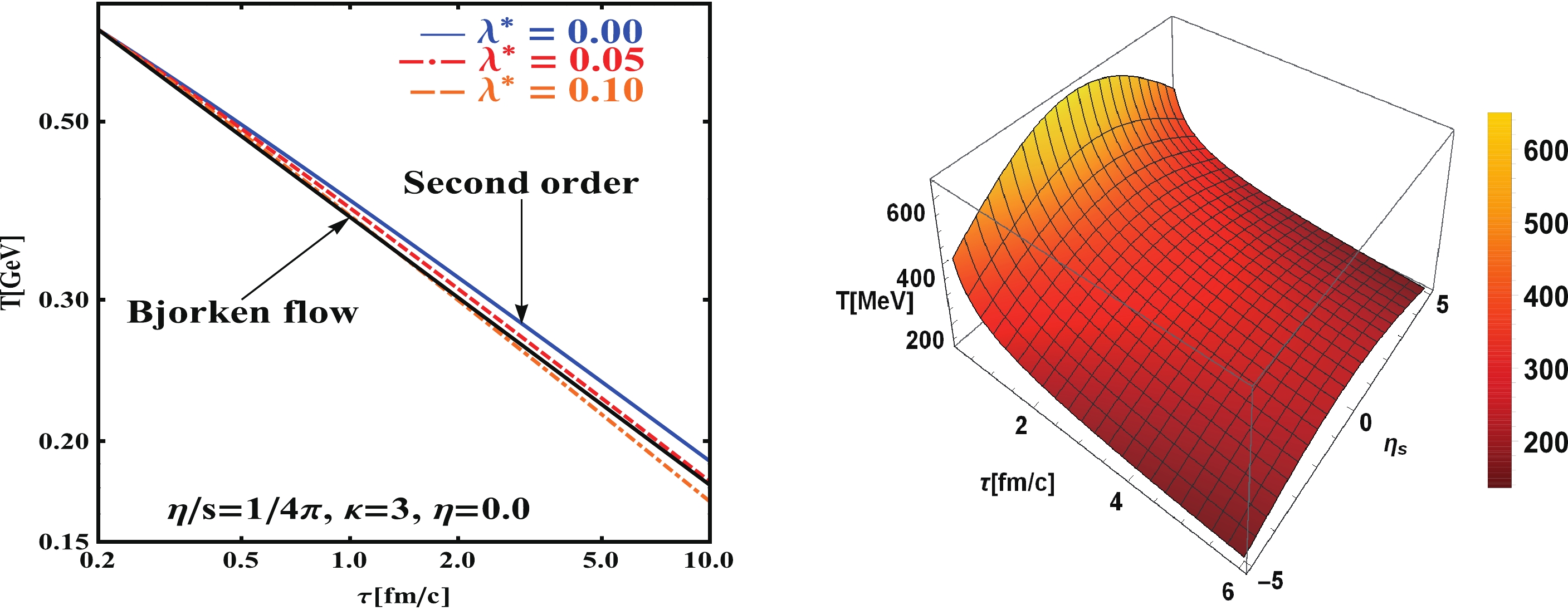
Figure 2. (color online) Temperature profile in the Israel-Stewart approximation. Left panel: proper time
$ \tau$ evolution of temperature for$ \eta_{s}=0$ . Black solid curve is the ideal Bjorken flow for reference. Right panel: The space-time evolution of temperature in ($ \tau-\eta_{s}$ ) coordinates, the longitudinal acceleration parameter$ \lambda^{*}=0.1$ . Numerical results from Eqs. (14), (15).$ \tau\frac{\partial T}{\partial\tau} = \frac{(2\lambda^{*}+1)\Pi_{d}}{3\tau}-\frac{(\lambda^{*}+1)T}{3}-\frac{(2-\ln 2)\Pi_{d}(1+6\lambda^{*})} {9 \pi T \tau^{2}}, $

(25) $ \frac{\partial T}{\partial\eta_{s}} = \lambda^{*}\eta_{s}\left[-\frac{2T}{3}-\frac{\Pi_{d}}{3\tau}+\frac{(2-\ln 2)\Pi_{d}}{9\pi T \tau^{2}} \right]. $

(26) The above differential equations (25), (26) cannot be solved analytically. Using the same numerical method as for the Eqs. (14), (15), we solve the above second-order viscous hydrodynamic equations (25), (26) with the conformal equation of state
$ \varepsilon\; = \; 3p $ and relaxation time$ \tau_{\pi} = \dfrac{2-\ln2}{2\pi T} $ [40-43] directly in the Rindler coordinates. The numerical results are presented in Fig. 3.
Figure 3. (color online) Proper time evolution of temperature density for given primary initial conditions. Left panel: Perturbation results of temperature profile in the Navier-Stokes approximation (1st) and in the Israel-Stewart theory (2nd). The longitudinal acceleration parameter
$ \lambda^{*}=0.10$ . Black solid curve is the ideal Bjorken flow for reference. Right panel: Temperature profile comparsion between the completely numerical solution (solid curve) with perturbation solutions (dashed curve) in the Israel-Stewart theory for different$ \lambda^{*}$ , the grid of$ \tau$ is$ \Delta\tau=0.05$ in the numerical code. -
The temperature profiles obtained in the previous section are now applied to study the longitudinal expanding dynamics, the initial condition
$ T(\tau_{0},\; \eta_{s0}) $ can be arbitrarily chosen. Following the result from [7], the initial proper time$ \tau_{0} = 0.2 $ fm/c, and initial temperature$ T_{0}(0.2,\; 0.0) = 0.65 $ GeV are used in the calculation.Figure 1 showed the longitudinal expanding effect dependence on temperature evolution in the Navier-Stokes approximation. Left panel of Fig. 1 showed the time-dependence of the temperature for different viscosity and the longitudinal acceleration parameter
$ \lambda^{*} $ . The black curve is the ideal Bjorken flow. It was seen that the larger the longitudinal acceleration parameter$ \lambda^{*} $ , the faster the medium cools down. However, the viscosity effect slow downs the medium cooling. It is important to note that there is a peak at early time in T in the case of first-order approximation. Right panel of Fig. 1showed the space-time rapidity dependence on the temperature at$ \tau = $ 2 fm/c. The temperature distribution of ideal Bjorken flow (black curve) and the Bjorken flow under Navier-Stokes limit (blue curve) show a flat-plateau shape. The effect of the longitudinally accelerating expansion, however, alters the temperature distribution to a Gaussian shape (red and orange curve). In addition, the difference between the numerical solution (purple solid curve) and the perturbation solution (purple dashed curve) for$ \Pi_{d} = \tau_{\pi} = 0 $ are presented. One finds that the difference in the range$ 0.0\leqslant\eta_{s}\leqslant 5.0 $ is acceptable.Figure 2 showed the complete temperature evolution for different longitudinal acceleration parameter
$ \lambda^{*} $ in the Israel-Stewart approximation. Left panel of Fig. 2 showed the time-dependence of the temperature. One finds no peak at the early time of T, the first-order theory significantly underpredicts the work done during the expansion relative to the Israel-Stewart approximation. One also finds that the effect of viscosity compensates the effect from longitudinal acceleration when$ \eta/s = 1/4\pi $ and$ \lambda^{*} = 0.05 $ ; at larger proper time of evolution, the viscous curve (red dashed) almost overlaps with the Bjorken flow (black solid). The longitudinal expansion effect make the medium cool down fast and there is no peak at early time in T. In the right panel of Fig. 2 shows the temperature distribution in ($ \tau,\eta_{s} $ ) coordinates with$ \lambda^{*} = 0.1 $ .Thus far, we focused on the study of the temperature evolution of perturbation solutions through the Navier-Stokes theories and Israel-Stewart theories independently. Now, we analyze the difference between these two theories under the same longitudinal acceleration effect. We numerically solve the differential equations Eqs. (25), (26) together with the initial condition
$ T_{0}(0.2,\; 0.0) = 0.65 $ GeV. The left panel of Fig. 3 showed the comparison of the second-order perturbation solutions, the first-order perturbation solutions and Bjorken solution. The right panel of Fig. 3 compares the second-order perturbation solutions and the completely numerical results. For small$ \lambda^{*} $ , we found that the perturbation solutions are stable and show good agreement with numerical results at large time. -
We have investigated the relativistic viscous hydrodynamics for longitudinally expanding fireballs in terms of the Navier-Stokes theory and Israel-Stewart theory by embedding 1+1 D fluid into a 1+3 D space-time. The results obtained in this paper are summarized as follows.
(1) We expand the current knowledge of accelerating hydrodynamics [16, 18, 22] by including the second-order viscous corrections in the relativistic hydrodynamics fluid with longitudinally expanding fireballs and general equation of state. The effect of longitudinal acceleration increases the thermodynamics evolution rate of the medium while the viscosity effect decelerates the evolution in the Minkowski space-time.
(2) The perturbation solution from the Navier-Stokes approximation is explicit and simple in mathematical structure, and it is consistent with the results from Ref. [38]. Furthermore, we compared the perturbation solution and the full numerical solution, which are presented in Fig. 1 right panel. It shows that the perturbation approximations for
$ \lambda\eta_{s} $ are valid in the leading order accuracy of the longitudinal acceleration parameter$ \lambda^{*} $ . The temperature distribution here indicates a Gaussian shape in the$ \eta_{s} $ direction.(3) For small perturbations along the longitudinal directions, as we presented in Fig. 1 right panel, the perturbation solution from the Navier-Stokes approximation is stable in the region with
$ \tau\geqslant \tau_{0} $ , while it is unstable in the region$ \tau\leqslant \tau_{0} $ .(4) The numerical results from the Israel-Stewart approximation in longitudinal expansion relativistic viscous hydrodynamics solve the causal problem and the temperature profile in the Rindler coordinate are presented.
There are still many open questions about such perturbation solutions and results.
(1) For consistency and stability, the perturbation solution is meaningful when
$ \lambda^{*} $ is pretty small and$ |\lambda^{*}\eta_{s}|\ll1 $ . For arbitrary longitudinal acceleration parameter$ \lambda^{*} $ , e.g.$ |\lambda^{*}|\gg 1 $ , such perturbation approximations become unsuitable and we need to solve the differential equations completely by other numerical method, such as 3+1D CLvisc [33]. In addition, if one treats the fluid rapidity$ \Omega $ as an unknown function of both the proper time$ \tau $ and space-time rapidity$ \eta_{s} $ , the conservation equations will be extremely complicated, compared with the current Eqs. (12), (13) even for the Navier-Stokes approximation, and the analytical solution will be difficult to arrive at (for more discussion about this issue, see [18]). (2) To find the new exact solutions of hydrodynamics, it is possible to use the method from the AdS/CFT theory [48, 49], which provides a method that searches the exact solutions by expanding in the small and large proper time$ \tau $ limit. (3) The shear pressure tensor relaxation time$ \tau_{\pi} $ assumed above for the second theory is definitely oversimplified, and it is only valid for smaller values of$ \tau_{\pi} $ . We acknowledge that this method is imperfect. (4) The transverse expansion cannot be neglected, especially during the later stages of the fireball, significantly changing the observables at RHIC and LHC. In reality, the expansion of the system will not be purely longitudinal, the system will also expand transversally [25, 28]. (5) It is important to note that the QGP bulk viscosity ratio$ \zeta/s $ is not zero from the lattice QCD calculation, the bulk viscosity plays a curial role when the temperature is greater than 3$ T_{c} $ [50, 51]. Recently, new solutions of first-order viscous hydrodynamics for Hubble-type flow are presented to study the bulk viscosity [52]; however, the second-order theory of such fluid is still unknown. (6) In principle, the second-order approximation should depend on a larger number of independent transport coefficient, e.g.$ \eta $ ,$ \tau_{\pi} $ ,$ \lambda_{1} $ ,$ \lambda_{2} $ ,$ \lambda_{3} $ , and, the direction extension results Eqs. (8), (9) from the$ \partial_{\mu}s^{\mu}\geqslant 0 $ are, in fact, incomplete and ad-hoc. To determine these transport coefficients, microscopic theories, such as kinetic theory should be studied [53]. (7) Chapman-Enskog expansion and completely Grid's 14-moment methods [54] could be used to study the higher order corrections. (8) Recently, the Duke group presented a novel method to study the effective viscosities [44], which points to a new way to study the shear viscosity and bulk viscosity for QGP. In the future, we plan to study the above aspects through more accurate studies in the future.We especially thank Xin-Nian Wang, M. Csanád, T. Csörgő, N. I. Nagy and Chao Wu for valuable comments at the initial stage of this study. Z-F. Jiang would like to thank T. Csörgő, M. Csanád, Lévai Péter and Gergely Gábor Barnafoldi for kind hospitality during his stay at Winger RCP, Budapest, Hungary.
Perturbation solutions of relativistic viscous hydrodynamics for longitudinally expanding fireballs
- Received Date: 2020-01-29
- Accepted Date: 2020-04-26
- Available Online: 2020-08-01
Abstract: The solutions of the relativistic viscous hydrodynamics for longitudinally expanding fireballs are investigated with the Navier-Stokes theory and Israel-Stewart theory. The energy and the Euler conservation equations for the viscous fluid are derived in Rindler coordinates, by assuming that the longitudinal expansion effect is small. Under the perturbation assumption, an analytical perturbation solution for the Navier-Stokes approximation and numerical solutions for the Israel-Stewart approximation are presented. The temperature evolution with both shear viscous effect and longitudinal acceleration effect in the longitudinal expanding framework are presented. The specific temperature profile shows symmetric Gaussian shape in the Rindler coordinates. Further, we compare the results from the Israel-Stewart approximation with the results from the Bjorken and the Navier-Stokes approximations, in the presence of the longitudinal acceleration expansion effect. We found that the Israel-Stewart approximation gives a good description of the early stage evolutions than the Navier-Stokes theory.


 DownLoad: