QCD corrections to ${{{e^+e^-}}{{\rightarrow}}{{H^{\pm}}}{{W^{\mp}}}}$ in Type-I THDM at electron positron colliders

In July 2012, the $125\; {\rm GeV}$ Higgs boson was discovered by ATLAS and CMS collaborations at the CERN Large Hadron Collider (LHC) [1, 2]. In addition to measuring the $125\; {\rm GeV}$ Higgs boson precisely, great efforts have been made to search for exotic Higgs bosons in various scenarios beyond the standard model (SM). Among all the extensions of the SM, the two-Higgs-doublet model (THDM) is an appealing one. It provides rich phenomena, such as charged Higgs bosons, explicit and spontaneous ${\cal CP}$-violation, and a candidate for dark matter, as the Higgs sector of the THDM is composed of two complex scalar doublets [3-6]. In THDM, there are five Higgs bosons: two neutral ${\cal CP}$-even Higgs bosons h and H ($m_h < m_H$), two charged Higgs bosons $H^{\pm}$ , and a neutral ${\cal CP}$-odd Higgs boson A. Although both ${\cal CP}$-even scalars can be interpreted as being the $125\; {\rm GeV}$ Higgs boson in the alignment limit, we assume that the lighter scalar h is the $125\; {\rm GeV}$ Higgs boson in this study. As flavor changing neutral currents (FCNCs) can be induced in THDM, which have not yet been observed, an additional $Z_2$ symmetry is imposed to eliminate FCNCs at the tree level. Depending on the types of the Yukawa interactions between fermions and the two Higgs doublets, one can introduce several different types of THDMs (Type-I, Type-II, lepton-specific, and flipped) [6]. The most investigated THDMs are Type-I and Type-II THDMs. For Type-I THDM, all fermions only couple to one of the two Higgs doublets, while for Type-II THDM, the up-type and down-type fermions couple to the two Higgs doublets respectively.

Many different aspects of THDMs have been widely studied in previous works. As it is possible to introduce a spontaneous ${\cal CP}$-violation in THDM, it has been considered as a solution to the problem of baryogenesis in Refs. [7-9]. In Refs. [10, 11], the neutral scalar in the inert THDM is interpreted as a candidate for dark matter. The existence of charged Higgs bosons $H^{\pm}$ is one important characteristic of new physics beyond the SM. Therefore, searching for a charged Higgs boson in various aspects is a high priority in experiments. At the LHC Run II, the charged Higgs boson has been probed in various channels, such as $H^{\pm} \rightarrow tb,\, \tau \nu_\tau\; \rm{and}\; WZ$ [12-15].

To match the precise experimental data, theoretical predictions on kinematic observables should be calculated with high precision. Renormalization of THDM has been studied in detail in different renormalization schemes in Refs. [16-20]. The production mechanisms and decay modes of the charged Higgs boson have been investigated at the one-loop level in THDM. The Drell-Yan production of charged Higgs pair has been studied at NLO in Refs. [21, 22]. The full one-loop contributions for the charged Higgs production associated with a vector boson are given in Refs. [22-25]. The dominant decays of the charged Higgs boson into tb and $\tau \nu_{\tau}$ have been studied in Refs. [26, 27], and the loop-induced decay modes $H^{\pm}\to W^{\pm}\gamma$ and $H^{\pm}\to W^{\pm}Z$ have also been investigated in Refs. [28-31]. In this work, we focus on $H^{\pm}W^{\mp}$ associated production at electron-positron colliders in Type-I THDM. This production channel is a loop-induced process at the lowest order due to the absence of tree-level $H^{\pm}W^{\mp}\gamma$ and $H^{\pm}W^{\mp}Z$ couplings, and has been investigated at one-loop level in THDM, as well as in the minimal supersymmetric standard model [32-35]. In order to test THDM via $H^{\pm}W^{\mp}V$ couplings precisely, we study in detail the two-loop QCD corrections to the $e^+e^- \rightarrow H^{\pm}W^{\mp}$ process, provide the NLO QCD corrected integrated and differential cross sections, and discuss the dependence on the THDM parameters and the $e^+e^-$ colliding energy.

The rest of this paper is organized as follows. In Sec. 2, we give a brief review of Type-I THDM and provide the benchmark scenario that we adopt. The methods and details of our LO and NLO calculations are presented in Sec. 3. In Sec. 4, the numerical results for both integrated and differential cross sections and some discussions are provided. Finally, a short summary is given in Sec. 5.

The Higgs sector of THDM is composed of two complex scalar doublets, $\Phi_1 = (\phi_{1}^{+},\phi_{1}^0)^{T}$ and $\Phi_2 = (\phi_{2}^{+},\phi_{2}^0)^{T}$, which are both in the $(\mathbf{1}, \mathbf{2}, \mathbf{1})$ representation of the $SU(3)_C \otimes SU(2)_L \otimes U(1)_Y$ gauge group. In this paper, we consider only the ${\cal CP}$-conserving THDM with a discrete $Z_2$ symmetry of the form $\Phi_1 \rightarrow -\Phi_1$. Then, the renormalizable and gauge invariant scalar potential is given by

As parameter $m_{12}$ has mass-dimension 1, terms of this type only break the $Z_2$ symmetry softly, which can therefore be retained. The parameters $m_{11},\, m_{22},\, \lambda_{1},\, \lambda_{2},\, \lambda_{3},\, \lambda_{4}$ have to be real, as the Lagrangian must be real. Though parameters $m_{12}$ and $\lambda_{5}$ can be complex, the imaginary parts of these two parameters would induce explicit ${\cal CP}$ violation that we do not consider in this paper. So, we assume all parameters in Eq. (1) are real. The minimization of the potential in Eq. (1) gives two minima, $\langle\Phi_{1}\rangle$ and $\langle\Phi_{2}\rangle$, of the form

where $v_{1}$ and $v_{2}$ are the vacuum expectation values of the neutral components of the two Higgs doublets $\Phi_{1}$ and $\Phi_{2}$, respectively. With respect to the convention in Ref. [36], we define $v_1 = v\cos\beta$ and $v_2 = v\sin\beta$, where $v = (\sqrt{2}G_{F})^{-1/2} \approx246\; {\rm GeV}$. Expanding at the minima, the two complex Higgs doublets $\Phi_{1,2}$ can be expressed as

The mass eigenstates of the Higgs fields are given by [6, 20]

where $\alpha$ is the mixing angle of the neutral ${\cal CP}$-even Higgs sector. After the spontaneous electroweak symmetry breaking, the charged and neutral Goldstone fields $G^{\pm}$ and $G^{0}$ are absorbed by the weak gauge bosons $W^{\pm}$ and Z, respectively. Thus, THDM predicts the existence of five physical Higgs bosons: two neutral ${\cal CP}$-even Higgs bosons h and H, one neutral ${\cal CP}$-odd Higgs boson A, and two charged Higgs bosons $H^{\pm}$. The masses of these physical Higgs bosons are given by

where ${\cal M}^2$ is the mass matrix of the neutral ${\cal CP}$-even Higgs sector. The explicit form of ${\cal M}^2$ is expressed as

where

SM Higgs is the combination of the two neutral ${\cal CP}$-even Higgs bosons as

Thus, the lighter neutral ${\cal CP}$-even scalar h can be identified as the SM-like Higgs boson in the so-called alignment limit of $\sin(\beta-\alpha)\rightarrow 1$. In this paper, we consider the lighter ${\cal CP}$-even Higgs h as being the SM-like Higgs boson discovered at the LHC.

The input parameters for the Higgs sector of the THDM are chosen as

which are implemented as the “physical basis” in 2HDMC [36]. We adopt the following benchmark scenario,

which satisfies the theoretical constraints from perturbative unitarity [37], stability of vacuum [38], and tree-level unitarity [39]. The $Z_{2}$ soft-breaking parameter $m_{12}^2$ is chosen as $m_{A}^{2}\sin\beta\cos\beta$ in order to satisfy the perturbative unitarity for $\tan\beta \in [1, 5]$. Considering the constraints from the experiments at the $13\; {\rm TeV}$ LHC in Ref. [40], $\cos(\beta-\alpha)$ is very close to 0. So, we apply the alignment limit in our benchmark scenario to set $\sin(\beta-\alpha) = 1$. Regarding the $m_{H^{\pm}}$ and $\tan\beta$ parameters, we concentrate on the region with low mass and small $\tan\beta$.

In this section, we present in detail the calculation procedure for the $e^{+}e^{-}\rightarrow H^{\pm}W^{\mp}$ process at one- and two-loop levels. The Feynman diagrams and the amplitudes are generated by FeynArts-3.11 [41] using the Feynman rules of THDM in Ref. [20]. The evaluation of the Dirac trace and the contraction of the Lorentz indices are performed by the FeynCalc-9.3 package [42, 43]. In order to reduce the Feynman integrals into combinations of a small set of integrals called the master integrals (MIs), we utilize the KIRA-1.2 package [44], which adopts the integration-by-parts (IBP) method with Laporta's algorithm [45]. One can determine the numerical results of amplitudes after evaluating the MIs, which is the main difficulty encountered in multi-loop calculation.

In this study, we calculate the MIs by using the ordinary differential equations (ODEs) method [46]. A L-loop Feynman integral can be expressed as

where $D\equiv 4-2\epsilon$ and $E_{k} = q_{k}^{2}-m_{k}^2$ are the denominators of Feynman propagators, in which $q_{k}$ are the linear combinations of loop momenta and external momenta. The physical results of the Feynman integrals are obtained by taking $\eta \rightarrow 0^+$, i.e.,

One can construct the ODEs with respect to $\eta$,

where $\vec{{\cal I}}$ is a complete set of MIs. The boundary conditions of these ODEs are chosen to be at $\eta = \infty$, which are the simple vacuum integrals. The analytical expressions for the vacuum integrals up to three-loop order can be found in Refs. [47-49]. To solve these ODEs numerically, we utilize the odeint package [50] for evaluating ODEs from an initial point $\eta_i$ to a target point $\eta_j$. To perform the asymptotic expansion in the domain close to $\eta = 0$, we transform the coefficient matrix into the normalized fuchsian form with the help of the epsilon package [51].

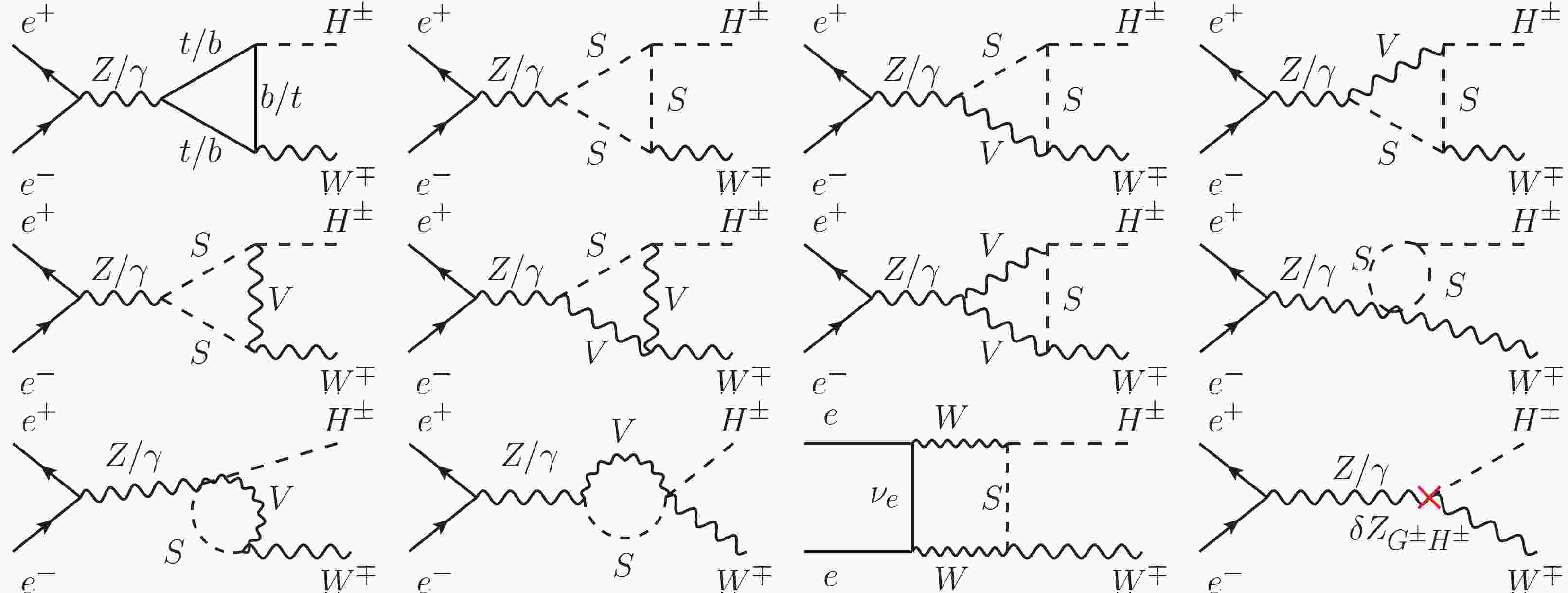
For the LO calculation, we adopt the 't Hooft-Feynman gauge with the on-shell renormalization scheme at one-loop order mentioned in Ref. [20]. Some representative Feynman diagrams for the $e^{+}e^{-} \rightarrow H^{\pm}W^{\mp}$ process at the LO are shown in Fig. 1, where S and V in the loops represent the Higgs/Goldstone and weak gauge bosons, respectively. Due to the tiny mass of the electron, the contributions from the diagrams involving Higgs Yukawa coupling to electron are ignored. The diagrams with $V-S$ mixing are also not shown in Fig. 1, because these diagrams can induce a factor of $m_e$ via the Dirac equation. The last diagram in Fig. 1 is a vertex counterterm diagram induced by the renormalization constant $\delta Z_{G^{\pm}H^{\pm}}$ at one-loop level. In the on-shell renormalization scheme, the renormalization constant $\delta Z_{G^{\pm}H^{\pm}}$ is given by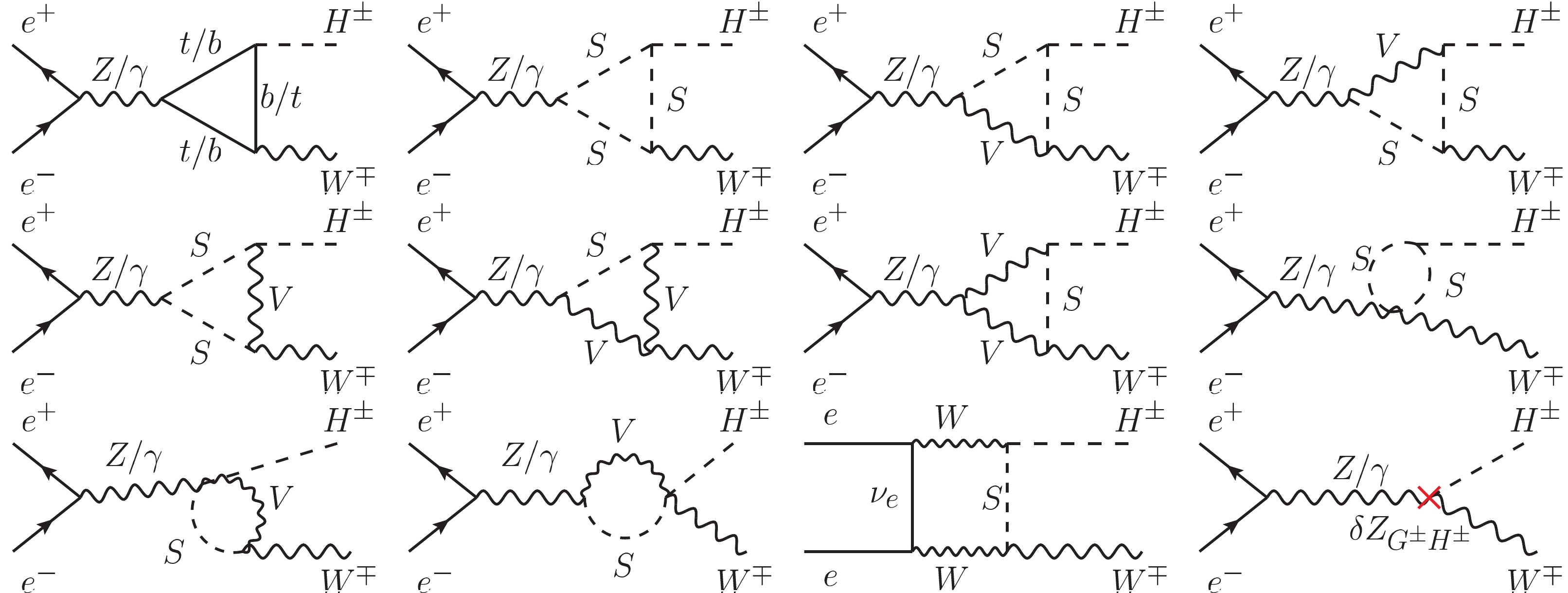

Figure 1.  Representative Feynman diagrams for $e^{+}e^{-} \rightarrow H^{\pm}W^{\mp}$ at LO.

where $\sum^{W^{\pm}H^{\pm}}(m_{H^{\pm}}^2)$ is the transition of $W^{\pm}-H^{\pm}$ at $p^{2} = m_{H^{\pm}}^2$, and $\widetilde{Re}$ means to take the real parts of the loop integrals in the transition. It is worth mentioning that Eq. (16) is valid at both, ${\cal O}(\alpha)$ and ${\cal O}(\alpha\alpha_s)$.

There are 24 two-loop and counterterm diagrams for $e^{+}e^{-} \rightarrow H^{\pm}W^{\mp}$ at the QCD NLO. Some representative ones are depicted in Fig. 2. At the QCD NLO, all two-loop Feynman diagrams are generated from the LO quark triangle loop diagram (i.e., the first diagram in Fig. 1). The cross in the quark loop diagrams represents the renormalization constant of the quark mass at ${\cal O}(\alpha_{s})$, while the circle cross displayed in the last counterterm diagram represents the renormalization constant $\delta Z_{G^{\pm}H^{\pm}}$ at ${\cal O}(\alpha\alpha_{s})$. The quark mass renormalization constant used in the NLO QCD calculation is given by [52]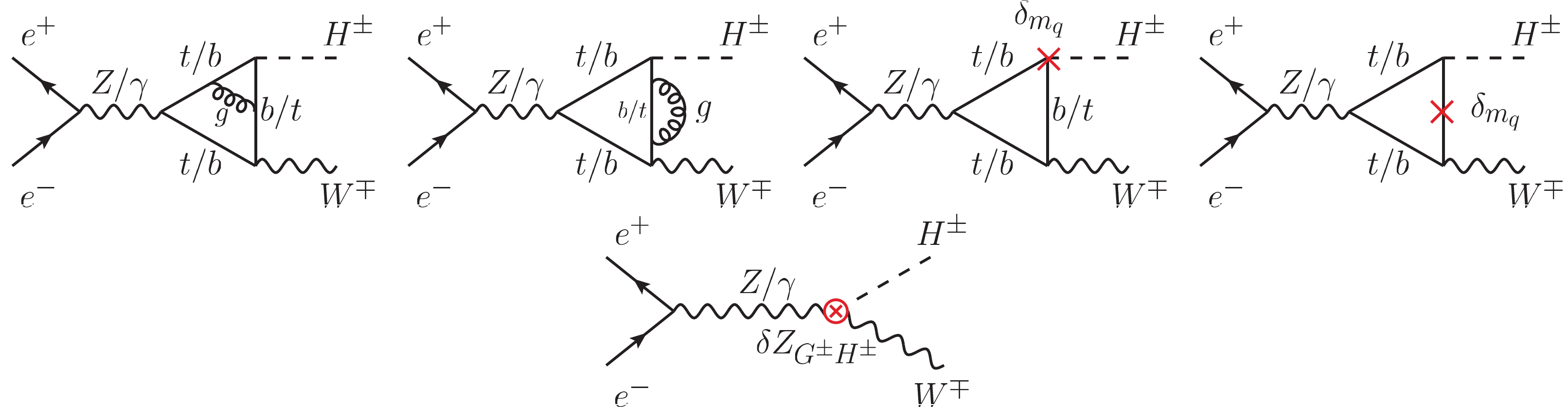

Figure 2.  (color online) Representative Feynman diagrams for $e^{+}e^{-} \rightarrow H^{\pm}W^{\mp}$ at NLO in QCD.

where $C(\epsilon) = (4\pi)^{\epsilon}\Gamma(1+\epsilon)$ and $C_{F} = \dfrac{4}{3}$. The lowest order for $e^{+}e^{-} \rightarrow H^{\pm}W^{\mp}$ is the one-loop order, therefore, renormalization should be dealt with carefully in NLO QCD calculation. As shown in Figs. 1 and 2, the wave-function renormalization constant $\delta Z_{G^{\pm}H^{\pm}}$ is involved in both NLO and LO amplitudes. As the self-energy $\sum^{W^{\pm}H^{\pm}}(m_{H^{\pm}}^2)$ is non-zero at ${\cal O}(\alpha\alpha_{s})$, i.e. $\delta Z_{G^{\pm}H^{\pm}}$ is non-zero at ${\cal O}(\alpha\alpha_{s})$, the contribution from the last diagram in Fig. 2 should be included in the NLO QCD calculation. Typical Feynman diagrams for the $H^{\pm}-W^{\pm}$ transition at ${\cal O}(\alpha\alpha_{s})$ are shown in Fig. 3. After taking into account all contributions at ${\cal O}(\alpha\alpha_{s})$ in D-dimensional spacetime, both, $\dfrac{1}{\epsilon^2}$ and $\dfrac{1}{\epsilon}$ singularities are all canceled.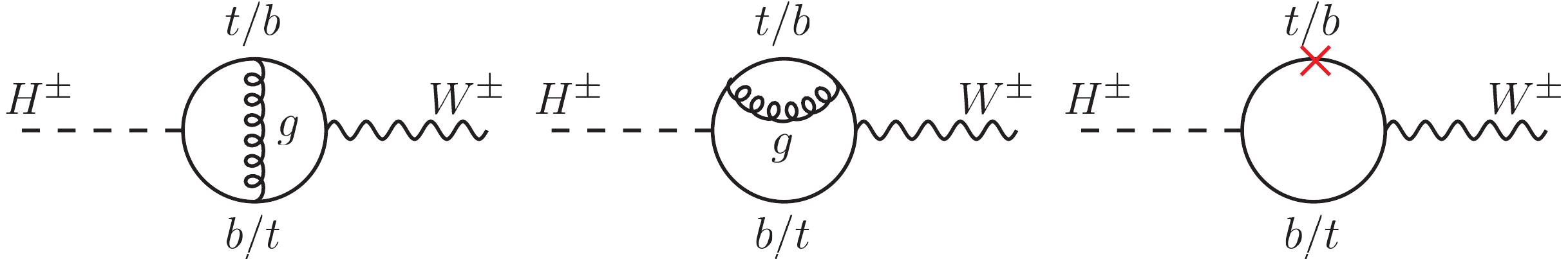

Figure 3.  (color online) Representative Feynman diagrams contributing to $W^{\pm}-H^{\pm}$ transition at ${\cal O}(\alpha\alpha_{s})$.

Besides the input parameters for the Higgs sector of the THDM specified in benchmark scenario in Eq. (12), the following SM input parameters are adopted in our numerical calculation [53]:

where $G_{F}$ is the Fermi constant. The fine structure constant $\alpha$ is fixed by

In Fig. 4, we display the LO cross section for $e^{+}e^{-} \rightarrow H^{\pm}W^{\mp}$ as a function of $m_{H^{\pm}}$ and $\tan\beta$ in the benchmark scenario in Eq. (12) at $\sqrt{s} = 500\; {\rm GeV}$ (left) and $1000\; {\rm GeV}$ (right). From the left plot, we can see clearly that the LO cross section for $H^{\pm}W^{\mp}$ production at a $500\; {\rm GeV}$ $e^+e^-$ collider peaks at $m_{H^{\pm}} \simeq 184\; {\rm GeV}$ due to the resonance effect of loop integrals. The cross section is sensitive to the mass of the charged Higgs boson, it can exceed $3\; {\rm fb}$ in the vicinity of $m_{H^{\pm}} \simeq 184\; {\rm GeV}$ at small $\tan\beta$. In the region of $m_{H^{\pm}}<180\; {\rm GeV}$, the cross section increases slowly with the increase of $m_{H^{\pm}}$, while it drops rapidly when $m_{H^{\pm}} > 184\; {\rm GeV}$. When $\tan\beta$ increases from 1 to 5, the cross section decreases consistently due to the decline of the $H^{+}\bar{t}b$ Yukawa coupling strength in the low $\tan\beta$ region. Comparing the two plots in Fig. 4, we can see that the cross section at $\sqrt{s} = 1000\; {\rm GeV}$ is much smaller than that at $\sqrt{s} = 500\; {\rm GeV}$ because of s-channel suppression. As the $e^+e^-$ colliding energy increases from 500 to $1000\; {\rm GeV}$, the peak position of the cross section as a function of $m_{H^{\pm}}$ moves towards high $m_{H^{\pm}}$ and the $m_{H^{\pm}}$ dependence of the cross section is reduced significantly. Moreover, the production cross section at $\sqrt{s} = 1000\; {\rm GeV}$ also decreases quickly with the increase of $\tan\beta$ in the plotted $\tan\beta$ region.

Figure 4.  (color online) Contours of LO cross section for $e^{+}e^{-} \rightarrow H^{\pm}W^{\mp}$ at $\sqrt{s} = 500\; {\rm GeV}$ (left) and $1000\; {\rm GeV}$ (right) on the $m_{H^{\pm}}-\tan\beta$ plane.

In Fig. 5, we present the dependence of the LO cross section for $e^+e^- \rightarrow H^{\pm}W^{\mp}$ on the $e^+e^-$ colliding energy for some typical values of $m_{H^{\pm}}$ and $\tan\beta$. As shown in this figure, the behaviors of the production cross section as a function of the colliding energy at different values of $\tan\beta$ are quite similar. For $m_{H^{\pm}} = 160\; {\rm GeV}$, the cross section increases sharply in the range of $\sqrt{s} < 360\; {\rm GeV}$, reaches its maximum at $\sqrt{s} \simeq 360\; {\rm GeV}$, and then decreases slowly with the increase of $\sqrt{s}$. The existence of the peak at $\sqrt{s} \simeq 360\; {\rm GeV}$ can be attributed to the competition between the phase-space enlargement and the s-channel suppression with the increase of $\sqrt{s}$. The maximum value of the cross section can exceed $1\; {\rm fb}$ for $\tan\beta = 1$ and decreases to about $0.3\; {\rm fb}$ and $0.1\; {\rm fb}$ for $\tan\beta = 2$ and $\tan\beta = 3$, respectively. Comparing the upper two plots of Fig. 5, we can see that the $\sqrt{s}$ dependence of the cross section for $m_{H^{\pm}} = 180\; {\rm GeV}$ is very close to that for $m_{H^{\pm}} = 160\; {\rm GeV}$, but there is a small peak at $\sqrt{s} \simeq 630\; {\rm GeV}$ for $m_{H^{\pm}} = 180\; {\rm GeV}$. Such resonance induced by loop integrals only occurs above the threshold of $H^{+} \rightarrow t \bar{b}$, i.e., $m_{H^{\pm}} > m_t + m_b$. With the increase of $m_{H^{\pm}}$, this resonance effect becomes more considerable and the peak position moves towards low $\sqrt{s}$. As shown in the bottom-left plot of Fig. 5, the resonance peak for $m_{H^{\pm}} = 185\; {\rm GeV}$ is located at $\sqrt{s} \simeq 490\; {\rm GeV}$, and is more distinct compared with that for $m_{H^{\pm}} = 180\; {\rm GeV}$. Regarding the $\sqrt{s}$ dependence of the $H^{\pm}W^{\mp}$ production cross section for $m_{H^{\pm}} = 200\; {\rm GeV}$ shown in the bottom-right plot of Fig. 5, it looks quite different from those for $m_{H^{\pm}} = 160,\, 180$ and $185\; {\rm GeV}$. There is a sharp peak at $\sqrt{s} \simeq 390\; {\rm GeV}$ for each value of $\tan\beta \in \{1, 2, 3\}$, which was also mentioned in previous works [22, 23, 25]. This peak is a consequence of competition among the phase-space enlargement, s-channel suppression and the resonance induced by loop integrals. We can see that the peak cross section can reach about $4\; {\rm fb}$ for $\tan\beta = 1$, and will decrease to around $1\; {\rm fb}$ and $0.4\; {\rm fb}$ when $\tan\beta$ increases to 2 and 3, respectively. In the region of $\sqrt{s} < 350\; {\rm GeV}$, the cross section increases quickly with the increase of $\sqrt{s}$ due to the enlargement of phase space, while in the region $\sqrt{s} > 450\; {\rm GeV}$, it is close to the result of s-channel suppression, especially at high $\sqrt{s}$.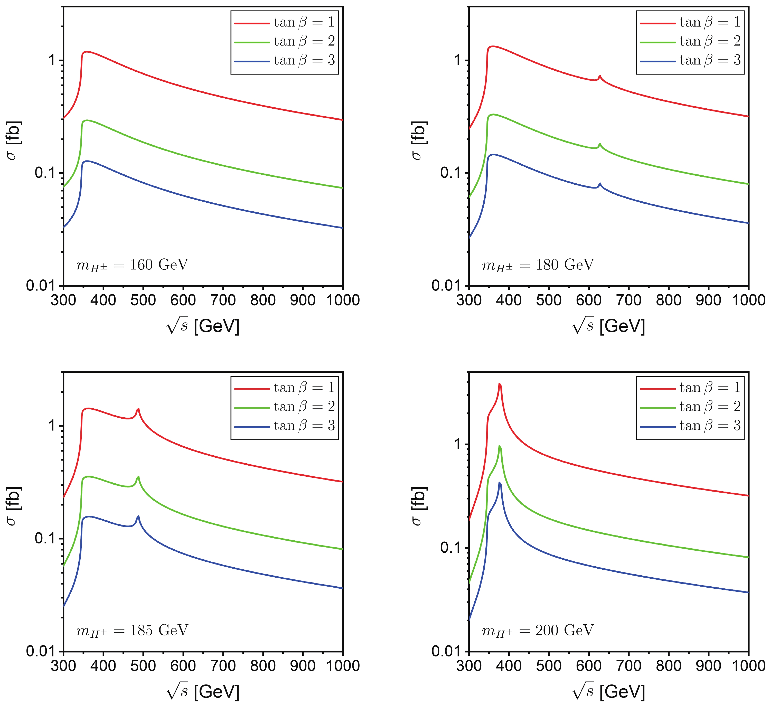

Figure 5.  (color online) LO cross section for $e^{+}e^{-} \rightarrow H^{\pm}W^{\mp}$ as a function of $e^+e^-$ colliding energy for some typical values of $m_{H^{\pm}}$ and $\tan\beta$.

In this subsection, we calculate the $e^+e^- \rightarrow H^{\pm}W^{\mp}$ process at the QCD NLO, and discuss the dependence of the integrated cross section on the $e^+e^-$ colliding energy and the charged Higgs mass, as well as the angular distribution of the final-state charged Higgs boson.

The LO, NLO QCD corrected integrated cross sections and the corresponding QCD relative correction for $e^+e^- \rightarrow H^{\pm}W^{\mp}$ as functions of the $e^+e^-$ colliding energy $\sqrt{s}$ are depicted in Fig. 6, where $m_{H^{\pm}} = 200\; {\rm GeV}$ and $\tan\beta = 2$. As shown in the upper panel of this figure, the NLO QCD corrected integrated cross section peaks at $\sqrt{s} \simeq 375\; {\rm GeV}$. It increases sharply for$\sqrt{s} < 375\; {\rm GeV}$ and decreases approximately linearly in the region of $\sqrt{s} > 500\; {\rm GeV}$ with the increase of $\sqrt{s}$. From the lower panel of Fig. 6, we can see that the QCD relative correction increases rapidly from about 9% to above 60% with the increment of $\sqrt{s}$ from 300 to $345\; {\rm GeV}$ and then decreases back to about 3% as $\sqrt{s}$ increases to $385\; {\rm GeV}$. The variation of the QCD relative correction with $\sqrt{s}$ in the region of $\sqrt{s} > 385\; {\rm GeV}$ is also plotted in the inset in the upper panel of Fig. 6 for clarity. It clearly shows that the QCD relative correction decreases approximately linearly from about 3% to around -4% with the increment of $\sqrt{s}$ from 385 to $1000\; {\rm GeV}$. In Table 1, we list the LO, NLO QCD corrected cross sections and the corresponding QCD relative corrections at some specific colliding energies. At $\sqrt{s} = 340\; {\rm GeV}$, which can be reached by both the International Linear Collider (ILC) [54] and the Future Circular Electron-Positron Collider (FCC-ee) [55], the cross section is about $0.235\; {\rm fb}$ at the QCD NLO. At the ILC with $\sqrt{s} = 500$ and $1000\; {\rm GeV}$, the NLO QCD corrected cross sections reach about 0.193 and $0.0778\; {\rm fb}$, respectively, and the corresponding relative corrections are 0.26% and −4.27%.

$\sqrt{s}$/GeV	300	320	340	400	500	600	700	800	900	1000
$\sigma_{ \rm{LO}}$/fb	0.04592	0.07868	0.1712	0.3870	0.1920	0.1481	0.1230	0.1054	0.09196	0.08126
$\sigma_{ \rm{NLO}}$/fb	0.05004	0.09163	0.2353	0.3963	0.1925	0.1466	0.1206	0.1024	0.08865	0.07779
$\delta$(%)	8.97	16.4	37.4	2.40	0.260	−1.01	−1.95	−2.85	−3.60	−4.27

Table 1.  LO, NLO QCD corrected cross sections and the corresponding QCD relative corrections for $e^+e^- \rightarrow H^{\pm}W^{\mp}$ at some specific colliding energies. ($m_{H^{\pm}} = 200\; {\rm GeV}$ and $\tan\beta = 2$).

Figure 6.  (color online) LO, NLO QCD corrected integrated cross sections and the corresponding QCD relative correction for $e^+e^- \rightarrow H^{\pm}W^{\mp}$ as functions of $e^+e^-$ colliding energy for $m_{H^{\pm}} = 200\; {\rm GeV}$ and $\tan\beta = 2$.

In order to study the $m_{H^{\pm}}$ dependence of the QCD correction, we plot the NLO QCD corrected cross section, as well as the LO cross section, and the QCD relative correction as functions of $m_{H^{\pm}}$ in Fig. 7 with $\tan\beta = 2$ and $\sqrt{s} = 500\; {\rm GeV}$. The numerical results for some typical values of $m_{H^{\pm}}$ are also given in Table 2. From Fig. 7, we can see that the LO and NLO QCD corrected cross sections increase from about $0.18\; {\rm fb}$ to around 0.29 and $0.32\; {\rm fb}$, respectively, as $m_{H^{\pm}}$ increases from 150 to $184\; {\rm GeV}$, and drop to less than $0.01\; {\rm fb}$ for $m_{H^{\pm}} = 400\; {\rm GeV}$. Similarly, there is also a notable spike at $m_{H^{\pm}} \simeq 184\; {\rm GeV}$ in the QCD relative correction, as shown in the lower panel of Fig. 7. The QCD relative correction is less than 0.5% and thus, can be neglected for $m_{H^{\pm}} = 150\; {\rm GeV}$, while it is expected to increase to about 11% as $m_{H^{\pm}}$ increases to $184\; {\rm GeV}$. When $m_{H^{\pm}} > 185\; {\rm GeV}$, the QCD relative correction decreases slowly to about -10% as $m_{H^{\pm}}$ increases to $400\; {\rm GeV}$.

$m_{H^{\pm}}$/GeV	150	160	170	180	190	200	250	300	350	400
$\sigma_{ \rm{LO}}$/fb	0.1828	0.1876	0.1951	0.2140	0.2230	0.1920	0.1090	0.05699	0.02553	0.007595
$\sigma_{ \rm{NLO}}$/fb	0.1836	0.1896	0.1990	0.2249	0.2240	0.1925	0.1062	0.05376	0.02343	0.006817
$\delta$(%)	0.438	1.07	2.00	5.09	0.448	0.260	−2.57	−5.67	−8.22	−10.24

Table 2.  LO, NLO QCD corrected cross sections and the corresponding QCD relative corrections for $H^{\pm}W^{\mp}$ production at a $\sqrt{s} = 500\; {\rm GeV}$ $e^+e^-$ collider for some typical values of $m_{H^{\pm}}$. ($\tan\beta = 2$).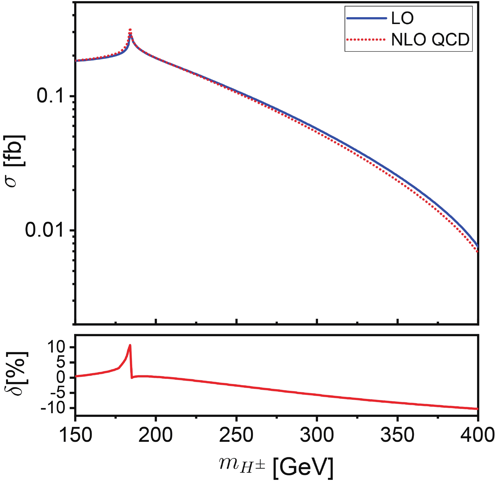

Figure 7.  (color online) LO, NLO QCD corrected cross sections and the corresponding QCD relative correction for $H^{\pm}W^{\mp}$ associated production at a $\sqrt{s} = 500\; {\rm GeV}$ $e^+e^-$ collider as functions of charged Higgs mass for $\tan\beta = 2$.

The LO, NLO QCD corrected angular distributions of the final-state charged Higgs boson and the corresponding QCD relative corrections for $H^+W^-$ associated production at a $500\; {\rm GeV}$ $e^+e^-$ collider for $\tan\beta = 2$ and $m_{H^{\pm}} = 200$ and $300\; {\rm GeV}$ are depicted in Fig. 8, where $\theta$ denotes the scattering angle of $H^+$ with respect to the electron beam direction. Due to ${\cal CP}$ conservation, the distribution of the scattering angle of $H^-$ with respect to the positron beam direction for $e^+e^- \rightarrow H^-W^+$ is the same as the angular distribution of $H^+$ for $e^+e^- \rightarrow H^+W^-$. From this figure, we can see that the charged Higgs boson is mostly produced in the transverse direction for $m_{H^{\pm}} = 200$ and $300\; {\rm GeV}$. For $m_{H^{+}} = 200\; {\rm GeV}$, the QCD relative correction decreases rapidly from 10% to nearly 0% with the increment of $\cos\theta$ from -1 to -0.5, and is steady at around 0% in the region of $-0.5 < \cos\theta < 1$. It implies that the NLO QCD correction can be neglected in most of the phase space region, except when $\theta \rightarrow \pi$. For $m_{H^{\pm}} = 300\; {\rm GeV}$, the LO differential cross section is suppressed by the NLO QCD correction in the whole phase space region. The corresponding QCD relative correction decreases from about -0.8% to -7.5% as $\cos\theta$ increases from -1 to 1. This QCD correction should be taken into consideration in a precision study of the $H^{\pm}W^{\mp}$ production at lepton colliders.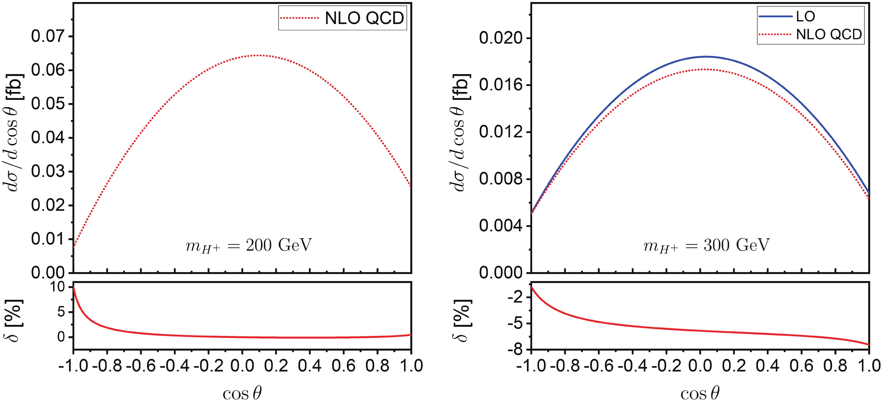

Figure 8.  (color online) Angular distributions of charged Higgs boson for $H^+W^-$ associated production at a $500\; {\rm GeV}$ $e^+e^-$ collider for $\tan\beta = 2$ and $m_{H^{\pm}} = 200$ (left) and $300\; {\rm GeV}$ (right).

Searching for exotic Higgs bosons and studying its properties are important tasks for future lepton colliders. In this work, we study in detail the $H^{\pm}W^{\mp}$ associated production at future electron-positron colliders within the framework of Type-I THDM. We calculate the $e^+e^- \rightarrow H^{\pm}W^{\mp}$ process at the LO and investigate the dependence of the production cross section on the THDM parameters ($m_{H^{\pm}}$ and $\tan\beta$) and the $e^+e^-$ colliding energy. The numerical results show that the cross section is very sensitive to the charged Higgs mass in the vicinity of $m_{H^{\pm}} \simeq 184\; {\rm GeV}$ at a $500\; {\rm GeV}$ $e^+e^-$ collider, and it decreases consistently with the increase of $\tan\beta$ in the low $\tan\beta$ region. The existence of a peak in the colliding energy distribution of the cross section is explained by the resonance effect induced by loop integrals. This resonance occurs only above the threshold of $H^+ \rightarrow t \bar{b}$, and the peak position moves towards the low colliding energy with the increase of $m_{H^{\pm}}$. We also calculate two-loop NLO QCD corrections to $e^+e^- \rightarrow H^{\pm}W^{\mp}$ and provide some numerical results for the NLO QCD corrected integrated cross section and the angular distribution of the final-state charged Higgs boson. For $\sqrt{s} = 500\; {\rm GeV}$ and $\tan\beta = 2$, the QCD relative correction varies smoothly in the range of [-10%, 3%] with the increase of $m_{H^{\pm}}$ from $150$ to $400\; {\rm GeV}$, except in the vicinity of $m_{H^{\pm}} \simeq 184\; {\rm GeV}$. The QCD relative correction is sensitive to the charged Higgs mass and strongly depends on the final-state phase space. For $m_{H^{\pm}} = 300\; {\rm GeV}$ and $\tan\beta = 2$, the QCD relative correction to the $H^+W^-$ production at a $500\; {\rm GeV}$ $e^+e^-$ collider increases from about -7.5% to -0.8% as the scattering angle of $H^+$ increases from 0 to $\pi$. Compared to hadron colliders, the measurement precision of Higgs associated production at future high-energy electron-positron colliders is much higher. The expected experimental error of Higgs production in association with a weak gauge boson at high-energy electron-positron colliders is less than 1% through the recoil mass of the associated vector boson. For example, the measurement precision of $HZ$ production at $\sqrt{s} = 240\; {\rm GeV}$ FCC-ee and $\sqrt{s} = 250\; {\rm GeV}$ CEPC can reach about 0.4% and 0.7%, respectively [56-58]. Due to the high $W$-tagging efficiency at $e^+e^-$ colliders, the measurement precision of $H^{\pm}W^{\mp}$ production at a high-energy $e^+e^-$ collider can be also less than 1%. Thus, two-loop QCD correction should be taken into consideration in precision studies of $H^{\pm}W^{\mp}$ associated production at future lepton colliders.