


 Abstract
 HTML
HTML Reference
 Related
 PDF
PDF


-
In 2012, the Higgs boson predicted by the standard model (SM) was discovered by the LHC, launching a new era in particle physics [1]. Although the SM has been very successful, many issues have yet to be resolved, including the hierarchy problem and the absence of dark matter particles. In the SM, the mass of the Higgs boson requires quadratic corrections to the energy scale
$\Lambda$ . It is difficult to explain that the mass of the Higgs boson is on the electroweak scale, if$\Lambda$ is set to the Planck or Grand Unified Theory (GUT) scale. This is the hierarchy problem. Therefore, above the electroweak scale, new interactions, symmetries, and particles could emerge and provide a natural solution to the hierarchy problem. Although the neutrinos in the SM have the properties of dark matter, they do not fully explain astronomical and cosmological observations. Therefore, to say the least, new physics may contain new particles that could be candidates for dark matter. Based on the above two observations, it can be inferred that new physics contains a new mechanism to solve the hierarchy problem and to introduce new particles. The supersymmetry theory, introducing the symmetry of bosons and fermions, is one of the solutions to these problems. It solves the hierarchy problem and contains possible candidates for dark matter particles. In addition, if the Higgs boson is considered a composite particle, that is, dynamical electroweak symmetry breaking is introduced, the above problems can also be solved.As the Higgs boson is an elementary scalar particle in the SM, its radiation correction requires significant fine-tuning. As is well known, further spontaneous symmetry breaking in nature comes from the condensation of composite operators. Therefore, one solution is tantamount to treating the Higgs boson as a composite particle derived from the new strongly coupled technicolor condensation. Therefore, the electroweak part of the SM is the effective field theory, and when the energy scale reaches
$ \Lambda_{TC} $ , the details of the new interaction will be revealed. The SM does not explain the origin of the spontaneous electroweak symmetry breaking, and technicolor as an alternative idea can avoid the hierarchy problem without introducing an elementary scalar field. Technicolor is a new strongly coupled interaction similar to QCD, but on the electroweak energy scale [2, 3]. Analogous to Cooper pairs in superconductors, W and Z gauge bosons are obtained by vacuum condensation of techniquarks$\left\langle \bar{Q}_{TC}Q_{TC}\right\rangle$ . As there is no elementary Higgs boson, the Yukawa coupling terms in the SM are replaced by effective four-fermion interactions, which come from extended technicolor interactions (ETC) [4, 5]. The flavor-changing neutral currents (FCNC) problem is caused by four-Fermion interactions, which are resolved by walking technicolor (WTC) [6-12]. The walking dynamics can avoid FCNC problems by considering a large anomalous dimension$\gamma_m\simeq1$ , and can also reduce the Peskin–Takeuchi S parameter [13-18].The simplest theory that includes walking dynamics is the Minimal Technicolor Model (MWT), which is
$SU(2)$ gauge theory and has two adjoint techniquarks [19]. To avoid the Witten topology anomaly, the model also introduces a new weakly charged fermionic doublet [20]. The MWT has$SU(4)$ global symmetry, which breaks into$SO(4)$ symmetry driven by techniquark condensation$\left\langle Q_i^\alpha Q_j^\beta \epsilon_{\alpha\beta} E^{ij} \right\rangle$ . The electroweak gauge group is obtained by gauging$SU(2)_L\times SU(2)_R\times U(1)_V$ , which is a subgroup of$SU(4)$ . The$SU(2)_L$ generates the weak gauge group$SU(2)_L$ , and the subgroup of$SU(2)_R\times $ $ U(1)_V$ generates$U(1)_Y$ . Techniquark condensation breaks the global$SU(4)$ group into$SO(4)$ , which also drives the gauge$SU(2)_L\times U(1)_Y$ group to break into$U(1)_Q$ . The global$SO(4)$ symmetry after breaking is the custodial symmetry of SM. The MWT model contains nine pseudo-Goldstone bosons, three of which become the longitudinal part of the W and Z gauge bosons. The Higgs boson of the SM corresponds to the composite scalar particle in the MWT model. The MWT model can not only replace the Higgs part of the SM, but also predict the possibility of a strong first-order electroweak phase transition (EWPT) [21-24], and further predict the existence of stochastic gravitational waves generated during the cosmic EWPT period [25, 26].The MWT model contains a wealth of particles beyond the SM, including dark matter candidate particles called Technicolor Interacting Massive Particles (TIMPs) [27-39]. The simplest of these is the lightest technibaryon with a conservation technibaryon number. Similar to protons, such dark matter has very long life, and operators of violating technibaryon numbers are depressed by the GUT scale. TIMPs are produced by sphaleron transitions, which can be ignored as the temperature decreases, above the electroweak energy scale. The weak anomaly will violate baryon number B and lepton number L, but
$B-L$ shall be maintained. Similarly, it will break baryon number B, lepton number L and technibaryon number$TB$ [29, 30, 40]. However, it will protect some combination of B, L, and$TB$ , so it can explain the ratio$\Omega_{DM}/\Omega_B\sim 5$ .As MWT is a strongly coupled gauge theory, it can be studied by AdS/CTF correspondence or gauge/gravity duality [41-43] (see [44-47] for review). In recent years, many properties of the strongly coupled QCD theory, such as meson spectra [48-59], phase transitions, and baryon number susceptibilities [60-64], have been extensively studied. In addition, holographic electroweak models, including holographic technicolor [65-77] and composite Higgs models [78-82], have also been studied.
In this work, we investigate the composite Higgs boson and dark matter using a holographic technicolor model. The paper is organized as follows: In Sec. 2 we introduce the holographic technicolor model and holographic Yukawa coupling. We calculate the S parameter and dark matter nuclear cross-section in Sec. 3. Finally, a short summary is given in Sec. 4.
-
The new strongly coupled interaction can be described as a holographic 5D model according to AdS/CFT duality. The 5D model contains scalar and vector fields, corresponding to scalar and vector composite operators, respectively. Among them, the scalar field H has the dual operator
$\left\langle Q_i^\alpha Q_j^\beta \epsilon_{\alpha\beta} E^{ij} \right\rangle$ , that is, the technicolor condensation driving dynamical electroweak symmetry breaking. The vector fields$A^M$ are connected with the techniquark bilinear operator$Q_i^\alpha \sigma_{\alpha\dot{\beta}}^\mu \bar{Q}^{\dot{\beta},j}- \dfrac{1}{4}\delta_i^j Q_k^\alpha \sigma_{\alpha\dot{\beta}}^\mu \bar{Q}^{\dot{\beta},k}$ . In addition, the model also includes the dilaton field$\phi(z) = \mu z^2$ , which is similar to the AdS/QCD models, to describe the Regge slope [50].In the Poincaré patch, the 5D AdS metric is
$ \begin{split} {\rm d}s^2 =& g_{MN}{\rm d}x^M {\rm d}x^N = \frac{L^2}{z^2}(\eta_{\mu\nu}{\rm d}x^\mu {\rm d}x^\nu+{\rm d}^2z),\\ \eta_{\mu\nu} =& {\rm{diag}}(-1,1,1,1). \end{split} $

(1) In general, the AdS radius L is set to
$1$ . The$SU(4)$ invariant action is assumed as$ \begin{split} S_5 =& -\int {\rm d}^5x\sqrt{-g}\; {\rm e}^{-\phi(z)}\Bigg\{ \frac{1}{2} {\rm{Tr}}\; \bigg[(D^MH)^{\dagger}(D_MH)\\ & +m_5^2 H^{\dagger} H+\lambda\phi H^{\dagger} H\bigg]+\frac{1}{4g_5^2}{\rm{Tr}}\; F^{MN}F_{MN}\Bigg\}, \end{split} $

(2) with
$m_5^2 = (\Delta-\gamma_m)(\Delta-\gamma_m-4)$ and$g_5^2 = 12\pi^2/N_{TC}$ , where$\Delta$ represents the conformal dimension of the dual operator of the H field, and$N_{TC}$ is the number of colors. The anomalous dimension$\gamma_m$ is set to$1$ on the basis of the WTM and the 5D mass satisfies the Breitenlohner–Freedman bound$m_5^2 = -4$ . The scalar field H describing dynamical breaking from$SU(4)$ to$SO(4)$ can be expanded as the nonlinear form:$ H = {\rm e}^{2{\rm i}\Pi^a(x,z)T^a}\frac{v(z)+h(x,z)}{2}E, $

(3) where
$ E = \left( {\begin{array}{*{20}{c}} {}&{{1}_{2\times 2}}\\ {{1}_{2\times 2} }&{} \end{array}} \right). $

(4) The scalar part of the composite scalar field H corresponds to the Higgs field in the SM, and the lowest KK excited state of the scalar field h corresponds to the Higgs boson. The field v in the expansion of the scalar field H indicates the technicolor condensation, that is, the dynamical electroweak symmetry breaking. Breaking from SU(4) to SO(4), nine Goldstone particles are produced, three of which become the longitudinal parts of the W and Z gauge bosons, and the remaining six of which contain candidate dark matter particles. Holography partners the global symmetry of boundary theory to the gauge symmetry of bulk theory. Thus, the covariant derivative is defined as
$ D_MH = \partial_MH-{\rm i}A_MH-{\rm i}HA_M^T, $

(5) where T represents the transpose of the matrix. The
$\lambda$ term of action represents the interaction between the dilaton field and the scalar field. As the dilaton field$\phi\to 0$ when$z\to 0$ , the behavior of the scalar field v does not change in the UV region. As we will see in the next section, the scalar field v has tiny changes when$\lambda$ is close to$-4$ .The strength tensor of the vector fields is
$ F_{MN} = (\partial_MA_N^A-\partial_NA_M^A-{\rm i}\left[A_M^A,A_N^A\right])T^A, $

(6) where the generators
$T^A$ indicate both broken ($T^a$ ) and unbroken ($S^i$ ) cases. The representation of the generators can be found in Ref. [83]. It is worth noting that the vector fields A are not the SM electroweak gauge fields W or Z. However, they will mix with electroweak fields when W and Z are introduced. -
The scalar vacuum expectation value in Eq. (2) can be obtained from the following equation:
$ -\frac{z^3}{{\rm e}^{-\phi(z)}}\partial_z \frac{{\rm e}^{-\phi}}{z^3}\partial_z v(z)+\frac{m_5^2+\lambda\phi}{z^2}v(z) = 0. $

(7) To obtain the mass of the Higgs boson,
$\lambda$ is considered to be close to$-4$ . Considering the behavior of$v(z)$ when z is large, the equation can be approximated as$ -v''(z)+(2\mu z)v'(z)+\lambda\mu v(z) = 0. $

(8) Subsequently, v tends to be
$v\sim z^2$ . This is similar to the solution of$v(z)$ in the hard-wall model with$m_5^2 = -4$ . As the behavior of the scalar field v in the UV region is unchanged, the approximation of$v = Mz^2$ can be considered.The numerical solution indicates that
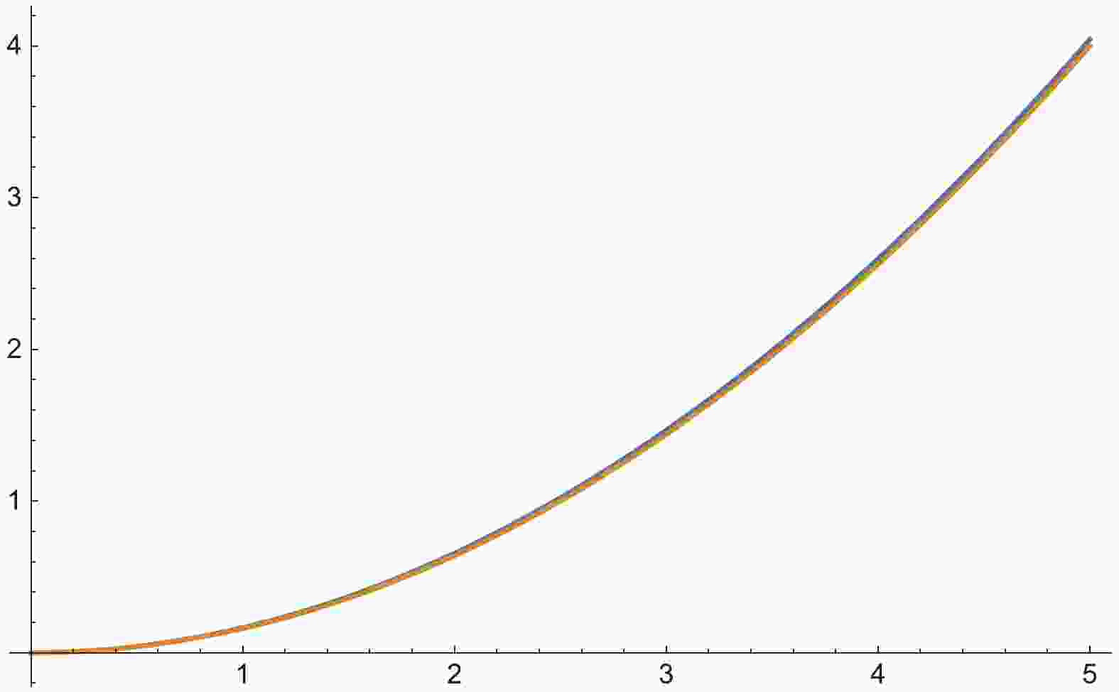
$v(z) = M z^2$ is a good approximation. The UV boundary condition$v\to z^2$ is set when solving the numerical solution. As shown in Fig. 1, the difference between the numerical and approximate solutions of$v(z)$ is very small. Further calculations find that the approximation has little effect on other numerical results. Therefore, in the following we only consider the approximation$v(z) = M z^2$ to obtain more analytical results.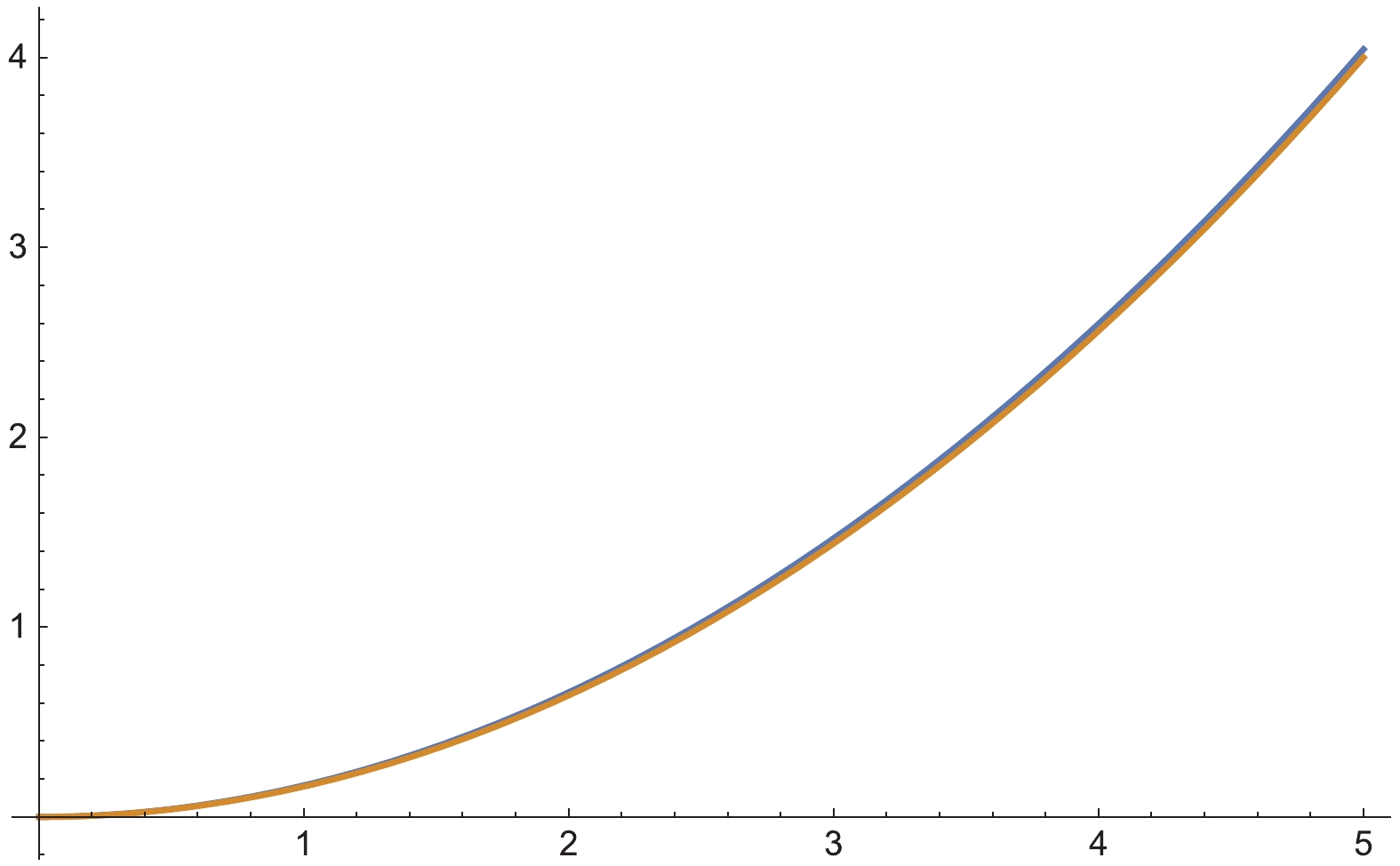
Figure 1. (color online) Difference between the numerical and approximate solutions of
$ v(z)$ . The blue and orange lines are the numerical and approximate results, respectively. -
The EOM for the scalar field
$h(x,z)$ is$\begin{aligned} -\frac{z^3}{{\rm e}^{-\phi(z)}}\partial_z \frac{{\rm e}^{-\phi}}{z^3}\partial_z h -q^2 h +\frac{1}{z^2}(m_5^2+\lambda\phi)h = 0. \end{aligned}$

(9) The solution is
$ \begin{split} h(q, z) =& C_1(q){\rm e}^{\mu z^2}z^2U\left(-\frac{q^2+\lambda\mu}{4\mu},1,-\mu z^2\right)\\ & +C_2(q){\rm e}^{\mu z^2}z^2L\left(\frac{q^2+\lambda\mu}{4\mu},-\mu z^2\right). \end{split}$

(10) Functions U and L represent Tricomi's confluent hypergeometric function and Laguerre function, respectively.
$L_{n}$ is the Laguerre polynomial. The first term represents the bulk-to-boundary propagator, and the second term gives us the KK towers of the scalar field. The normalizable solution is given as$ \begin{split} h_n(z) =& \sqrt{\frac{2}{\mu}}\mu z^2L_n(\mu z^2),\\ M_h^2(n) =& 4\mu\left(n+1+\frac{\lambda}{4}\right), \quad n = 0,1,2,... \end{split} $

(11) The orthogonality relation is
$ \int_0^\infty {\rm d}z \frac{{{\rm e}}^{-\phi(z)}}{z^3}h_n(z)h_m(z) = \delta_{nm}. $

(12) To obtain the Higgs boson of the SM,
$\lambda$ is set to$\lambda = -4+\dfrac{1}{64\mu}$ . The mass of the lowest KK excited state of the scalar field is 125 GeV. If we consider that other particles are in the TeV scale, then the Regge slope parameter$\mu$ should be greater than 1/4. This is consistent with the approximation that$\lambda$ approaches -4. -
Expanding the action in Eq. (2), the EOM of the transverse parts of the unbroken vector fields are obtained as
$ \begin{aligned} -\frac{z}{{\rm e}^{-\phi(z)}}\partial_z\left(\frac{{\rm e}^{-\phi(z)}}{z}\partial_z A_\mu^i(q,z)\right)+q^2 A_\mu^i(q,z) = 0, \end{aligned}$

(13) where
$i = 1,...,6$ and$A_z = 0$ gauge is considered, and$A_\mu^i(q,z)$ are the 4D Fourier transforms of$A_\mu^i(x,z) = \int {\rm d}^4q {\rm e}^{{\rm i}qx}A_\mu^i(q,z)$ .According to holography, the fields
$A_\mu^i(q,z)$ can be written as$ A_\mu^i(q,z) = V(q,z){{\cal{V}}}_\mu^i(q),\quad\ V(q,\epsilon) = 1. $

(14) The exact solution is
$ \begin{split} V(q,z) =& C_1(q)U\left(\frac{q^2}{4\mu},0,\mu z^2\right)\\ & +C_2(q)L\left(-\frac{q^2}{4\mu},-1,\mu z^2\right), \end{split} $

(15) where U is the Tricomi confluent hypergeometric function and L is the generalized Laguerre polynomial.
The first term represents the bulk-to-boundary propagator and the second term gives us the KK towers of the vector fields. Normalizable solutions are given as
$ \begin{split} {V_n}(z) = &\mu {z^2}\sqrt {\frac{2}{{n + 1}}} L_n^1(\mu {z^2}),\\ M_V^2(n) =& 4\mu (n + 1),\quad n = 0,1,2,... \end{split} $

(16) It can be found from the above equation that when
$\lambda$ approaches 0, the KK excited state of the scalar field and unbroken vector fields are degenerate. This means that$\lambda$ introduces splitting of the mass of the scalar field and unbroken vector fields.The
$V_n(z)$ function fulfils the following orthogonality relation:$ \int_0^\infty {\rm d}z \frac{{\rm e}^{-\phi(z)}}{z}V_n(z)V_m(z) = \delta_{nm}. $

(17) This result is similar to the results of AdS/QCD, in which the masses of vector particles are determined by
$\mu$ . -
The EOM of transverse parts of broken vector fields are
$ \left(-\frac{z}{{\rm e}^{-\phi(z)}}\partial_z \frac{{\rm e}^{-\phi(z)}}z\partial_z A_\mu^a-q^2 A_\mu^a-\frac{g_5^2 v(z)^2}{z^2}A_\mu^a\right)_\bot = 0,$

(18) where
$a = 1,\cdots,9$ and$A_z = 0$ gauge is considered.To obtain an analytical solution, we have to use the approximation
$v(z) = M z^2$ . Thus, the solution is$ \begin{split} A(q,z) =& C_1(q){\rm e}^{\textstyle\frac{(\mu-\tilde{\mu})z^2}{2}}U\left(\frac{q^2}{4\tilde{\mu}},0,\tilde{\mu}z^2\right)\\ &+ C_2(q){\rm e}^{\textstyle\frac{(\mu-\tilde{\mu})z^2}{2}}L\left(-\frac{q^2}{4\tilde{\mu}},-1,\tilde{\mu}z^2\right), \end{split}$

(19) where
$\tilde{\mu} = \sqrt{g_5^2M^2+\mu^2}$ .The first term represents the bulk-to-boundary propagator and the second term gives us the KK towers of the vector fields. Normalizable solutions are given as
$ \begin{split} A_n (z) =& \sqrt{\frac{2}{n+1}}{\rm e}^{\textstyle\frac{(\mu-\tilde{\mu})z^2}{2}}\tilde{\mu} z^2L_n^1(\tilde{\mu}z^2), \\ M_A^2(n) =& 4\tilde{\mu}(n+1) \quad n = 0,1,2,.... \end{split} $

(20) The orthogonality relation is
$ \int_0^\infty {\rm d}z \frac{ {\rm e}^{-\phi(z)}}{z}A_n(z)A_m(z) = \delta_{nm}. $

(21) We observe that the Regge trajectories of broken vector fields are similar to those of unbroken vector fields, but the slope is larger. Therefore, the broken vector states are heavier than their unbroken counterparts. It is worth noting that this conclusion is only valid when the approximation
$v = Mz^2$ is applied. This means that$\lambda$ must approach$-4$ , which is consistent with the previous result. If the numerical solution is performed, the numerical results of the vector particle spectrum are not significantly different from the analytical results, indicating that the approximation$v = Mz^2$ is suitable. -
The EOM of Goldstone bosons are
$ \partial_z \frac{{\rm e}^{-\phi(z)}}{z}\partial_z\varphi^a+\frac{{\rm e}^{-\phi(z)}g_5^2v(z)^2}{z^3}(\Pi^a-\varphi^a) = 0, $

(22) $ \frac{g_5^2v(z)^2}{z^2}\partial_z\Pi^a+q^2\partial_z\varphi^a = 0, $

(23) where
$a = 1,2,\cdots,9$ . By eliminating the$\varphi$ in the above coupled equations, we can obtainthe following equation:$ \begin{split} -\partial_z \frac{z^3}{{\rm e}^{-\phi(z)}v(z)^2}\partial_z\frac{{\rm e}^{-\phi(z)}v(z)^2}{z^3}\Pi'^a +q^2\Pi'^a+\frac{{\rm e}^{-\phi(z)}g_5^2v(z)^2}{z^2}\Pi'^a = 0, \end{split} $

(24) where
$\Pi'^a$ is the derivative of$\Pi^a$ . To obtain an analytical solution, we have to use the approximation that$v(z)\sim M z^2$ . Thus, the$\Pi'^a$ solution is$ \begin{split} \Pi'^a(q,z) =& \frac{1}{Mz}\; {\rm e}^{\frac{(\mu-\tilde{\mu})z^2}{2}}\left[C_1(q)U\left(\frac{q^2}{4\tilde{\mu}},0,\tilde{\mu}z^2\right)\right.\\ & +C_2(q)L\left.\left(-\frac{q^2}{4\tilde{\mu}},-1,\tilde{\mu}z^2\right)\right]. \end{split} $

(25) The first term represents the bulk-to-boundary propagator and the second term gives us the KK towers of the vector fields. Therefore, the mass spectra are
$ M_{\Pi}^2(n) = 4\tilde{\mu}(n+1) \quad n = 0,1,2,\cdots $

(26) It can be observed that the pseudoscalar fields and the broken vector fields are degenerate on the approximation of
$v(z) = Mz^2$ .In this model, there are nine Goldstone particles, three of which become the longitudinal parts of the W and Z bosons. The remaining six Goldstone bosons include
$UU$ ,$DD$ , and$UD$ technibaryons [30], and their electric charges are$t+1$ ,$t-1$ , and t, respectively, where t depends on the representation. Without loss of generality, let$t = -1$ , so$UU$ is the dark matter candidate TIMP. For convenience, we mark$\Pi(z)$ corresponding to the$UU$ dark matter particles$\chi(z)$ . -
In this section, SM gauge bosons and quark Yukawa coupling are introduced to the holographic model. Therefore, the masses of the W and Z bosons and the interaction between quark and dark matter particles can be obtained.
As SM gauge bosons are weakly coupled fields, they cannot be directly added to the AdS spacetime according to the holographic principle. Therefore, they are introduced into the AdS as non-dynamic fields to couple with the composite fields. Here, we introduce the redundant electroweak gauged group
$SU(2)'_L\times U(1)'_Y$ , which is broken by technicolor condensation into$U(1)'_{EM}$ . Modifying the covariant derivatives, the SM gauge field is naturally introduced into the holographic model. According to the principle of gauge invariance, the covariant derivative takes the following form:$ D_MH \to \partial_MH-{\rm i}A_MH-{\rm i}HA_M^T-{\rm i}G_MH-{\rm i}HG_M^T, $

(27) where
$ G_M = W_M^\alpha L^\alpha+Z_MY, $

(28) $ L^\alpha = \frac{S^\alpha+T^\alpha}{\sqrt{2}}, \quad Y = \frac{S^3-T^3}{\sqrt{2}}+\sqrt{2}yS^4, $

(29) with
$\alpha = 1,2,3$ . The y term in the above equation depends on the representation, and different y values correspond to different dark matter particles. In the holographic model, the specific value of y has no effect on the following results. W and Z are SM gauge fields, and are assumed to be independent of the fifth dimensional coordinate z. As the techniquark condensation breaks the electroweak symmetry, W obtains the mass$ m_W^2 = \int {\rm d}z \; {\rm e}^{-\phi}\frac{gv^2}{8z^3}. $

(30) Here, the mixed terms are omitted because we only consider the contribution of the tree level. Of course, they give one-point reducible contribution to the self-energies. If the vacuum expectation value on the approximation of
$v(z) = Mz^2$ is used, the mass of the W boson is$ m_W = \frac{gM}{2\sqrt{2\mu}}, $

(31) where g is the
$SU(2)$ gauge coupling in the SM. From the above equation we can obtain the techni-pion decay constant as$ F_\Pi = \frac{M}{\sqrt{2\mu}}. $

(32) In the SM, quarks and leptons obtain masses through Yukawa coupling. As there is no elementary scalar field in the technicolor model, it is necessary to introduce coupling terms between the composite scalar field and the quarks. To extend the SU(4) symmetry to quarks, we introduce the following vector [84]:
$ {q^j} = \left( {\begin{array}{*{20}{c}} {u_L^j}\\ {d_L^j}\\ { - {\rm i}{\sigma ^2}u_R^{j\;*}}\\ { - {\rm i}{\sigma ^2}d_R^{j\;*}} \end{array}} \right), $

(33) where j is the generation index. The quark fields are also assumed to be independent of the fifth-dimensional coordinate z. A Yukawa coupling term is then introduced into the holographic model:
$ {\cal{L}}_{Y} = -y_{u}^{ij}q^{iT}P_{u}H^{*}P_{u}q^{j}-y_{d}^{ij}q^{iT}P_{d}H^{*}P_{d}q^{j}+h.c., $

(34) $ {P_u} = {p_u}(z)\left( {\begin{array}{*{20}{c}} {{1_{2 \times 2}}}&{}\\ {}&{\dfrac{{1 + {\sigma ^3}}}{2}} \end{array}} \right), $

(35) $ {P_d} = {p_d}(z)\left( {\begin{array}{*{20}{c}} {{1_{2 \times 2}}}&{}\\ {}&{\dfrac{{1 - {\sigma ^3}}}{2}} \end{array}} \right), $

(36) where
$P_u$ and$P_d$ represent the projection operators of$SU(2)_R$ breaking into$U(1)_R$ . As the functions$p_u(z)$ and$p_d(z)$ originate from ETC interactions, their forms are related to the details of the ETC, so they are assumed to be$p_{u/d}\sim z^2$ . From Eq. (34), the Yukawa coupling term of quarks and the interaction between quarks and dark matter particles can be given as$ \begin{split} \Delta S =& -\int {\rm d}^5x \frac{{\rm e}^{-\phi}}{z^5}v(z)\sum\limits_{f = 1}^{6}p_f(z)^2\Big(y_f\bar{q}_fq_f\\ & -\frac{y_f}{2}\bar{q}_fq_f\chi^{\dagger}(z)\chi(z)\Big), \end{split}$

(37) where the dark matter particles
$\chi$ are the$UU$ components of Goldstone particles$\Pi(z)$ and the special representation of$\chi$ depends on the value of y [31]. The specific value of y has little effect on the discussion of this article, so we will not discuss it in detail. It is worth noting that the dark matter particles depend on the fifth dimensional coordinate z, whereas the quarks are independent of z. -
According to AdS/CFT duality, the two-point correlation function can be obtained as the second derivative of the action with respect to the source. Therefore, the correlation function can be written as
$ \langle {\cal{O}}(x_1){\cal{O}}(x_2)\rangle = \left. \frac{\delta^2}{\delta \phi_0[x_1]\delta \phi_0[x_2]}{\rm e}^{-S_{5}[\phi[\phi_0]]}\right|_{\phi_0 = 0}. $

(38) If the source is the vector current operator, the correlator has the following form:
$ \int {\rm d}^4x {\rm e}^{{\rm i}qx}\langle J_\mu^a(x)J_\nu^b(0)\rangle = \delta^{ab}\left(\frac{q_\mu q_\nu}{q^2}-g_{\mu\nu}\right)\Pi_V(q^2). $

(39) Considering the on-shell action (2),
$\Pi_V$ is$ \Pi_V(q^2) = \frac{1}{g_5^2}\left.\left[\frac{{\rm e}^{-\phi(z)}V(q,z)\partial_z V(q,z)}{z}\right]\right|_{z = \epsilon}. $

(40) Similar to the unbroken case, the broken-vector current correlator is given by
$ \Pi_A(q^2) = \frac{1}{g_5^2}\left.\left[\frac{{\rm e}^{-\phi(z)}A(q,z)\partial_z A(q,z)}{z}\right]\right|_{z = \epsilon}. $

(41) From holography, the KK part of V and A has a negligible effect on the correlator, and only the bulk-to-boundary propagator is significant. Substituting the propagator from Eq. (15), the unbroken vector correlator is given as
$ \Pi_V(q^2) = \frac{q^2}{2g_5^2}\left(2\gamma_E+{\rm{ln}}\; \mu z^2+\psi\left(1+\frac{q^2}{4\mu}\right)\right), $

(42) with
$\gamma_E$ is the Euler constant and$\psi$ is the digamma function. Here we use the boundary condition of$V(q,\epsilon) = 1$ .Similarly, broken vector correlator can be obtained from Eq. (19)
$ \Pi_A(q^2) = \frac{\mu-\tilde{\mu}}{g_5^2}+\frac{q^2}{2g_5^2}\left(2\gamma_E+{\rm{ln}}\; \tilde{\mu} z^2+\psi\left(1+\frac{q^2}{4\tilde{\mu}}\right)\right). $

(43) Again, we use the boundary condition of
$A(q,\epsilon) = 0$ . It can be observed that when$\mu = \tilde{\mu}$ , the correlators of the unbroken and broken vectors are consistent. In this case, the technicolor condensate$M = 0$ and the$SU(4)$ symmetry is unbroken.The S and T of the Peskin–Takeuchi parameters are important for the exploration of new physics. Due to the presence of custodial symmetry, T disappears in this model, and thus, only S parameters are considered. S parameters can be obtained using unbroken and broken vector correlators [85]
$ S = \left. -4\pi \frac{\rm d}{{\rm d}q^2}(\Pi_V-\Pi_A)\right|_{q^2\to 0} = \frac{2\pi}{g_5^2}{\rm{ln}}\; \frac{\tilde{\mu}}{\mu}. $

(44) According to the definition of
$\tilde{\mu}$ ,$\tilde{\mu}$ is greater than$\mu$ , and thus S is positive. We can also obtain the decay constant of a techni-pion:$ F_\Pi^2 = \Pi_V(0)-\Pi_A(0) = \frac{\tilde{\mu}-\mu}{g_5^2}. $

(45) We can observe that the results of (32) and (45) seem to be inconsistent. However, if we consider the approximation of
$\mu \gg g_5M$ , the results of (45) will become (32). Based on the approximation, the S parameter will become$ S\simeq \frac{2\pi F_\Pi^2}{\mu}, $

(46) which is consistent with the strong dynamics
$S\approx 4\pi F_\Pi^2(M_V^{-2}+M_A^{-2})$ [86].In the holographic model, if the Yukawa term is not included, there are four parameters:
$N_{TC}$ , M,$\mu$ and$\lambda$ . As the color$N_{TC}$ of technicolor has little effect on the result, it is fixed to$2$ . Fitting the masses of the Higgs boson and W boson, the model has only one free parameter$\mu$ , i.e., the Regge slope of the particles. As can be seen from Eq. (44) and Fig. 2, the S parameter monotonically decreases as$\mu$ increases. From the PDG [87], the S parameter is required to be within the range:$-0.08\leqslant S \leqslant 0.12$ or$-0.05\leqslant S \leqslant 0.09$ ($U = 0$ is fixed). Therefore, it can be seen from Eq. (44) that$\mu$ must satisfy$\mu\gtrsim 0.83$ or$\mu\gtrsim 1.6$ . The$F_\Pi$ term of Eq. (45) monotonically increases as$\mu$ becomes larger. If the difference between (45) and (32) is less than 10%, then$\mu$ must satisfy$\mu \gtrsim 6.15$ .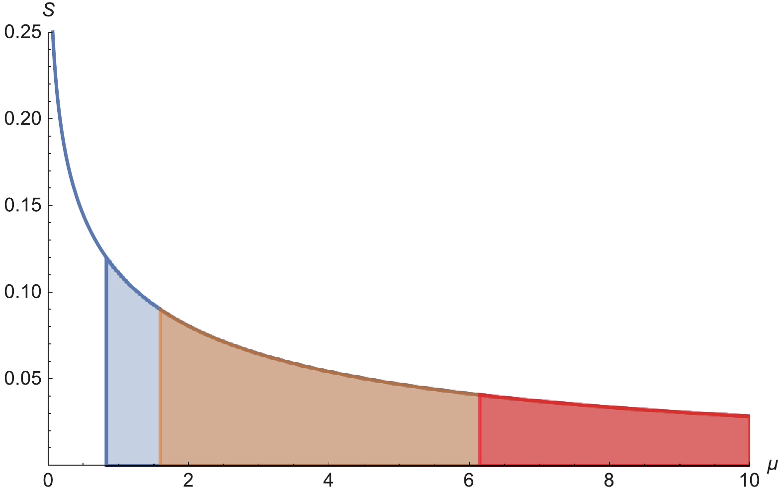
Figure 2. (color online) Range of values of S and
$ \mu$ when different conditions are satisfied. The blue region indicates that$ -0.08\leqslant S \leqslant 0.12$ ; the orange region indicates that$ -0.05\leqslant S \leqslant 0.09$ ; the red region indicates that Eqs. (32) and (45) are consistent. -
In this section, we will consider dark matter particles in the holographic model. In the model, the dark matter particles are pseudo-Goldstone particles produced by spontaneous symmetry breaking. The dark matter particles have a technibaryon number, and thus, during the cosmic electroweak phase transition, enough dark matter is produced by the sphaleron process [31]. Through the sphaleron process, baryon energy density can be linked with dark matter density. When the mass of the dark matter is about
$2.2$ TeV, the relic density can be obtained [88].In the holographic technicolor model, TIMPs interact with quarks mainly through Yukawa couplings and by exchanging Z bosons, which can be obtained from (27) and (34). Numerical calculations show that the effect of exchanging Z bosons on the final result is negligible; therefore, we mainly consider the impact of the Yukawa coupling terms on direct detection. By calculating the cross-sections of dark matter and nuclei, the parameter space of the model can be constrained. Due to the dark matter relic density, we mainly focus on the TeV scale region. It can be seen from (37) that the Yukawa coupling
$y_f$ is adjusted to fit the quark mass, and the effective coupling constants of the interaction between the dark matter particles and quarks can be obtained. Thus, the quark mass can be given as$ m_f = y_f\int_{0}^{\infty}{\rm d}z\frac{{\rm e}^{-\phi}}{z^5}v(z)p_f(z)^2, $

(47) where f is flavor of quarks. It is worth noting that the above equation contains the unknown function
$p_f$ , which is derived from the ETC interaction. We assume that its behavior is$p_f = z^2$ , i.e., that it has a similar form to the vacuum expectation value$v(z)$ . As the coefficient of the function can be absorbed into$y_f$ , it is set to$1$ . The effective coupling constant$F_f$ is$ F_f = -\frac{y_f}{2}\int_{0}^{\infty}{\rm d}z\frac{{\rm e}^{-\phi}}{z^5}v(z)p_f(z)^2\chi^{\dagger}(z)\chi(z), $

(48) where
$\chi (z)$ is given by Eq. (25). Equation (25) only gives the derivative of$\chi$ , and an additional boundary condition needs to be added. By selecting the boundary condition$\Pi''(z\to\infty) = \Pi'(\epsilon) = \Pi(\epsilon) = 0$ , the dark matter$\chi$ can be solved and the effective coupling constants can be given.The dark matter nucleus cross-section can be obtained by the following [89]:
$ \sigma_{SI} = \frac{m_N^2}{4\pi(M_{DM}+m_N)^2}\left(\frac{F_N}{\sqrt{2}}\right)^2, $

(49) where
$M_{DM}$ and$m_N$ are the dark matter mass and nucleus mass, respectively, and$F_N$ is the induced coupling constant of dark matter–nucleus interactions.$F_N$ and$F_f$ are related by$ F_N = \sum\limits_{f = u,d,s}F_ff_f^N\frac{m_N}{m_f}+\sum\limits_{f = c,b,t}F_ff_Q^N\frac{m_N}{m_f}, $

(50) with the nucleon form factors
$f_u^p = 0.020\pm0.004$ ,$f_d^p = 0.026\pm0.005$ ,$f_s^p = 0.118\pm0.062$ ,$f_u^n = 0.014\pm0.003$ ,$f_d^n = 0.036\pm0.008$ ,$f_s^n = 0.118\pm0.062$ , and$f_Q^N = \dfrac{2}{27}(1- f_u^N-f_d^N-f_s^N)$ for heavy quarks [90, 91].The dark matter–nucleon scattering cross-section can be obtained using the effective coupling constant, as shown in Fig. 3. Fig. 3 shows that the orange part has been excluded by the XENON1T experiment. The cross-section decreases as the mass of the dark matter increases, and intersects the XENON1T experimental data at approximately
$2$ TeV. Therefore, the case where the mass is less than$2$ TeV has been ruled out by the experiment, that is,$\mu\lesssim 0.14$ . Considering the possible range of direct detection for future experiments, we focus on the case where the cross-section is$10^{-45}\sim 10^{-48}\;{\rm{cm}}^2$ . In other words, we pay more attention to the situation in which the dark matter mass is at$2\sim4$ TeV, corresponding to$1.79\gtrsim\mu\gtrsim 0.14$ . For the case where the mass is greater than 4 TeV, as the dark matter particles are difficult to detect, the constraint on the holographic model is small.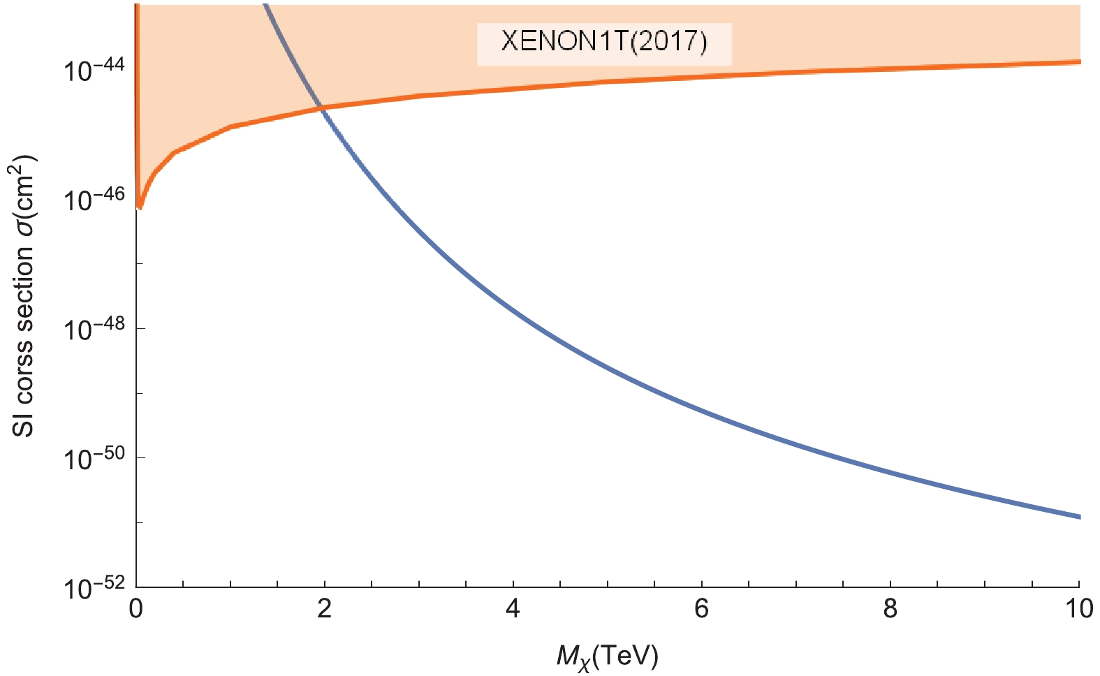
Figure 3. (color online) Spin-independent (SI) dark matter–nucleon cross-sections: The blue line is the result of the holographic dark matter particles
$ \chi$ ; the orange line is the experimental data of XENON1T [92].When the dark matter mass is considered to be much larger than the electroweak phase transition temperature, the dark matter mass estimated by the electroweak sphaleron process is approximately 2 TeV [88], which is consistent with the lower limit estimated by direct detection in the holographic model. This means that the mass of dark matter in the model that satisfies direct detection can explain the relic density
$\Omega_{DM}/\Omega_{B}\sim5$ . For the case where the electroweak phase transition temperature is much larger than the dark matter mass, the dark matter mass estimated by the sphaleron phase transition is approximately 5 TeV [88]. The upper mass limit calculated in the holographic model means that the phase transition temperature is comparable to the dark matter mass. Heavier dark matter, that is, a larger parameter$\mu$ , is associated with higher electroweak phase transition temperature.Further, considering the constraints of the S parameter, the range of the parameter
$\mu$ is$1.79\gtrsim\mu \gtrsim 0.83$ or$1.79\gtrsim\mu\gtrsim 1.6$ , that is, the dark matter mass is$4$ TeV$\gtrsim M_{DM} \gtrsim 3.22$ TeV or$4$ TeV$\gtrsim M_{DM} \gtrsim 3.88$ TeV, respectively. The constraint of the S parameter requires the model to have heavier dark matter, and the SI section is$10^{-47}\sim10^{-48}$ cm2, which implies a higher phase transition temperature in the holographic technicolor model. The consistency of Eq. (32) and Eq. (45) requires that$\mu$ > 6.15, which makes the cross-section of the dark matter and nucleus too small, and therefore, this is not in the scope of this study.In summary, considering the constraints of the relic density, SI cross-section, and S parameter, the dark matter mass is approximately
$4$ TeV$\gtrsim M_{DM} \gtrsim 3.22$ TeV or$4$ TeV$\gtrsim M_{DM} \gtrsim 3.88$ TeV. In this case, the SI cross-section is$10^{-47}\sim10^{-48}$ cm2, and the relic density requires that the phase transition temperature be comparable to the dark matter mass. -
In this study, we studied dynamical electroweak symmetry breaking and dark matter using gauge/gravity duality. We successfully constructed a holographic technicolor model, that is dual to the MWT model, with
$N_{TC} = 2$ , in which the W and Z bosons obtained masses by technicolor condensation. In addition, we calculated the Peskin–Takeuchi S parameters and obtained many particles at the TeV energy scale, including dark matter candidate TIMPs.In this holographic model, similar to QCD, the gauge boson obtains mass by technicolor condensation, and the
$125$ GeV boson, similar to$\sigma$ particle in QCD, is a composite Higgs boson. If the mass of the Higgs and W bosons is fitted, the holographic model has only one free parameter$\mu$ left.$\mu$ describes the Regge slope of technihadrons and determines their mass. The S parameter is used to constrain the parameter space of the new physics and its experimental range is$-0.08\leqslant S \leqslant 0.12$ or$-0.05\leqslant S \leqslant 0.09$ ($U = 0$ is fixed). As in the holographic model the S parameter decreases as$\mu$ increases,$\mu$ needs to satisfy$\mu\gtrsim 0.83$ or$\mu\gtrsim 1.6$ .Dark matter candidate particles TIMPs are among the many technihadrons of the holographic model. By adding the Yukawa coupling term, the holographic model can obtain the effective coupling constant of the dark matter and quarks, and further obtain the spin-independent dark matter–nucleon cross-section
$\sigma_{SI}$ . We found that the cross-section in the model decreases as the mass of the dark matter increases, and the theoretical line intersects the XENON1T experimental line at a dark matter mass of approximately$2$ TeV. If we are concerned with the range of$10^{-45}\sim 10^{-48}$ cm$^2$ that may be detected in future experiments, the dark matter mass is limited to$2\sim4$ TeV. If both the S parameter and dark matter cross-section constraints are considered, the mass of dark matter is$3.2\sim 4$ TeV or$3.8\sim 4$ TeV.
Holographic technicolor model and dark matter
- Received Date: 2019-12-31
- Accepted Date: 2020-05-01
- Available Online: 2020-09-01
Abstract: We investigate the strongly coupled minimal walking technicolor model (MWT) in the framework of a bottom-up holographic model, where the global


 DownLoad: