Study on the possible molecular state composed of ${{D}^ * _s} {\bar{{D}}_{{s1}}}$ within the Bethe-Salpeter framework

In 2019, the Belle Collaboration observed a vector charmonium-like state $Y(4626)$ in the portal of $e^+e^- \to D^+_sD_{s1}(2536)^-+c.c.,$ and its mass and width are $4625.9^{+6.2}_{-6.0}({\rm{stat.}} )\pm0.4({\rm{syst.}} )$ MeV and $49.8^{+13.9}_{-11.5}({\rm{stat.}} )\pm 4.0({\rm{syst.}} )$ MeV, respectively [1]. In 2008, the Belle Collaboration reported a near-threshold enhancement in the $e^+e^-\to \Lambda_c^+\Lambda_c^-$ cross section, and the peak corresponds to a hadronic resonance, which is named as $Y(4630)$ [2]. Recently, a simultaneous fit was performed to the data analysis of $e^+e^-\to \Lambda_c^+\Lambda_c^- ,$ and a peak with mass and width being $4636.1^{+9.8}_{-7.2}({\rm{stat.}} )\pm8.0({\rm{syst.}} )$ MeV and $34.5^{+21.0}_{-16.2}({\rm{stat.}} )\pm$$5.6({\rm{syst.}} )$ MeV, respectively was observed [3]. Due to their very close masses and widths, it is natural to consider that $Y(4626)$ and $Y(4630)$ are the same resonances. In Ref. [4], the authors explained $Y(4626)$ and $Y(4660)$^① [5] to be mixtures of two excited charmonia. This may also be a non-resonant threshold enhancement due to the opening of the $\Lambda_c^+\Lambda_c^-$ channel as discussed in [6, 7], whereas the authors [8] suggested $Y(4626)$ as a molecular state $D^*_s\bar D_{s1}(2536)$. In Refs. [9, 10] $Y(4626)$ was regarded as a tetraquark $cs\bar c \bar s$.

Since 2003, many exotic resonances of X, Y, and Z bosons [11-20] have been experimentally observed, such as $X(3872)$, $X(3940)$, $Y(3940)$, $Z(4430)$, $Y(4260)$, $Z_c$(4020), $Z_c$(3900), $Z_b(10610) ,$ and $Z_b(10650)$ (of course, this is not a complete list). These states have attracted the attention of theorists because their structures are obviously beyond the simple $q\bar q$ settings for mesons. If we can firmly determine their compositions, it would definitely enrich our knowledge on hadron structures and moreover, shed light on the non-perturbative quantum chromodynamic (QCD) effects at lower energy ranges. Studies with different explanations of the inner structures [21] have been attempted, such as in terms of the molecular state, tetraquark, or dynamical effects [22]. Although all the ansatz have a certain reasonability, a unique picture or criterion for firmly determining the inner structures is still lacking. Nowadays, the majority of phenomenological researchers conjecture what the concerned exotic states are composed of, simply based on the available experimental data. Then, by comparing the results with new data, one can verify the degree of validity of the proposal. If the results obviously contradict the new measurements that have better accuracy, the ansatz should be abandoned. Following this principle, we explore $Y(4626)$ by assuming it to be a molecular state of $D^*_s\bar D_{s1}(2536)$, and then, by using a more reliable theoretical framework, we verify the scenario and see if the proposal based on our intuition is valid.

Thus, in this work, we suppose $Y(4626)$ as a $D^*_s\bar D_{s1}(2536)$ molecular state, and we employ the Bethe-Salpeter (B-S) equation, which is a relativistic equation established on the basis of quantum field theory, to study the two-body bound state [23]. Initially, the B-S equation was used to study the bound state of two fermions [24-26]. Subsequently, the method was generalized to the system of one-fermion-one-boson [27]. In Refs. [28, 29], the authors employed the Bethe-Salpeter equation to study some possible molecular states, such as the $K\bar K$ and $B\bar K$ systems. Using the same approach, the bound states of $B\pi$, $D^{(*)}D^{(*)}$, and $B^{(*)}B^{(*)}$ are studied [30, 31]. Recently, the approach was applied to explore doubly charmed baryons [32, 33] and pentaquarks [34, 35]. In this work, we try to calculate the spectrum of $Y(4626)$ composed of a vector meson and an axial vector meson.

If two constituents can form a bound state, the interaction between them should be large enough to hold them into a bound state. The chiral perturbation theory tells us that two hadrons interact via exchanging a certain mediate meson(s) and the forms of the effective vertices are determined by relevant symmetries; however, the coupling constants generally are obtained by fitting data. For the molecular states, since two constituents are color-singlet hadrons, the exchanged particles are some light mesons with definite quantum numbers. It is noted that even though there are many possible light mesons contributing to the effective interaction between the two constituents, generally one or several of them would provide the dominant contribution. Further, the scenario with other meson exchanges should also be considered, because even though the extra contributions are small compared to the dominant one(s), they sometimes are not negligible, i.e., they would make a secondary contribution to the effective interaction. Then, the effective kernel for the B-S equation can be set. For the $D^*_s\bar D_{s1}(2536)$ system, the contribution of $\eta$ [36-38] dominates, whereas in Ref. [36] the authors suggested $\sigma$ exchange makes the secondary contribution. In our case that considers the concerned quark contents of $D^*_s$ and $\bar D_{s1}(2536)$, the contribution of {$\eta'$, $f_0(980)$ and $\phi$} should stand as the secondary type. The effective interactions induced by exchanging {$\eta$, $\eta'$, $f_0(980)$ and $\phi$} are deduced with the heavy quark symmetry [36-41], and we have presented these formulas in Appendix A. Based on the effective interactions, we can derive the kernel and establish the corresponding B-S equation.

With all necessary parameters being chosen beforehand and provided as inputs, the B-S equation is solved numerically. In some cases, the equation does not possess a solution if one or several parameters are set within a reasonable range; in such cases, a conclusion is drawn that the proposed bound state does not exist in nature. On the contrary, a solution of the B-S equation with reasonable parameters implies that the corresponding bound state is formed. In such a case, the B-S wave function is obtained simultaneously, which can be used to calculate the rates of strong decays; this would in turn enable experimentalists to design new experiments for further measurements.

This paper is organized as follows: following the introduction section, a derivation of the B-S equation related to a possible bound state composed of $D^*_s$ and $\bar D_{s1}(2536)$, which are a vector meson and an axial vector meson, respectively, is provided. In Section 3, the formulas for its strong decays are presented. Then, in Section 4, we present the numerical solution of the B-S equation. Since $Y(4626)$ is supposed to be a molecular bound state, the input parameters must be within a reasonable range. However, our results show that this mandatory condition cannot be satisfied, and therefore, we think that such a molecular state of $D^*_s\bar D_{s1}(2536)$ may not exist. Further, as we have deliberately set the parameters to a region that is not favored by any of the previous phenomenological works, we can obtain the required spectrum and corresponding wavefunctions. Using the wavefunction, we evaluate the strong decay rate of $Y(4626)$ and present our results in the form of figures and tables. Finally, a brief summary of our work is provided in Section 4.

Since the newly observed resonance $Y(4626)$ contains hidden charms and its mass is close to the sum of the masses of $D^*_s$ and $\bar D_{s1}$, where $D^*_s-\bar D_{s1}$ corresponds to $D^{*+}_s- D_{s1}^-$ or $D^{*-}_s- D_{s1}^+$, a conjecture about its molecular structures composed of $D^*_s$ and $\bar D_{s1}$ is favored. For a state with spin-parity being $1^-$, its spatial wave function is in the S wave. Therefore, there are two possible states, namely, $Y_1 = \dfrac{1}{\sqrt{2}}( D^{*+}_s D_{s1}^-+ D^{*-}_s D_{s1}^+)$ and $Y_2 = \dfrac{1}{\sqrt{2}}( D^{*+}_s D_{s1}^- D^{*-}_s D_{s1}^+)$. We will focus on such an ansatz and try to determine numerical results by solving the relevant B-S equation.

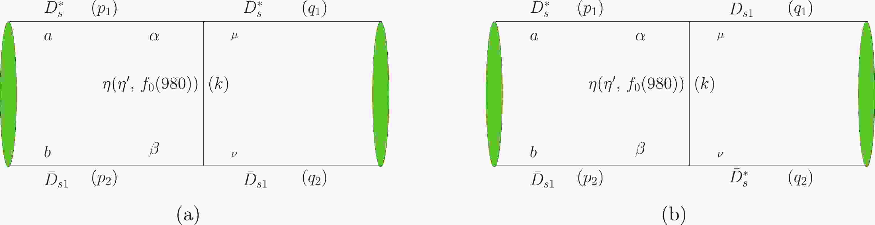
Based on the effective theory, $D^*_s$ and $\bar D_{s1}$ interact mainly via exchanging $\eta$. The Feynman diagram at the leading order is depicted in Fig. 1. To take into account the secondary contribution induced by exchanging other mediate mesons, in Ref. [36], the authors consider a contribution of exchanging $\sigma$ to the effective interaction. Since there are neither u nor d constituents in $D^*_s$ and $\bar D_{s1}$, their coupling to $\sigma$ would be very weak; thus, the secondary contribution to the interaction may arise from exchanging $f_0(980)$ instead. The relevant Feynman diagrams are shown in Fig. 1. In this work, the contributions induced by exchanging $\eta'$ (Fig. 1) and $\phi(1020)$ (Fig. 2) are also taken into account. The relations between relative and total momenta of the bound state are defined as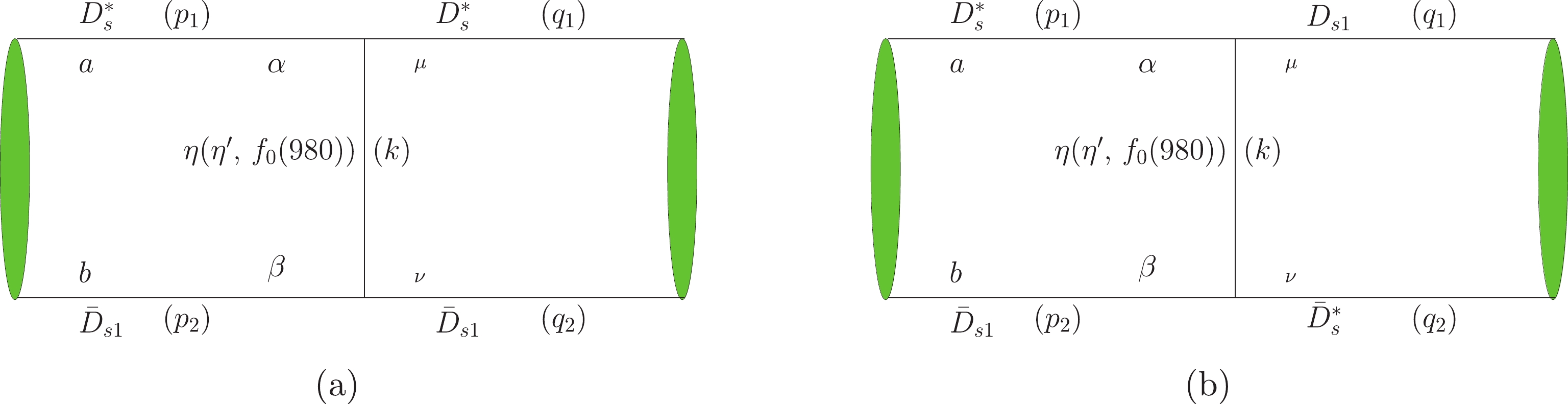

Figure 1.  (color online) The bound states of $D^*_s \bar D_{s1}$ formed by exchanging $\eta\,(\eta')\,f_0(980)$.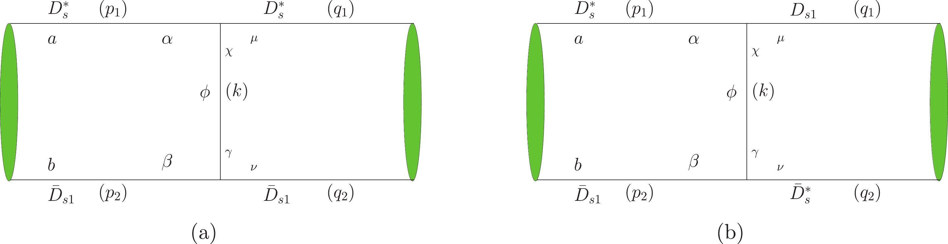

Figure 2.  (color online) The bound states of $D^*_s \bar D_{s1}$ formed by exchanging $\phi(1020)$.

where $p_1$ and $p_2$ ($q_1$ and $q_2$) are the momenta of the constituents; p and q are the relative momenta between the two constituents of the bound state at the both sides of the diagram; P is the total momentum of the resonance; $\eta_i = m_i/(m_1+m_2)$ and $m_i\, (i = 1,2)$ is the mass of the i-th constituent meson, and k is the momentum of the exchanged mediator.

A detailed analysis on the Lorentz structure [26, 28, 29] is used to determine the form of the B-S wave function of the bound state comprising a vector meson and an axial vector meson ($D^*_s$ and $\bar D_{s1}$) in $S-$wave as the following:

where $a, b, c,$and d are Lorentz indices. The wave function in the momentum space can be obtained by carrying out a Fourier transformation:

Using the so-called ladder approximation, one can obtain the B-S equation deduced in earlier references [23-25]:

where $\Delta_{1a\alpha}$ and $\Delta_{2b\beta}$ are the propagators of $D^*_s$ and $\bar D_{s1}$ respectively, and $K^{\alpha\beta\mu\nu}(P,p,q)$ is the kernel determined by the effective interaction between two constituents, which can be calculated from the Feynman diagrams in Figs. 1 and 2. In order to solve the B-S equation, we decompose the relative momentum p into the longitudinal component $p_l$ ($= p\cdot v$) and the transverse one $p^\mu_t$ ($= p^\mu-p_lv^\mu$) = (0, ${{p}}_T$) with respect to the momentum of the bound state P ($P = Mv$).

where M is the mass of the bound state $Y(4626)$, $\omega_i = \sqrt{{ {{p}}_T}^2 + m_i^2}$.

From the Feynman diagrams shown in Figs. 1 and 2, the kernel $K^{\alpha\beta\mu\nu}(P,p,q)$ can be written as

where $m_{\eta(\eta',\phi,f_0)}$ is the mass of the exchanged meson $\eta(\eta',\phi(1020),f_0(980))$, ${\cal{C}}_1$ = 1 for $Y_1$ and -1 for $Y_2$, ${\cal{C}}_2$ = 1, $g_{_{D_{s1}D^*_{s}\eta}}$, $g_{_{\bar D_{s1}\bar D^*_{s}\eta}}$, $g_{_{D^*_{s}D^*_{s}\eta}}$, $g_{_{\bar D_{s1}\bar D_{s1}\eta}}$,$g_{_{D_{s1}D^*_{s}\eta'}}$, $g_{_{\bar D_{s1}\bar D^*_{s}\eta'}}$, $g_{_{D^*_{s}D^*_{s}\eta'}}$, $g_{_{\bar D_{s1}\bar D_{s1}\eta'}}$, $g_{_{D_{s1}D^*_{s}\phi}}$, $g_{_{\bar D_{s1}\bar D^*_{s}\phi}}$, $g_{_{D^*_{s}D^*_{s}\phi}}$, $g_{_{\bar D_{s1}\bar D_{s1}\phi}}$, $g'_{_{D^*_{s}D^*_{s}\phi}}$, $g'_{_{\bar D_{s1}\bar D_{s1}\phi}}$, $g_{_{D^*_{s}D^*_{s}f_0}}$ and $g_{_{\bar D_{s1}\bar D_{s1}f_0}}$ are the concerned coupling constants and $\Delta(k,m) = {\rm i}/(k^2-m^2)$. Due to the small coupling constants at the vertices, the contribution of $f_0(980)$ in Fig. 1(b) is suppressed compared with that in Fig. 1(a), so that we ignore the contribution of $f_0(980)$ in Eq. (7). All the effective interactions are summarized and listed in the Appendix.

Since the two constituents of the molecular state are not on-shell, at each interaction vertex a form factor should be introduced to compensate the off-shell effect. The form factor is employed in many Refs. [42-45], even though it has different forms. Here we set it as:

where ${{k}}$ is the three-momentum of the exchanged meson and $\Lambda$ is a cutoff parameter. Indeed, the form factor is introduced phenomenologically and there lacks any reliable knowledge on the value of the cutoff parameter $\Lambda$. $\Lambda$ is often parameterized to be $\lambda\Lambda_{\rm QCD}+m_s$ with $\Lambda_{\rm QCD} = 220$ MeV, which is adopted in some Refs. [42-45]. As suggested, the order of magnitude of the dimensionless parameter $\lambda$ should be close to 1. In our subsequent numerical computations, we set it to be within a wider range of $0\sim 4$.

The wave function can be written as

where $\epsilon$ is the polarization vector of the bound state and $f({ p})$ is the radial wave function. The three-dimension spatial wave function is obtained after integrating over $p_l$

Substituting Eqs. (7) and (9) into Eq. (4) and multiplying $\varepsilon_{abfg}\chi^{*g}_P(x_1,x_2)P^f$ on both sides, one can sum over the polarizations of both sides. Employing the so-called covariant instantaneous approximation [46] $q_l = p_l ,$ i.e., using $p_l$ to replace $q_l$ in $K(P,p,q)$, the kernel $K(P,p,q)$ does not depend on $q_1$ any longer. Then, we follow a typical procedure: integrating over $q_l$ on the right side of Eq. (4), multiplying $\int\dfrac{{\rm d}p_l}{(2\pi)}$ on both sides of Eq. (4), and integrating over $p_l$ on the left side, to reduce the expression into a compact form. Finally, we obtain

with

While we integrate over $p_l$ on the right side of Eq. (11), there exist four poles that are located at $-\eta_1M-\omega_1+{\rm i}\epsilon$, $-\eta_1M+\omega_1-{\rm i}\epsilon$, $\eta_2M+\omega_2-{\rm i}\epsilon$ and $\eta_2M-\omega_2+{\rm i}\epsilon$. By choosing an appropriate contour, we only need to evaluate the residuals at $p_l = -\eta_1M-\omega_1+{\rm i}\epsilon$ and $p_l = \eta_2M-\omega_2+{\rm i}\epsilon$.

Here, since ${\rm d}^3{{q}}_T = {{q}}_T^2{\rm{sin}}(\theta){\rm d}|{{q}}_T|{\rm d}\theta {\rm d}\phi$ and ${{p}}_T\cdot {{q}}_T = |{{p}}_T||{{q}}_T|$${\rm{cos}}(\theta)$, one can integrate the azimuthal part, and then, Eq. (11) is reduced into a one-dimensional integral equation:

with

Analogous to the cases in Refs. [28, 29], the normalization condition for the B-S wave function of a bound state should be

where $P_0$ is the energy of the bound state, which is equal to its mass M in the center of mass frame. $I(P,p,q)$ is a product of reciprocals of two free propagators with a proper weight.

In our earlier work [31], we found that the term $K^{ab\alpha\beta}(P,p,q)$ in brackets is negligible; hence, we ignore it as done in Ref. [47].

To reduce the singularity of the problem, we ignore the second item in the numerators of the propagators (Eq. (5) and (6)) and $(\Delta^{a\alpha}_1)^{-1} = -{\rm i}g^{a\alpha}(p_1^2-m_1^2)$, $(\Delta^{b\beta}_1)^{-1} =$$-{\rm i}g^{b\beta}(p_2^2-m_2^2)$. Then, the normalization condition is

After performing some manipulations, we obtain the normalization of the radial wave function as the following:

Next, we investigate the strong decays of $Y(4626)$ using the effective interactions, which only includes contributions induced by exchanging $\eta$ and $\eta'$. Subsequently, we will discuss this issue further.

The relevant Feynman diagram is depicted in Fig. 3(a) where $\bar D_{s0}$ represents $\bar D_{s0}(2317)$. The amplitude is,

Figure 3.  (color online) The decays of $Y(4626)$ by exchanging $\eta(\eta')$.

where $k = p-(\eta_2 q_1-\eta_1 q_2)$, and $\epsilon_1$ is the polarization vector of $D^*_s$. We still consider the approximation $k_0 = 0$ to perform the calculation.

The amplitude can be parameterized as [48]

The factors $g_0$ and $g_2$ are extracted from the expressions of ${\cal{A}}_a$.

Then, the partial width is expressed as

The corresponding Feynman diagram is depicted in Fig. 3(b) where $\bar D'_{s1}$ denotes $D_s(2460)$ in the rest of the manuscript. Then, the amplitude can be defined as

The amplitude can also be parameterized as

where $\epsilon_2$ is the polarizations of $\bar D_s(2460)$. The factors $g'_0$ and $g'_2$ can be extracted from the expressions of ${\cal{A}}_b$.

The Feynman diagram for the process of $Y(4626)\to$$D_s(2460)(1^+)+\bar D^*_s(1^-)$ is depicted in Fig. 3(c). Then, the amplitude is given as

where $\epsilon_1$ and $\epsilon_2$ are the polarization vectors of $D_s(2460)$ and $\bar D^*_s$, respectively. The total amplitude can be parameterized as [48]

The factors $g_{10}$, $g_{11}$ and $g_{12}$ are extracted from the expressions of ${\cal{A}}_c$.

The Feynman diagram for $Y(4626)\to D^*_s(1^-)+$$\bar D_s(2460)(1^+)$ is depicted in Fig. 3(d). The amplitude is

where $\epsilon_1$ and $\epsilon_2$ are the polarization vectors of $D^*_s$ and $\bar D_s(2460)$, respectively.

The total amplitude for the strong decay of $Y(4626)\to D^*_s(1^-)+\bar D_s(2460)(1^+)$ can also be expressed as

The factors $g'_{10}$, $g'_{11}$ and $g'_{12}$ are extracted from the expressions of ${\cal{A}}_d$.

The Feynman diagram is depicted in Fig. 3(e) where $\bar D_{s2}$ represents $\bar D_s(2572)$. Then, the amplitude is defined as follows:

where $\epsilon_2$ is the polarization tensor of $\bar D_s(2572)(2^+)$.

The total amplitude is written as

The factors $g_{20}$ can be extracted from the expressions of ${\cal{A}}_e$.

The Feynman diagram is depicted in Fig. 3(f) where $\bar D_{s1}$ represents $\bar D_s(2536)$. The amplitude is then given as

where $\epsilon_2$ is the polarization vector of $D_s(2536)$.

The amplitude is still written as

The factors $g''_0$ and $g''_2$ are extracted from the expressions of ${\cal{A}}_f$.

Before we numerically solve the B-S equation, all necessary parameters should be priori determined as accurately as possible. The masses $m_{D^*_s}$, $m_{D_{s0}}$, $m_{D_{s1}}$, $m_{D'_{s1}}$, $m_{D_{s2}}$, $m_\eta$, $m_{\eta'}$, $m_{f_0(980)}$ and $m_\phi$ are obtained from the databook [49]. The coupling constants in the effective interactions $g_{_{D_{s1}D^*_{s}\eta}}$, $g_{_{\bar D_{s1}\bar D^*_{s}\eta}}$, $g_{_{D^*_{s}D^*_{s}\eta}}$, $g_{_{\bar D_{s1}\bar D_{s1}\eta}}$,$g_{_{D_{s1}D^*_{s}\eta'}}$, $g_{_{\bar D_{s1}\bar D^*_{s}\eta'}}$, $g_{_{D^*_{s}D^*_{s}\eta'}}$, $g_{_{\bar D_{s1}\bar D_{s1}\eta'}}$, $g_{_{D_{s1}D^*_{s}\phi}}$, $g_{_{\bar D_{s1}\bar D^*_{s}\phi}}$, $g_{_{D^*_{s}D^*_{s}\phi}}$, $g_{_{\bar D_{s1}\bar D_{s1}\phi}}$, $g'_{_{D^*_{s}D^*_{s}\phi}}$, $g'_{_{\bar D_{s1}\bar D_{s1}\phi}}$, $g_{_{D^*_{s}D^*_{s}f_0}}$ and $g_{_{\bar D_{s1}\bar D_{s1}f_0}}$ are taken from the relevant literature and their values and related references are summarized in the Appendix.

With these input parameters, the B-S equation Eq. (12) can be solved numerically. Since it is an integral equation, an efficient way for solving it is by discretizing it and then in turn, solving the integral equation to an algebraic equation group. Effectively, we let the variables ${{|p_T|}}$ and ${{|q_T|}}$ be discretized into n values $Q_1$, $Q_2$,...$Q_n$ (when $n>100,$ the solution is stable enough, and we set n = 129 in our calculation) and the equal gap between two adjacent values as $\dfrac{Q_n-Q_1}{n-1}$. Here, we set $Q_1$ = 0.001 GeV and $Q_n$ = 2 GeV. The n values of $f(|{{p}_T}|)$ constitute a column matrix on the left side of the equation and the n elements $f({{|q_T|}})$ constitute another column matrix on the right side of the equation as shown below. In this case, the functions in the curl bracket of Eq. (12) multiplied by ${\dfrac{|{{q}}_T|^2}{12M^2(2\pi)^2}}$ would be an effective operator acting on $f({{|q_T|}})$. It is specially noted that because of discretizing the equation, even ${\dfrac{|{{q}}_T|^2} {12M^2(2\pi)^2}}$ turns from a continuous integration variable into n discrete values that are involved in the $n\times n$ coefficient matrix. Substituting the n pre-set $Q_i$ values into those functions, the operator transforms into an $n\times n$ matrix that associates the two column matrices. It is noted that $Q_1$, $Q_2$,...$Q_n$ should assume sequential values.

As is well known, if a homogeneous equation possesses non-trivial solutions, the necessary and sufficient condition is that det$|A(\Delta E,\lambda)-I| = 0$ (I is the unit matrix), where $A(\Delta E,\lambda)$ is simply the aforementioned coefficient matrix. Thus, solving the integral equation simplifies into an eigenvalue searching problem, which is a familiar concept in quantum mechanics; in particular, the eigenvalue is required to be a unit in this problem. Here, $A(\Delta E,\lambda)$ is a function of the binding energy $\Delta E = m_1+m_2-M$ and parameter $\lambda$. The following procedure is slightly tricky. Inputting a supposed $\Delta E$, we vary $\lambda$ to make det $|A(\Delta E,\lambda)-I| = 0$ hold. One can note that the matrix equation $(A(\Delta E,\lambda)_{ij})(f(j)) = \beta (f(i))$ is exactly an eigenequation. Using the values of $\Delta E$ and $\lambda$, we seek all possible "eigenvalues" $\beta$. Among them, only $\beta = 1$ is the solution we expect. In the process of solving the equation group, the value of $\lambda$ is determined, and effectively, it is the solution of the equation group with $\beta = 1$. Meanwhile, using the obtained $\lambda$, one obtains the corresponding wavefunction $f(Q_1),f(Q_2)...f(Q_{129})$ which is simply the solution of the B-S equation.

Generally, $\lambda$ should be within the range that is around the order of the unit. In Ref. [42], the authors fixed the value of $\lambda$ to be 3. In our earlier paper [45], the value of $\lambda$ varied from 1 to 3. In Ref. [35], we set the value of $\lambda$ within a range of $0\sim 4,$ by which (as believed), a bound state of two hadrons can be formed. When the obtained $\lambda$ is much beyond this range, one would conclude that the molecular bound state may not exist, or at least it is not a stable state. However, it must be noted that the form factor is phenomenologically introduced and the parameter $\lambda$ is usually fixed via fitting the data, i.e., neither the form factor nor the value of $\lambda$ are derived from an underlying theory, but based on our intuition (or say, a theoretical guess). Since the concerned processes are dominated by the non-perturbative QCD effects whose energy scale is approximately 200 MeV, we have a reason to believe that the cutoff should fall within a range around a few hundreds of MeV to 1 GeV, and by this allegation, one can guess that the value of $\lambda$ should be close to unity. However, from another aspect, this guess does not have a solid support, and further phenomenological studies and a better understanding on low energy field theory are needed to obtain more knowledge on the form factor and the value of $\lambda$. Thus far, even though we believe this range for $\lambda$ that sets a criterion to draw our conclusion, we cannot absolutely rule out the possibility that some other values of $\lambda$ beyond the designated region may hold. Therefore, we proceed further to compute the decay rates of $Y(4626)$ based on the molecule postulate (see the below numerical results for clarity of this point).

Based on our strategy, for the state $Y_2$, we let $\Delta E = 0.021$ GeV, which is the binding energy of the molecular state as $M_{D^*_s}+M_{D_{s1}(2536)}-M_{Y(4626)}$. Then, we try to solve the equation $|A(\Delta E,\Lambda)-I| = 0$ by varying $\lambda$ within a reasonable range. In other words, we are trying to determine a value of $\lambda$ that falls in the range of 0 to 4 as suggested in literature, to satisfy the equation.

As a result, we have searched for a solution of $\lambda$ within a rather large region, but unfortunately, we find that there is no solution that can satisfy the equation.

However, for the $Y_1$ state, if one still keeps $\Delta E = 0.021$ GeV but sets $\lambda = 10.59$^②, the equation $|A(\Delta E,\lambda)-I| = 0$ holds, while the contributions induced by exchanging $\eta$, $\eta'$, $f_0(980)$ and $\phi$ are included. Instead, if the contribution of exchanging $f_0(980)$ (Fig. 2) is ignored, with the same $\Delta E,$ one could obtain a value 10.46 of $\lambda ,$ which is very close to that without the contribution of $f_0(980)$. It means that the contribution from exchanging $f_0(980)$ is very small and can be ignored safely. On this basis, we continue to ignore the contribution from exchanging $\phi$ and we fix $\lambda = 10.52$, which means that the contribution of $\phi$ is negligible. Therefore, we will only consider the contributions from exchanging $\eta$ and $\eta'$ in subsequent calculations. Meanwhile, by solving the eigen equation, we obtain the wavefunction $f(Q_1), f(Q_2)...f(Q_{129})$. The normalized wavefunction is depicted in Fig. 4 with different $\Delta E$.

Figure 4.  (color online) The normalized wave function $f(|{{p}}_T|)$ for $D^*_S\bar D_{s1}.$

Due to the existence of an error tolerance on measurements of the mass spectrum, we are allowed to vary $\Delta E$ within a reasonable range to fix the values of $\lambda$ again, and for the $D_{s1}\bar D^*_s$ system, the results are presented in Table 1. Apparently, for a reasonable $\Delta E ,$ any $\lambda$ value that is obtained by solving the discrete B-S equation is far beyond 4. At this point, we ask ourselves the following question: Does the result imply that $D_{s1}\bar D^*_s$ fails to form a bound state? We will further discuss its physical significance in the next section.

$\Delta E$ /MeV	5	10	15	21	26
$\lambda$	10.14	10.28	10.39	10.52	10.61

Table 1.  The cutoff parameter $\lambda$ and the corresponding binding energy $\Delta E$ for the bound state $D^*_s \bar D_{s1}.$

A new resonance $Y(4626)$ has been experimentally observed [1], and it is the fact that is widely acknowledged, but determining its composition demands a theoretical interpretation. The molecular state explanation is favored by an intuitive observation. However, our theoretical study does not support the allegation that $Y(4626)$ is the molecule of $D^*_s\bar D_{s1}$.

In another respect, the above conclusion is based on a requirement: $\lambda$ must fall in a range of 0$\sim$4, which is determined by phenomenological studies carried out by many researchers. However, $\lambda$ being in 0$\sim$4 is by no means a mandatory condition because it is not deduced form an underlying principle and lacks a definite foundation. Therefore, even though our result does not favor the molecular structure for $Y(4626)$, we still proceed to study the transitions $Y(4626)\to D^*_{s}\bar D_{s}(2317)$, $Y(4626)\to D_{s} \bar D_{s}(2460)$, $Y(4626)\to D_{s}(2460)\bar D^*_{s}$, $Y(4626)\!\to\! D^*_{s}\bar D_{s}(2460)$, $Y(4626)\!\to\! D_{s}\bar D_{s2}(2573)$ and $Y\to D_{s}\bar D_{s1}(2536)$ under the assumption of the molecular composition of $D^*_s\bar D_{s1}$.

Using the wave function, we calculate the form factors $g_0$, $g_2$, $g'_0$, $g'_2$, $g_{10}$, $g_{11}$, $g_{12}$, $g'_{10}$, $g'_{11}$, $g' _{12}$, $g_{20}$, $g''_0$, $g''_2$ defined in Eqs. (18, 21, 23, 25, 27 and 29). With these form factors, we obtain the decay widths of $Y(4626)\to D^*_{s}\bar D_{s}(2317)$, $Y(4626)\!\to\! D_{s}\bar D_{s}(2460)$, $Y(4626)\!\to\! D_{s}(2460)\bar D^*_{s}$, $Y(4626)\to D^*_{s}\bar D_{s}(2460)$, $Y(4626)\to D_{s}\bar D_{s1}(2573)$ and $Y(4626)\to D_{s}\bar D_{s2}(2536)$, which are denoted as $\Gamma_a, \Gamma_b, \Gamma_c, \Gamma_d, \Gamma_e ,$ and $\Gamma_f$ presented in Table 2. The theoretical uncertainties originate from the experimental errors, i.e., the theoretically predicted curve expands to a band.

$\Gamma_{a}$	$\Gamma_{b}$	$\Gamma_{c}$	$\Gamma_{d}$	$\Gamma_{e}$	$\Gamma_{f}$
60.6$\sim$189	127$\sim$342	97.8$\sim$102	21.2$\sim$23.1	7.89$\sim$8.36	61.9$\sim$70.1

Table 2.  The decay widths (in units of keV) for the transitions.

Certainly, exchanging two $\eta$ ($\eta'$) mesons can also induce a potential as the next-to-leading order (NLO) contribution, but it undergoes a loop suppression. Therefore, we do not consider this contribution i.e., a one-boson-exchange model is employed in our whole scenario.

In this work, we explore the bound state composed of a vector and an axial vector within the B-S equation framework. Effectively, we study the resonance $Y(4626) ,$ which is assumed to be a molecular state made of $D^*_s$ and $\bar D_{s1}(2536)$. According to the Lorentz structure, we construct the B-S wave function of a vector meson and an axial meson. Using the effective interactions induced by exchanging one light meson, the interaction kernel is obtained, and the B-S equation for the $D^*_s\bar D_{s1}(2536)$ system is established. In our calculation, exchanging of an $\eta$-meson provides the dominant contribution (even though the contribution from $\eta'$ is smaller than that from $\eta$, we retain it in our calculations) while that induced by exchanging $f_0(980)$ and $\phi(1080)$ can be safely neglected.

Under the covariant instantaneous approximation, the four-dimensional B-S equation can be reduced into a three-dimensional B-S equation. By integrating the azimuthal component of the momentum, we obtain a one-dimensional B-S equation, which is an integral equation. Using all input parameters such as the coupling constants and the corresponding masses of mesons, we solve the equation for the molecular state of $D^*_s\bar D_{s1}(2536)$. When we input the binding energy $\Delta E = M_{Y(4626)}- M_{D^*_s}- M_{\bar D_{s1}(2536)}$, we search for $\lambda$ that satisfies the one-dimensional B-S equation. Our criterion is that if there is no solution for $\lambda$ or the value of $\lambda$ is not reasonable, the bound state should not exist in the nature. On the contrary, if a "suitable" $\lambda$ is found as a solution of the B-S equation, we would claim that the resonance could be a molecular state. From the results shown in Table 1, one can find that even for a small binding energy (we deliberately vary the value of the binding energy), the $\lambda$ which makes the equation to hold, must be larger than 9; however, this is far beyond the favorable value provided in the literature, and therefore, we tend to assume that the molecular state of $D^*_s\bar D_{s1}(2536)$ does not exist unless the coupling constants obtained are larger than those provided in the Appendix.

As discussed above, the $\lambda$ in the form factor at each vertex is phenomenologically introduced and does not receive a solid support from any underlying principle; therefore, we may suspect its application regime, which might be a limitation of the proposed phenomenology. Therefore, we try to overcome this barrier and extend the value to a region that obviously deviates from the region favored by the previous works. For a value of $\lambda$ beyond 10, the solution of the B-S equation exists, and the B-S wavefunction is constructed. Only by using the wavefunctions, we calculate the decay rates of $Y(4626)\!\to\! D^*_{s}\bar D_{s}(2317),\;Y(4626)\to D_{s}\bar D_{s}(2460)$, $Y(4626)\to D_{s}(2460) \bar D^*_{s},\; Y(4626)\to D^*_{s}\bar D_{s} (2460)$, $Y(4626)\!\to\! D_{s}\bar D_{s2}(2573)$ and $Y(4626)\!\to \!D_{s}\bar D_{s2}(2536)$ under the assumption that $Y(4626)$ is a bound state of $D^*_s\bar D_{s1}(2536)$. Our results indicate that the decay widths are small compared with the total width of $Y(4626)$.

The important and detectable issuea are the decay patterns deduced above. This would comprise a crucial challenge to the phenomenological scenario. If the decay patterns deduced in terms of the molecular assumptions are confirmed (within an error tolerance), it would imply that the constraint on the phenomenological application of form factor that originates from the chiral perturbation can be extrapolated to a wider region. Conversely, if the future measurements negate the predicted decay patterns, one should acknowledge that the assumption that $Y(4626)$ is a molecular state of $D^*_s\bar D_{s1}(2536)$ fails, and therefore, the resonance would be in a different structure, such as a tetraquark or a hybrid.

Therefore, we lay our hope on the future experimental measurements on those decay portals, which can help us to clarify the structure of $Y(4626)$.

One of us (Hong-Wei Ke) thanks Prof. Zhi-Hui Guo for his valuable suggestions.

The effective interactions can be found in [36-41]:

where $c.c.$ is the complex conjugate term, a and b represent the flavors of light quarks, and $f_0$ denotes $f_0(980)$. In Ref. [36] ${\cal{M}}$ and ${\cal{V}}$ are $3\times 3$ hermitian and traceless matrices $\left( {\begin{array}{*{20}{c}} \frac{\pi^0}{\sqrt{2}}+\frac{\eta}{\sqrt{6}} &\pi^+ &K^+ \\ \pi^- & -\frac{\pi^0}{\sqrt{2}}+\frac{\eta}{\sqrt{6}}&K^0\\ K^-& \bar{K^0} & -\sqrt{\frac{2}{3}}\eta \end{array}} \right)$ and $\left( {\begin{array}{*{20}{c}} \frac{\rho^0}{\sqrt{2}}+\frac{\omega}{\sqrt{2}} &\rho^+ &K^{*+} \\ \rho^- & \frac{\rho^0}{\sqrt{2}}+\frac{\omega}{\sqrt{2}}&K^{*0}\\ K^{*-}& \bar{K^{*0}} & \phi \end{array}} \right)$ respectively. Next, in order to study the coupling of $\eta'$ with $D^*_S$ and $D_{s1}$, by following Ref. [50], we need to extend ${\cal{M}}$ to $\left( {\begin{array}{*{20}{c}} \frac{\pi^0}{\sqrt{2}}+\frac{\eta_8}{\sqrt{6}}+\frac{\eta_0}{\sqrt{3}} &\pi^+ &K^+ \\ \pi^- & -\frac{\pi^0}{\sqrt{2}}+\frac{\eta_8}{\sqrt{6}}+\frac{\eta_0}{\sqrt{3}}&K^0\\ K^-& \bar{K^0} & -\sqrt{\frac{2}{3}}\eta_8+\frac{\eta_0}{\sqrt{3}} \end{array}} \right)$, where $\eta_8$ and $\eta_0$ are $SU(3)$ octet and singlet, respectively. The physical states $\eta$ and $\eta'$ are the mixtures of $\eta_8$ and $\eta_0$: $\eta = {\rm{cos\theta}}\eta_8-{\rm{sin\theta}}\eta_0$ and $\eta' = {\rm{sin\theta}}\eta_8+{\rm{cos\theta}}\eta_0$. In order to keep the derived interactions involving $\eta$ unchangedcompared with those formulae given in references [37-39], we set the mixing angle $\theta$ to 0 so that ${\cal{M}} = \left( {\begin{array}{*{20}{c}} \frac{\pi^0}{\sqrt{2}}+\frac{\eta}{\sqrt{6}}+\frac{\eta'}{\sqrt{3}} &\pi^+ &K^+ \\ \pi^- & -\frac{\pi^0}{\sqrt{2}}+\frac{\eta}{\sqrt{6}}+\frac{\eta'}{\sqrt{3}}&K^0\\ K^-& \bar{K^0} & -\sqrt{\frac{2}{3}}\eta+\frac{\eta'}{\sqrt{3}} \end{array}} \right)$. In Ref. [50], the authors estimated $\theta$ and obtained it as $-18.9^\circ$ , and hence, the approximation holds roughly.

In the chiral and heavy quark limit, the above coupling constants are

and we suppose

with $\Lambda_{\chi} = 1$ GeV, $f_\pi = 132$ MeV [37], $h = 0.56$, $h_1 = h_2 = 0.43$, $g = 0.64$ [38], $\kappa = g$, $\tilde{h} = 0.87$ [51], $g_{\sigma} = 0.761$ [52], $g''_{\sigma} = g_{\sigma}$, $h'_\sigma = 0.346$ [53], $\beta = 0.9$, $g_V = 5.9$, $\lambda_1 = 0.56$ [51], $\beta_2 = 1.1$, $\lambda_2 = -0.6$ $\zeta_1 = -0.1$ [8], and $\mu_1 = 0$ [54].