Constraints on the generalized natural inflation after Planck 2018

Inflation is a widely accepted concept complementing the standard big bang theory. The existence of an inflationary phase can lead to accelerated expansion of the universe, thus addressing the various issues in big bang cosmology such as the horizon and flatness problems [1-5]. Inflation can also account for the origin of large-scale structure and the cosmic microwave background (CMB) [6-8]. The cold and empty universe during inflation is heated through the reheating phase, and the radiative particles corresponding to the standard model are also generated in this reheating epoch. In order to investigate the properties of the inflationary period, many of models such as the R² model [9], hilltop model [10], natural inflation model [11, 12], and $ \alpha $ attractors [13, 14]have been proposed. Most models are slow-roll ones taking a scalar field as the inflaton and making it slowly roll toward its true ground state [15-17].

It is known that the natural inflationary (NI) model is a single field slow-roll inflationary model. It was proposed in Ref. [11], with a potential of the form $ V(\phi) = \Lambda^{4}[1\pm {\rm cos}(N\phi/f)] $, in which the choice of the sign has no effect on the results, and usually, $ N = 1 $. The model parameter f is called the decay constant [18], and $ f\gtrsim0.3M_{p} $ [12]. The NI model is widely studied because of its simple potential and sound theoretical motivation [19-21]. However, from the aspect of recent observation, the NI model is disfavored by the data from Planck 2018 [22-27] and BICEP2/Keck, with inclusion of the 95 GHz band (BK14) [28].

The “generalized” version of the NI model was proposed in Ref. [18], which adds the model parameter m on the basis of the NI model, i.e., $V(\phi) = 2^{1-m}\Lambda^{4}[1+\cos(\frac{\phi}{f})]^{m}$ [18]. Here, we call it the generalized natural inflationary (GNI) model. Evidently, the NI model is a special case of the GNI model, corresponding to $ m = 1 $. Moreover, for the investigation of the GNI model in Ref. [18], the authors discussed only the proper ranges of values of $ N_{*} $ by using the tight constraint $0\lesssim w_{\rm re}\lesssim0.25$ [29], and taking $ m = 1 $ in most cases. The results corresponding to the case $ m\neq1 $ have rarely been discussed. Thus, investigating how the parameter m influences the behavior of the GNI model is an interesting research topic. In addition, we wish to investigate if the GNI model, which belongs to a broad class of NI models, could be favored by the recent data from Planck 2018 TT, TE, EE+lowE+lensing (P18) and BICEP2/Keck 2015 season (BK15) [30], due to the existence of the parameter m. These are the primary motivations of investigating the GNI model in this study.

Based on the above discussion, this study focuses on the key parameters for the inflationary models, i.e., the scalar spectral index $ n_{s} $, the tensor-to-scalar ratio r, the e-folding number $ N_{*} $, the reheating e-folding number $N_{\rm re}$, the reheating temperature $T_{\rm re}$, and the effective average equation of state (EoS) $w_{\rm re}$ [31-33]. Specifically, we will investigate the constraints on $ n_{s} $ and r using the open-access code Cosmomc [34] according to the data from P18 and BK15, as well as with the allowable parameter space of the GNI model, in which we will calculate the running spectral index $ \alpha_{s} $. In addition, we will study two different mechanisms of the reheating phase, namely, the general reheating phase and the two-phase reheating process [35, 36]. Our results indicate that the GNI model is favored by P18 and BK15 in the ranges $ \log_{10}(f/M_{p}) = 0.62^{+0.17}_{-0.18} $ and $ m = 0.35^{+0.13}_{-0.23} $ at 68% confidence level (CL). Moreover, the parameter m has significant effect on the model behavior. The evolutions of the reheating parameters of the GNI model are also discussed in detail, including $N_{\rm re}$, $T_{\rm re}$ in the general reheating phase, and the oscillation e-folding number $N_{\rm sc}$, temperature $T_{\rm re}{\rm e}^{N_{\rm th}}$, and coupling constant g in the two-phase reheating.

This paper is organized as follows. In Sec. 2, we briefly review the depiction of single scalar field slow-roll inflation, the constraints on $ n_{s} $ and r from the data of P18 and BK15 are obtained. In Sec. 3, we investigate the validity of the GNI model, i.e., the constraints on the model parameters according to the observational data. Then, in Sec. 4, we discuss the general reheating phase and the two-phase reheating of the GNI model. Sec. 5 presents the conclusions.

We provide a brief review of a single field inflationary model [19, 20, 23, 25, 27, 36-38] by starting with the equations of motion induced by a scalar field $ \phi $ in the frame of a spatially flat FRW background universe,

where $ H\equiv\dot{a}/a $ is the Hubble parameter, $ V(\phi) $ is the potential of field $ \phi $, $ M_{p}\equiv\frac{1}{\sqrt{8\pi G}}\simeq2.435\times10^{18} $ GeV is the reduced Planck mass, the dot denotes differentiation with respect to cosmic time t, and the prime denotes differentiation with respect to $ \phi $.

In the case of slow-roll inflation, the potential term dominates the total energy density, and the scalar field changes slowly with time, Eqs. (1) and (2) can then be written as follows:

Thus, the parameter $ N_{*} $, which represents the e-folding number between the pivot scale $ k_{*} $ exiting from the Hubble radius and the end of inflation, can be expressed in terms of the potential $ V(\phi) $ under the slow-roll approximation

where the subscripts “$ * $” and “${\rm end}$” correspond to crossing the horizon and the end of inflation, respectively.

Next, introducing the slow-roll parameters:

The power spectra of curvature and tensor perturbations $ \cal{P}_{\cal{R}} $, ${\cal{P}}_{t}$ respectively, can be well approximated in the case of the usual single field slow-roll inflationary models. Thus, the scalar spectral index $ n_{s} $ and the tensor spectral index $ n_{t} $ can be expressed as:

Then, using the scalar power spectra amplitude $ A_{s}\simeq\dfrac{V}{24\pi^{2}M_{p}^{4}\epsilon_{v}} $ and the tensor amplitude $ A_{t}\simeq\dfrac{2V}{3\pi^{2}M_{p}^{4}} $, the tensor-to-scalar ratio r can be obtained as

which means that $ n_{t} $ is not a free parameter due to $ r\simeq-8n_{t} $.

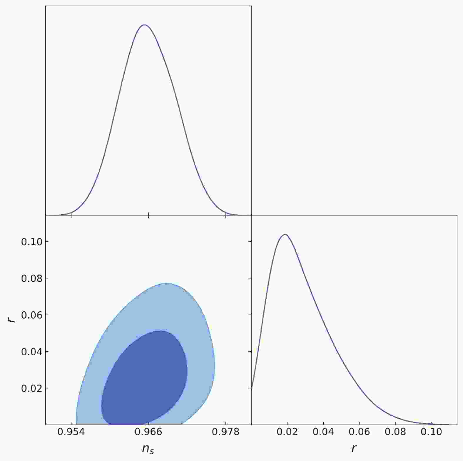
We adopt the data from P18 [27] and BK15 [30] to obtain the constraints on $ n_{s} $ and r for the $ \Lambda $CDM $ +r $ model. They are given as follows by using the Cosmomc code [34]:

The contour plots for $ n_{s} $ and r are shown in Fig. 1. The plots indicate that the power spectrum of the curvature perturbation deviates from the exact scale-invariant power spectrum at more than $ 7\sigma $ CL.

Figure 1.  (color online) The marginalized contour plots and likelihood distributions for $ n_{s} $ and r at 68%CL and 95%CL from the data of P18+BK15, respectively.

The ordinary NI potential was generalized simply by adding the parameter m in Ref. [18]. The form of potential for the GNI model is expressed as follows:

where the energy density $ \Lambda^{4} $, decay constant f, and the constant m are the parameters of the model. It follows that when $ m = 1 $, the model reduces to the NI model. If $ f\rightarrow\infty $, the NI model seems to behave like the chaotic inflationary model. Similarly, the GNI model behaves as a pure power law model when $ f\rightarrow\infty $ [18]. Fig. 2 shows the evolving tendency of the potential. The horizontal axis is $ \phi/M_{p} $, and the vertical axis is $ V(\phi)/\Lambda^{4} $. From the trajectories, we can find that if f is a fixed value, such as $ f/M_{p} = 6 $, $ V(\phi) $ changes more slowly for smaller m in the beginning, and becomes steep in the end. The trajectories reach zero at the same value of $ \phi $.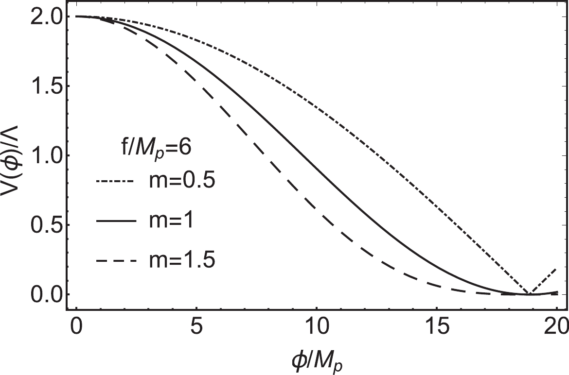

Figure 2.  The evolving trajectories of $ V(\phi) $ in the GNI model for $ m = 0.5, 1 $ and $ 1.5 $, respectively. Here, $ f/M_{p} = 6 $ is taken.

According to Eqs. (6) and (7), the slow-roll parameters $ \epsilon_{v} $ and $ \eta_{v} $ of the GNI model can be given as follows:

Thus, $ n_{s} $ and r can be expressed as:

And the e-folding number $ N_{*} $ is derived as:

When $\epsilon_{v} = \epsilon_{\rm end} = 1$, $\phi_{\rm end}$ can be obtained from Eq. (14) as follows

Substituting Eq. (19) into Eq. (18), $ \phi_{*} $ can be derived as

It follows that $ \phi_{*} $ is a function of $ (N_{*}, f, m) $. In this case, Eqs. (16) and (17) become

It can be seen that when $ m = 1 $, Eqs. (21) and (22) reduce to the results of the NI model. The predictions for $ n_{s} $ and r in the GNI model are given in Fig. 3, where $ N_{*} $ is taken in the usual range of $ [50, 60] $, and the shaded regions represent the constraints given by P18 and BK15 at 68% and 95% CL, respectively. It can be seen that the case of $ m = 1 $ (NI model) is disfavored by the data of P18 and BK15. However, the case of $ m<1 $ can provide the small values of r in the proper ranges of the values of $ n_{s} $. Thus, the GNI model is worth investigating in the case when $ m<1 $.

Figure 3.  (color online) The plots of r and $ n_{s} $ in the GNI model for $ m = 0.3, 0.5 $ and $ 1 $, respectively. $ N_{*}\in[50, 60] $ is taken and the shaded regions represent the constraints given by P18+BK15 at 68% and 95% CL, respectively.

Fig. 4 shows the allowed ranges of values of $ N_{*} $ and f when $ m = 0.3 $, $ 0.5 $ and $ 0.7 $, respectively. It can be seen that the allowable parameter space becomes large, and then becomes small with increasing m according to the areas of the shaded regions in Fig. 4. Moreover, when $ m = 0.7 $, $N_{*}^{\min} = 51.1$ can be obtained, which suggests that the minimum value of $ N_{*} $ could be larger than $ 50 $ when the value of m is relatively large. Moreover, the value of $ f/M_{p} $ is smaller than $ 10 $ in Fig. 4.

Figure 4.  (color online) Allowed ranges of values of $ N_{*} $ and f for $ m = 0.3 $, $ 0.5 $ and $ 0.7 $, respectively. In each panel, the solid curves bracket the range of values of $ n_{s} = 0.9659\pm0.0044 $, the dotted curves bracket the range of values of $ r<0.0623 $.

$ N_{*} $, $ f/M_{p} $, and m are all taken as free parameters of the GNI model, and the contour plots obtained by Cosmomc are shown in Fig. 5. It shows that the majority of the points are located in the range $ f/M_{p}<10 $, and the points corresponding to the small values of $ N_{*} $ vanish when the value of m is large. This result is consistent with our simple predictions in Fig. 4. In order to provide a direct visualization, we present the marginalized contour plots for $ f/M_{p} $ and m in the usual range $ N_{*}\in[50, 60] $ in Fig. 6. The constraints on $ f/M_{p} $ and m at 68% CL can be read as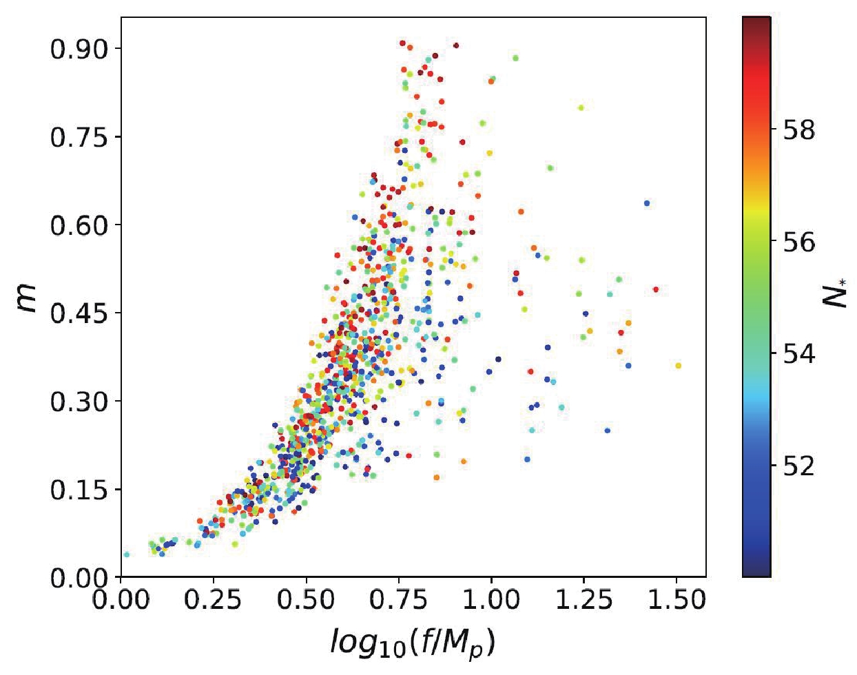

Figure 5.  (color online) The contour plots for $ N_{*} $, $ f/M_{p} $ and m in the GNI model from the data of P18+BK15, the values of $ N_{*} $ are represented by the color of the points.

Figure 6.  (color online) The marginalized contour plots for $ f/M_{p} $ and m in the GNI model at 68%CL and 95%CL from the data of P18+BK15, respectively.

Moreover, we can also calculate the higher-order slow-roll parameter $ \xi_{v}^{2} = M_{p}^{4}\dfrac{V'(\phi)V'''(\phi)}{V(\phi)^{2}} $ and the running of the scalar spectral index $\alpha_{s}\equiv \dfrac{{\rm d}n_{s}}{{\rm d}\ln k}\simeq 16\epsilon_{v}\eta_{v}- 24\epsilon_{v}^{2}- 2\xi_{v}^{2}$ of the GNI model as follows:

In Fig. 7 , we plot $ \alpha_{s} $ with respect to $ N_{*} $. The values of $ f/M_{p} $, and m are taken as the boundary values of Eqs. (23) and (24). It can be seen that $ \alpha_{s} $ is negative and, its value increases with increasing $ N_{*} $ for the fixed values of f and m. The allowable range of $ \alpha_{s} $ becomes wide with increasing m, when $ \log_{10}(f/M_{p}) = 0.62^{+0.17}_{-0.18} $, $ -0.0006\lesssim \alpha_{s}\lesssim-0.0001 $ and this can be seen in Fig. 7.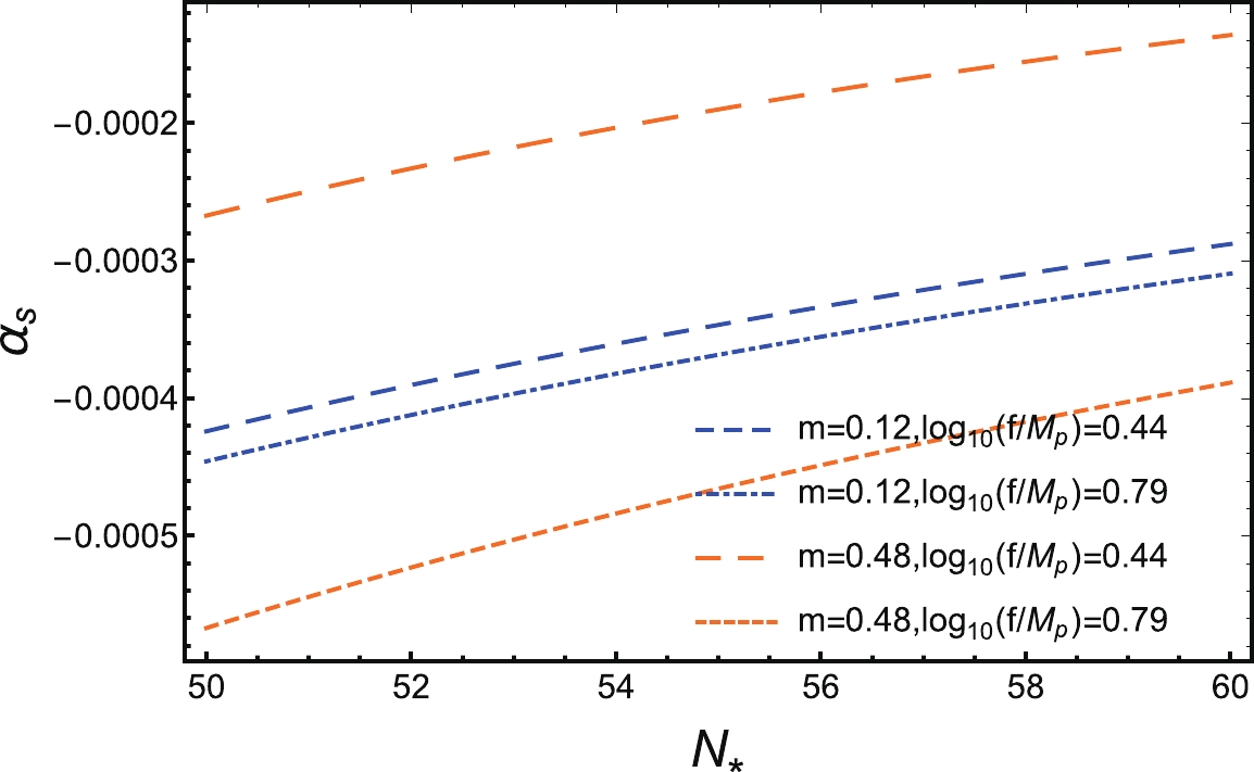

Figure 7.  (color online) The running of the scalar spectral index $ \alpha_{s} $ with respect to $ N_{*} $, the values of $ f/M_{p} $ and m are taken as the boundary values of the GNI model given by the data from P18+BK15 at 68% CL.

In addition, another important issue of the single field inflationary model is the trans-Planckian field excurison of the inflaton. This problem appears in models with large tensor-to-scalar ratio r, as indicated by the Lyth bound [39], and will spoil the basis of the effective field theory. In the GNI model considered here, r is constrained to be small, and thus, this will not be a serious problem. We plot the excursion $\Delta\phi = \mid\phi_{*}-\phi_{\rm end}\mid$ of the inflaton with respect to m in Fig. 8, and find that the excursion $ \Delta\phi $ decreases with lower m and f. One can see from Fig. 8 that with small f and m that fits the observational data, $ \Delta\phi $ might be below the Planck mass $ m_{p} = 1/\sqrt{G} = 1.2\times10^{19} $ GeV.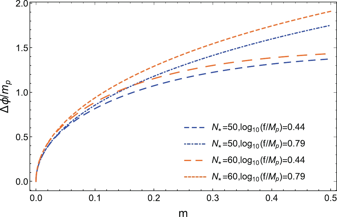

Figure 8.  (color online) The excursion $ \Delta\phi/m_{p} $ with respect to m, the values of $ N_{*} $ are taken as $ 50 $, $ 60 $, and the values of f are taken as the boundary values of the GNI model given by the data from P18+BK15 at 68% CL, respectively.

Following the approaches proposed in Refs. [36, 40, 41], the starting point for the reheating phase is $ k = aH $. This leads to:

where the subscript “${\rm re}$” corresponds to the end of reheating, $ a_{0} $ means the present value of scale factor, which is equal to $ 1 $, and the pivot scale $ k_{*} $ is chosen to be 0.05 Mpc$ ^{-1} $. Based on the conservation of the entropy density $g_{\rm re}a_{\rm re}^{3}T_{\rm re}^{3} = g_{\gamma}a_{0}^{3}T_{\gamma}^{3}+\frac{7}{8}g_{\nu}a_{0}^{3}T_{\nu}^{3}$ and the relationship of temperature $ T_{\nu}/T_{\gamma} = (4/11)^{1/3} $, the expression $ a_{re}/a_{0} $ can be written as $a_{\rm re}/a_{0} = (43/11g_{\rm re})^{1/3}/(T_{\gamma}/T_{\rm re})$, where $ T_{\gamma} = 2.7255 $ K is a known quantity. The parameter g with subscripts is the effect number of degrees of freedom, $ g_{\gamma} = 2 $ and $ g_{\nu} = 6 $, $g_{\rm re}$ is assumed as $ 10^{3} $ for single scalar field inflationary models in keeping with Planck results [25, 27, 42].

Considering the energy density of the universe at the end of reheating, $\rho_{\rm re} = g_{\rm re}\frac{\pi^{2}}{30}T_{\rm re}^{4}$, the continuity equation is $\rho_{\rm re} = \rho_{\rm end}\exp[-3(1+w_{\rm re})N_{\rm re}]$, and the expression of temperature at the end of reheating can be obtained as

where $w_{\rm re}$ is regarded as the average EoS during reheating, and $V_{\rm end}$ is used to substitute for $\rho_{\rm end}$ [42]. The relation between $V_{\rm end}$ and $\rho_{\rm end}$ can be deduced by taking $\epsilon_{H} = \dfrac{3}{2}(1+w) = \epsilon_{\rm end}$, and $\epsilon_{\rm end} = 1$ indicates the end of inflation. $ \epsilon_{H}\equiv-\dot{H}/H^{2} $ is the first Hubble hierarchy parameter, and in the slow-roll approximation, $ \epsilon_{H}\simeq\epsilon_{v} $. For a scalar field, $w\equiv P/\rho = \dfrac{\frac{1}{2}\dot{\phi}^{2}-V}{\frac{1}{2}\dot{\phi}^{2}+V}$. After a simple calculation, we can get $\rho_{\rm end}\simeq\frac{3}{2}V_{\rm end}$. Hence, the third term on the righthand side in Eq. (27) can be rewritten as $\ln\dfrac{a_{0}}{a_{\rm re}} = \dfrac{1}{3}\ln\dfrac{11g_{\rm re}}{43}- \dfrac{3}{4}(1+w_{\rm re})N_{\rm re}+\dfrac{1}{4}\ln\dfrac{45V_{\rm end}}{g_{\rm re}\pi^{2}}-\ln T_{\gamma}$. Therefore, $ H_{*} $ is the only uncertain quantity in Eq. (27), and it can be fixed by combining Eqs. (3) and (10) with the scalar amplitude $ A_{s} $ as $ A_{s}\simeq H_{*}^{2}/(\pi^{2}M_{p}^{2}r/2) $.

Finally, the expression of the e-folding number $N_{\rm re}$ during reheating can be written as follows:

For the general reheating epoch, substituting the expressions of $V_{\rm end}$ and r into Eqs. (28) and (29), $N_{\rm re}$ and $T_{\rm re}$ can be obtained for the GNI model. It is known that the EoS for the scalar field is in the range $ [-1, 1] $, and it should be smaller than $ -1/3 $ to meet the requirement of accelerated expansion. Thus, when discussing the reheating phase, the value of $ w_{\rm re} $ is usually taken in the range $-1/3\leqslant w_{\rm re}\leqslant 1$. In addition, it is easy to show that the denominator of Eq. (29) will vanish if $w_{\rm re} = 1/3$, which means $w_{\rm re} = 1/3$ is the boundary of different evolution tendencies of the reheating parameters. The evolving trajectories of the reheating e-folding number $N_{\rm re}$ and the reheating temperature $T_{\rm re}$ are illustrated in Fig. 9, three different values of $w_{\rm re}$ are considered in each panel as $w_{\rm re} = -1/3$, 0 and $ 1 $. The values of $ f/M_{p} $ and m are taken as the boundary values of Eqs. (23) and (24).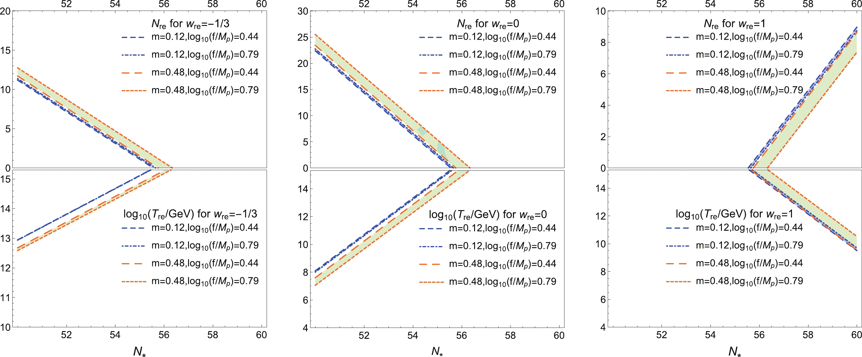

Figure 9.  (color online) The evolving trajectories of the reheating e-folding number $N_{\rm re}$ and the reheating temperature $T_{\rm re}/$ GeV with respect to $ N_{*} $ are respectively plotted in the upper and lower panels, $w_{\rm re}$ are taken as $w_{\rm re} = -1/3, 0$ and $ 1 $ in each panel from left to right, the values of $ f/M_{p} $ and m are taken as the boundary values of the GNI model given by the data from P18+BK15 at 68% CL.

It can be seen that the high limit of the reheating temperature $T_{\rm re}$ and the limits of $ N_{*} $ can be obtained by the physical condition that the reheating e-folding number $N_{\rm re}$ should be non-negative. The maximum and minimum values of $ N_{*} $ for the cases of $w_{\rm re} < 1/3$ and $w_{\rm re} > 1/3$ are respectively $N_{*}^{\max} = 56.34$ and $N_{*}^{\min} = 55.5$. Moreover, the ranges of the corresponding values of reheating parameters first increase, and then decrease with increasing $w_{\rm re}$. And we can find that $N_{\rm re}$ and $T_{\rm re}$ are slightly more sensitive to the value of m than the value of f. When $w_{\rm re} < 1/3$, $N_{\rm re}$ increases, and $T_{\rm re}$ decreases at the fixed value of m (or $ f/M_{p} $) with increasing $ f/M_{p} $ (or m). When $w_{\rm re} > 1/3$, the reheating parameters evolve in the opposite trend. The results of the corresponding ranges of values of $N_{\rm re}$ and $\log_{10}(T_{\rm re}/$GeV) for $w_{\rm re} = -1/3, 0$ and $ 1 $ in the ranges $ \log_{10}(f/M_{p}) = 0.62^{+0.17}_{-0.18} $ and $ m = 0.35^{+0.13}_{-0.23} $ are listed in Table 1.

$w_{\rm re}$	$N_{\rm re}$	$\log_{10}(T_{\rm re}/$GeV)
$ -1/3 $	$ 0-12.7 $	$ 12.6-15.3 $
$ 0 $	$ 0-25.5 $	$ 7.0-15.3 $
$ 1 $	$ 0-9.0 $	$ 9.5-15.3 $

Table 1.  The corresponding ranges of values of $N_{\rm re}$ and $\log_{10}(T_{\rm re}/$GeV) for $w_{\rm re} = -1/3$, 0 and $ 1 $ in the ranges of $ \log_{10}(f/M_{p}) = 0.62^{+0.17}_{-0.18} $ and $ m = 0.35^{+0.13}_{-0.23} $.

Here, we consider the reheating scenario as a simple case of a two-phase process. After the end of inflation, the scalar field inflaton starts to oscillate, and decays into the radiation field $ \chi $. This is the oscillatory phase. At equilibrium, the energy density of the oscillation field equals that of the relativistic particle field, i.e., the expansion Hubble constant H equals to the decay rate $ \Gamma $, the universe is dominated by radiation. Therefore, $ H = \Gamma $ is regarded as the indicator of completion of the simplest two-phase reheating. Note that, the system is not at thermal equilibrium during the process, and has gone through a process called the thermalization phase. When the $ \phi $ field oscillates around its minimum value, the potential in Eq. (13) has an approximate form $ V(\phi)\propto\phi^{2m} $. For the $ \phi^{2m} $ form-like potential, the EoS can be expressed as [36, 43]:

The reheating e-folding number $N_{\rm re}$ is reconsidered as the sum of two phases, $N_{\rm sc}$ and $N_{\rm th}$. We know that $N_{\rm sc} = \ln\dfrac{a_{\rm eq}}{a_{\rm end}}$ and $N_{\rm th} = \ln\dfrac{a_{\rm re}}{a_{\rm eq}}$, where $a_{\rm eq}$ is the dividing point of the two phases. They can be written as

and

where $w_{\rm th} = w_{r} = 1/3$ has been adopted in Eq. (32).

Based on the continuity equation, $\rho_{\rm eq}$ can be expressed as

Finally, Eqs. (31) and (32) can be rewritten as follows:

Fig. 10 shows the evolution of the oscillation e-folding number $N_{\rm sc}$ and the temperature $T_{\rm re}{\rm e}^{N_{\rm th}}/$GeV, with $ N_{*} $. We find that $N_{\rm sc}$ decreases, while $T_{\rm re}{\rm e}^{N_{\rm th}}$ increases with increasing $ N_{*} $ for the fixed values of $ f/M_{p} $ and m. Similar to the cases of the general reheating phase, $N_{\rm sc}\geqslant 0$ is required in order to make the two-phase reheating meaningful. The values of $N_{\rm sc}$ and $T_{\rm re}{\rm e}^{N_{\rm th}}/$GeV are in the ranges $ [0, 12.4] $ and $ [12.7, 15.3] $, respectively.

Figure 10.  (color online) The evolutions of $N_{\rm sc}$ and $T_{\rm re}{\rm e}^{N_{\rm th}}/$GeV with respect to $ N_{*} $ in the two-phase reheating scenario are respectively plotted in the upper and lower panels, the values of $ f/M_{p} $ and m are taken as the boundary values of the GNI model given by the data from P18+BK15 at 68% CL.

In addition, we consider the elementary decay $ \phi\rightarrow\chi\chi $ with the interaction $ -g\phi\chi^{2} $, where g respectives the coupling constant. And following Ref. [36], we take the corresponding decay rate $ \Gamma $ as $ \Gamma_{\phi\rightarrow\chi\chi} = \dfrac{g^{2}}{8\pi m_{\phi}} $, where $ m_{\phi} $ is the mass of inflaton. Considering the Friedmann equation $ H^{2} = \dfrac{\rho_{\rm eq}}{3M_{p}^{2}} $ and the equality $ H = \Gamma $, it can be directly obtained that $(\dfrac{\rho_{\rm eq}}{3M_{p}^{2}})^{1/2} = \dfrac{g^{2}}{8\pi m_{\phi}}$. Substituting Eqs. (30) and (33) into the above equation, the coupling constant g of the GNI model can be expressed as follows:

Utilizing $V_{\rm end}\sim 2^{1-m}\Lambda^{4}\left(\dfrac{mM_{p}}{f}\right)^{2m}$, the effective mass of the inflaton is $ m_{\phi}^{2}\sim m\dfrac{\Lambda^{4}}{f^{2}} $ at vacuum, and Eq. (34), g can be expressed in terms of ($ N_{*} $, f, m). Therefore, we can use the evolution of the coupling constant g to realize a successful simplest two-phase reheating scenario.

In Fig. 11, we plot the coupling constant g with respect to $ N_{*} $, the solid (red) line corresponds to $ N_{*} = 56.34 $ from the requirement $N_{\rm sc}\geqslant 0$. From Fig. 11, we find that the value of g increases with $ N_{*} $ for the fixed values of $ f/M_{p} $ and m. Moreover, it can be seen that the value of g is more sensitive to the value of m than the to value of f, and g decreases with increasing f for the fixed value of $ N_{*} $ and m. However, it decreases first, and then increases with increasing m for the fixed value of $ N_{*} $ and f, and there are turning points for $ \log_{10}(f/M_{p}) = 0.79 $ and $ 0.44 $ as $ N_{*} = 55.8 $ and $ 56.0 $, respectively. The minimum value of g to complete the two-phase reheating is in the order of magnitude of $ 10^{11} $GeV.

Figure 11.  (color onlie) The evolution trajectories of the coupling constant $ g/ $GeV with respect to $ N_{*} $, the values of $ f/M_{p} $ and m are taken as the boundary values of the GNI model given by the data from P18+BK15 at 68% CL.

In this study, we have investigated the GNI model in detail according to the latest observational data from Planck 2018 and BK15. As we discussed above, the constraints on the observable values of $ n_{s} $ and r for the $ \Lambda $CDM $ +r $ model by means of the Cosmomc code are given as $ n_{s} = 0.9659\pm0.0044 $ at 68% CL, and $ r<0.0623 $ at 95%CL (Planck TT, TE, EE+lowE+lensing+BK15).

For the GNI model, $ n_{s} $ and r have been expressed by $ N_{*} $, $ f/M_{p} $ and m, and thus, the allowable parameter space of $ (f/M_{p}, m) $ in the range $ N_{*}\in[50, 60] $ has been obtained as $ \log_{10}(f/M_{p}) = 0.62^{+0.17}_{-0.18} $ and $ m = 0.35^{+0.13}_{-0.23} $ at 68% CL. The general reheating parameters in the GNI model are functions of $ N_{*} $, f, m, and $w_{\rm re}$. Thus, we have obtained the evolutions of $N_{\rm re}$ and $\log_{10}(T_{\rm re}/$GeV) with $ N_{*} $ for $w_{\rm re} = -1/3$, 0 and $ 1 $, respectively. The corresponding ranges of the values have been shown as $N_{\rm re}\leqslant 25.5$ and $7\leqslant \log_{10}(T_{\rm re}/$GeV)$ \lesssim15 $ within the obtained allowable parameter space, when $w_{\rm re} = 0$. As for the two-phase reheating, the parameters are functions of $ N_{*} $, f and m, and the values of $N_{\rm sc}$ and $T_{\rm re}{\rm e}^{N_{\rm th}}/$GeV are in the ranges $ [0, 12.4] $ and $ [12.7, 15.3] $, respectively, and the values of the coupling constant $g/{\rm GeV}$ is in the range $11.2\leqslant\log_{10}(g/{\rm GeV})\leqslant 13.8$ within the allowable parameter space. It follows that the parameter m has significant effect on the behavior of the GNI model.

We thank Dr. Xue Zhang for helpful discussion on the Monte Carlo method.