


 Abstract
 HTML
HTML Reference
 Related
 PDF
PDF


-
$ \alpha $ -decay is one of the main decay modes of superheavy nuclei (SHN). It was first observed by Rutherford and explained as a quantum tunneling process independently by Gamow [1] and Condon and Gurney [2]. The$ \alpha $ -decay properties reflect information on the nuclear structure and nuclear stability. In experiments,$ \alpha $ -decay chains are commonly used to identify the newly synthesized SHN. To detect the “island of stability” [3-14], many SHN have been synthesized using the hot fusion reaction [15] and cold fusion reaction [16]. As the existence and stability of SHN can be mainly attributed to shell effects, it is important to evaluate the magic numbers carefully and calculate the$ \alpha $ -decay properties accurately [17-21].Many theoretical approaches have been proposed to describe the
$ \alpha $ -decay process, such as the shell model, fission-like model, and cluster model [22-25]. Many semiclassical models have been employed to reproduce the$ \alpha $ -decay half-lives, such as the generalized liquid drop model (GLDM) [26-28], Coulomb and proximity potential model (CPPM) [29], unified fission model (UFM) [30], and density-dependent cluster model (DDCM) [31]. Based on the Geiger-Nuttall law [32], many empirical relationships, such as the Viola-Seaborg formula [33, 34], Brown formula [35], Royer's formula [36], and universal decay law (UDL) [37, 38] have also been proposed to calculate the$ \alpha $ -decay half-life. These methods provide a very good description of the tunnelling of the$ \alpha $ -particle across the Coulomb barrier for heavy and super heavy nuclei. While it is difficult to describe$ \alpha $ -decay in a fully microscopic way, many works have considered microscopic modifications in the$ \alpha $ -decay calculations [39-46].In this work, we use the GLDM with shell correction, Royer's formula and UDL to calculate the
$ \alpha $ -decay half-lives of even-Z superheavy nuclei with Z = 120, 122, 124, 126. In the framework of the GLDM, two methods are adopted to calculate the$ \alpha $ -preformation factor. In the first method, the$ \alpha $ -preformation factor is considered as a constant, which is fitted from the experimental half-lives, for each type of nuclei (even-even, odd-A, odd-odd). The second method involves the use of the cluster formation model (CFM) [47-50]. We adopt the updated Weizsäcker-Skyrme-4 (WS4) model to calculate$ Q_{\alpha} $ [51], as the accuracy of the WS4 model has been generally certified [52]. To predict the decay modes, two modified shell-induced Swiatecki's formula are used to calculate the theoretical SF half-lives. One empirical relation was formulated by Santhosh and Nithya (KPS) [53, 54], while the other was modified by Bao et al. [55].This paper is structured as follows. Sec. 2 introduces the theoretical framework. The results and corresponding discussion are presented in Sec. 3. The conclusions are presented in the last section.
-
In the framework of the GLDM, the decay width is defined as
$ \lambda $ =$ P_{\alpha} $ $ \nu_{0} $ P. The Wenzel-Kramers-Brillouin (WKB) approximation is used to calculate the barrier penetrability P,$ P = \exp \left[ { - \frac{2}{h}\int\limits_{R_{\rm in} }^{R_{\rm out} } {\sqrt {2B\left( r \right)\left( {E\left( r \right) - E\left( {\rm sphere} \right)} \right)} {\rm d}r} } \right], $

(1) where
$ E_{\rm sphere} $ is the ground state energy of the parent nucleus.$ E(R_{\rm in}) $ =$ E(R_{\rm out}) $ =$ Q_{\alpha}^{\rm exp} $ ,$ B(r) $ =$ \mu $ , where the parameter$ \mu $ is the reduced mass of the daughter nucleus and$ \alpha $ -particle.$ P_{\alpha} $ is the$ \alpha $ -preformation factor, and$ \nu_{0} $ is the assault frequency that is calculated by [56]$ \nu _0 = \frac{1}{{2R}}\sqrt {\frac{{2E_\alpha }}{M_\alpha}}, $

(2) where
$ M_{\alpha} $ is the mass,$ E_{\alpha} $ is the kinetic energy of the$ \alpha $ particle that has been corrected for recoil, and R is the radius of the parent nucleus.The model considers shell correction, which is shape-dependent as defined below, [57]
$ E_{\rm shell} = E_{\rm shell}^{\rm sphere} \left( {1 - 2.6\alpha ^2 } \right){\rm e}^{ - \alpha ^2 }, $

(3) where
$ \alpha ^2 = \left( {\delta R} \right)^2 /a^2 $ is the root mean square of the deviation, which includes all types of deformation, for the particle surface from the sphere. With increase in the distortion of the nucleus, the complete shell correction energy becomes zero owing to the attenuating factor$ {\rm e}^{ - \alpha ^2 } $ .The term
$ E^{\rm sphere}_{\rm shell} $ is defined as$ E_{\rm shell}^{\rm sphere} = cE_{\rm sh}, $

(4) which represents the shell correction for a spherical nucleus.
$ E_{\rm sh} $ is the shell correction energy, which can be calculated by the Strutinsky process [58]. The Strutinsky calculations use the smoothing parameter$ \gamma = 1.2\hbar \omega _0 $ and order p = 6 of the Gauss-Hermite polynomials, where$ \hbar \omega _0 = 41A^{ - 1/3} $ is the mean distance between the gross shells. The parameter c is scaled to adapt the separation of the binding energy between the macroscopic part and microscopic correction [59]. -
The
$ \alpha $ -preformation factor$ P_{\alpha} $ is adopted from two methods. The first involves considering the same preformation factor for certain type of nuclei [60, 61]. The experimental$ P_{\alpha} $ values are extracted from nuclei with N$ \geqslant $ 152, Z$ \geqslant $ 82, a least squares fit to the experimental$ \alpha $ -decay half-lives is performed, and the$ P_{\alpha} $ values,$ P_{\alpha} $ = 0.33 (even-even),$ P_{\alpha} $ = 0.05 (odd-A), and$ P_{\alpha} $ = 0.01 (odd-odd) are obtained. These results are consistent with those extracted from the GLDM in Ref. [62].Another method to obtain the
$ \alpha $ -preformation factor involves the use of the CFM [47-50],$ P_\alpha = \frac{{E_{f\alpha } }}{E}, $

(5) where
$ E_{f\alpha} $ is the formation energy of the$ \alpha $ particle, and E is the total energy combining the intrinsic energy for the$ \alpha $ particle and the interaction energy between the$ \alpha $ particle and daughter nucleus.The energy
$ E_{f\alpha} $ is calculated from the separation energies[48, 49],$ E_{f\alpha } = \left\{ \begin{array}{l} 2S_p + 2S_n - S_c \left( {{\rm{even - even}}} \right), \\ 2S_p + S_{2n} - S_c \left( {{\rm{even - odd}}} \right), \\ S_{2p} + 2S_n - S_c \left( {{\rm{odd - even}}} \right), \\ S_{2p} + S_{2n} - S_c \left( {{\rm{odd - odd}}} \right), \\ \end{array} \right. $

(6) $ E = S_c \left( {A,Z} \right), $

(7) where
$ S_{2n} $ is the two-neutron separation energy,$ S_{2p} $ is the two-proton separation energy, and$ S_{c} $ is the$ \alpha $ -particle separation energy,$ S_{2n} \left( {A,Z} \right) = B\left( {A,Z} \right) - B\left( {A - 2,Z} \right), $

(8) $ S_{2p} \left( {A,Z} \right) = B\left( {A,Z} \right) - B\left( {A - 2,Z - 2} \right), $

(9) $ S_{c} \left( {A,Z} \right) = B\left( {A,Z} \right) - B\left( {A - 4,Z - 2} \right), $

(10) where B is the binding energy. The binding energy can be calculated from the nucleus excess mass
$ \Delta M $ . Hence,$ S_{2p} $ ,$ S_{2n} $ , and$ S_{c} $ can be written as,$ S_{2p} \left( {A,Z} \right) = \Delta M\left( {A - 2,Z - 2} \right) - \Delta M\left( {A,Z} \right) + 2\Delta M_p , $

(11) $ S_{2n} \left( {A,Z} \right) = \Delta M\left( {A - 2,Z} \right) - \Delta M\left( {A,Z} \right) + 2\Delta M_n , $

(12) $ S_c \left( {A,Z} \right) = \Delta M\left( {A - 4,Z - 2} \right) - \Delta M\left( {A,Z} \right) + 2\Delta M_p + 2\Delta M_n . $

(13) -
Royer's formula fits different types of nuclei to calculate the
$ \alpha $ -decay half-lives [36]. For even-even nuclei, this formula fits 131 even-even nuclei, with a root mean square (RMS) deviation of 0.285,$ \log _{10} [T_{1/2} ({\rm s})] = - 25.31 - 1.1629A^{1/6} Z^{1/2} + 1.5864Z/\sqrt {Q_\alpha }. $

(14) For the subset of 106 even-odd nuclei, the following equation was obtained (RMS deviation = 0.39),
$ \log _{10} [T_{1/2} ({\rm s})] = - 26.65 - 1.0859A^{1/6} Z^{1/2} + 1.5848Z/\sqrt {Q_\alpha }. $

(15) For odd-even nuclei, 86 nuclei were adopted with a RMS deviation of 0.36,
$ \log _{10} [T_{1/2} ({\rm s})] = - 25.68 - 1.1423A^{1/6} Z^{1/2} + 1.592Z/\sqrt {Q_\alpha }. $

(16) For odd-odd nuclei, 50 nuclei were used (RMS deviation = 0.35),
$ \log _{10} [T_{1/2} ({\rm s})] = - 29.48 - 1.113A^{1/6} Z^{1/2} + 1.6971Z/\sqrt {Q_\alpha }. $

(17) The UDL were also adopted to calculate the
$ \alpha $ -decay half-lives [37, 38],$ \log _{10} [T_{1/2} ({\rm s})] = aZ_\alpha Z_d \sqrt {\frac{A}{{Q_\alpha }}} + b\sqrt {AZ_\alpha Z_d \left( {A_d^{1/3} + A_\alpha ^{1/3} } \right)} + c, $

(18) where
$ A = \frac{{A_d A_\alpha }}{{A_d + A_\alpha }} $ , a=0.4314, b=−0.4087, and c=−25.7725, which can be determined from the experimental data. -
The spontaneous fission half-lives are calculated using semi-empirical formulas based on the Swiatecki formula [63]. One formula was modified by Santhosh and Nithya [54] (KPS), while the other was reported by Bao et al. [55]. Both empirical relations considered the isospin effect (
$ \frac{{N - Z}}{{N + Z}} $ ), fissionability parameter ($ \frac{{Z^2 }}{A} $ ) , and shell effect [53-55, 64].The KPS formula is defined as follows [53, 54],
$ \begin{split} {\log _{10}}\left( {{T_{1/2}}{(\rm yr)}} \right) =& a\frac{{{Z^2}}}{A} + b{\left( {\frac{{{Z^2}}}{A}} \right)^2} + c\left( {\frac{{N - Z}}{{N + Z}}} \right)\\ &+ d{\left( {\frac{{N - Z}}{{N + Z}}} \right)^2} + e{E_{\rm shell}} + f, \end{split}$

(19) where a = −43.25203, b = 0.49192, c = 3674.3927, d = −9360.6, e = 0.8930, and f = 578.56058.
$ E_{\rm shell} $ is the shell correction energy from the FRDM [65].The modified empirical formula reported by Bao et al. is determined as follows [55],
$ \begin{split} \log _{10} [T_{1/2} ({\rm yr})] =& c_1 + c_2 \left( {\frac{{Z^2 }}{{\left( {1 - kI^2 } \right)A}}} \right)\\& + c_3 \left( {\frac{{Z^2 }}{{\left( {1 - kI^2 } \right)A}}} \right)^2 + c_4 E_{\rm sh} + h_i, \end{split} $

(20) where
$ Z^{2}/(1 - kI^{2})A $ is the fissionability parameter considering the isospin effect. The constant k = 2.6 [36]. The coefficients$ c_1 $ = 1174.353441,$ c_2 $ = −47.666855,$ c_3 $ = 0.471307, and$ c_4 $ = 3.378848, which were fitted from 45 even-even nuclei. The blocking effect is also considered by parameter$ h_{i} $ , where$ h_{\rm eo} $ = 2.609374 (even-odd),$ h_{\rm oe} $ = 2.619768 (odd-even),$ h_{\rm oo} $ =$ h_{\rm eo} $ +$ h_{\rm oe} $ (odd-odd), and$ h_{\rm ee} $ = 0 (even-even). The shell correction energy$ E_{\rm sh} $ is derived from Ref. [65]. -
Table 1 presents the
$ \alpha $ -decay half-lives of known nuclei from Fl to Og calculated with the GLDM, UDL, and Royer's formula. These nuclei are regarded as the “upper super heavy region” [66] and are produced by hot-fusion reactions. The$ P_{\alpha} $ adopted in the GLDM is obtained via a least squares fit to the experimental half-lives for known SHN from N$ \geqslant $ 152 and Z$ \geqslant $ 82. The experimental$ Q_{\alpha} $ values are derived from Ref. [67]. The standard deviation was used to compare the calculation results and experimental values,Ele. A $Q_{\alpha}^{\rm exp.}$ /MeV

$T_{1/2}^{\rm exp.}$ /s

$T_{1/2}$ /s

$T_{1/2}$ /s

$T_{1/2}$ /s

$T_{1/2}$ /s

Royer UDL GLDM GLDM $_{\rm shell}$ 

Fl 285 10.56 $\pm$ 0.05

1.00 $\times$ 10

$^{-1 }$ 

1.60 $\times$ 10

$^{-1 }$ 

4.27 $\times$ 10

$^{-2 }$ 

6.61 $\times$ 10

$^{-2 }$ 

6.57 $\times$ 10

$^{-2 }$ 

286 10.35 $\pm$ 0.04

1.20 $\times$ 10

$^{-1 }$ 

1.08 $\times$ 10

$^{-1 }$ 

1.62 $\times$ 10

$^{-1 }$ 

3.16 $\times$ 10

$^{-2 }$ 

3.37 $\times$ 10

$^{-2 }$ 

287 10.17 $\pm$ 0.02

4.80 $\times$ 10

$^{-1 }$ 

1.68 $\times$ 10

$^{0 }$ 

5.25 $\times$ 10

$^{-1 }$ 

5.67 $\times$ 10

$^{-1 }$ 

6.67 $\times$ 10

$^{-1 }$ 

288 10.07 $\pm$ 0.03

6.60 $\times$ 10

$^{-1 }$ 

5.93 $\times$ 10

$^{-1 }$ 

1.01 $\times$ 10

$^{0 }$ 

1.47 $\times$ 10

$^{-1 }$ 

1.99 $\times$ 10

$^{-1 }$ 

289 9.98 $\pm$ 0.02

1.90 $\times$ 10

$^{0 }$ 

5.34 $\times$ 10

$^{0 }$ 

1.82 $\times$ 10

$^{0 }$ 

1.60 $\times$ 10

$^{0 }$ 

2.55 $\times$ 10

$^{0 }$ 

Mc 287 10.76 $\pm$ 0.05

3.70 $\times$ 10

$^{-2 }$ 

4.70 $\times$ 10

$^{-2 }$ 

2.60 $\times$ 10

$^{-2 }$ 

4.06 $\times$ 10

$^{-2 }$ 

3.85 $\times$ 10

$^{-2 }$ 

288 10.65 $\pm$ 0.01

1.74 $\times$ 10

$^{-1 }$ 

4.49 $\times$ 10

$^{-1 }$ 

5.05 $\times$ 10

$^{-2 }$ 

3.57 $\times$ 10

$^{-1 }$ 

3.47 $\times$ 10

$^{-1 }$ 

289 10.49 $\pm$ 0.05

3.30 $\times$ 10

$^{-1 }$ 

2.23 $\times$ 10

$^{-1 }$ 

1.37 $\times$ 10

$^{-1 }$ 

1.67 $\times$ 10

$^{-1 }$ 

1.82 $\times$ 10

$^{-1 }$ 

290 10.41 $\pm$ 0.04

6.50 $\times$ 10

$^{-1 }$ 

2.00 $\times$ 10

$^{0 }$ 

2.25 $\times$ 10

$^{-1 }$ 

1.26 $\times$ 10

$^{0 }$ 

1.51 $\times$ 10

$^{0 }$ 

Lv 290 11 $\pm$ 0.07

8.30 $\times$ 10

$^{-3 }$ 

8.94 $\times$ 10

$^{-3 }$ 

1.21 $\times$ 10

$^{-2 }$ 

3.00 $\times$ 10

$^{-3 }$ 

2.88 $\times$ 10

$^{-3 }$ 

291 10.89 $\pm$ 0.07

1.90 $\times$ 10

$^{-2 }$ 

8.94 $\times$ 10

$^{-2 }$ 

2.31 $\times$ 10

$^{-2 }$ 

3.41 $\times$ 10

$^{-2 }$ 

3.51 $\times$ 10

$^{-2 }$ 

292 10.78 $\pm$ 0.02

1.30 $\times$ 10

$^{-2 }$ 

3.01 $\times$ 10

$^{-2 }$ 

4.46 $\times$ 10

$^{-2 }$ 

8.84 $\times$ 10

$^{-3 }$ 

1.04 $\times$ 10

$^{-2 }$ 

293 10.71 $\pm$ 0.02

5.70 $\times$ 10

$^{-2 }$ 

2.41 $\times$ 10

$^{-1 }$ 

6.72 $\times$ 10

$^{-2 }$ 

8.01 $\times$ 10

$^{-2 }$ 

1.04 $\times$ 10

$^{-1 }$ 

Ts 293 11.32 $\pm$ 0.05

2.20 $\times$ 10

$^{-2 }$ 

6.89 $\times$ 10

$^{-3 }$ 

3.57 $\times$ 10

$^{-3 }$ 

6.59 $\times$ 10

$^{-3 }$ 

6.65 $\times$ 10

$^{-3 }$ 

294 11.18 $\pm$ 0.04

5.10 $\times$ 10

$^{-2 }$ 

7.25 $\times$ 10

$^{-2 }$ 

7.98 $\times$ 10

$^{-3 }$ 

6.45 $\times$ 10

$^{-2 }$ 

7.23 $\times$ 10

$^{-2 }$ 

Og 294 11.82 $\pm$ 0.06

5.80 $\times$ 10

$^{-4 }$ 

3.67 $\times$ 10

$^{-4 }$ 

4.26 $\times$ 10

$^{-4 }$ 

1.64 $\times$ 10

$^{-4 }$ 

1.60 $\times$ 10

$^{-4 }$ 

0.38 0.39 0.35 0.35 Table 1. Experimental and theoretical
$\alpha$ -decay half-lives of known SHN from Fl to Og. The theoretical results are calculated using Royer's formula, the UDL, and the GLDM with and without shell corrections by inputting the experimental$Q_{\alpha}$ [67]. The$P_{\alpha}$ adopted in the GLDM is a constant, which is fitted from the experimental data ($P_{\alpha}$ = 0.33 for even-even nuclei,$P_{\alpha}$ = 0.05 for odd-A nuclei, and$P_{\alpha}$ = 0.01 for odd-odd nuclei). Here,$\sigma$ represents the standard deviation between the experimental results and theoretical calculations obtained with Eq. (21).$ \sigma {\rm{ = }}\left[ {\frac{1}{{n - 1}}\sum\limits_{i = 1}^n {\left( {\log _{10} T_{1/2}^{\rm theo.} - \log _{10} T_{1/2}^{\exp .} } \right)^2 } } \right]^{1/2} . $

(21) The
$ \sigma $ values of Royer's formula, the UDL, the GLDM, and GLDM with shell correction are 0.38, 0.39, 0.35, and 0.35, respectively. The effect of shell correction is more obvious for nuclei near the predicted shell-closure [68]. For example, considering$ ^{289} $ Fl,$ T_{\alpha}^{1/2} $ increases from 0.32 s to 0.51 s.The results obtained with the GLDM are systematically lower than the experimental data. After shell correction, the calculated
$ \alpha $ -decay half-lives increase slightly. The$ \sigma $ values indicate that using the experimentally fitted constant$ P_{\alpha} $ , the models with and without shell correction can all accurately calculate the$ \alpha $ -decay half-lives. -
The
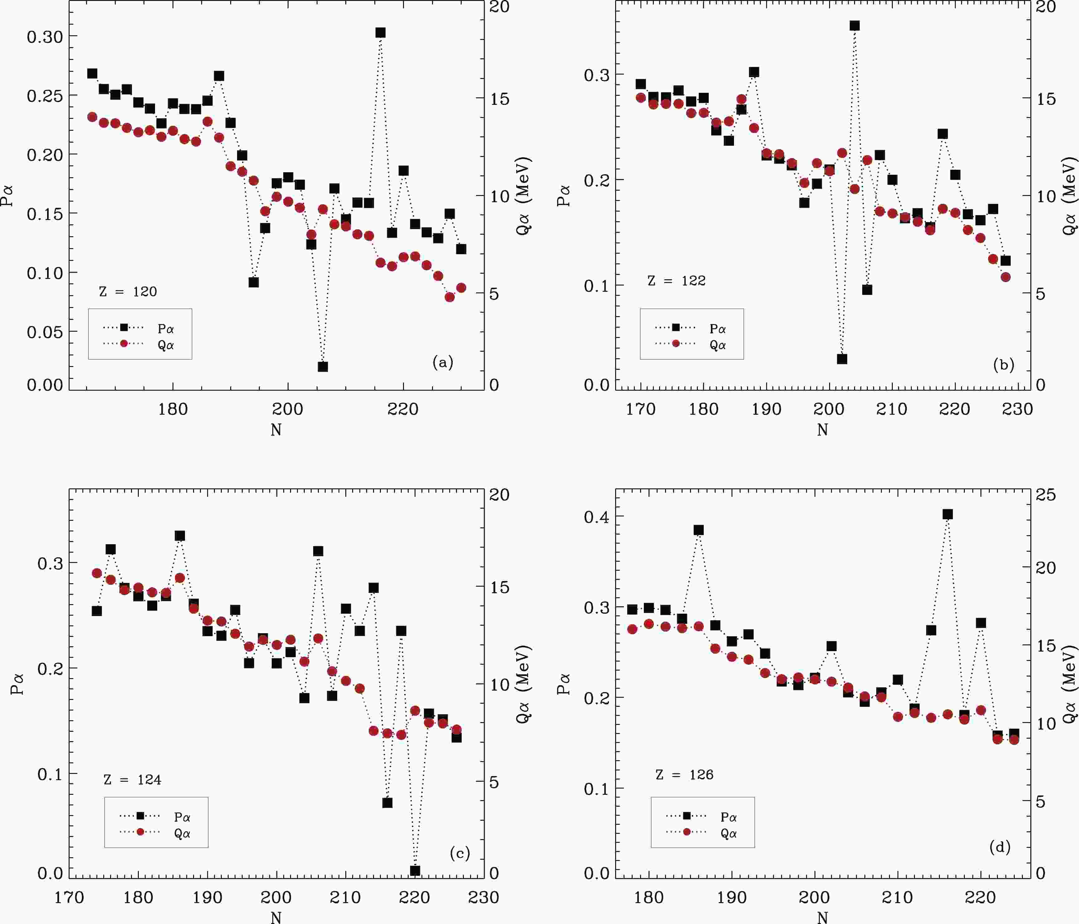
$ \alpha $ -preformation factors are calculated using the CFM [48, 49]. Both$ Q_{\alpha} $ and$ P_{\alpha} $ are extracted from the WS4 model [51]. The$ Q_{\alpha} $ and$ P_{\alpha} $ values of even-even nuclei from Z = 120 to 126 are plotted in Fig. 1. The$ P_{\alpha} $ values of even-even nuclei are approximately 0.1–0.3, which satisfies the general experimental features [49, 69]. The figure shows that the$ Q_{\alpha} $ values decrease with larger neutron numbers, indicating an increase in the stability of the nucleus against$ \alpha $ -decay. Both$ Q_{\alpha} $ and$ P_{\alpha} $ exhibit very similar trends.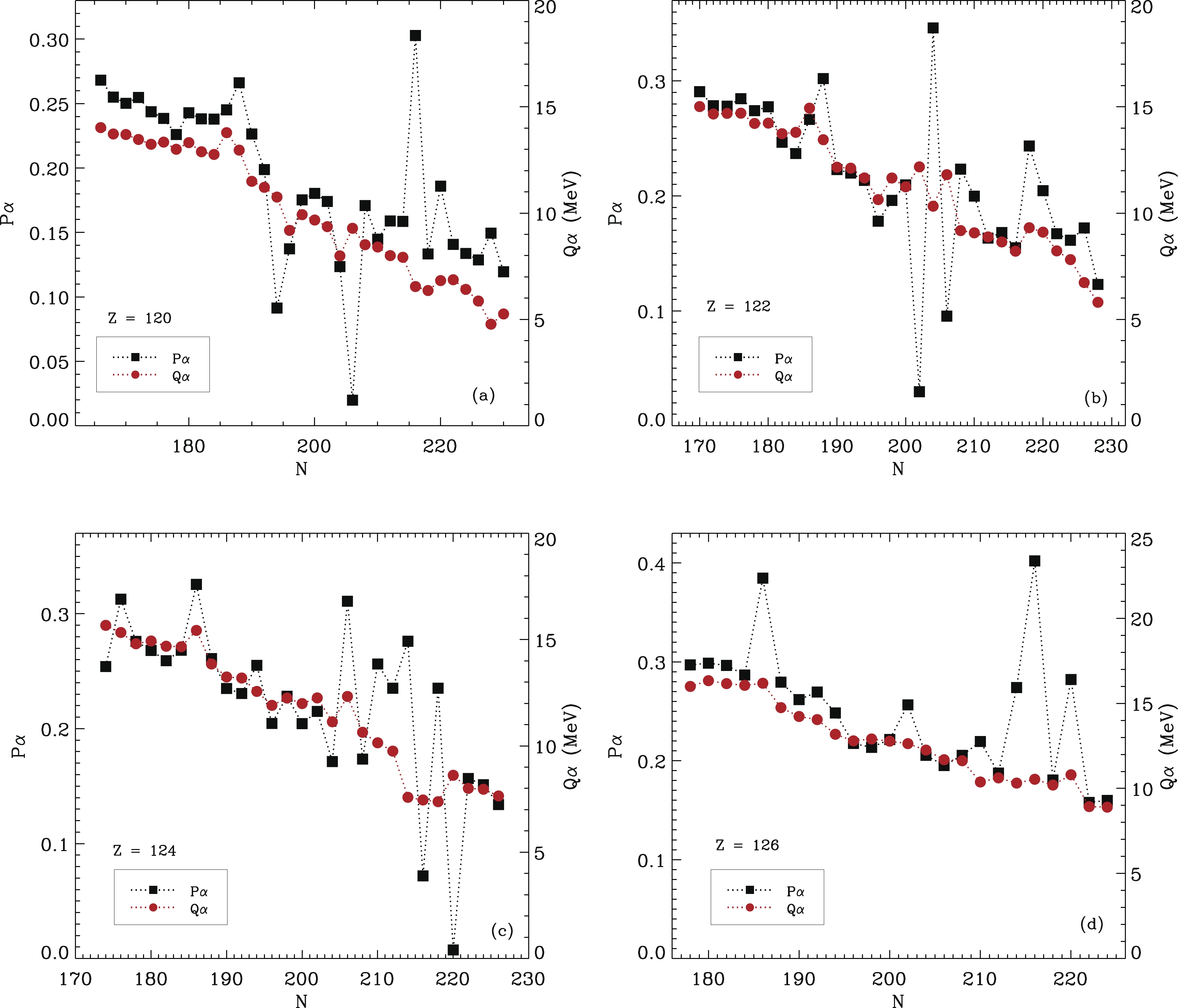
Figure 1. (color online) Preformation factors of Z = 120, 122, 124, 126 even-even nuclei.
The discontinuity of
$ Q_{\alpha} $ represents the position of the magic numbers. Moreover, in the region where the$ P_{\alpha} $ value is relatively small, the nuclei are regarded to be stable [70]. However the positions of the$ P_{\alpha} $ discontinuity and$ Q_{\alpha} $ discontinuity are not particularly the same, as shown in the case of Z = 120 even-even isotopes in Fig. 1(a). This is because the$ P_{\alpha} $ value of one nucleus is calculated based on five nuclei around it. The$ P_{\alpha} $ values may contain the complex structure information of several nearby nuclei.We use the
$ Q_{\alpha} $ and$ P_{\alpha} $ values to predict the stable nuclei for Z = 122 – 126 elements. Figure 1(a) shows that for Z = 120, the nuclei around N = 178, 184, 194, 196, 204, 206, 218, 228 might be stable. For Z = 122, the nuclei with N = 182, 184, 196, 202, 206, 216 show higher stability. For Z = 124 nuclei, the nuclei with N = 204, 208, 216, 220 might be stable against$ \alpha $ -decay. Figure 1(d) indicates that Z = 126 even-even nuclei have no obvious shell structures. This is because the$ Q_{\alpha} $ of Z = 126 isotopes are smoothly continuous, and the$ P_{\alpha} $ distribution has no dips. It can be observed that when the atomic number increases, the neutron numbers of stable nuclei also increase. It appears that with larger proton numbers, the nucleus requires more neutrons to remain stable. -
Figure 2 presents the
$ \alpha $ -decay half-lives of Z = 120, 122, 124, 126 even-even isotopes. This figure shows that at N$ < $ 186, the$ \alpha $ -decay half-lives increase with increasing nuclear mass. This phenomenon indicates that this might correspond to a shell closure at N$ < $ 186. For Z = 120 nuclei, there is one obvious peak at N = 184. However, this peak gradually disappears with increase in the Z values. The$ \alpha $ -decay half-lives indicate that the neutron magic number at N = 184 is not observed at Z = 122, 124, 126. This phenomenon is consistent with the results shown by$ P_{\alpha} $ and$ Q_{\alpha} $ in Fig. 1. For Z = 122, nuclei with N = 182 and 184 both have relatively longer half-lives, as shown in Fig. 2(b). The corresponding$ Q_{\alpha} $ and$ P_{\alpha} $ values in Fig. 1(b) are relatively small. Hence, for element Z = 120, 122, 124, 126 isotopes,$ ^{304} $ 120 would probably be stable and might be a shell closure.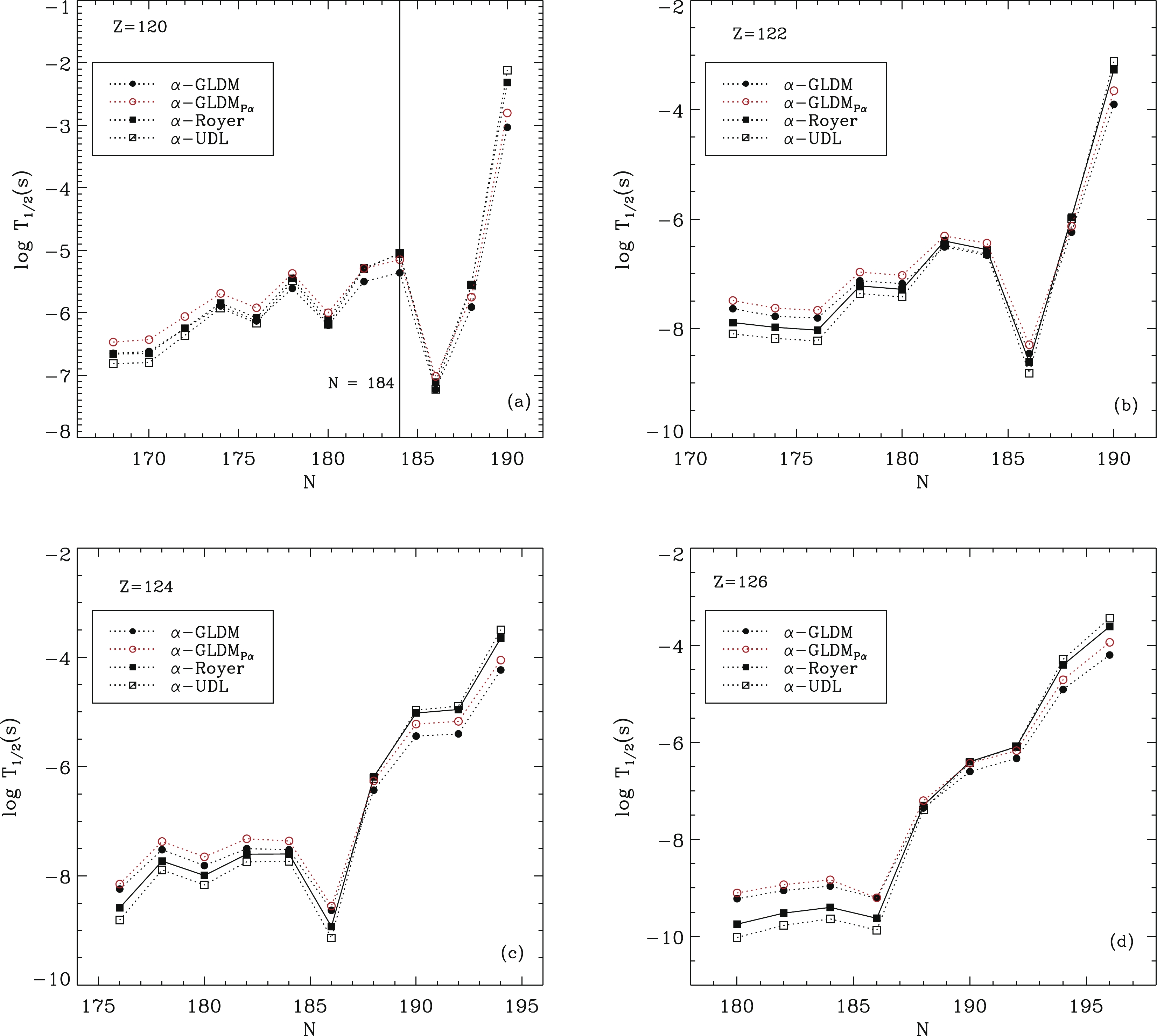
Figure 2. (color online) The
$ \alpha $ -decay half-lives of even-even isotopes of Z = 120, 122, 124, 126.The
$ \alpha $ -decay half-lives and SF half-lives of$ ^{287-339} $ 120,$ ^{294-339} $ 122,$ ^{300-339} $ 124, and$ ^{306-339} $ 126 are presented in Table 2. To identify the decay modes of unknown nuclei, the competition between$ \alpha $ -decay and spontaneous fission was studied [71-77]. The predicted decay modes of nuclei are presented in the last column of Table 2. Both SF equations consider the shell correction. However, the SF half-lives calculated with Eq. (20) would be more sensitive to the nuclear structures [78]. The results show that most nuclei at around N = 184 would undergo$ \alpha $ -decay. With a larger Z, the competition between$ \alpha $ -decay and SF would be more obvious. By comparing the$ \alpha $ -decay and SF half-lives, we predict that$ ^{287-307} $ 120 would undergo$ \alpha $ -decay,$ ^{308-309} $ 120 would undergo both$ \alpha $ -decay and SF, and$ ^{310-339} $ 120 would experience SF. The$ ^{294-309} $ 122 isotopes would undergo$ \alpha $ -decay,$ ^{310-314} $ 122 would have two decay modes, and$ ^{315-339} $ 122 would experience SF. For Z = 124 nuclei,$ ^{300-315} $ 124 would have$ \alpha $ -decay,$ ^{316-320,326,327,331} $ 124 would have both$ \alpha $ -decay and SF, and$ ^{321-325,328-330,332-339} $ 124 would undergo SF. As the competition between the two decay modes for the$ ^{328-339} $ 126 isotopes is very obvious,$ ^{328-335,337,339} $ 126 would experience both$ \alpha $ -decay and SF,$ ^{336,338} $ 126 would undergo SF, and$ ^{306-327} $ 126 would undergo$ \alpha $ -decay.Z A $Q_{\alpha}^{\rm WS4}$ /MeV

$T_{1/2}^{\alpha}\;/{\rm s}$ 

$T_{1/2}^{\alpha}\;/{\rm s}$ 

$T_{1/2}^{\alpha}\;/{\rm s}$ 

$T_{1/2}^{\alpha}\;/{\rm s}$ 

$T_{1/2}^{\rm SF}\;/{\rm s}$ 

$T_{1/2}^{\rm SF}\;/{\rm s}$ 

Decay mode Royer UDL GLDM GLDM $_{P_{\alpha}}$ 

Eq. (20) [55] KPS [54] 120 287 13.85 7.90E-07 8.96E-08 1.12E-06 4.46E-07 3.39E+03 1.03E+10 $\alpha$ 

288 13.73 2.18E-07 1.53E-07 2.62E-07 3.39E-07 1.68E+01 5.83E+10 $\alpha$ 

289 13.71 1.31E-06 1.55E-07 1.79E-06 7.17E-07 1.70E+05 4.73E+11 $\alpha$ 

290 13.70 2.23E-07 1.59E-07 2.82E-07 3.72E-07 3.45E+02 1.16E+12 $\alpha$ 

291 13.51 2.96E-06 3.73E-07 3.75E-06 1.50E-06 5.63E+05 3.19E+12 $\alpha$ 

292 13.47 5.65E-07 4.36E-07 6.66E-07 8.62E-07 1.76E+03 4.86E+12 $\alpha$ 

293 13.40 4.41E-06 5.77E-07 5.28E-06 2.26E-06 1.65E+07 1.20E+13 $\alpha$ 

294 13.24 1.43E-06 1.19E-06 1.52E-06 2.06E-06 4.25E+04 9.94E+12 $\alpha$ 

295 13.27 7.26E-06 9.91E-07 7.85E-06 3.29E-06 1.50E+08 1.10E+13 $\alpha$ 

296 13.34 8.30E-07 6.79E-07 8.70E-07 1.20E-06 2.84E+04 2.66E+12 $\alpha$ 

297 13.14 1.21E-05 1.72E-06 1.15E-05 5.32E-06 2.37E+07 1.18E+12 $\alpha$ 

298 13.01 3.56E-06 3.24E-06 2.90E-06 4.24E-06 6.02E+04 3.40E+11 $\alpha$ 

299 13.26 6.56E-06 9.08E-07 6.53E-06 2.72E-06 2.58E+07 7.66E+10 $\alpha$ 

300 13.32 7.82E-07 6.59E-07 7.40E-07 1.01E-06 3.80E+03 6.33E+09 $\alpha$ 

301 13.06 1.48E-05 2.18E-06 1.23E-05 5.16E-06 1.67E+06 8.84E+08 $\alpha$ 

302 12.89 5.21E-06 5.02E-06 3.73E-06 5.17E-06 1.17E+02 3.73E+07 $\alpha$ 

303 12.81 4.53E-05 7.25E-06 3.15E-05 1.25E-05 3.32E+04 2.91E+06 $\alpha$ 

304 12.76 8.79E-06 8.89E-06 5.13E-06 7.12E-06 5.87E-01 5.42E+04 $\alpha$ 

305 13.28 4.74E-06 6.64E-07 3.56E-06 1.45E-06 3.40E-01 5.27E+02 $\alpha$ 

306 13.79 7.76E-08 5.94E-08 7.03E-08 9.47E-08 2.24E-06 4.88E+00 $\alpha$ 

307 13.52 1.48E-06 1.94E-07 1.15E-06 4.72E-07 6.53E-05 8.70E-02 $\alpha$ 

308 12.97 2.84E-06 2.76E-06 1.44E-06 1.78E-06 3.20E-08 1.65E-03 $\alpha$ /SF

309 12.16 9.06E-04 1.81E-04 2.97E-04 1.09E-04 9.87E-06 3.64E-05 $\alpha$ /SF

310 11.50 4.88E-03 7.72E-03 1.10E-03 1.60E-03 1.32E-09 3.28E-07 SF 311 11.20 1.68E-01 4.73E-02 3.47E-02 1.71E-02 2.43E-07 4.25E-09 SF 312 11.22 2.27E-02 4.02E-02 4.20E-03 6.97E-03 1.79E-11 2.22E-11 SF 313 11.02 4.26E-01 1.29E-01 7.60E-02 3.96E-02 5.39E-09 2.24E-13 SF 314 10.76 3.29E-01 6.99E-01 4.84E-02 1.75E-01 5.15E-13 8.66E-16 SF 315 9.43 1.73E+04 1.04E+04 7.27E+03 3.99E+03 1.86E-10 6.38E-18 SF 316 9.19 1.71E+04 7.33E+04 8.70E+03 2.09E+04 3.41E-14 2.04E-20 SF 317 9.93 4.26E+02 2.05E+02 1.28E+02 7.12E+01 7.92E-12 9.44E-23 SF 318 9.93 6.57E+01 2.01E+02 1.88E+01 3.53E+01 1.74E-15 2.26E-25 SF 319 9.84 7.35E+02 3.70E+02 2.20E+02 1.28E+02 4.86E-13 7.81E-28 SF 320 9.68 3.68E+02 1.28E+03 1.18E+02 2.16E+02 1.75E-16 1.53E-30 SF 321 9.53 6.77E+03 3.97E+03 2.34E+03 1.36E+03 3.02E-13 6.21E-33 SF 322 9.37 3.44E+03 1.40E+04 1.28E+03 2.42E+03 1.12E-16 8.92E-36 SF 323 9.12 1.48E+05 1.07E+05 6.75E+04 3.73E+04 6.68E-14 2.01E-38 SF Continued on next page Table 2. Theoretical
$\alpha$ -decay half-lives and SF half-lives of the$^{287-339}$ 120,$^{294-339}$ 122,$^{300-339}$ 124, and$^{306-339}$ 126 isotopes. The$Q_{\alpha}^{\rm th.}$ values are extracted from the WS4 model [51]. Columns (4-7) present the$\alpha$ -decay half-lives calculated using Royer's formula, the UDL, the GLDM with shell correction, and the GLDM with shell correction and CFM$P_{\alpha}$ , respectively. Columns (8-9) present the SF half-lives calculated using Eq. (20) [55] and the KPS equation [54], respectively. The last column lists the predicted decay modes.In addition, the FRDM
$ Q_{\alpha} $ values are used to calculate the$ \alpha $ -decay half-lives, and the results are shown in Table 3. For Z = 120 isotopes,$ ^{296-307} $ 120 would undergo$ \alpha $ -decay,$ ^{308} $ 120 may undergo both$ \alpha $ -decay and SF, and$ ^{309-327} $ 120 would experience SF. For Z = 122 nuclei,$ ^{300-309,311} $ 122 would probably undergo$ \alpha $ -decay,$ ^{310,312-315} $ 122 may exhibit both decay modes, and$ ^{316-331} $ 122 experience SF. The$ ^{304-315,317} $ 124 isotopes probably undergo$ \alpha $ -decay,$ ^{316,318-320,327} $ 124 have both$ \alpha $ -decay and SF, and$ ^{321-335} $ 124 would undergo SF. For Z = 126,$ ^{308-322,325} $ 126 may experience$ \alpha $ -decay,$ ^{323,326-335,337,339} $ 126 would probably exhibit two decay modes, and$ ^{324,336,338} $ 126 would exhibit the SF decay mode. As the adopted$ Q_{\alpha} $ values are different in Table 2 and Table 3, the theoretical$ \alpha $ -decay half-lives are slightly different. However, the predicted decay modes from the two sets of results are mostly similar. Both the FRDM and WS4 models are capable of providing accurate$ Q_{\alpha} $ values for the$ \alpha $ -decay calculations.Z A $Q_{\alpha}^{\rm FRDM}$ /MeV

$T_{1/2}^{\alpha}\;/{\rm s}$ 

$T_{1/2}^{\alpha}\;/{\rm s}$ 

$T_{1/2}^{\rm SF}\;/{\rm s}$ 

$T_{1/2}^{\rm SF}\;/{\rm s}$ 

Decay mode GLDM GLDM $_{P_{\alpha}}$ 

Eq. (20) [55] KPS [54] 120 296 13.59 3.80E-07 7.40E-07 2.84E+04 2.66E+12 $\alpha$ 

297 13.65 1.99E-06 1.30E-06 2.37E+07 1.18E+12 $\alpha$ 

298 13.24 1.42E-06 2.43E-06 6.02E+04 3.40E+11 $\alpha$ 

299 13.74 1.31E-06 5.87E-07 2.58E+07 7.66E+10 $\alpha$ 

300 13.69 2.20E-07 3.75E-07 3.80E+03 6.33E+09 $\alpha$ 

301 13.62 1.83E-06 1.01E-06 1.67E+06 8.84E+08 $\alpha$ 

302 13.56 3.18E-07 5.64E-07 1.17E+02 3.73E+07 $\alpha$ 

303 13.52 2.23E-06 1.24E-06 3.32E+04 2.91E+06 $\alpha$ 

304 13.55 2.38E-07 4.41E-07 5.87E-01 5.42E+04 $\alpha$ 

305 14.26 1.16E-07 5.92E-08 3.40E-01 5.27E+02 $\alpha$ 

306 14.27 1.49E-08 2.06E-08 2.24E-06 4.88E+00 $\alpha$ 

307 13.62 8.93E-07 2.30E-07 6.53E-05 8.70E-02 $\alpha$ 

308 12.97 1.58E-06 1.58E-06 3.20E-08 1.65E-03 $\alpha$ /SF

309 11.76 2.43E-03 8.53E-04 9.87E-06 3.64E-05 SF 310 11.28 4.18E-03 7.11E-03 1.32E-09 3.28E-07 SF 311 10.76 5.08E-01 3.32E-01 2.43E-07 4.25E-09 SF 312 10.71 9.12E-02 1.87E-01 1.79E-11 2.22E-11 SF 313 10.50 2.09E+00 1.33E+00 5.39E-09 2.24E-13 SF Continued on next page Table 3. Theoretical
$\alpha$ -decay half-lives and SF half-lives of the$^{296-327}$ 120,$^{300-331}$ 122,$^{304-335}$ 124, and$^{308-339}$ 126 isotopes. The$Q_{\alpha}^{\rm th.}$ values are extracted from the FRDM [65]. Columns (4-5) present the$\alpha$ -decay half-lives calculated with the GLDM with shell correction, and the GLDM with shell correction and CFM$P_{\alpha}$ . Columns (6,7) present the SF half-lives calculated using Eq. (20) [55] and the KPS equation [54], respectively. The last column lists the predicted decay modes. -
We compare our results with those calculated with phenomenological models [78, 79]. For the
$ \alpha $ -decay half-lives obtained using the FRDM$ Q_{\alpha} $ values, we compare our results with those reported in Ref. [78]. The$ \alpha $ -decay and SF half-lives are shown in Fig. 3. The results show that the SF half-lives calculated with the modified equation reported by Bao et al. [55, 78] have an even-odd effect. This is because in Eq. (20), the blocking effect of the unpaired nucleon has been considered. The SF half-lives show a trend where with increasing A, the$ \log_{10} $ $ T_{1/2}^{\rm SF} $ values decrease. It appears that the SF equation modified by Refs. [55, 78] is more sensitive to the nuclear strucure [78]. The$ \alpha $ -decay half-lives and SF half-lives reported in this work and Ref. [78] are slightly different. This is because we use FRDM2016 [65] to calculate the$ Q_{\alpha} $ and shell correction, whereas the results from Ref. [78] are based on FRDM1995 [80]. However, the predicted decay modes for most nuclei are the same.
Figure 3. (color online) The
$ \alpha $ -decay half-lives and SF half-lives of$ ^{296-308} $ 120,$ ^{300-310} $ 122, and$ ^{304-312} $ 124. The$ \log_{10} $ $ T_{1/2}^{\alpha} $ values calculated using the UDL and GLDM are derived from Ref. [78].We compare the
$ \alpha $ -decay half-lives calculated with the WS4$ Q_{\alpha} $ values with the results from Ref. [79]. The$ \alpha $ -decay half-lives from this work and Ref. [79] are presented in Fig. 4. The$ \log_{10} $ $ T_{1/2}^{\alpha} $ values obtained using the Coulomb and proximity potential model for deformed nuclei (CPPMDN) and Coulomb and proximity potential model (CPPM) are from Ref. [79]. The SF half-lives calculated with the KPS equation [54] are exactly the same, and decrease smoothly with increasing A for Z = 120, 122 isotopes. For Z = 124, 126 nuclei, the SF half-lives also show a similar trend, which is consistent with the results presented in Fig. 3. For the$ ^{319-322} $ 124 and$ ^{326-329} $ 126 isotopes, the competition between$ \alpha $ -decay and SF is obvious, indicating that these nuclei may have two decay modes. The results show that with similar$ Q_{\alpha} $ values, different phenomenological models show good consistency.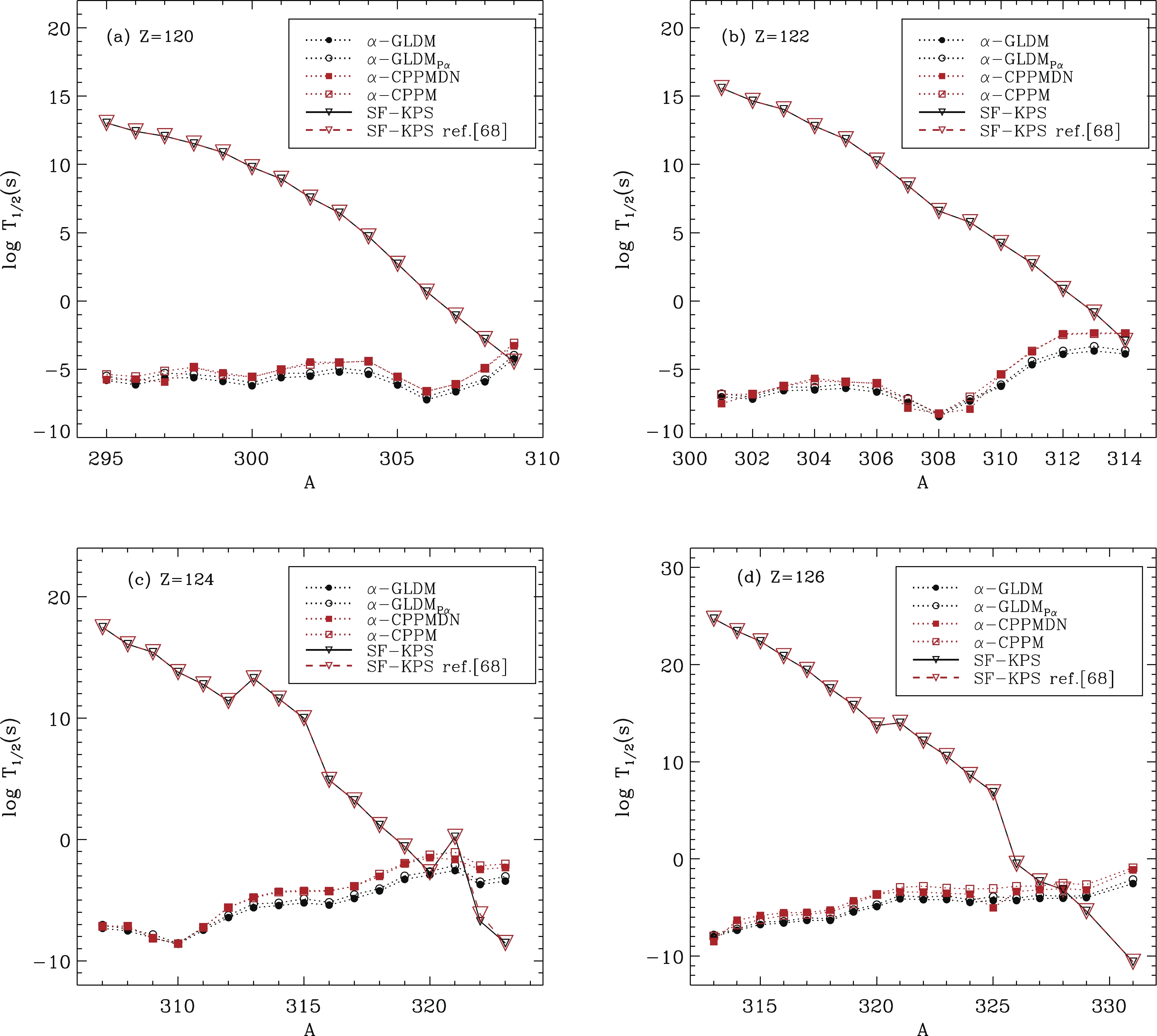
Figure 4. (color online) The
$ \alpha $ -decay half-lives and SF half-lives of$ ^{295-309} $ 120,$ ^{301-314} $ 122,$ ^{307-323} $ 124, and$ ^{313-331} $ 126. The$ \log_{10} $ $ T_{1/2}^{\alpha} $ values calculated with the Coulomb and proximity potential model (CPPM) and Coulomb and proximity potential model for deformed nuclei (CPPMDN) are from Ref. [79].As we use a fully phenomenological approach, we compare our results with those from calculations considering microscopic modifications [45]. As generally known, the
$ Q_{\alpha} $ values deduced would have an obvious influence on the calculated$ \alpha $ -decay half-lives. A 1 MeV change in the$ Q_{\alpha} $ value may lead to a change of around three orders of magnitude or more in the$ \log_{10} $ $ T_{1/2}^{\alpha} $ value. In Ref. [45], different mass tables are used to calculate$ Q_{\alpha} $ , including the WS4 mass table. Hence, we compare our$ \log_{10} $ $ T_{1/2}^{\alpha} $ with the$ \log_{10} $ $ T_{1/2}^{\alpha} $ value calculated with the WS4 mass model in Ref. [45]. In Fig. 3 from Ref. [45], the$ \log_{10} $ $ T_{1/2}^{\alpha} $ values of Z = 120,122,124 nuclei have dips at$ N_{d} $ = 184, where$ N_{d} $ represents the neutron number of the daughter nucleus. In this work, Fig. 2 shows the same trend for the$ \alpha $ -decay half-lives. The above discussion indicates that with similar$ Q_{\alpha} $ values, the results obtained with the phenomenological approach are highly consistent with the results from calculations considering microscopic modifications [81]. -
We used shell correction induced GLDM to calculate the
$ \alpha $ -decay half-lives of Z = 120, 122, 124, 126 isotopes. The preformation factor$ P_{\alpha} $ used in the model is of two types, where one is a constant for each type of nuclei, which was adopted from a least-squares fit to the known experimental half-lives (N$ \geqslant $ 152, Z$ \geqslant $ 82). The other type was calculated using the CFM. We compared our calculations with the experimental data for known nuclei from Fl to Og, and found that all the investigated methods could reproduce the$ \alpha $ -decay half-lives well. Subsequently, our method was used to predict the$ \alpha $ -decay properties of the even-Z SHN from Z = 120 to 126.The theoretical
$ P_{\alpha} $ values calculated using the CFM are very sensitive to the nuclear structure. The$ P_{\alpha} $ and$ Q_{\alpha} $ values show similar trends. They both reflect the position of shell structures. However,$ P_{\alpha} $ contains more complex shell structure information as it is adopted from several nearby nuclei. From the$ Q_{\alpha} $ and$ P_{\alpha} $ values, we present some nuclei that might be stable, i.e., Z = 120, N = 178, 184, 194, 196, 206, 218, 228; Z = 122, N = 182,184, 196, 202, 206, 216; and Z = 124, N = 204, 208, 216, 220. With larger proton numbers, more neutrons are needed for a nucleus to be stable.With the information of the
$ \alpha $ -decay half-lives, we find that at N = 184, there is no obvious shell structure for Z = 122, 124, 126 isotopes. The$ ^{304} $ 120 nucleus is predicted to be stable compared with the nearby nuclei. The competition between$ \alpha $ -decay and SF is increasing evident from Z = 120 to 126. However, the nuclei at around N = 184 would mostly undergo$ \alpha $ -decay. The predicted decay modes for$ ^{287-339} $ 120,$ ^{294-339} $ 122,$ ^{300-339} $ 124, and$ ^{306-339} $ 126 are presented in Table 2.We compared our results with other works, including the results obtained with microscopic calculations. The comparisons showed that the phenomenological and microscopic methods can produce highly similar
$ \alpha $ -decay half-lives, when similar$ Q_{\alpha} $ values are adopted. We suggest the selection of suitable$ Q_{\alpha} $ values, as the$ Q_{\alpha} $ values tend to clearly influence the calculations.The authors acknowledge the support provided by the Key Laboratory of Beam Technology of Ministry of Education, Beijing Normal University.
Calculations of the α-decay properties of Z = 120, 122, 124, 126 isotopes
- Received Date: 2009-04-30
- Available Online: 2020-10-01
Abstract: The


 DownLoad: