-
The existence of dark matter (DM) has been supported by substantial evidence from cosmology and astronomical observations [1]. A large number of direct searches for weakly interactive massive particles (WIMPs), a leading candidate of particle DM, are ongoing worldwide [2]. Over the last ten years, experiments employing dual-phase xenon time projection chambers (TPCs) have produced the most stringent constraints on the spin-independent interactions between WIMPs and nucleons, with a mass range from a few GeV/
$ {\rm c}^2 $ to 10 TeV/$ {\rm c}^2 $ [3-7].The PandaX-II experiment [8], conducted at the China Jinping Underground Laboratory (CJPL) [9], utilized a cylindrical dual-phase xenon TPC with a dodecagonal cross section (distance to opposite side: 646 mm) confined by polytetrafluoroethylene (PTFE) walls. The maximum drift distance is 600 mm in the vertical direction, defined by the distance from the bottom cathode mesh to the top gate grid. A total of 580 kg of liquid xenon is contained in the sensitive volume. Two arrays of Hamamatsu R11410-20 photomultiplier tubes (PMTs) located at the top and bottom of the TPC, respectively, view the sensitive volume. Recoil events produce the prompt scintillation photons (
$ S1 $ ) and delayed electroluminescence photons ($ S2 $ ). To achieve good collection of these photons, liquid xenon is purified with two circulation loops with a total mass flow rate of approximately 560 kg/d through hot getters to remove gaseous impurities. The relative sizes of$ S1 $ and$ S2 $ provide a powerful way to discriminate the electron recoil (ER) backgrounds from nuclear recoil (NR) signals.The analog waveform of each PMT, linearly amplified by a factor of approximately 10, is digitized by 100-MHz CAEN V1724 digitizers when an event is triggered either by
$ S1 $ or$ S2 $ . The digitizers used baseline suppression (BLS) firmware to suppress readouts for samples below the configurable threshold.Previous searches from PandaX-II have been reported in Refs. [3] (33 ton
$ \cdot $ day exposure) and [6] (54 ton$ \cdot $ day exposure). In this work, we report DM search results by combining all 132 ton$ \cdot $ day data obtained in PandaX-II with a blind analysis carried out on data in a fresh exposure. Major improvements in the data analysis are discussed in detail in this paper. The remainder of this paper is organized as follows. A simple description of the data sets is given in Sec. 2. The detailed data processing and improved event selections are discussed in Sec. 3. In Sec. 4, the data calibration, corrections, and signal models are presented. The backgrounds are analyzed in Sec. 5. The final candidates are reported in Sec. 6, from which we derive the exclusion limits in Sec. 7 using statistical analysis. -
The operation history and the accumulation of DM exposure in PandaX-II are summarized in Fig. 1. In total, three major DM runs have been coducted in PandaX-II: Run 9 [3], Run 10 [6], and Run 11. Immediately after 79.6 days of data collection in Run 9, an ER calibration with tritiated methane and a subsequent distillation campaign were performed, after which Run 10 collected DM search data for 77.1 days. Run 10 ended with a power failure, and Run 11 started right after the recovery, collecting a total of 244.2 days of data from July 17, 2017 to Aug. 16, 2018. The electron lifetime overlaid in Fig. 1 indicates the change of detector purity during the run. The first major drop in Run 11 ("A" in Fig. 1) was due to an unexpected power failure. The second drop, "B," occurred just after a neutron calibration, during which we varied the recirculation pump speed to study potential correlation with the background rate. The third drop, "C," occurred during a calibration run with
$ ^{220} {\rm{Rn}}$ injection [10], which introduced impurities into the detector. The last drop, "D," was caused by a real air leak into the detector due to a failed gate valve and, as a result, an increase in the ER background rate was observed. In the analysis presented, Run 11 is therefore broken down into two spans, span 1 and span 2, separated by "D," with live times of 96.3 and 147.9 days, respectively. After Run 11, the operation was dedicated to calibration and detector systematic studies before the official shutdown of PandaX-II on June 29, 2019. In Run 9, the cathode and gate electrodes were set at$ -29 $ kV and$ -4.95 $ kV, leading to an approximate drift field and electron extraction field of$ -400 $ V/cm and 4.56 kV/cm (in liquid xenon), respectively. In Runs 10 and 11, the cathode HV was lowered to$ -24 $ kV, leading to a different drift field of$ -317 $ V/cm.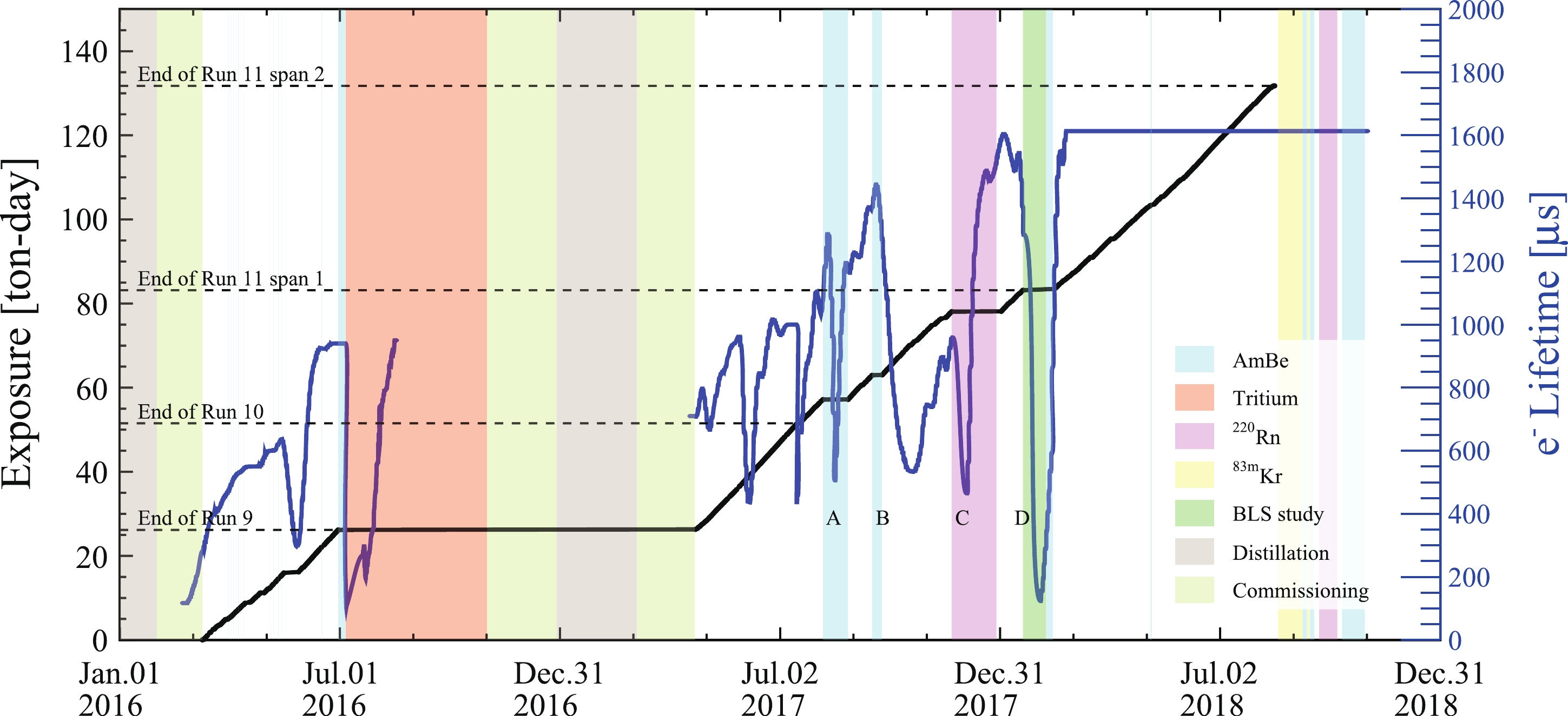
Figure 1. (color online) The accumulation of DM exposure (black line) and the evolution of the electron lifetime (blue curve, right axis) in PandaX-II. The black dashed horizontal lines indicate the divisions of data sets. Various colored bands represent the different operation modes, including NR calibration with AmBe source (cyan), ER calibration with tritium (pale red) and
$ ^{220} {\rm{Rn}}$ sources (pink),$ ^{83\rm{m}} {\rm{Kr}}$ calibration (yellow), baseline suppression study (green), xenon distillation (gray), and detector commissioning (light green).Calibration runs were interleaved with the DM data collection to study detector responses. One set corresponding to the 241Am-Be (AmBe) run was obtained at the end of Run 9. During and after Run 11, six more sets of AmBe runs were taken. They are used to characterize the NR responses. The low-energy ER responses are characterized with gaseous
$ \beta $ source injections runs, CH3T (tritium) or$ ^{220} {\rm{Rn}}$ , for Run 9 and Runs 10/11, respectively. Other types of calibration runs include a$ ^{83\rm{m}} {\rm{Kr}}$ injection run for position reconstruction studies and uniformity correction (Run 11), and external$ ^{137} {\rm{Cs}}$ and$ ^{60} {\rm{Co}}$ source deployment to calibrate detector response to higher energy gammas. -
The basic data processing procedure from previous analyses [8, 11] was followed in this analysis. Only major improvements are highlighted here, including a) inhibiting unstable PMTs for better consistency among data sets, b) an improved gain calibration for low gain PMTs, c) refinements of data quality cuts, and d) substantial improvements in the position reconstruction algorithm. For the DM search in Run 11, we blinded the data with
$ S1 $ less than 45 PE (previous search window) to avoid subjective choices until the background estimation was finalized. -
For consistency, particularly in terms of position reconstructions, seven malfunctioning PMTs (five top, two bottom) among the 110 R11410-20 PMTs are fully inhibited in this analysis for all data sets. Among them, three were turned off in Ref. [6], one due to severe afterpulsing, and two due to failures in PMT bases. During Run 11, four more PMTs became unstable; one was physically turned off due to the high discharge rate, and the other three were inhibited by software: one due to afterpulsing, and the other two due to abnormal gains and baseline noises. The five inhibited top PMTs are indicated in Fig. B1 in Appendix B.
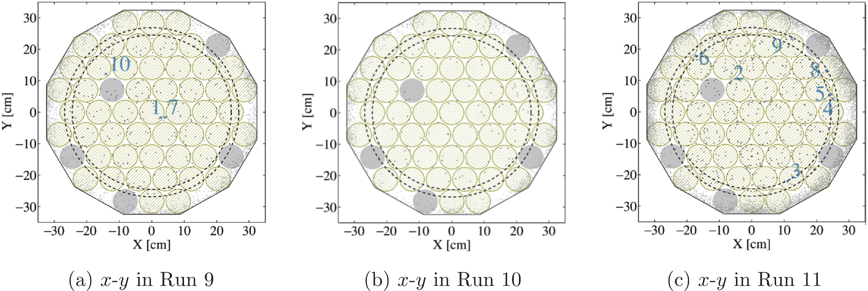
Figure B1. (color online) x vs. y distribution of the events in the
$ S2 $ and$ S1 $ range cut of DM search runs. The drifting time cut,$ (18,310) $ μs in Run 9 (a) and$ (50,350) $ μs in Run 10 (b) and 11 (c) is applied to all events. The top ten DM-like candidates are labeled. The dashed lines mark the$ R^{2} = 720 $ cm$ ^{2} $ and$ R^2 = 600 $ cm$ ^{2} $ . The dodecagon is the boundary of the detector. The yellow (gray) circles represent the normal (inhibited) PMTs of the top array. -
PMT gains were calibrated twice a week using low-intensity blue light-emitting diodes (LEDs) inside the detector by fitting the single photoelectron (SPE) peak in the spectrum. After a vacuum failure between Runs 9 and 10, which may have caused degradation in some high-voltage feedthroughs, a number of PMTs could only run at lower high voltages. Some had to be gradually lowered throughout Runs 10 and 11. These led to significantly reduced gain values (average gain changed from 1.41
$ \times10^{6} $ in Run 9 to 0.96$ \times10^{6} $ in Run 11, before the linear amplifiers). For low gain channels ($ \sim10^5 $ ), the LED calibration had two problems. First, the corresponding SPE peaks could not be distinguished from baseline noises, leading to failed fits and jumps. Second, the LED calibration could not catch up with the temporal change of the gains.To mitigate these effects, we developed in situ gain estimates by selecting alpha events and using the mean
$ S1 $ charge in the normal PMTs located at the same radius in the same array as a reference. This procedure is illustrated in Fig. 2. After this correction, the gain evolution of all channels becomes stable.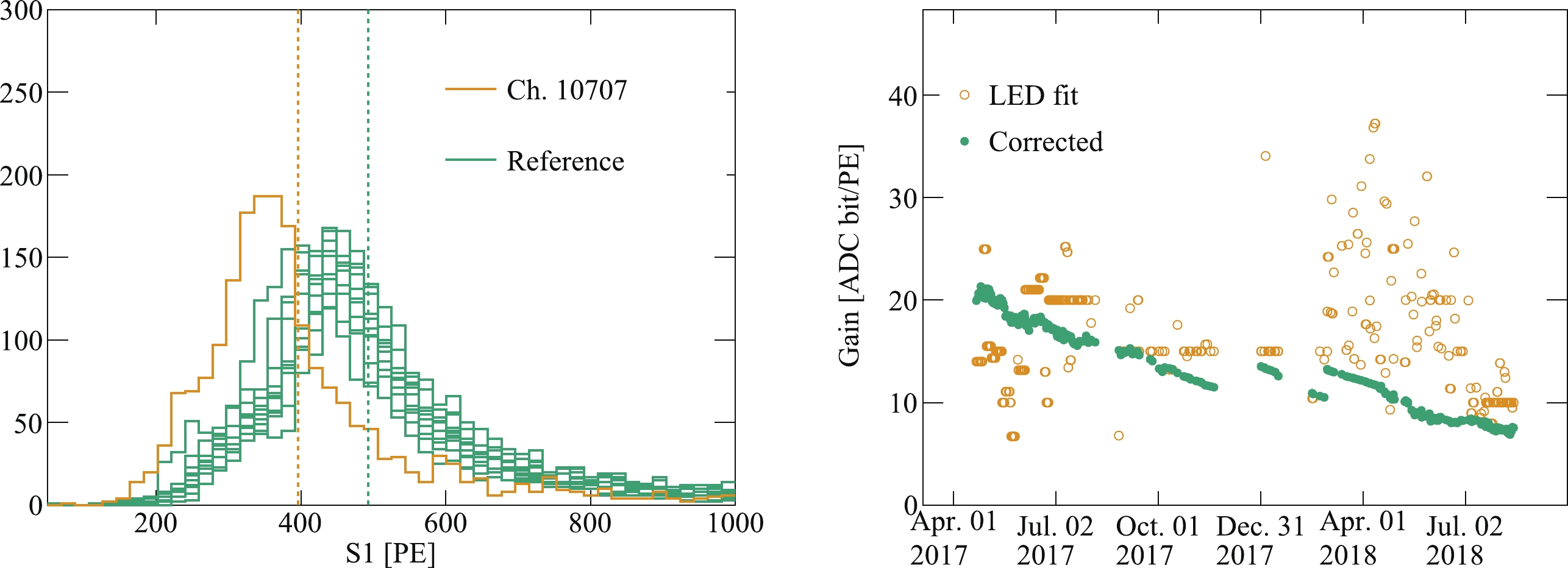
Figure 2. (color online) An example of gain correction to low gain PMTs. (left) The
$ S1 $ charge distribution of$ \alpha $ events in the low gain Ch.10707 (yellow line) and the other reference PMTs located at the same radius (green lines). The yellow and green dashed lines mark the mean of the$ S1 $ detected by Ch.10707 and the reference PMTs, respectively. The ratio of the means is used to correct the gain of Ch.10707. (right) The evolution of gain of Ch.10707. The yellow open circles represent gains obtained in the LED calibration and the green dots are the corrected gains. The gradual decrease is due to the continuous reduction of the supply voltage, and the residual jumps are due to the attempts to recover the high voltage during the run. -
The data selection cuts used in Ref. [8] are also inherited in this analysis. The criteria for some cuts have been updated in this analysis due to the updated PMT configurations. Two more cuts are developed to suppress spurious events. 1) In PandaX-II, the PMT cathode and metal housing were set at approximately
$ -700 $ V. Ionized electrons produced in the gaseous region between the top PMT array and the anode (ground) would drift toward the anode and some may get amplified close to the anode wires, producing$ S2 $ s. These events have a typical drift time of$ \sim $ 40 μs, and due to longer tracks and diffusions in weak drift fields, these$ S2 $ s have larger width in comparison with the normal events. A cut on the$ S2 $ widths is developed and applied. 2) We observed that occasionally some mini-discharges occurred in the detector, resulting in waveforms containing “trains” of small pulses. A cut on the “cleanliness” of the waveform is developed to remove such events. By analzing the NR and ER calibration data, the inefficiency of the two cuts for “good” single-scattering events is estimated to be less than 5%.The loss of efficiency is more significant for smaller signals, and it gradually plateaued. Similar to the previous analyses, the overall selection efficiency can be parameterized into
$ \epsilon = \epsilon_1(S1)\epsilon_2(S2)\epsilon_{\rm{BDT}}\epsilon_{\rm{plateau}}\,, $

(1) in which
$ \epsilon_1(S1) $ ($ \epsilon_2(S2) $ ) are$ S1 $ ($ S2 $ ) data quality cut efficiency normalized to unity toward high energy, which is discussed in Sec. 4.4, and$ \epsilon_{\rm{BDT}} $ refers to the efficiency of the boosted decision tree (BDT) cut to suppress accidental backgrounds (see Sec. 5). The plateau efficiency from all quality cuts is estimated to be 91% for$ S1 > 20 $ PE and$ S2_{\rm{raw}} $ (uncorrected for uniformity)$ >500 $ PE, by studying the NR events in AmBe calibration runs within the$ \pm3\sigma $ region of the NR band. -
Only single scattered events, containing a single
$ S1 $ and$ S2 $ pair, are selected for final analysis. The separation between the two signals determines the vertical position of the event, by assuming a constant drift velocity. The maximum drift time is measured to be 350 μs in Run 9 and 360 μs in Runs 10 and 11 due to differences in drift fields.The horizontal position is extracted from the
$ S2 $ charge pattern on the top PMT array, exploiting a data-driven photon acceptance function (PAF), i.e., the proportion of$ S2 $ deposited onto each PMT for a given horizontal position. In Ref. [3], the PAF was parameterized analytically, which allowed position reconstruction via a likelihood fit. However, it is found that reconstructed positions have local distortions (clustering toward the center of the PMTs). It is also not sufficiently stable with PMTs turned off. In this analysis, we develop an improved PAF method utilizing the$ ^{83\rm{m}} {\rm{Kr}}$ calibration data obtained in 2018, with ER peaks of 41.6 keV distributed throughout the detector. The procedure is as follows.1. The average charge pattern of
$ S2 $ on the top PMT array is extracted for each given reconstructed position pixel, using the analytical PAF as the starting point.2. Geant4 [12, 13] optical simulations with realistic PandaX-II geometry and optical properties are carried out, assuming
$ S2 $ photons are produced as a point photon source in the gas gap. The vertical photon production point$ z_{S2} $ is adjusted for each horizontal position to find a match in charge pattern between the data and the simulations.3. Once the optimal
$ z_{S2}(x,y) $ is found, a new PAF is produced, based entirely on the tuned Geant4 simulations. The$ ^{83\rm{m}} {\rm{Kr}}$ positions are reconstructed again using the new PAF, after which a new data-driven charge pattern vs. position is produced.This procedure is carried out iteratively until the reconstruction becomes stable. It outperforms the previous method significantly, especially after the malfunctioned PMTs are inhibited, as shown in Fig. 3. For each event, the difference between the horizontal positions reconstructed by the new and old method is required to be smaller than 40 mm, serving as a data quality cut. The uncertainty in horizontal position is estimated to be 5 mm based on the
$ ^{83\rm{m}} {\rm{Kr}}$ data, which propagated into an uncertainty in the fiducial volume (FV). -
Various calibration runs were performed throughout the PandaX-II operation to measure detector responses, such as the signal uniformity, the single electron gain (SEG), the average photon detection efficiency (PDE), and the electron extraction efficiency (EEE), and to model the low-energy DM signal and background events. We discuss them in turn.
-
Mono-energetic events uniformly distributed in liquid xenon are selected to calibrate the non-uniform distribution of detected signals. The correction to
$ S1 $ is a smooth three-dimensional map based on the internal background peaks, since there is no simple analytical parameterization. The correction of$ S2 $ s is separated into two parts, first an exponential attenuation in the vertical direction due to electron losses during the drift, parameterized by the electron lifetime (see Fig. 1), then a two-dimensional smooth map based on internal background peaks. Ideally, in situ background peaks keep track with potential temporal changes in the detector; thus, they are the best choice for uniformity correction, but statistics are also an important consideration. In the three runs, the corrections are obtained differently, as summarized in Table 1.Item Run 9 Run 10 Run 11 $ S1 $ 

$ ^{131\rm{m}} {\rm{Xe}}$ 

$ ^{83\rm{m}} {\rm{Kr}}$ 

$ ^{83\rm{m}} {\rm{Kr}}$ 

$ S2 $ electron lifetime

$ ^{131\rm{m}} {\rm{Xe}}$ 

$ ^{131\rm{m}} {\rm{Xe}}$ 

internal $ \alpha $ 

$ S2 $ horizontal

$ ^{131\rm{m}} {\rm{Xe}}$ and tritium

$ ^{131\rm{m}} {\rm{Xe}}$ 

$ ^{83\rm{m}} {\rm{Kr}}$ 

Table 1. Uniformity calibration approach used in the three runs.
In Run 9, due to the long exposure of xenon on the surface, the detector has a rather high rate of 164-keV gamma events from the neutron-activated
$ ^{131\rm{m}} {\rm{Xe}}$ , based on which both$ S1 $ and$ S2 $ maps are produced. In Run 10, the$ S2 $ horizontal correction and the electron lifetime are obtained from$ ^{131\rm{m}} {\rm{Xe}}$ , but the three-dimensional$ S1 $ correction is based on the$ ^{83\rm{m}} {\rm{Kr}}$ data in 2019 due to its excellent statistics. In Run 11, as the$ ^{131\rm{m}} {\rm{Xe}}$ rate becomes insufficient, a$ ^{83\rm{m}} {\rm{Kr}}$ map is applied to the$ S1 $ and$ S2 $ horizontal corrections. The electron lifetime, on the other hand, is obtained in situ using$ ^{222} {\rm{Rn}}$ and$ ^{218} {\rm{Po}}$ alpha events with$ S2_b $ , the portion of$ S2 $ detected by the bottom PMT array. On the other hand, in Ref. [14], the electron lifetime was obtained based on the high energy gamma data to optimize the resolution in that regime, but may already contain the saturation effects. The$ ^{83\rm{m}} {\rm{Kr}}$ maps used in Run 11 for$ S1 $ (two projections) and$ S2 $ are shown in Fig. 4. The maximum variations in the FV are [-19.0%, 30.2%] in$ S1 $ and [-31.9%, 16.4%] in$ S2 $ .
Figure 4. (color online) The non-uniformity correction map obtained from the
$ ^{83\rm{m}} {\rm{Kr}}$ data for$ S1 $ and$ S2 $ .Note that
$ S2 $ photons are substantially clustered on the top PMT array; therefore, they are subject to saturation effects. In this analysis, both$ S2 $ and$ S2_b $ are corrected using their corresponding maps according to Table 1. It is found that that the$ S2 $ map in Run 9 (when most PMTs were operated under normal gain) is biased due to saturation; thus, the$ S2 $ horizontal map is further corrected based on the mean value of the$ S2 $ s in the tritium calibration data. -
The BLS threshold for each digitizer channel was set at an amplitude of 2.75 mV above the baseline. For comparison, the SPE for a gain of 106 corresponds to a mean amplitude of 4.4 mV in the digitizer. Although the gains vary from PMT to PMT, fixed thresholds are needed to avoid excessive data size due to baseline noises. The channel-wise BLS inefficiency is negligible for Run 9, since all PMTs were operating under the normal gain, but it becomes more significant during Runs 10 and 11 due to the low-gain PMTs (Sec. 3.2). Consequently, the detected
$ S1_d $ and$ S2_d $ are suppressed from the actual$ S1 $ and$ S2 $ . As long as$ S1_d $ and$ S2_d $ fall into selection windows, BLS does not cause an event loss but rather a nonlinearity in$ S1 $ and$ S2 $ , stronger for small signals and approaching unity for large ones.The nonlinearities depend subtly on the shapes and actual distributions of
$ S1 $ and$ S2 $ on individual PMTs. Therefore, instead of adopting the single-channel BLS efficiency from the LED calibration, as in Ref. [6], in Run 11 we performed direct measurement using neutron calibration data with low-energy events distributed throughout the detector. During this special data acquisition, the BLS firmware was disabled, so that all waveform data were saved (thresholdless), and the standard$ S1 $ and$ S2 $ identifications were performed on the data①. We then applied the BLS algorithm on the data as that in the firmware and obtained$ S1_d $ and$ S2_d $ , from which the BLS nonlinearities$ f_1 = \dfrac{S1_d}{S1} $ and$ f_2 = \dfrac{S2_d}{S2} $ were determined in an event-by-event manner. The distributions of$ f_1 $ and$ f_2 $ are shown in Fig. 5 with clear spreads due to fluctuations in the data. They are modeled into smooth probability density functions (PDFs) when later converting$ S1 $ and$ S2 $ into$ S1_d $ and$ S2_d $ in our signal and background models. In the remainder of this paper,$ S1 $ and$ S2 $ refer to the detected$ S1_d $ and$ S2_d $ for simplicity, unless otherwise specified. -
With updates in the lower-level analysis mentioned above, we extract detector parameters for Runs 9 and 10. For each event, the energy is reconstructed as
$ E_{\rm{rec}} = 0.0137\,{\rm{keV}}\times \left(\frac{S1}{\rm{PDE}}+\frac{S2}{{\rm{EEE}}\times{\rm{SEG}}}\right), $

(2) where
$ S1 $ and$ S2 $ have been corrected for uniformity in all the runs and BLS nonlinearity in Runs 10 and 11. Note that in all three run sets,$ S2 $ saturation is found for energy higher than 200 keV. For conservativeness, for energy higher than 30 keV, we calculate$ S2 $ as$ \alpha \times S2_b $ , and$ \alpha $ is 3.0 and 3.18 for Run 9 and Runs 10/11, determined using data in the low-energy DM search region. The SEG is determined by selecting the smallest$ S2 $ s, and the spectrum is fitted with a combination of a threshold function and a double Gaussian encoding the single and double electron signals. The best fit parameters of PDE and EEE are determined by performing a parameter scan when fitting the energy spectra of known ER peaks from the calibration data, requiring a global minimization of$ \chi^2 $ between the reconstructed and expected energies.In Run 9, we select the prompt de-excitation gamma rays from the neutron calibration, 39.6 keV from
$ ^{129} {\rm{Xe}}$ , and 80.2 keV from$ ^{131} {\rm{Xe}}$ , both corrected for the small shifts caused by the mixture of NR energy. ER peaks due to the same neutron illumination, 164 keV ($ ^{131\rm{m}} {\rm{Xe}}$ ) and 236 keV ($ ^{129\rm{m}} {\rm{Xe}}$ ), are also selected. For higher energy gamma peaks, we only select the 662 keV peak from$ ^{137} {\rm{Cs}}$ to avoid potential bias in energy due to the saturation of$ S2 $ . In Run 10, to avoid BLS nonlinearities at lower energies, higher energy peaks, including 164, 236, 662 keV, together with gammas of 1173 and 1332 keV from$ ^{60} {\rm{Co}}$ , are selected. The systematic uncertainty of each peak is initially set to be 1%, guided by the sensitivity of the 164 keV to data cuts, uniformity corrections, fit range, temporal drifts, etc. Additional uncertainties are assigned to peaks that entail more uncertainty due to saturation effects, mixture of NR, etc. The quality of the fits is illustrated in Fig. 6 where the relative differences between the reconstructed and the expected energies are plotted. Peaks not used in fitting serve as critical checks, shown as the open symbols in the figure. The overall agreement is better than 3%. The uncertainties of PDE and EEE are estimated based on parameter contours bounded by$ \Delta\chi^2 = 1 $ .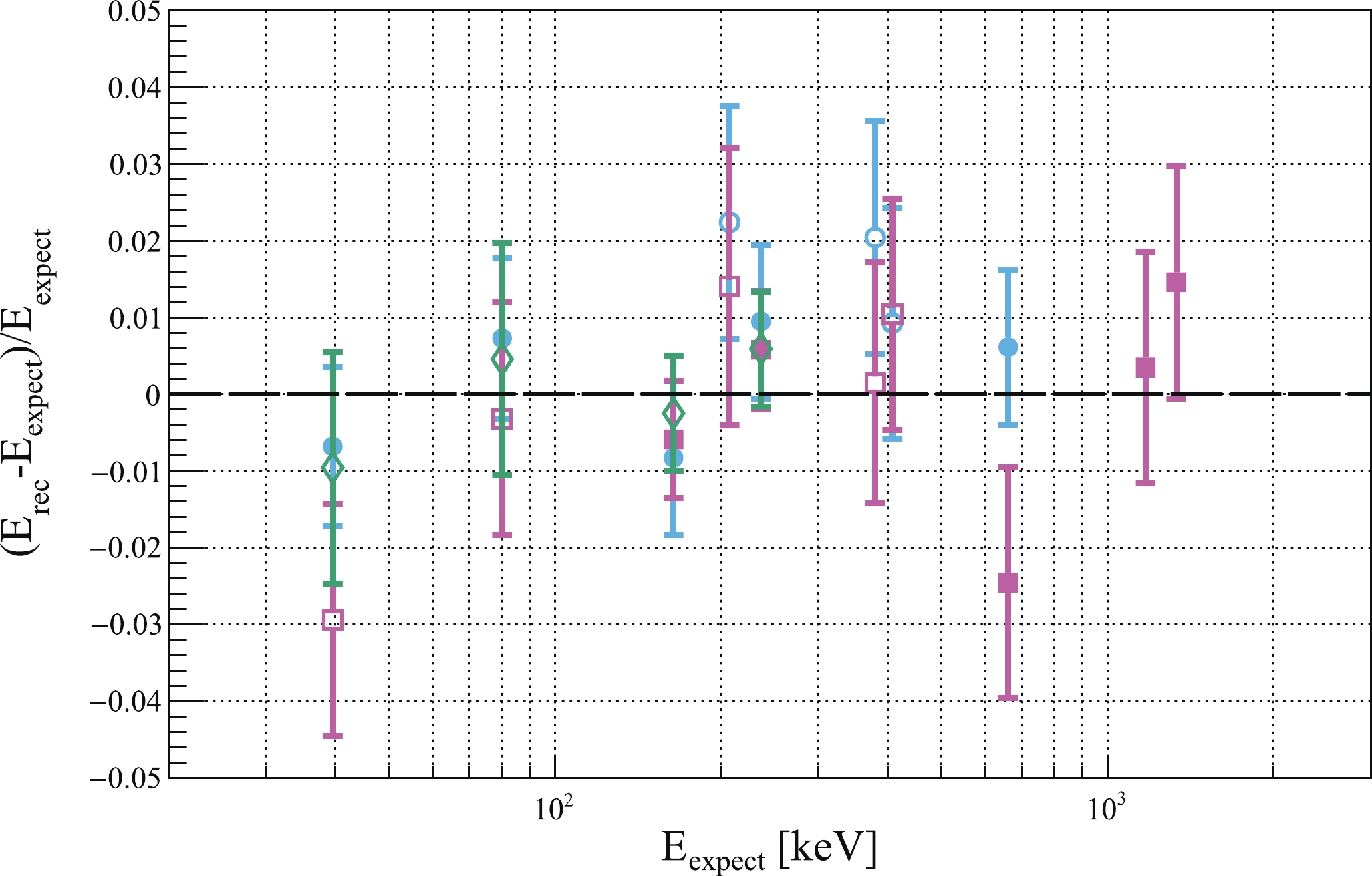
Figure 6. (color online) Fractional difference between the reconstructed energy
$ E_{\rm{rec}} $ and expected energy$ E_{\rm expect} $ for characteristic gamma peaks in Run 9 (blue circles), Run 10 (magenta squares), and Run 11 (green diamonds). Peaks include 39.6 keV (n,$ ^{129} {\rm{Xe}}$ ), 80.2 keV (n,$ ^{131} {\rm{Xe}}$ ), 164 keV ($ ^{131\rm{m}} {\rm{Xe}}$ ), 236 keV ($ ^{129\rm{m}} {\rm{Xe}}$ ), 202.8,375, and 408 keV ($ ^{127} {\rm{Xe}}$ ), 662 keV ($ ^{137} {\rm{Cs}}$ ) and 1173 and 1332 keV($ ^{60} {\rm{Co}}$ ). Uncertainties are dominated by systematic components. Closed symbols represent points used in the fits, and open symbols are those test peaks. See text for details.The resulting parameters in different run sets are summarized in Table 2. For Run 11, since the field configurations stays the same as in Run 10, the PDE and EEE are obtained by scaling the Run 10 values according to the average
$ S1 $ and$ S2 $ from the 164-keV peak in the detector.Run PDE (%) EEE (%) SEG (PE/ $ e^- $ )

9 $ 11.5\pm0.2 $ 

$ 46.3\pm1.4 $ 

$ 24.4\pm0.4 $ 

10 $ 12.1\pm0.5 $ 

$ 50.8\pm2.1 $ 

$ 23.7\pm0.8 $ 

11 $ 12.0\pm0.5 $ 

$ 47.5\pm2.0 $ 

$ 23.5\pm0.8 $ 

Table 2. Summary of PDE, EEE, and SEG in three DM search data runs in PandaX-II.
-
For the ER calibration, as in Ref. [6], the tritiated methane data are used for Run 9, but reanalyzed using an updated PMT configuration and uniformity correction. Different from Ref. [6], the two
$ ^{220} {\rm{Rn}}$ data sets in Run 11 [14] are combined and used for both Runs 10/11. For the NR calibration, in Run 11, 19,158 low energy single-scatter NR events in the FV are identified, allowing a more accurate modeling of the NR responses. These data are used as the NR calibration for both Run 10 and Run 11.The distributions of
$ \log_{10}(S2/S1) $ vs.$ S1 $ for ER and NR calibration events in Run 9 and Runs 10/11 are shown separately in Fig. 7. As expected, a shift in the ER distribution is observed due to different drift fields, but not in the NR distribution [15]. The discrimination power of the detector to reject ER backgrounds can be evaluated by the leakage ratio r, defined as the number of ER signals leaking below the NR band median, which is measured in Fig. 7 to be$ 53/7089 = 0.75\pm0.10 $ % in Run 9, and$ 28/3463 = 0.81\pm0.15 $ % in Runs 10/11.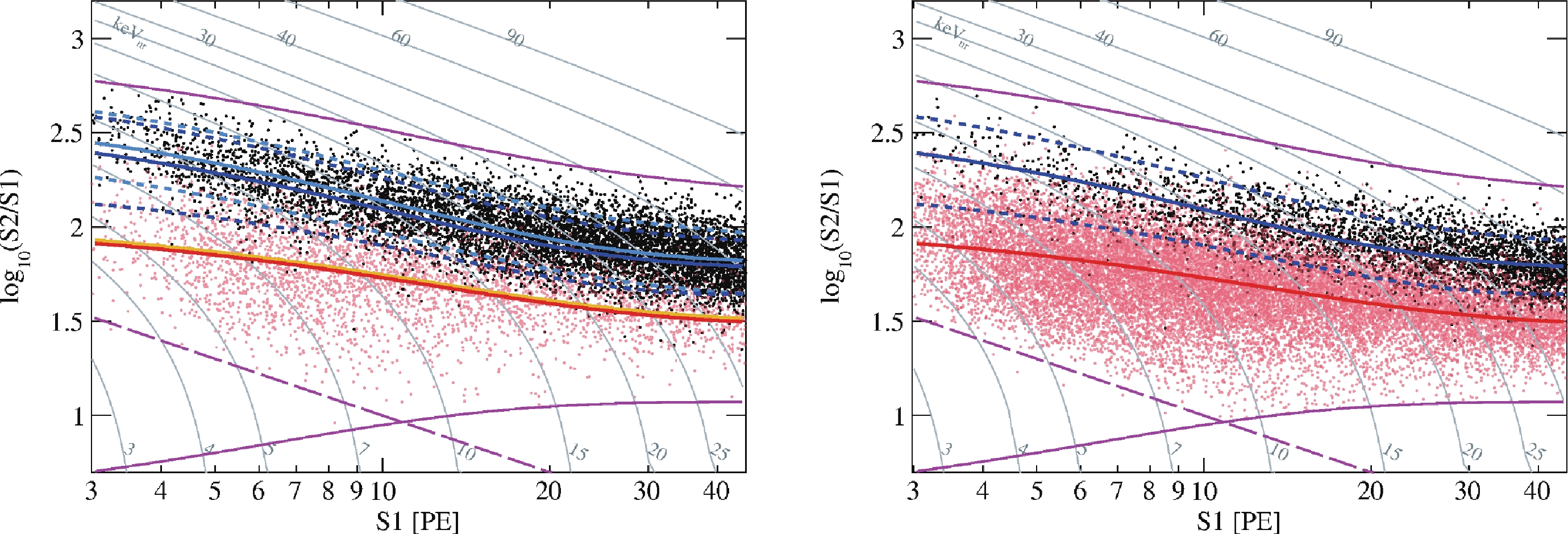
Figure 7. (color online) The distributions of calibration data in Run 9 and Runs 10/11 in
$ \log_{10}(S2/S1) $ vs.$ S1 $ : ER (black), NR (red). The light and dark blue lines represent the fitted ER medians for Run 9 and Runs 10/11, respectively, and the dashed blue lines are the corresponding 90% quantiles. The orange and red lines represent the fitted NR medians for Run 9 and Runs 10/11, respectively. The impact of differences in PDE/EEE/SEG is confirmed to be negligible.Our ER and NR response model follows the construction of the so-called NEST2.0 [16]. In this analysis, the initial excitation-to-ionization ratio,
$ N_{\rm{ex}}/N_{\rm i} $ , is taken from NEST2.0. On the other hand, the charge yield and light yield (per unit energy) are initially fitted from the centroids of our data as$ \mathrm{CY}_0 = \frac{S2}{\mathrm{EEE}\times \mathrm{SEG}}/E_{\mathrm{rec}}\,,\;\;\;\; \mathrm{LY}_0 = \frac{S1}{\mathrm{PDE}}/E_{\mathrm{rec}}\,, $

(3) where the so-called electron-equivalent energy is reconstructed based on Eq. (2). For an NR event, the NR energy is estimated by further dividing out the so-called Lindhard factor [17]. Note that
$ E_{\rm{rec}} $ contains energy smearing introduced by the fluctuations in$ S1 $ and$ S2 $ . Therefore NEST2.0-based simulations are carried out in which CY and LY are adjusted iteratively until a good fit in the two-dimensional distributions in the data and simulation is reached. Our model also takes into account the detector parameters extracted above and the spatial non-uniformity (Sec. 4.1), the double photoelectron emission measured in situ ($ \sim $ 21.5%) [6], and the SPE resolution to properly include the fluctuations. In the simulation,$ S1 $ is randomly distributed onto individual PMTs so that the three-PMT coincidence selection cut could be simulated. The BLS nonlinearity is included in$ S1 $ and$ S2 $ . To fit the entire data distribution, the fluctuation in the recombination rate is tuned against the calibration as well. The comparisons between our best model simulation and calibration data in$ S1 $ ,$ S2 $ , and$ E_{\rm{rec}} $ are shown in Fig. 8, in which good agreement is found.
Figure 8. (color online) The comparison of model simulation and calibration data in the projection of deposited energy,
$ S1 $ and$ S2 $ , in Run 9 and Runs 10/11.We also compare the aforementioned ER model with the ER event distributions in Runs 10 and 11 by selecting the events within
$ S1\in(45,200) $ PE (outside DM search window; see Sec. 6). Although the band centroids agree well, the observed width in the data is larger than that from the calibration (Fig. 9), presumably due to the accumulated fluctuations over time. Therefore, we increase the fluctuations in the ER model for Runs 10 and 11 accordingly, leading to larger leakage ratios r (see Table 5 in Sec. 5).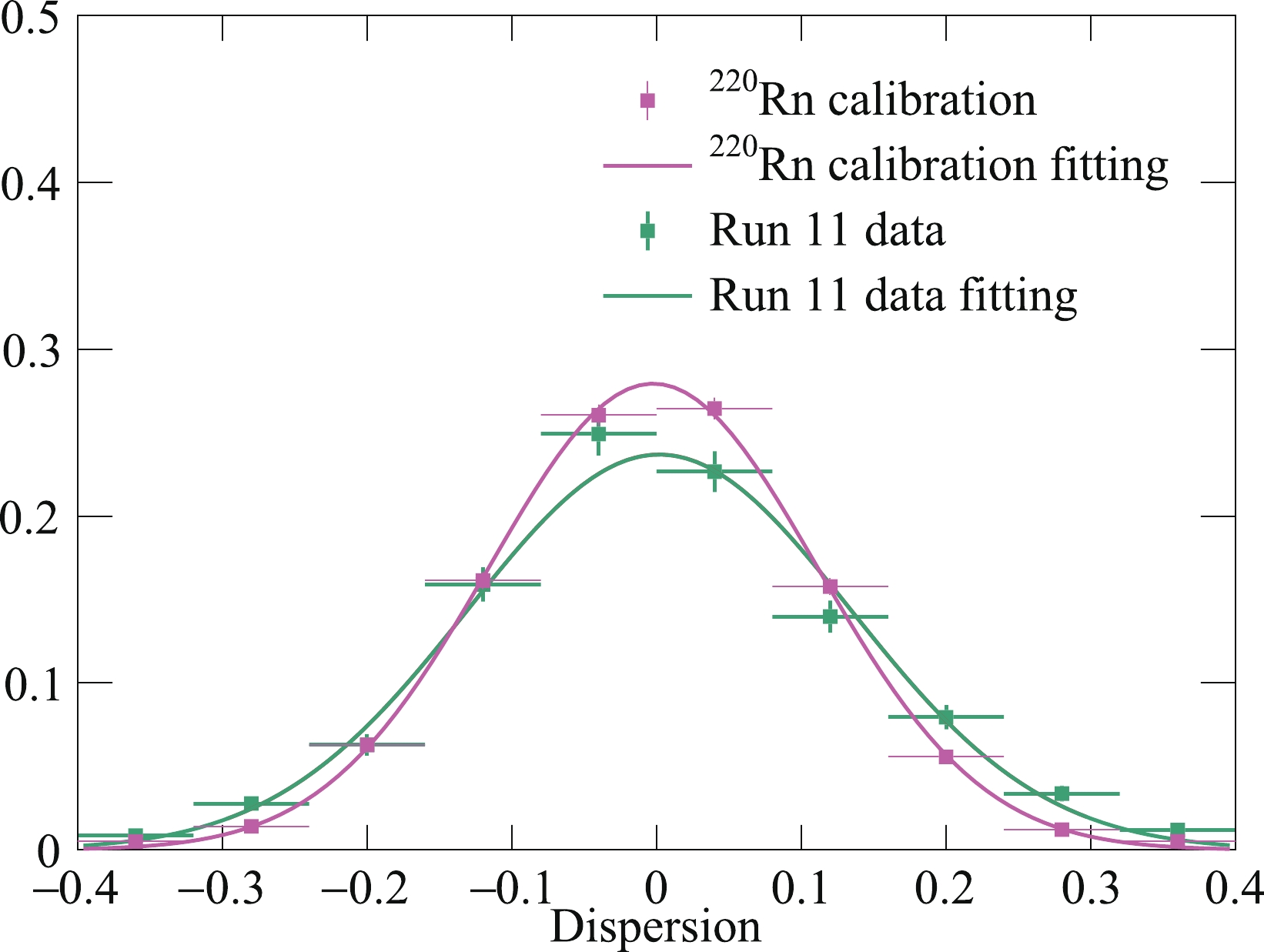
Figure 9. (color online) Comparison of the distribution of events away from the median of ER band with
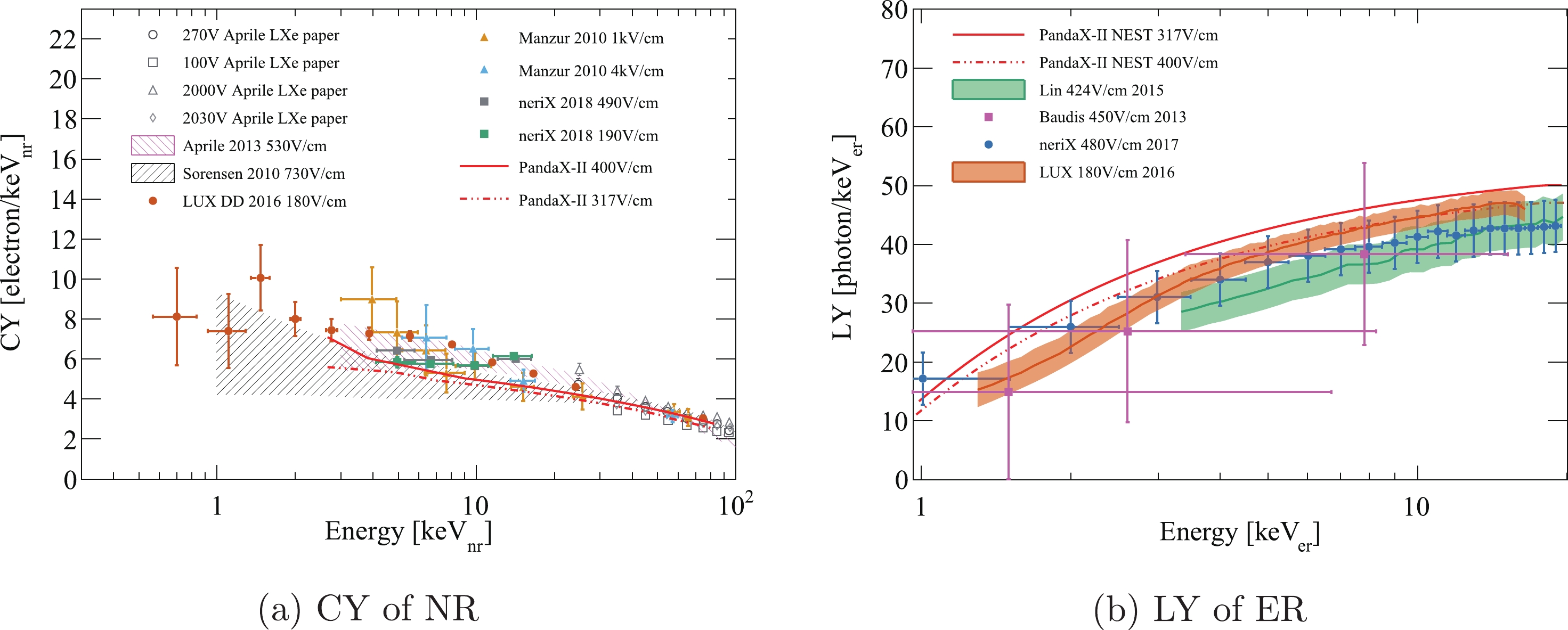
$ S1\in (45,200) $ PE between the$ ^{220} {\rm{Rn}}$ calibration data (magenta dots) and Run 11 DM search data (green dots). The fitted Gaussian functions are overlaid.The best fit LY (for ER) and CY (for NR) in PandaX-II are plotted in Fig. 10, together with the values from other xenon-based experiments. Our NR model is in agreement with the worldwide data within uncertainties. On the other hand, our ER model is consistent with that of Ref. [18], but has certain dissimilarities with those of Refs. [19-21]. Nevertheless, since our model describes the calibration data, it is a self-consistent model for producing the signal and background distributions.
The
$ S1 $ and$ S2 $ simulations noted above do not include the data quality cut efficiencies. Therefore, anchoring the distributions at the high end,$ \epsilon_1 $ and$ \epsilon_2 $ , in Eq. (1) can be performed by a comparison between the simulation and data. This is also illustrated in Fig. 8. Because$ \epsilon_1 $ agrees well for NR and ER events, we adopted$\epsilon_1 = 1/ \bigg({1\!+ \exp\left(\dfrac{S1\!-\!3.1}{0.075}\right)}\bigg)$ (Run 9) and$ \epsilon_1 \!=\! 1/\left({1\!+\!\exp\left(\dfrac{S1\!-\!4.0}{0.8}\right)}\right) $ (Runs 10/11). It is found that no$ S2 $ efficiency is needed, presumably due to the fact that our analysis cut is for$ S2_{\rm raw}>100 $ PE, but the$ S2 $ trigger threshold is approximately 50 PE [27]. -
After all data selections, four main backgrounds remain in the data: the ER, neutron, accidental, and surface background. Improvements of the estimates are addressed in turn.
The ER backgrounds come from varies sources, including gammas from radioactive decay in the detector materials, the radioactive xenon isotope of
$ ^{127} {\rm{Xe}}$ (Runs 9 and 10), the beta decay of tritium (Runs 10 and 11), radioactive krypton and radon identified in the detector, the solar neutrinos, and the double beta decay of$ ^{136} {\rm{Xe}}$ . A summary of the background level is presented in Table 3.Item Run 9 Run 10 Run 11, span 1 Run 11, span 2 flat ER (mDRU) $ ^{85} {\rm{Kr}}$ 

$ 1.19\pm0.2 $ 

$ 0.18\pm0.05 $ 

$ 0.20\pm0.06 $ 

$ 0.40\pm0.07 $ 

$ ^{222} {\rm{Rn}}$ 

$ 0.19\pm0.10 $ 

$ 0.17\pm0.02 $ 

$ 0.19\pm0.02 $ 

$ 0.19\pm0.02 $ 

$ ^{220} {\rm{Rn}}$ 

$ 0.01\pm0.01 $ 

$ 0.01\pm0.01 $ 

$ 0.01\pm0.01 $ 

$ 0.01\pm0.01 $ 

ER (material) $ 0.20\pm0.10 $ 

$ 0.20\pm0.10 $ 

$ 0.20\pm0.10 $ 

$ 0.20\pm0.10 $ 

solar $ \nu $ 

$ 0.01 $ 

$ 0.01 $ 

$ 0.01 $ 

$ 0.01 $ 

$ ^{136} {\rm{Xe}}$ 

$ 0.0022 $ 

$ 0.0022 $ 

$ 0.0022 $ 

$ 0.0022 $ 

total flat ER (mDRU) $ 1.61\pm0.24 $ 

$ 0.57\pm0.11 $ 

$ 0.73\pm 0.08 $ 

$ 1.03\pm0.08 $ 

$ ^{127} {\rm{Xe}}$ (mDRU)

$ 0.14\pm0.03 $ 

$ 0.0069\pm0.0017 $ 

<0.0001 3H (mDRU) 0 $0.11$ 

neutron (mDRU) $ 0.0022\pm 0.0011 $ 

accidental (event/day) $ 0.014\pm 0.004 $ 

surface (event/day) $ 0.041\pm0.008 $ 

$ 0.063\pm 0.0013 $ 

Table 3. Backgrounds in the dark matter search runs inside the FV. Among the ER backgrounds, the radioactivity level of 3H is from the best fit. Others are estimated independently. ER and neutron backgrounds are estimated in
$ 0 $ -$ 25 $ keV. Accidental and surface backgrounds are estimated in the search window of S1 within$ 3 $ -$ 45 $ PE and S2 within$ 100 $ (raw)-$ 10000 $ PE.$ 1 $ mDRU =$ 1\times10^{-3} $ evt/keV/d/kg. The total flat ER backgrounds of Runs 9 and 10 are sums of the components, and that of Run 11 is estimated with data in the region of 20-25 keV (see text for details).The estimates of the ER backgrounds from the detector material, solar neutrinos, and
$ ^{136} {\rm{Xe}}$ used in a previous analysis [8] are inherited.The
$ ^{127} {\rm{Xe}}$ background is also inherited from Ref. [6]. Due to the relatively short half-life (35.5 d), no$ ^{127} {\rm{Xe}}$ events are identified in Run 11.A significant tritium background is introduced in the CH
$ _{3} $ T calibration in 2016 after Run 9, and it could not be effectively removed by hot getters. The distillation campaign thereafter reduced the tritium level by a factor of roughly 100. The residual tritium rate is found to be stable at$ 0.030 \pm 0.004 $ μBq/kg, based on unconstrained fits to data in different runs within (0, 10] keV.The level of the
$ ^{220} {\rm{Rn}}$ background is estimated by the$ ^{212} $ Bi-$ ^{212} {\rm{Po}}$ and$ ^{220} {\rm{Rn}}$ -$ ^{216} {\rm{Po}}$ coincidence events. The updated$ ^{220} {\rm{Rn}}$ level is$ 0.37\pm0.20 $ μBq/kg in Runs 10 and 11. For$ ^{222} {\rm{Rn}}$ , the dominating background in the DM region is the$ \beta $ -decay of the daughter$ ^{214} {\rm{Pb}}$ . In Ref. [14], it is found that ions from the$ ^{222} {\rm{Rn}}$ decay chains would drift toward the cathode, causing a decay rate depletion for decay daughters in the FV. Based on this study, a more robust method for estimating the$ ^{214} {\rm{Pb}}$ background is developed by combining the$ \alpha $ rate from$ ^{222} {\rm{Rn}}$ and$ ^{218} {\rm{Po}}$ and$ \beta $ -$ \alpha $ coincidence of$ ^{214} $ Bi-$ ^{214} {\rm{Po}}$ [14]. The resulting$ ^{214} {\rm{Pb}}$ level is found to be rather stable in the three data sets, at approximately 10 μBq/kg.Krypton causes one of the most critical backgrounds in PandaX-II. During Run 11, the concentration of Kr background is estimated to be
$ 7.7\pm2.2 $ ($ 15.2\pm2.5 $ ) ppt before (after) the leakage, using delayed$ \beta $ -$ \gamma $ coincidence of$ ^{85} {\rm{Kr}}$ decay (0.5% branching ratio) and assuming a$ ^{85} {\rm{Kr}}$ abundance of$ 2\times10^{-11} $ . Accordingly, we separate Run 11 data into span 1 and span 2. In Table 3, we list the average Kr background estimated by the$ \beta $ -$ \gamma $ coincidence and the corresponding statistical uncertainties. The increase of the Kr background in Run 11 span 2 is also confirmed by an increase of the event rate in$ 20 $ -$ 25 $ keV, where the ER background rate rises from$ 0.73\pm0.08 $ to$ 1.03\pm0.08 $ mDRU in Run 11, consistent with Table 3. The total flat ER backgrounds summarized in Table 3 are used as inputs in the final statistical fitting.The neutron background from detector materials is evaluated based on a new method discussed in Ref. [28], using the high-energy gammas to constrain the low-energy single-scattering neutrons. The total number of neutron events is estimated to be
$ 3.0\pm1.5 $ in the full exposure of PandaX-II DM search, within the final signal window and with all cuts applied.The accidental background, produced by the random coincidence of isolated
$ S1 $ and$ S2 $ , is calculated with refined treatment to isolated$ S1 $ s. The isolated$ S1 $ s are searched in the pre-trigger window of high-energy single-scattering events, resulting in a much larger data sample for better spectral measurement. The estimated rate of isolated$ S1 $ is consistent with that in the previous analyses, in which isolated$ S1 $ s were searched in$ S1 $ -only events before the trigger [8], or in random trigger data [6], both with limited statistics. The updated rate of isolated$ S1 $ s is estimated to be 1.5 Hz in Run 9, 0.5 Hz in Run 10, and 0.7 Hz in Run 11. The identification of isolated$ S2 $ s follows previous treatments with a stable rate of 0.012 Hz in all runs. Isolated$ S1 $ s and$ S2 $ s are randomly paired and go through the same data quality cuts with a 15%-20% survival ratio in the three runs, leading to an unbiased estimate of the rate and spectrum of this background. As in Refs. [3, 8], a BDT [29] is adopted using the AmBe and accidental samples as the training data for the signal and background, respectively. The BDT cuts suppress the accidental background to approximately 26% while maintaining a high efficiency ($ \epsilon_{\mathrm{BDT}} $ ) for NR events, which is illustrated in Fig. 11 for Run 11. The residual accidental background in the FV is 2.1 (Run 9), 1.0 (Run 10), and 2.5 (Run 11), as displayed in Table 4. Those for Runs 9 and 10 are reduced from the previous analysis, mostly due to a larger sample of isolated$ S1 $ s and better-trained BDT cuts. The average uncertainties are estimated to be 30% by the variance of the rate of isolated$ S1 $ s throughout the runs.Cut Run 9 Run 10 Run 11 all triggers 24502402 18369083 49885025 single S2 cut 9806452 6731811 20896629 quality cut 331996 543393 2708838 DM search window 76036 74829 257111 FV cut 392 145 710 BDT cut 384 143 695 post-unblinding cuts 384 143 693 Table 4. Number of events in Runs 9, 10, and 11 after successive selection cuts.
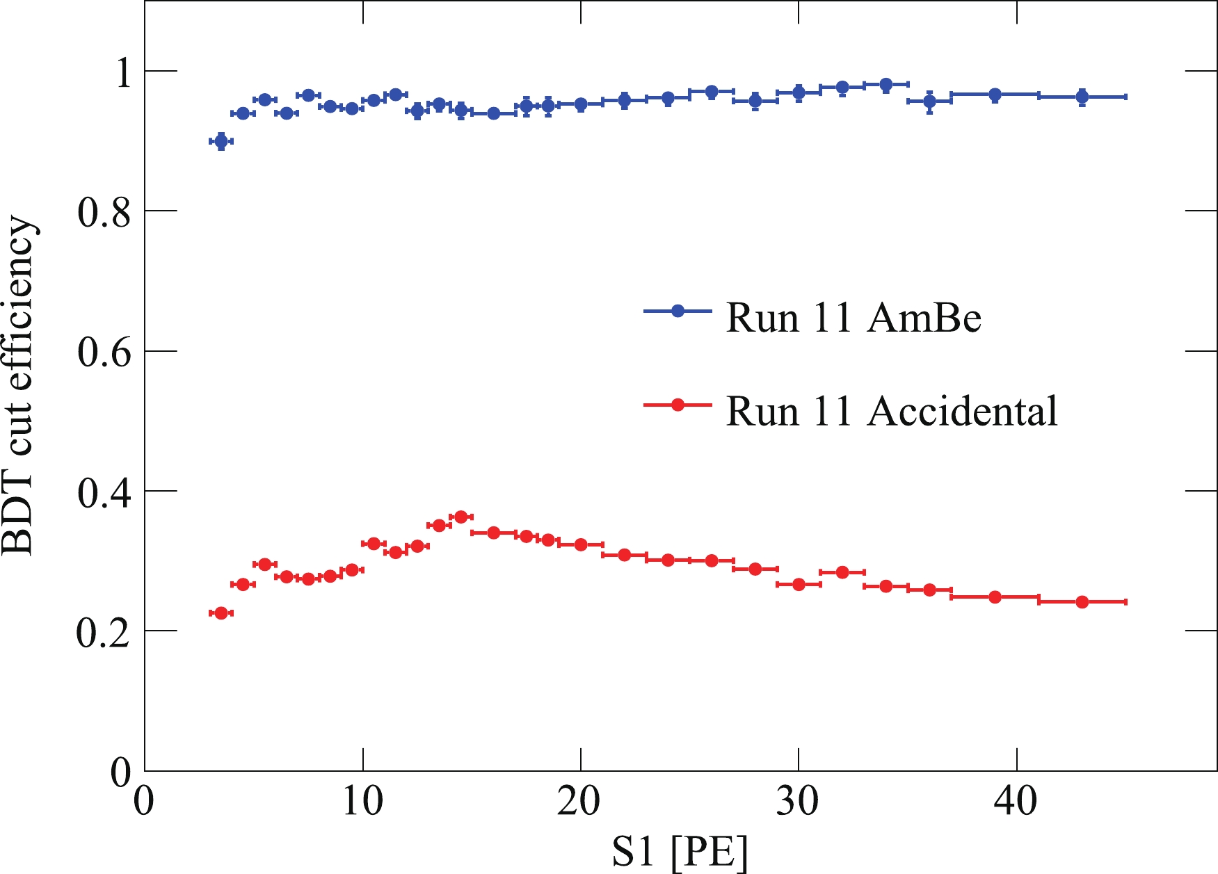
Figure 11. (color online) BDT efficiency
$ \epsilon_{\rm{BDT}} $ and the suppression ratio of accidental background vs.$ S1 $ for Run 11.The
$ \beta $ -decay of daughter$ ^{210} {\rm{Pb}}$ (T$ _{1/2} $ = 22.2 y) on the PTFE surface is observed, presumably due to the$ ^{220} {\rm{Rn}}$ plate-out. These events have a characteristic suppressed$ S2 $ , likely caused by the charge loss onto the PTFE wall during the drift. We also observe a temporal increase of the surface background (events that are reconstructed very close to, or outside, the PTFE wall). A data-driven surface background model [30] is developed to estimate the surface background in the present analysis. Events with$ S1>50 $ PE are used to model the radial distribution of surface events related to$ S2 $ , serving as a shape template in ($ R^2, S2 $ ). The background is then normalized by the DM data outside the FV. A comparison between the scaled template and data along$ R^{2} $ is shown in Fig. 12. The number of events below the$ -4\sigma $ line of the ER band in the data (model) with$ S1\in(50,100) $ and$ R^2\in (0,720) $ cm2 is 20 (17.4) in Run 9, 28 (31.6) in Run 10, and 187 (161.8) in Run 11, with the same quality cuts for DM events applied. The model uncertainty is estimated to be 20% due to the resolution of 5 mm in the position reconstruction. The expected number of surface events in the DM search region is$ 2.9\pm0.6 $ ,$ 3.6\pm{0.8} $ , and$ 15.4\pm{3.3} $ events in Runs 9, 10, and 11, respectively.
Figure 12. (color online) (a) and (b): Comparison between the
$ R^{2} $ distribution of surface events (dots) and model predictions (lines) for Run 9 (blue), Run 10 (magenta), and Run 11 (green). (c) The$ \log_{10}(S2/S1) $ vs.$ S1 $ band for events outside the FV. The median of the ER band (black dashed line) and the NR band (red dashed line) and$ -4\sigma $ of the ER and (blue dashed line) are overlaid. -
Due to blind analysis, the selection cuts for final candidates are set without considering the real data for Run 11. The signal window to search for DM candidates and the fiducial radius are optimized by requiring the best DM sensitivity at the mass of 40 GeV/
$ {\rm c}^2 $ , with a below-NR-median (BNM) signal acceptance, within which the background is evaluated with a cut-and-count approach. For$ S1 $ , we inherit the range of$ [3, 45] $ PE as in the previous analysis, asthe sensitivity flattens for upper cuts from 45 to 70 PE. As was done previously,$ S2 $ is selected between 100 (raw) and 10000 PE, together with the 99.99% NR acceptance line and an additional 99.9% ER acceptance cut to eliminate a few events with unphysically large sizes of$ S2 $ . All runs share the same selection cuts on the fiducial radius, i.e.,$ R^2<720\; \rm{cm}^2 $ . The range of the drift time is determined to be$ (18,310) $ μs in Run 9, and$ (50,350) $ μs in Runs 10 and 11 (lower cut is higher than that in Ref. [6]), based on the vertical distribution of events with$ S1 $ between 50 and 70 PE. The xenon mass within the FV is estimated to be$ 328.9\pm9.9 $ kg in Run 9 and$ 328.6\pm9.9 $ kg in Runs 10 and 11, where the uncertainties are estimated using a 5-mm resolution in the position reconstruction. The final exposures used in this analysis are 26.2 ton$ \cdot $ day in Run 9, 25.3 ton$ \cdot $ day in Run 10, and 80.3 ton$ \cdot $ day in Run 11.The number of events in the DM search data passing the cuts is summarized in Table 4. In total, 1222 candidates are obtained in the three runs. A post-unblinding event-by-event waveform check is then performed, in which two spurious events in Run 11 are identified (detailed waveforms are shown in Appendix A). One event is a double
$ S2 $ event, as shown in Fig. A1, with a second small$ S2 $ being split into a few$ S1 $ s in our clustering algorithm, which are, therefore, not properly registered. The other event has a small$ S1 $ formed by three coincidental PMT hits, but two of the hits are due to coherent noise pickup, shown in Fig. A2. The final number of candidates is 1220. The sequential reduction of events after various cuts is summarized in Table 4.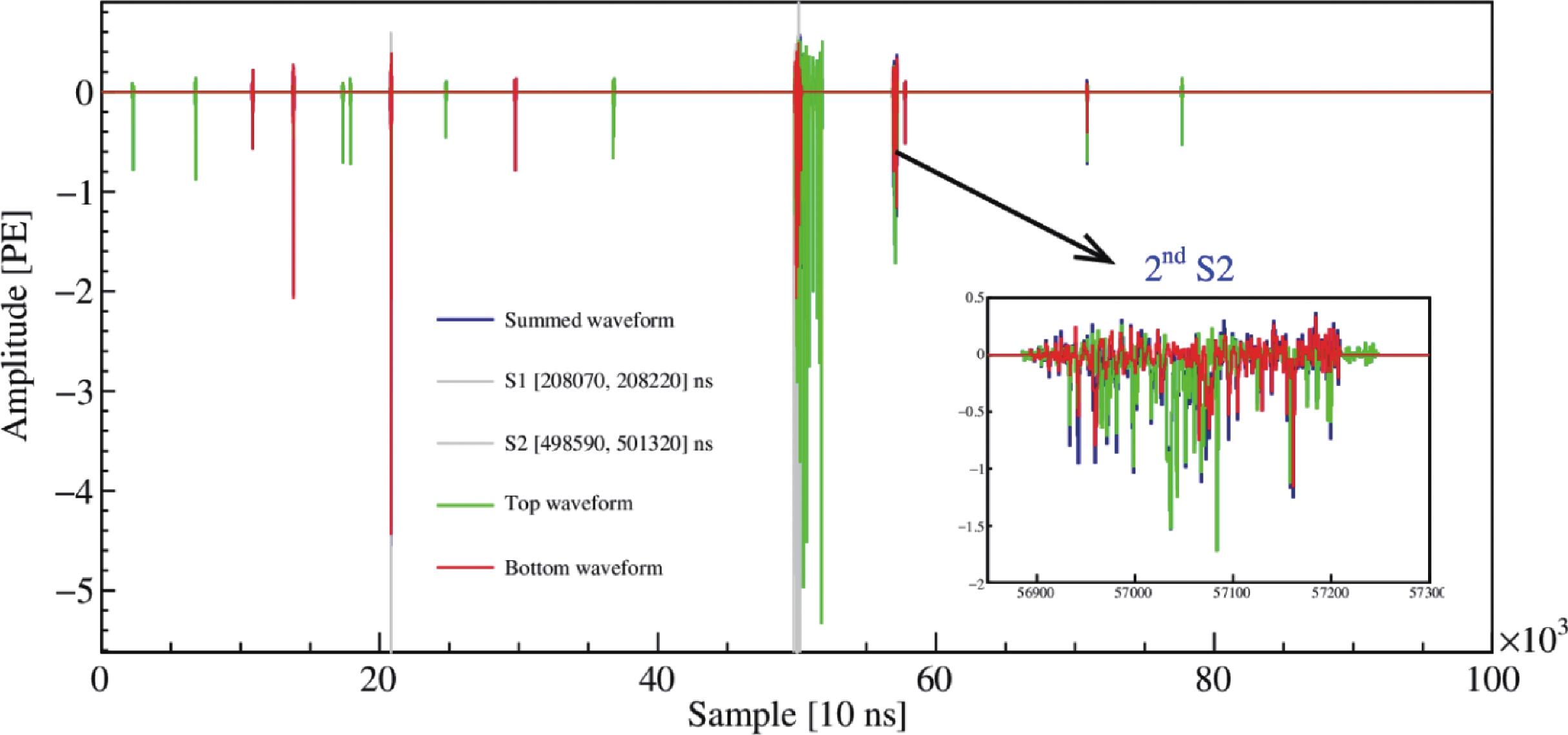
Figure A1. (color online) The full waveform of event 167193 in run 20922. The second small
$ S2 $ was split into a few$ S1 $ s in our clustering algorithm, so that it was incorrectly recognized as a single scattering events.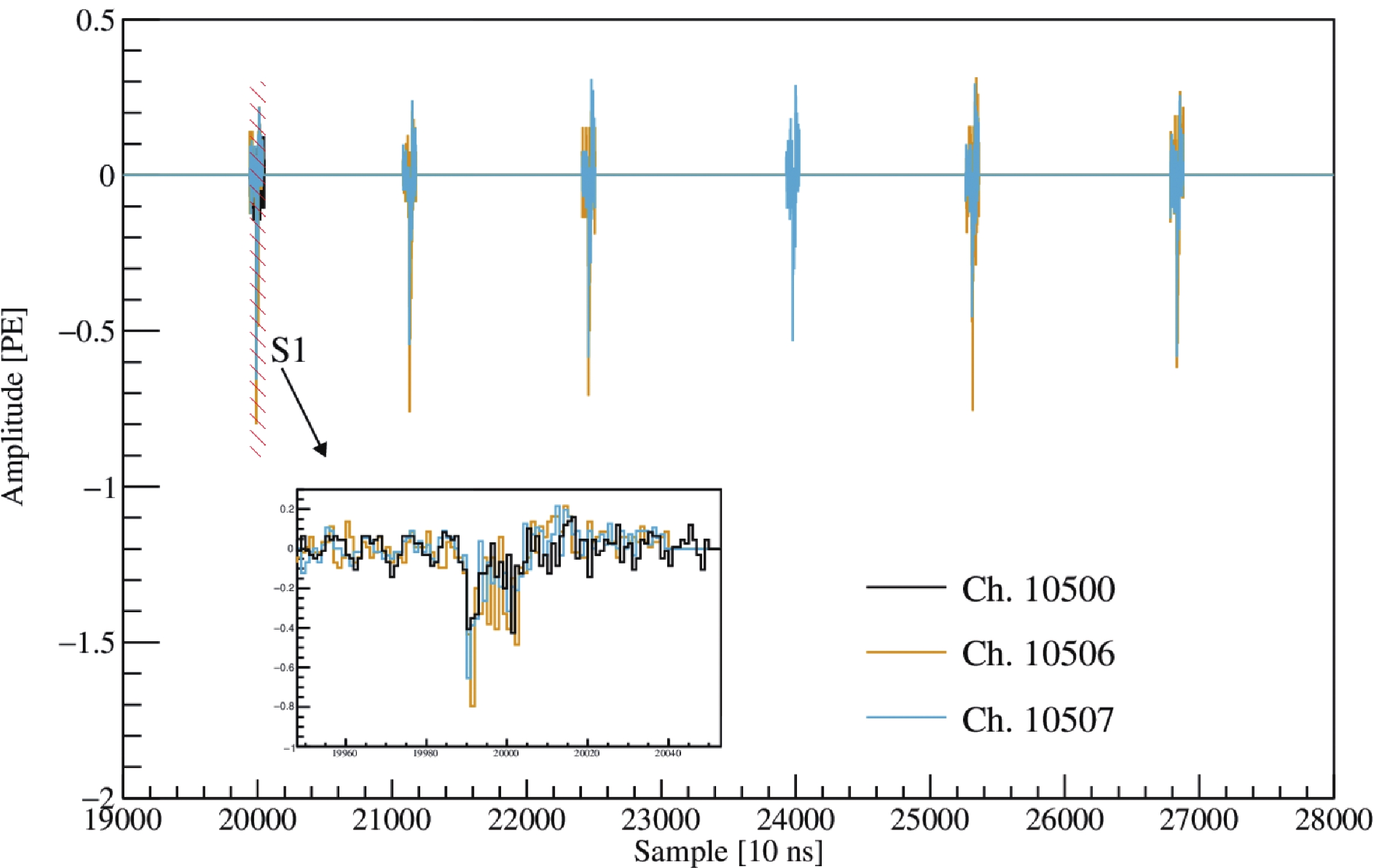
Figure A2. (color online) The partial waveform of event 112727 in run 22940. Two of the three hits in the reconstructed
$ S1 $ are due to the coherent noise pickup in channel 10506 and 10507.The spatial distribution of events inside and outside the FV (in the same
$ S1 $ and$ S2 $ selection region) is shown in Fig. 13. In Run 11, more events are clustered to the wall, consistent with the increase of the surface background.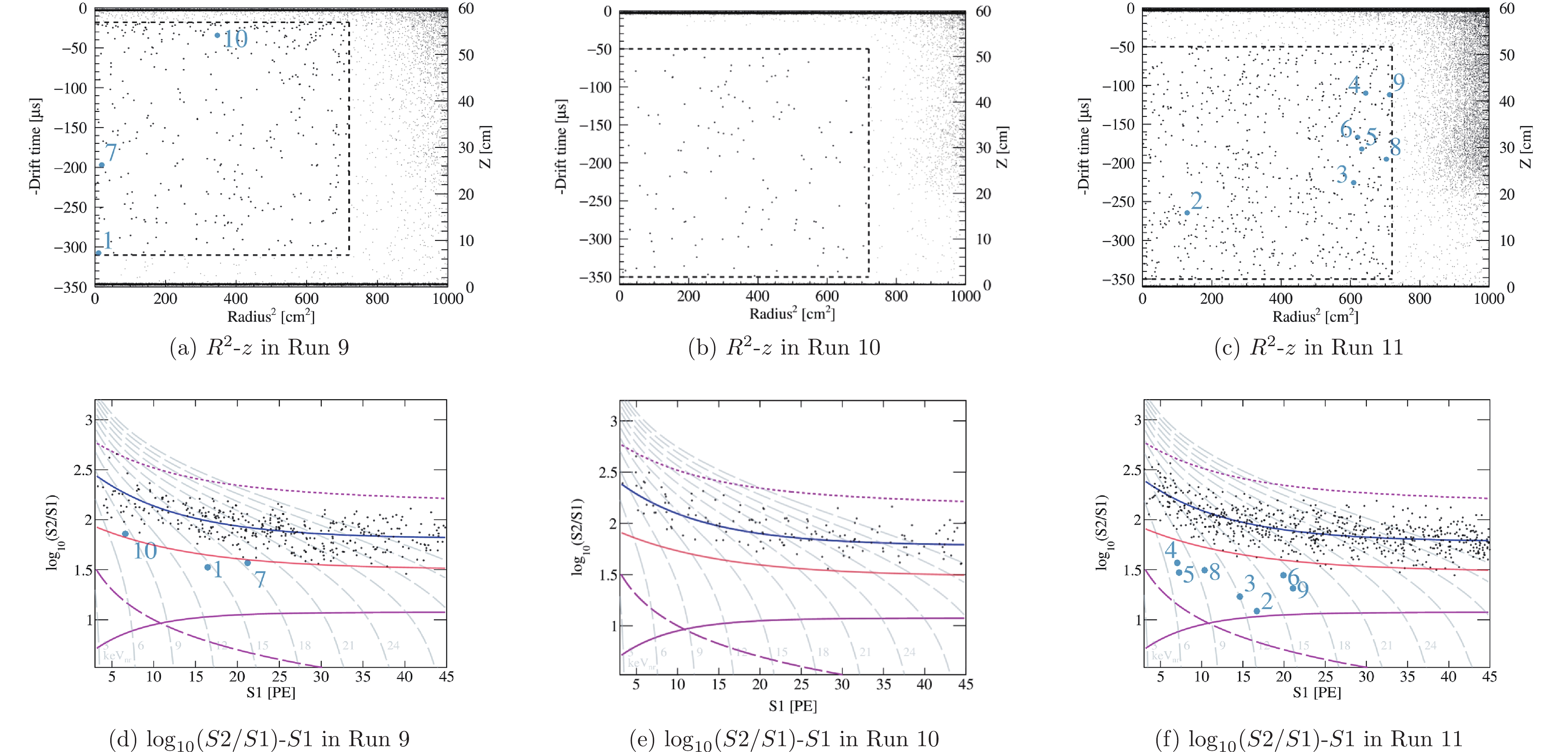
Figure 13. (color online) The spatial and signal distributions of events within
$ S1 $ and$ S2 $ range cuts. The events outside the FV are also presented for Run 9(a), Run 10(b), and Run 11(c). Only the final candidates in the DM search data are shown on the signal distributions for Run 9(d), Run 10(e), and Run 11(f). The ten most likely DM candidates are labeled. References of the ER band median (blue solid line) and NR band median (pink solid line) are shown in the signal distributions. The magenta lines are the boundaries of the acceptance window. The solid and dotted magenta lines are the 99.99% NR and 99.9% ER acceptance cuts, respectively. The dashed magenta line is the$ S2 = 100 $ PE boundary. The dashed grey curves represent the equal-energy curves in nuclear recoil energy (keV$ _{\rm NR} $ ).The distributions of the candidate events in
$ \log_{10}(S2/S1) $ vs.$ S1 $ for the three runs are also shown in Fig. 13, with NR median lines shown for reference. The number of BNM candidates in Runs 9, 10, and 11 are 4, 0, and 34, respectively. Although the statistical interpretation of the data is given in Sec. 7, we discuss some general features here. One of the BNM events in Run 9 was the same in the previous analysis [3], with$ S1\sim $ 40 PE and$ R^2\sim330 $ cm2. Another three appear reasonably close to the center of the TPC, which was above the NR-median in the previous analysis, but appears as BNM after the improved uniformity correction. The majority of the BNMs in Run 11 are consistent with the surface background and the ER background. For example, if we reduce the maximum radius cut to$ R^2<600 $ cm2 in Run 11, the BNMs decrease to 14, with 11 of them quite close to the NR median. A comparison between the observed candidates and the expected background is given in Table 5, and the best fit background values (see Sec. 7) are also given in the table. From a simple cut-and-count point of view, no significant excess is found above the background.ER Accidental Neutron Surface Total fitted Total observed Run 9 381.1 2.20 0.77 2.13 $ 387\pm23 $ 

384 below NR median 2.7 0.46 0.37 2.12 $5.6\pm 0.5$ 

4 Run 10 141.7 1.08 0.48 2.66 $145.9\pm16$ 

143 below NR median 1.7 0.24 0.22 2.65 $4.8\pm 0.6$ 

0 Run 11, span 1 216.5 1.04 0.60 6.24 $224\pm 22$ 

224 below NR median 4.2 0.32 0.32 6.22 $11.1\pm 1.1$ 

13 Run 11, span 2 448.2 1.60 0.92 9.58 $460\pm35$ 

469 below NR median 8.26 0.50 0.50 9.54 $18.8\pm 1.7$ 

21 Total 1187.9 5.9 2.77 20.6 $1217\pm60$ 

1220 below NR median 16.8 1.52 1.42 20.5 $40.3\pm3.1$ 

38 Table 5. The best fit total and below-NR-median background events in Run 9, Run 10 and Run 11 in the FV with the signal model
$ m_{\chi} = 400 $ GeV/$ {\rm c}^2 $ . The BNM backgrounds are estimated with the PDFs. The nuisance parameters can be found in Table 6, the uncertainties of which are propagated into the total fitted event uncertainties. Numbers of observed events are shown in the last column. -
The statistical interpretation of the data is carried out using a profile likelihood ratio (PLR) approach, very similar to the treatment in Refs. [3, 6, 31]. For the ER background, except for
$ ^{127} {\rm{Xe}}$ and tritium, the others are mostly flat within the region of interest. We combine them into a single “flat ER background” to avoid degeneracy in the likelihood fit. The unbinned likelihood function is constructed as$\begin{split}{{\cal L}_{{\rm{pandax}}}} =& \left\{ {\prod\limits_{n = 1}^{{\rm{nset}}} {\left[ {{\rm{Poiss}}({\cal N}_{{\rm{obs}}}^n|{\cal N}_{{\rm{fit}}}^n) \times \prod\limits_{i = 1}^{{\cal N}_{{\rm{obs}}}^n} {(l_s^{n,i} + \sum\limits_b {l_b^{n,i}} )} } \right]} } \right\} \\&\times \left[ {G({\delta _s},{\sigma _s})\prod\limits_b G ({\delta _b},{\sigma _b})} \right],\end{split}$

(4) with
$ {\cal N}_{\rm{fit}}^{n} = N_s^n(1+\delta_s) + \sum\limits_bN_b^n(1+\delta_{b}), $

(5) $l_{s}^{n,i} = \frac{N_s^n(1+\delta_s)P_{\rm DM}^n(S1^i,S2^i,r^i,z^i)}{{\cal N}_{\rm{fit}}^{n}}, $

(6) $ l_{b}^{n,i} = \frac{N_{b}^n(1+\delta_{b})P_{b}^n(S1^i,S2^i,r^i,z^i)}{{\cal N}_{\rm{fit}}^{n}},$

(7) $ G(\delta, \sigma) = \frac{1}{\sqrt{2\pi}\sigma}\exp\left(-\frac{\delta^{2}}{2\sigma^2}\right).$

(8) Instead of simply dividing the data into three runs, we separated the data into 14, 4, and 6 sets in Runs 9, 10, and 11 (so n runs up to 24), respectively, according to different operating conditions, such as the drift/extraction fields and electron lifetime, which affect the expected signal distributions. For each set, the number of observed events is
$ {\cal N}_{\text{obs}}^n $ ;$ N_s^n $ and$ N_b^n $ are the number of signal and backgrounds events, respectively. In this analysis,$ N_s^n $ is related to the DM-nucleon cross-section$ \sigma_{\chi n} $ by the incoming flux (standard halo), the number of target xenon nuclei, and the Helms form factor [32]. The nuisance normalization parameters$ \delta_s $ and$ \delta_b $ are constrained by the uncertainties$ \sigma_s $ and$ \sigma_b $ , respectively, by a Gaussian penalty function$ G(\delta,\sigma) $ .$ \sigma_s $ is set to be 20% to capture the global uncertainties in the DM flux, target mass, and detector efficiency, and$ \sigma_b $ is obtained from Table 3. For$ ^{127} {\rm{Xe}}$ , accidental, and neutrino backgrounds, in all data sets we assume a common$ \delta_b $ to reflect the correlated systematic uncertainty. On the other hand, the flat ER and surface backgrounds have independent values of$ \delta_b $ to reflect the set-to-set changes. The tritium background is left to float in the fit (no corresponding penalty).The PDFs for signals and backgrounds,
$ P_s^n $ and$ P_{b}^n $ , are extended to four dimensions ($ S1 $ ,$ S2 $ , r, z). Except for the surface background, the signal distributions of DM and other backgrounds are treated to be independent from their spatial distributions. The spatial distributions of neutron and$ ^{127} {\rm{Xe}}$ backgrounds are extracted from Geant4-based simulations, and that for the accidental background is obtained from random isolated-$ S1 $ -$ S2 $ pairs. The four-dimensional distribution of the surface background is produced with the data-driven surface model [30], within which$ S1 $ ,$ S2 $ , and r are correlated (see Fig. 12), and z is independent. Spatial distributions of all other backgrounds and DM signals are uniform. The ER background PDF in$ S1 $ and$ S2 $ follows the NEST2-based modeling in Sec. 4.4. The DM signal PDF is obtained by assuming a standard halo model and an NR energy spectrum of the spin-independent (SI) elastic DM-nucleus scattering used in previous analyses [3, 6, 8], together with the updated NR model mentioned earlier. The selection efficiency is embedded in the PDF, by generating events weighted by the overall efficiency (Eq. (1)). The detection efficiency for NR events as a function of the recoil energy is illustrated in Fig. 14.
Figure 14. (color online) The detection efficiencies as functions of the NR energy for Run 9 (blue), Run 10 (magenta), and Run 11 (green).
Standard fitting is performed on the combined data to minimize the PLR test statistic (
$ q_{\sigma} $ ) at different DM masses$ m_{\chi} $ . The best fit of DM events for$ m_{\chi}>200 $ GeV/$ {\rm c}^2 $ is almost the same as the best fit of nuisance parameters in Table 6. As an example, for$ m_{\chi} = 400 $ GeV/$ {\rm c}^2 $ , the best fit of$ \sigma_{\chi n} $ is$ 4.4\times 10^{-46} $ cm$ ^{2} $ , corresponding to a detected signal number of 5.7. Based on the background-only toy Monte Carlo tests, the best fit corresponds to a p-value of 0.17, which is equivalent to a significance of 0.96$ \sigma $ , consistent with no significant excess above the background.$ m_{\chi}=400 \;{\rm{GeV}}/ {\rm c}^2$ 

$ \delta_{^3{\rm{H}}} $ 

$ -0.03\pm0.27 $ 

$ {\delta _{{\rm{flat}}\;{\rm{ER}},\;{\rm{Run}}\;{\rm{9}}}} $ 

$ -0.08\pm0.07 $ 

${\delta _{{\rm{flat}}\;{\rm{ER}},\;{\rm{Run}}\;{\rm{10}}}}$ 

$0.02\pm0.13$ 

${\delta _{{\rm{flat}}\;{\rm{ER}},\;{\rm{Run}}\;{\rm{11}},\;{\rm{span}}\;{\rm{1}}}}$ 

$0.08\pm0.11$ 

${\delta _{{\rm{flat}}\;{\rm{ER}},\;{\rm{Run}}\;{\rm{11}},\;{\rm{span}}\;{\rm{2}}}}$ 

$0.10\pm 0.08$ 

$ \delta_{^{127}{\rm {Xe}}} $ 

$ 0.00\pm 0.13 $ 

$ \delta_{\rm{accidental}} $ 

$0.02\pm 0.29$ 

$ \delta_{\rm{neutron} }$ 

$ -0.04\pm0.49 $ 

${\delta _{{\rm{wall}}\;{\rm{Run}}\;{\rm{9}}\;{\rm{and}}\;{\rm{10}}}}$ 

$ -0.26\pm0.20 $ 

${\delta _{{\rm{wall}}\;{\rm{Run}}\;{\rm{11}}}}$ 

$ 0.03\pm0.16 $ 

Table 6. The best fit nuisance parameters for
$ m_{\chi} = 400 $ GeV/$ {\rm c}^{2} $ .We also examine the likelihoods (Eqs. (6) and (7)) of individual events using backgrounds and DM PDFs. For the top ten DM-like events with
$ m_{\chi} = 400 $ GeV/$ {\rm c}^{2} $ labeled in Fig. 13, the ratios of the likelihoods of different hypotheses for each event are presented in Fig. 15. This confirms our observations that out of the 38 BNM events, most of them are likely to be a surface background or an ER background. Events 1 and 2 have the highest probability of being either a DM or accidental background.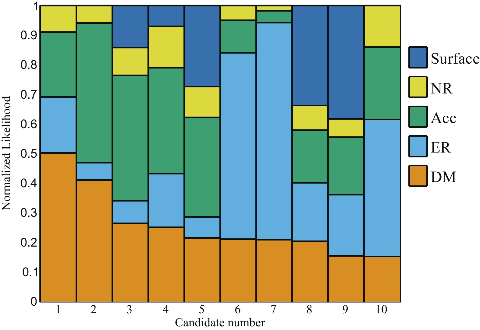
Figure 15. (color online) The normalized likelihoods of the most likely DM events for
$ m_{\chi} = 400 $ GeV/$ {\rm c}^{2} $ .Based on the above, we choose to report the upper limit of the cross section of this search. The standard CL
$ _{s+b} $ approach [33] is adopted, for which we performed a two-dimensional scan in ($ m_{\chi} $ ,$ n_{\chi n} $ ). On each grid, a large number of toy Monte Carlo simulations with similar statistics are generated and fitted with the signal hypothesis, with the resulting distribution of$ q_{\sigma,{\rm MC}} $ compared to the observed$ q_{\sigma,{\rm data}} $ to define the 90% confidence level of the exclusion. The results below 10 GeV/$ {\rm c}^2 $ are power constrained at$ -1\sigma $ of the sensitivity band [34], which is obtained by generating 90% exclusion lines using background-only Monte Carlo simulation data sets, with the same PLR procedures. The results are shown in Fig. 16. The minimum excluded$ \sigma_{\chi n} $ is$ 2.2\times10^{-46} $ cm2 at$ m_{\chi} $ of 30 GeV/$ {\rm c}^2 $ , corresponding to a detected DM number of 1.7. At higher masses, the limit is set at$ 2.5\times10^{-46} $ ($ 1.6\times10^{-45} $ ) cm2 for a WIMP mass of 40 (400) GeV/$ {\rm c}^2 $ , and the corresponding number of detected DM signal events is 11.6 (18.4). The limit curve is weakened from that in Ref. [6], in which a downward fluctuation of the background was observed and the limit was power-constrained to -1$ \sigma $ . The turning of the limit curve around 15 GeV/c2 is due to the fact that the most "DM-like" events have$ S1>10 $ PE (see Fig. 13); thus, their DM-likelihoods increase with increasing WIMP mass after roughly 15 GeV/c2.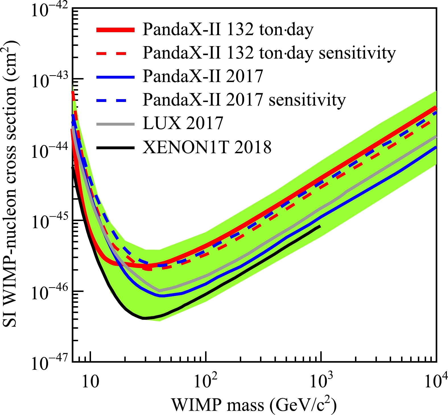
Figure 16. (color online) The 90% confidence level upper limits vs.
$ m_{\chi} $ for the spin-independent WIMP-nucleon elastic cross sections from the full exposure data of PandaX-II (red), overlaid with that from PandaX-II 2017 [6], LUX 2017 [4], and XENON1T 2018 [7]. The green band represents the$ \pm1\sigma $ sensitivity band. Below 8 GeV/c2, the median sensitivity of this analysis is slightly weaker than that in 2017, as our nuclear recoil model is re-calibrated, leading to a lower signal efficiency for low mass WIMPs. -
In summary, we report the WIMP search results with the 132 ton
$ \cdot $ day full exposure data of the PandaX-II experiment, which include a combination of data corresponding to 401 live-days with several running conditions. Several major improvements have been made in the data correction, selection, signal modeling, and data fitting in this analysis. No significant excess of events is identified above the background. A 90% upper limit is set on the SI elastic DM-nucleon cross section with the lowest excluded value of$ 2.2\times10^{-46} $ cm2 at a WIMP mass of 30 GeV/$ {\rm c}^2 $ .The long duration of the PandaX-II operation, the systematic studies performed, and the analysis techniques are all crucial for the development of the next generation of PandaX programs, i.e., PandaX-4T [35]. With the four-ton scale of a sensitive liquid xenon target in a lower-background detector, the PandaX-4T experiment is under preparation in the second phase of CJPL (CJPL-II). Together with worldwide multi-ton scale experiments, [36, 37], the sensitivity of the DM search will be advanced by more than one order of magnitude in the near future.
We thank the Key Laboratory for Particle Physics, Astrophysics and Cosmology, Ministry of Education, for important support. This work was supported in part by the Chinese Academy of Sciences Center for Excellence in Particle Physics (CCEPP), and the Hongwen Foundation in Hong Kong. Finally, we thank the CJPL administration and the Yalong River Hydropower Development Company Ltd. for the indispensable logistical support and other help.
Results of dark matter search using the full PandaX-II exposure
- Received Date: 2020-07-26
- Available Online: 2020-12-01
Abstract: We report the dark matter search results obtained using the full 132 ton·day exposure of the PandaX-II experiment, including all data from March 2016 to August 2018. No significant excess of events is identified above the expected background. Upper limits are set on the spin-independent dark matter-nucleon interactions. The lowest 90% confidence level exclusion on the spin-independent cross section is 2.2 × 10−46 cm2 at a WIMP mass of 30 GeV/c2.


 Abstract
 HTML
HTML Reference
 Related
 PDF
PDF




 DownLoad: