


 Abstract
 HTML
HTML Reference
 Related
 PDF
PDF


-
Two-neutrino double beta (
$ 2\nu\beta\beta $ ) decay is an interesting process (a second-order weak interaction) in the standard model, which was proposed by Mayer [1] in 1935. It is a significant subject in nuclear and particle physics that can be used to test models of the weak interaction [2, 3]. The$ 2\nu\beta\beta $ decays have ultra-long half-lives of over$ 10^{18} $ years [4, 5], which is at least one billion times longer than the age of the universe itself. To date, 90 nuclei are believed to undergo$ 2\nu\beta\beta $ decay, of which only 14 have been measured [6-10]. The complementary experimental information from related$ 2\nu\beta\beta $ decay can improve the quality of nuclear structure models [11]. In addition, research on$ 2\nu\beta\beta $ decay can be used to calculate the nuclear matrix elements (NMEs) of$ 0\nu\beta\beta $ decay as a promising source of$ 0\nu\beta\beta $ decay detection [12]. It is well known that the absolute mass of the neutrino is still a mystery [13, 14]. If$ 0\nu\beta\beta $ decay could be detected, it could settle this problem when combined with the NMEs governed by the theory [15, 16]. Thus, whether experimental or theoretical, research into$ 2\nu\beta\beta $ decay is extremely significant.The role of accurate NMEs in
$ 2\nu\beta\beta $ decay cannot be underestimated [17]. Although the NMEs between the initial and final nuclei ground states have been investigated using several approaches [18-24], they are still notoriously difficult to calculate, as shown in Eq. (1) [25]:$ M_{2\nu } = \sum\limits_{n}\frac{\left\langle 0_{f^{+}}\left\Vert \sum_{i}\sigma\left( i\right)\tau ^{\pm }\left( i\right) \right\Vert1_{n}^{+}\right\rangle \left\langle 1_{n}^{+}\left\Vert\sum_{i}\sigma\left( i\right) \tau ^{\pm }\left( i\right) \right\Vert0_{i^{+}}\right\rangle }{\left[ \frac{1}{2}Q+E\left( 1_{n}^{+}\right) -M_{i}\right] /m_{e}+1}. $

(1) Here, the transition operators are the ordinary Gamow-Teller operators;
$ E\left( 1_{n}^{+}\right) -M_{i} $ denotes the energy discrepancy of the nth intermediate$ 1^{+} $ state and the parent nucleus; and the sum$ \sum_{i} $ extends over all the intermediate$ 1^{+} $ states [25], which poses a challenge in calculations for many nuclei.In recent years, research has been renewed on the single state dominance (SSD) for
$ 2\nu\beta\beta $ decay, which suggests that the lowest intermediate$ 1^{+} $ state dominates the decay [26, 27]. To date, evidence of the SSD for$ ^{82} $ Se has been established by the CUPID-0 collaboration [28]. One of its proven benefits is that the corresponding NMEs can be obtained through single$ \beta $ decay measurements [29]. However, the SSD of many nuclei violates this benefit, with the result that the relevant NMEs cannot be easily determined experimentally. It would hopefully be simpler to calculate only the lowest$ 1^{+} $ wave function instead of all wave functions in the theoretical description [29]. It is thus of great importance to discuss the number of least intermediate$ 1^{+} $ states that saturate the final magnitude.In our work, calculations for six nuclei (
$ ^{36} $ Ar,$ ^{46} $ Ca,$ ^{48} $ Ca,$ ^{50} $ Cr,$ ^{70} $ Zn, and$ ^{136} $ Xe) in a mass range from$ A = 36 $ to$ A = 136 $ are performed within the nuclear shell model (NSM) framework. Calculations are presented for the half-lives, NMEs,$ G_{2\nu} $ , and convergence of the NMEs. In addition, we predict the half-lives of the$ 2\nu\beta\beta $ decays for four nuclei. Relatively short half-lives are predicted for the nuclei$ ^{46} $ Ca and$ ^{70} $ Zn, providing a reference for future experimental detection. Convergence of the NMEs for$ 2\nu\beta\beta $ decays is systematically discussed by analyzing the number of contributing intermediate$ 1^{+} $ states ($ N_{\rm{C}} $ ) for the nuclei of interest. A unified criterion for analyzing$ N_{\rm{C}} $ involved in$ 2\nu\beta\beta $ decay is proposed and adopted. According to the calculations, the general law for convergence of the NMEs for$ 2\nu\beta\beta $ decays is then presented. -
The
$ 2\nu\beta\beta $ decays can be classified into two types: double$ \beta^{-} $ decay (2$ \nu2\beta^{-} $ ) and the decays on the double$ \beta^{+} $ side, i.e., 2$ \nu2\beta^{+} $ , 2$ \nu\beta^{+} $ EC, and 2$ \nu $ 2EC (where EC refers to electron capture) [30]. The formulas used for various types of$ 2\nu\beta\beta $ decay transitions differ, which can be seen in Refs. [13, 30, 31]. The associated half-lives, in connection with the phase space factors ($ G_{2\nu }^{\alpha } $ ) and the NME ($ \left\vert M_{2\nu }^{\alpha}\right\vert $ ), can be expressed by Eq. (2) [30]:$ 1/T_{1/2}^{\alpha } = G_{2\nu }^{\alpha }\left\vert M_{2\nu }^{\alpha}\right\vert ^{2}, \ $

(2) where
$ \alpha = 2\beta^{-} $ , 2$ \beta^{+} $ ,$ \beta^{+} $ EC, and 2EC are different types of$ 2\nu\beta\beta $ decays [13, 30, 31]. The related NME description of the full$ \beta $ strength functions of both the parent and grand nuclei is given [2]. Although formulas for$ G_{2\nu }^{\alpha } $ and$ \left\vert M_{2\nu }^{\alpha }\right\vert $ are supplied by the theory, the calculation for$ \left\vert M_{2\nu }^{\alpha }\right\vert $ is more difficult than that for$ G_{2\nu }^{\alpha } $ because it requires the precise nuclear many-body wave function [32]. The NME is defined in Eq. (1): accurate knowledge of the ground-state for the parent and grand-daughter nuclei, along with all the$ 1^{+} $ states of the intermediate nucleus, clearly plays an important role in evaluations of the NMEs [16].Detailed expressions for various modes of
$ G_{2\nu }^{\alpha } $ can be found in Ref. [33]. The expression is an integral in the phase space of lepton variables; the corresponding values depend on the coupling constant$ g_{A} $ and can be calculated exactly [25, 33]. There is a global effort to address the challenge of the$ g_{A} $ factor. This study applies the commonly used value of$ g_{A} = 1.27 $ , which is consistent with that published in Refs. [13, 17, 34]. -
The calculations for six nuclei (
$ ^{36} $ Ar,$ ^{46} $ Ca,$ ^{48} $ Ca,$ ^{50} $ Cr,$ ^{70} $ Zn, and$ ^{136} $ Xe) are computed in full 1$ \hbar\omega $ shell model spaces without any truncation. Columns 1 and 2 in Table 1 list the nuclei of interest and their shell model spaces, in which the calculations are conducted. To improve the reliability of the calculations, different effective interactions (EIs) are adopted and listed in Column 3. For the$ 2\nu\beta\beta $ decay of$ ^{36} $ Ar, the specific interactions CWH and W are adopted, where the CWH EI is determined by an iterative least squares fit to experimental level energy data [35]; W EI refers to the two-body matrix elements derived from a linear fit [35, 36]. We use the shell model empirical interaction GXFP1A for the$ fp $ shell, which provides 195 two-body matrix elements and 4 single-particle energy subsets through a fit to 699 energy observations within the mass interval$ A = 47-66 $ [37, 38]. Another interaction, KB3, is used to compute the lowest wave function from the full Hamiltonian, with parts of the two-nucleon EI turned off in proper order [39, 40]. It is reasonable to adopt these EIs for the calculations because the concerned nuclei are not far from these regions. We also use the large-scale shell-model interaction SN100PN [41] in the case of$ ^{136} $ Xe, which is obtained from the free nucleon-nucleon CD-Bonn interaction. The interaction is composed of four parts: neutron-neutron, neutron-proton, proton-proton, and Coulomb repulsion between the separate protons [42].Nucleus Shell model space EI $N_{\rm{T}}$ 

$N_{\rm{.cal}}$ 

q $^{36}$ Ar

$sd\left( 0d_{5/2},0d_{3/2},1s_{1/2}\right) $ 

CWH, W 66 66 0.77 [35] $^{46}$ Ca

$fp\left( 1f_{7/2},2p_{3/2},1f_{5/2},2p_{1/2}\right)$ 

GXFP1A, KB3 2361 2361 0.74 [45] $^{48}$ Ca

$fp\left( 1f_{7/2},2p_{3/2},1f_{5/2},2p_{1/2}\right)$ 

GXFP1A, KB3 9470 2000 0.74 [45] $^{50}$ Cr

$fp\left( 1f_{7/2},2p_{3/2},1f_{5/2},2p_{1/2}\right)$ 

GXFP1A, KB3 383932 2000 0.74 [45] $^{70}$ Zn

$fp\left( 1f_{7/2},2p_{3/2},1f_{5/2},2p_{1/2}\right)$ 

GXFP1A, KB3 18571 2000 0.68 [46] $^{136}$ Xe

$gdsh\left( 0g_{7/2},1d_{5/2},1d_{3/2},2s_{1/2},0h_{11/2}\right) $ 

SN100PN 16642 2000 0.45 [16] Table 1. Details of the NSM calculations for
$2\nu\beta\beta$ decays.The calculations of the wave functions for the involved nuclei use the diagonalization computer program NuShellX [43]. Columns 4 and 5 provide the total number of intermediate
$ 1^{+} $ states ($ N_{\rm{T}} $ ) and the number of calculated intermediate$ 1^{+} $ states ($ N_{\rm{.cal}} $ ), respectively. One of the most prominent advantages of the NSM is that it considers all the many-body correlations of orbits near the Fermi surface [44], but in theory, the expected total intensity is systematically greater than the observed total intensity [16, 35]. One reliable method of overcoming this problem is to correct the calculated strengths with quenching factors (q), which are tabulated in Column 6. In this article, we apply the widely used values$ q = 0.77 $ for$ A = 16-40 $ ,$ q = 0.74 $ for$ A = 40-50 $ , and$ q = 0.68 $ for$ A = 60-80 $ [35, 45, 46]. For the$ ^{136} $ Xe nucleus,$ q = 0.45 $ [16] is adopted.This research is inseparable from the precise description of wave functions of intermediate states. To test the reliability of the wave functions of the NSM, we compare the first few theoretical energy levels and the
$ \gamma $ -decay half-lives of$ ^{36} $ Cl (the intermediate nucleus for the$ 2\nu\beta\beta $ decay of$ ^{36} $ Ar) in Fig. 1 together with the available experimental information. The theoretical results are obtained with W interaction. As depicted in Fig. 1, the energy levels of the low excited states and most$ \gamma $ -decay half-lives are in good agreement with the experimental data. Thus, within the applicable range, the calculations of the NSM are relatively accurate.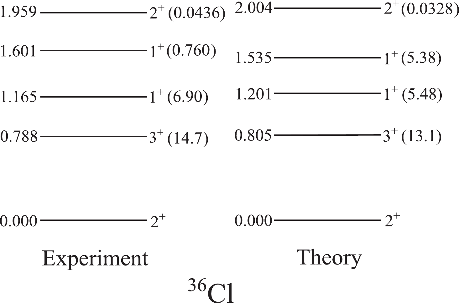
Figure 1. Comparison of the theoretical spectrum of
$^{36}$ Cl and the associated$\gamma $ -decay half-lives with the experimental data. The excitation energies of the states are given in units of MeV and the$\gamma $ -decay half-lives in picoseconds. -
We calculate the properties of
$ 2\nu\beta\beta $ decays for six nuclei ($ ^{36} $ Ar,$ ^{46} $ Ca,$ ^{48} $ Ca,$ ^{50} $ Cr,$ ^{70} $ Zn, and$ ^{136} $ Xe) with Q values adopted from AME2016 [47]. The calculated half-lives,$ G_{2\nu} $ , and NMEs are presented in Table 2, together with other results, either from recent experiments [10, 48-51] or theoretical calculations [17, 44, 52, 53]. Most of the calculated results do not differ greatly from the experimental data. For the half-lives of the$ ^{36} $ Ar and$ ^{50} $ Cr nuclei, our results clearly differ from previous results [52]: the reason is that prevoius works adopted$ g_{A} = -1 $ .Nucleus Q value /keV $G_{2\nu} /{\rm{yr}}^{-1}$ 

$\left\vert M_{2\nu }\right\vert_{.1{\rm{st}}}$ 

$\left\vert M_{2\nu }\right\vert$ 

half-life /yr EI this work others $^{36}$ Ar (2

$\nu$ 2EC)

432.59 $1.28\times 10^{-27}$ 

0.00254 0.117 $5.68\times 10^{28}$ 

$1.4\times 10^{29}$ 

[52] CWH 0.0229 0.151 $3.43\times 10^{28}$ 

W $^{46}$ Ca (2

$\nu2\beta^{-}$ )

988.4 $1.24\times 10^{-22}$ 

0.0564 0.0563 $2.54\times 10^{24}$ 

$1.7\times 10^{24}$ 

[53] GXFP1A 0.0305 0.0468 $3.67\times 10^{24}$ 

KB3 $^{48}$ Ca (2

$\nu2\beta^{-}$ )

4268.08 $4.17\times 10^{-17}$ 

0.0219 0.0250 $3.84\times 10^{19}$ 

$\left( 6.4_{-0.006}^{+0.007}\pm_{-0.009}^{+0.012}\right) \times 10^{19}$ 

[10] GXFP1A 0.0183 0.0226 $4.68\times 10^{19}$ 

$\left( 4.3_{-1.1}^{+2.4}\pm 1.4\right) \times 10^{19}$ 

[48] KB3 $^{50}$ Cr (2

$\nu$ 2EC)

1169.6 $1.25\times 10^{-24}$ 

0.0294 0.123 $5.32\times 10^{25}$ 

$>1.3\times 10^{18}$ 

[49] GXFP1A 0.0515 0.124 $5.21\times 10^{25}$ 

$2.1\times 10^{26}$ 

[52] KB3 $^{70}$ Zn (2

$\nu2\beta^{-}$ )

997.1 $3.24\times 10^{-22}$ 

0.0677 0.138 $1.61\times 10^{23}$ 

$\geqslant3.8\times 10^{18}$ 

[50] GXFP1A 0.00577 0.0867 $4.10\times 10^{23}$ 

$1.4(5)\times 10^{23}$ 

[17] KB3 $^{136}$ Xe (2

$\nu2\beta^{-}$ )

2457.8 $4.69\times 10^{-18}$ 

0.00724 0.0186 $6.16\times 10^{20}$ 

$\left( 2.165\pm 0.016\pm 0.059\right) \times 10^{21}$ 

[51] SN100PN $\left( 2.11\pm 0.25\right) \times 10^{21}$ 

[44] Table 2. Summary of the calculations for the
$ 2\nu\beta\beta$ decays of six nuclei.Recently, evidence of the SSD for
$ ^{82} $ Se has been established by the CUPID-0 collaboration [28]. If the SSD is affirmed, then the corresponding NMEs can be obtained through single$ \beta $ decay measurements [29]. Therefore, it is of great significance to analyze the validity of the SSD. Calculated results show that for the$ 2\nu2\beta^{-} $ decays of$ ^{46} $ Ca and$ ^{48} $ Ca, the first intermediate$ 1^{+} $ state contributes significantly to the final NME. However, there is important canceling in the accumulations of the NMEs, as can be seen in Figs. 7 and 10 in Ref. [52]. In these cases, we cannot conclude that the SSD is satisfied. For other nuclei, the sum of the NMEs gains less than 50% of their final NMEs from the first intermediate$ 1^{+} $ state. Therefore, we cannot conclude that the SSD is satisfied for the related nuclei.The key of the theoretical research on
$ 2\nu\beta\beta $ decays is the calculation of the NMEs. Thus, we present the calculated NMEs together with the Q values in Fig. 2. All the data are from Table 2. The figure illustrates the lack of a significant relationship between the NMEs and the Q values. The calculated results from different EIs are consistent with each other, except in the case of$ ^{70} $ Zn, for which the NME using GXFP1A EI is 1.6 times that using KB3.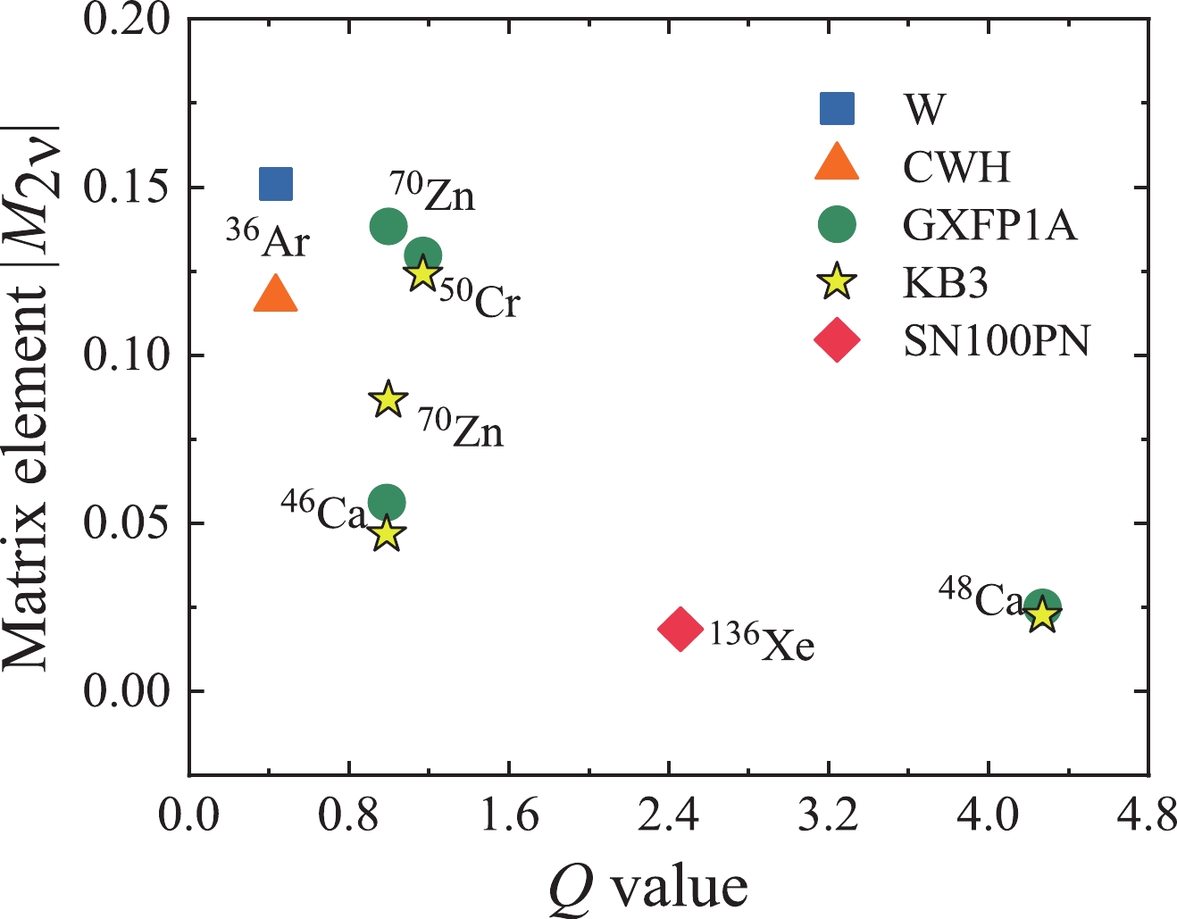
Figure 2. (color online) Comparison of the NMEs for different EIs.
Convergence of the NMEs for
$ 2\nu\beta\beta $ decays is concluded by analyzing the number of contributing intermediate$ 1^{+} $ states ($ N_{\rm{C}} $ ) for the concerned nuclei. We assume that a$ 2\nu\beta\beta $ decay NME is well converged when the accumulated NMEs saturate 99.7% of the final magnitude. This is illustrated in Fig. 3, where for the$ ^{70}{\rm{Zn}}\longrightarrow $ $ ^{70}{\rm{Ge}} $ decay for GXFP1A EI, points A (5th state), B (103rd state), and C (214th state) all satisfy this criterion. Only after point C has satisfied the criterion, indicating that the NME has no distinct twists, is the accumulation believed to be saturated. We thus assume that after point C (214th state), the NME is reliably converged. Accordingly,$ N_{\rm{C}} $ is determined naturally. This criterion is used throughout this article.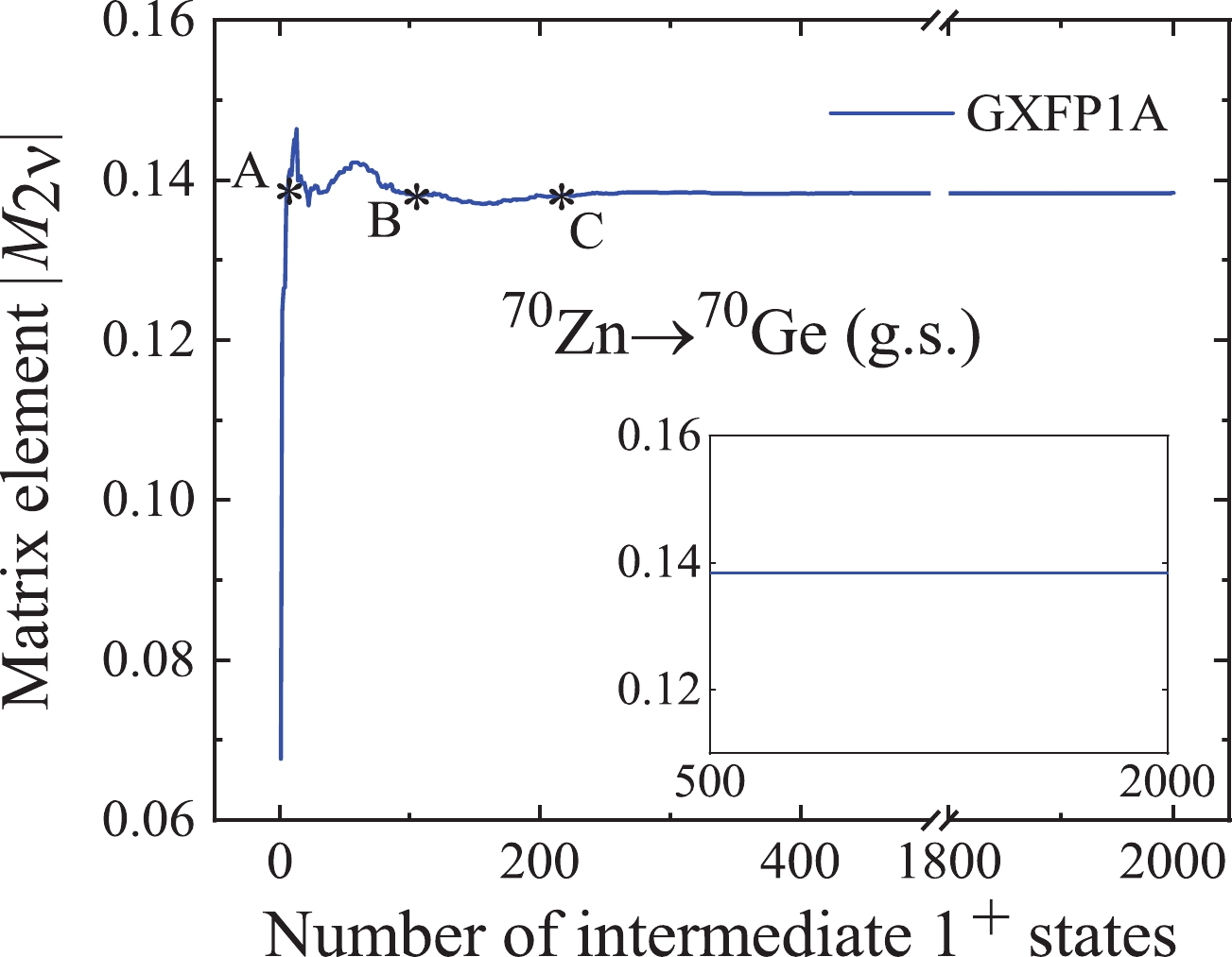
Figure 3. (color online) Accumulations of the NMEs for the
$^{70}{\rm{Zn}}\longrightarrow$ $^{70}{\rm{Ge}}$ decay to ground state.A detailed analysis of the convergence of NMEs based on the above criterion is presented in Table 3 for the nuclei of interest. Notice that the actual contributing excitation energy for
$ ^{136} $ Xe decay is smaller than for the other concerned nuclei (see Column 5), which suggests that the level density is large.Nucleus $N_{\rm{T}}$ 

$N_{\rm{C}}$ 

$N_{\rm{C}}/N_{\rm{T}}$ 

Ex/MeV EI $^{36}$ Ar

66 34 51.5% 33.6 CWH 32 48.5% 36.5 W $^{46}$ Ca

2361 130 5.51% 24.3 GXFP1A 111 4.70% 22.4 KB3 $^{48}$ Ca

9470 150 1.58% 23.4 GXFP1A 183 1.93% 24.7 KB3 $^{50}$ Cr

383932 417 0.109% 22.5 GXFP1A 423 0.110% 23.7 KB3 $^{70}$ Zn

18571 214 1.15% 23.0 GXFP1A 165 0.888% 25.4 KB3 $^{136}$ Xe

16642 1009 6.06% 12.7 SN100PN Table 3. Details of the convergence of NMEs according to the criterion that the accumulated NMEs should saturate 99.7% of the final magnitude.
From the calculations for the involved nuclei, we discover a connection between the total number of intermediate
$ 1^{+} $ states ($ N_{\rm{T}} $ ) and the number of contributing states ($ N_{\rm{C}} $ ). A linear analysis for a general convergence law of the NMEs is depicted in Fig. 4. The unfilled circles represent the CWH and GXFP1A EIs, and the solid circles are for the W, KB3, and SN100PN EIs. All the data are from Table 3. We use a solid line for the fit using five nuclei ($ ^{36} $ Ar,$ ^{46} $ Ca,$ ^{48} $ Ca,$ ^{50} $ Cr, and$ ^{70} $ Zn) and express the correlation between$ N_{\rm{C}} $ and$ N_{\rm{T}} $ by Eq. (3):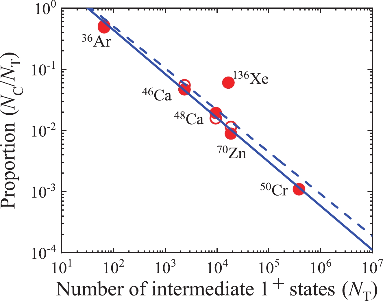
Figure 4. (color online) Correlation between the convergence proportion (
$N_{\rm{C}}/N_{\rm{T}}$ ) in a$\log_{10}$ frame and$N_{\rm{T}}$ in$\log_{10}$ frame. The solid line is a linear fit including all the nuclei except$^{136}$ Xe, and the dashed line is for all the nuclei of interest. The unfilled and solid circles represent the results from different EIs.$ N_{\rm{C}} = \left( 10.8\pm 1.2\right) \times N_{\rm{T}}^{\left( 0.29\pm 0.02\right) }, \ $

(3) with a linear correlation coefficient of 0.996, which is very close to 1. The overall trend of the convergence properties is in good agreement with the correlation, except in the case of the
$ ^{136} $ Xe nucleus, which deviates slightly from the solid line. The reason may be that the level density of$ ^{136} $ Cs (the intermediate nucleus for$ 2\nu\beta\beta $ decay of$ ^{136} $ Xe) is obviously larger than that of the others. For the other nuclei, the excitation energy exceeds 20 MeV up to the 300th intermediate$ 1^{+} $ state, whereas the excitation energy of the 1009th intermediate$ 1^{+} $ state for$ ^{136} $ Cs is only 12.7 MeV, as listed in Table 3. Thus, the$ 2\nu\beta\beta $ decay of$ ^{136} $ Xe is unusual. If the$ ^{136} $ Xe nucleus is taken into account, the correlation is expressed by Eq. (4),$ N_{\rm{C}} = \left( 10.7\pm 2.1\right) \times N_{\rm{T}}^{\left( 0.32\pm 0.08\right) }, \ $

(4) with a linear correlation coefficient of 0.884. Hopefully, the number of least intermediate
$ 1^{+} $ states needed for the precise calculation of NMEs can be obtained from Eq. (3).To check the applicability of Eqs. (3) and (4), two new transitions are performed. One is the
$ ^{64}{\rm{Zn}}\longrightarrow $ $ ^{64}{\rm{Ni}} $ decay computed in the$ fpg $ model space with JUN45 and JJ44B interactions. Details of the calculated results are presented in Table 4. The calculated values of$ N_{\rm{C}} $ are almost identical for the different interactions within the theoretical range of the two equations.Nucleus Shell model space $N_{\rm{T}}$ 

$N_{\rm{C}}$ 

Theoretical $\,{N_{\rm{C}}}$ 

EI Eq. (3) Eq. (4) $^{64}$ Zn

$fpg$ 

12378 182 $167\pm 32$ 

$219\pm 66$ 

JUN45 $fpg$ 

12378 186 $167\pm 32$ 

$219\pm 66$ 

JJ44B $^{68}$ Ni

$fp$ 

18571 205 $187\pm 34$ 

$249\pm 73$ 

GXFP1A $fpg$ 

42895 241 $238\pm 40$ 

$326\pm 89$ 

JUN45 Table 4. Summary of the convergence of the NMEs of new nuclei.
Another transition of interest is the
$ ^{68}{\rm{Ni}}\longrightarrow $ $ ^{68}{\rm{Zn}} $ decay in the$ fp $ and$ fpg $ model spaces. Although this decay does not occur in nature, the related calculations could be used to further discuss the applicability of Eqs. (3) and (4) in different model spaces. In addition, the calculated values of$ N_{\rm{C}} $ for the different model spaces are within the theoretical range of the two equations. Thus, Eqs. (3) and (4) are feasible within the applicable range. We hope our research is useful for shell model calculations in$ 2\nu\beta\beta $ decay. -
In this work, the general features and convergence of the NMEs for the
$ 2\nu\beta\beta $ decays of six nuclei in a mass range from$ A = 36 $ to$ A = 136 $ are studied under the framework of the nuclear shell model (NSM). Different effective interactions (EIs) are adopted to improve the reliability of the calculations. Calculations are presented for the half-lives, NMEs,$ G_{2\nu} $ , and convergence of the NMEs. Most of the results are very close to the experimental data. In addition, we predict the half-lives of$ 2\nu\beta\beta $ decays for four nuclei. The nuclei$ ^{46} $ Ca and$ ^{70} $ Zn have relatively short half-lives, which will hopefully be probed by future experiments.Convergence of the NMEs for
$ 2\nu\beta\beta $ decays is discussed systematically by analyzing the number of contributing intermediate$ 1^{+} $ states ($ N_{\rm{C}} $ ) for the concerned nuclei. We propose and adopt the criterion that the accumulated NMEs should saturate 99.7% of the final calculated magnitude. From the calculations for the nuclei of interest, we discover a connection between$ N_{\rm{C}} $ and the total number of intermediate$ 1^{+} $ states ($ N_{\rm{T}} $ ). The least squares fit is$ N_{\rm{C}} = \left( 10.8\pm 1.2\right) \times N_{\rm{T}}^{\left( 0.29\pm 0.02\right) } $ . It is hoped that the number of least intermediate$ 1^{+} $ states needed for the precise calculations of NMEs can be obtained from this equation.The authors are grateful to Prof. B. A. Brown of Michigan State University for providing us with the computer program NuShellX.
Research on convergence of the nuclear matrix elements for 2νββ decays
- Received Date: 2020-07-11
- Available Online: 2020-12-01
Abstract: In this work, the characteristics of


 DownLoad: