


 Abstract
 HTML
HTML Reference
 Related
 PDF
PDF


-
The Atomic Mass Evaluation (AME) was created in 1950’s to produce a reliable atomic mass table from the available experimental data. A number of AME mass tables have been produced and published since then [1], serving the need of the broader research community to have reliable and comprehensive information about the atomic masses. The last complete evaluation of experimental atomic mass data, AME2016, was published in March, 2017 [2,3]. Since then the experimental knowledge of atomic masses has continuously expanded and a large amount of new data has been published in the scientific literature.
This paper is the first of two AME2020 articles (Part I and Part II). It contains the details on the evaluation procedures and the main AME2020 evaluation table, Table I, where all accepted and rejected experimental data are presented and compared with the adjusted values deduced using a least-squares fit analysis. In Part II (the next article of this issue) [4], the recommended mass values and their uncertainties are given, followed by tables and graphs of derived quantities and detailed bibliographical information. As in previous AME publications, the AME2020 is accompanied by the NUBASE2020 evaluation [5], which provides information about the basic properties of the known ground and excited isomeric states that are used in the AME.
There is no strict literature cut-off date for the data used in the present AME2020 evaluation: all data, available to the authors until the end of October 2020 were included. The final mass-adjustment calculations were performed on February 1st, 2021. The present publication contains updated information presented in the previous AME tables, including data that were not used in the final adjustment due to specific reasons, e.g. data that have too large uncertainties.
Remark: In the following text, several data of general interest are discussed. References to articles that can be found in Table I are avoided. When it is necessary to provide specific references, those are given using the NSR key-numbers style [6] (e.g. [2020Fu05]) and are listed at the end of Part II, under "References used in the AME2020 and the NUBASE2020 evaluations".
As in the previous AME versions, all uncertainties are one-standard deviation (1
$ \sigma $ ). -
The unit used in the AME is the 'unified atomic mass unit’ u, which is defined as one twelfth of the mass of one free atom of carbon-12, at rest and in its atomic and nuclear ground states, 1 u
$ = m(^{12} $ C$ )/12 $ . The 'unified mass unit' stands for the unification of the physical and chemical units in 1960 following the proposal of Kohman, Mattauch and Wapstra [7]. It is worth mentioning that the chemical mass-spectrometry community (e.g. bio-chemistry, polymer chemistry) widely uses the dalton unit (symbol Da, named after John Dalton①). The dalton is an alternative name for the same unit and allows to express the number of nucleons in a molecule.Until May 20th, 2019, the SI (International System of Units) unit of amount of substance, the mole, was defined by fixing the value of the molar mass of
$ ^{12} $ C to be exactly 0.012 kg/mol. At that time the kilogram was defined as exactly the mass of the international prototype of the kilogram, an artifact made of platinum-iridium. In the current SI, the base units are defined by exact numerical values for the Planck constant h, elementary charge e, Boltzmann constant k, and Avogadro constant$ N_{A} $ [8]. The kilogram is now defined by taking the fixed numerical value of the Planck constant, h, to be 6.626 070 15$ \times $ 10$ ^{-34} $ $ {J\; s} $ , which is equal to$ {kg} $ m2 s−1, where the meter and the second are defined by the fixed values of the speed of light in vacuum and frequency of the ground-state cesium hyperfine splitting [9].With the new SI definition, the mass of an atom can be expressed in unit 'kg' with higher precision. Recently, the mass of
$ ^{87} $ Rb atom was determined with a precision of 142 ppt in unit 'kg' [10]. This result is not included in AME as it will be used to determine the fine-structure constant by combining with the atomic mass of$ ^{87} $ Rb. In the present evaluation, the atomic mass of$ ^{87} $ Rb is known with a precision of 69 ppt in unit ‘u’.In general, the atomic mass of a particular nuclide can be obtained as an inertial mass from the movement of an ionized atom in an electro-magnetic field, with some other masses used as references. Thus, the mass is derived from the ratio of masses and it is expressed in units of 'u'.
$ ^{12} $ C serves as the ultimate, absolute reference in the mass determination. In other cases, the atomic mass can be determined from an energy relation between the mass of the nuclide of interest and that of one or more well-known masses associated with a nuclear decay or reaction measurement. This energy relation is then expressed in units of electron volts, eV. In AME1993 through AME2016, the unit of the maintained volt V$ _{90} $ was used, which was defined in 1990 by$ 2e/h = 483597.9 $ (exact) GHz/V$ _{90} $ . The$ \gamma $ -ray energies determined in wavelength measurements can be expressed in eV$ _{90} $ without any loss in precision, since the conversion factor is an exact quantity. These energies serve as standards in other energy measurements, so the reaction and decay energies used in AME can be more accurately expressed in maintained volts, as discussed by Cohen and Wapstra [11]. At that time, the precision of the conversion factor between mass units and maintained volt (V$ _{90} $ ) was also higher than that between the former and international volt.Since in the most recent CODATA evaluation [8] the Plank constant, h and the elementary charge, e are exact quantities, the international volt is used in AME2020. The relation between maintained and international volts is given as V
$ _{90} $ = 1.000 000 106 66 (exact) V, a difference of 106.66 ppb.Here we discuss the influence of this new definition by using the reaction energy for
$ ^{1} $ H(n,$ \gamma $ )$ ^{2} $ H as an example. In an experiment at the Institut Laue-Langevin (ILL)[1999Ke05], the wavelength of the emitted$ \gamma $ ray was determined by using a high-resolution, silicon crystal spectrometer. In AME2003, the recommended value was 2224.5660(4) keV$ _{90} $ , based on the work of Kessler et al. [1999Ke05]. This result had the highest precision for energy measurement in the input data of AME, with a relative uncertainty of 180 ppb. In the later work by the same group [2006De21], the value was determined as 2224.55610(44) keV, using new evaluation on the lattice spacing of the crystal. The latter is used as an adjusted parameter in the CODATA evaluation, but it is not expressed explicitly. Using the same value for the wave length as in [2006De21] and the length-energy conversion coefficient, we derived 2224.55600(44) keV$ _{90} $ as an input to AME2016. In the present work, we recalibrated the result and obtained 2224.55624(44) keV as input value.In Table A, the relations between several constants of interest, obtained from the CODATA evaluation [8] are presented. The ratio of mass units to electronvolts is also given. In addition, values for the masses of the proton, neutron and alpha particle, as derived from the present evaluation, are also given, together with the mass difference between the neutron and the hydrogen atom.
1 u = $m(^{12}$ C

$)/12$ 

= atomic mass unit 1 u $ = $ 

1 660 539.0666 $\pm$ 

0.0005 $\times 10^{-33}$ kg

0.3 ppb $a$ 

1 u $ = $ 

931 494.10242 $\pm$ 

0.00028 keV 0.3 ppb $a$ 

1 MeV $ = $ 

1 073 544.10233 $\pm$ 

0.00032 nu 0.3 ppb $a$ 

$m_e$ 

$ = $ 

548 579.909065 $\pm$ 

0.000016 nu 0.03 ppb $a$ 

$ = $ 

510 998.95000 $\pm$ 

0.00015 eV 0.3 ppb $a$ 

$m_p$ 

$ = $ 

1 007 276 466.588 $\pm$ 

0.014 nu 0.014 ppb $b$ 

$M_{\alpha}$ 

$ = $ 

4 001 506 179.13 $\pm$ 

0.16 nu 0.04 ppb $c$ 

$m_n - m_H$ 

$ = $ 

839 884.01 $\pm$ 

0.47 nu 560 ppb $c$ 

$ = $ 

782 347.00 $\pm$ 

0.44 eV 560 ppb $c$ 

a) derived from the work of the latest CODATA [8].
b) derived from this work combined with$ m_e $ and the ionization energy for

$ ^1 $ H and

$ ^4 $ He from [8].

c) this work.Table A. Constants used in this work or resulting from the present evaluation
The recommended
$ 2e/h $ values and mass-energy conversion factors are given in Table B.$2e/h$ 

u 1983 483594.21 (1.34) GHz/V 931501.2 (2.6) keV 1983 483594 (exact) GHz/V $_{86}$ 

931501.6 (0.3) keV $_{86}$ 

1986 483597.67 (0.14) GHz/V 931494.32 (0.28) keV 1990 483597.9 (exact) GHz/V $_{90}$ 

931493.86 (0.07) keV $_{90}$ 

1999 483597.9 (exact) GHz/V $_{90}$ 

931494.009 (0.007) keV $_{90}$ 

2010 483597.9 (exact) GHz/V $_{90}$ 

931494.0023 (0.0007) keV $_{90}$ 

2012 483597.9 (exact) GHz/V $_{90}$ 

931494.0038 (0.0004) keV $_{90}$ 

2018 483597.8484 (exact) GHz/V 931494.10242 (0.00028) keV Table B. Definition of Volt unit, and resulting mass-energy conversion constants
Some more historical points are worth mentioning.
In 1986, Taylor and Cohen [12] showed that the empirical ratio between the maintained and international volts, which had of course been selected to be nearly equal to 1, had changed by as much as 7 ppm. For this reason, a new value to define the maintained volt V
$ _{90} $ was introduced in 1990 [13]. Since older high-precision, reaction-energy measurements were essentially expressed in keV$ _{86} $ , the difference in voltage definition had to be taken into account. In 1990, A.H. Wapstra [14] discussed the need for recalibration of several$ \gamma $ rays produced in (n,$ \gamma $ ) and (p,$ \gamma $ ) reactions, which are often used as calibration standards and have precisions better than 8 ppm. This work has been updated in AME2003 to evaluate the influence of new calibrators, as well as of the fundamental constants for$ \gamma $ -ray and particle energies used in (n,$ \gamma $ ), (p,$ \gamma $ ) and (p,n) reactions [15]. In doing this, the calibration work of Helmer and van der Leun [16], based on the fundamental constant values at that time, was used. For each of the data concerned, the changes were relatively minor.For
$ \alpha $ -particle energies, Rytz has taken this change into account, when updating his earlier evaluation of$ \alpha $ -particle energies [17]. The calibration for proton energies has also been undertaken in AME2003 [15]. These recalibrated data are used in the present work and marked by "Z" behind the reference key-number in Table I. When it was not possible to do so, for example when this position was used to indicate that a remark was added, the same "Z" symbol was added to the uncertainty value mentioned in the remark.The adoption of the international unit eV in the present evaluation, instead of eV
$ _{90} $ used in earlier AME, does not influence the input data except for the four results from [2006De21], which have been recalibrated as discussed above. For all the other energy measurements, the uncertainties are far larger than the difference of the two units.Until the end of the last century, the relative precision of
$ M-A $ expressed in keV was for several nuclides worse than the same quantity expressed in mass units. Due to the increased precision of fundamental constants, now the relative precision of$ M-A $ expressed in keV is as good as the same quantity expressed in mass units. In the earlier mass tables (e.g. AME1993 [18]), the binding energies,$ ZM_H+NM_n-M $ , were presented. The main reason for this was that the uncertainty of this quantity (in keV$ _{90} $ ) was larger than that of the mass excess,$ M-A $ . However, due to the increased precision of the neutron mass, this is no longer important. Since AME2003, we give instead the binding energy per nucleon for educational reasons, connected to the Aston Curve and the maximum stability around the 'iron-peak' which is of importance in astrophysics. -
In general, two different methods are used in atomic mass measurements: the mass-spectrometric one (often called a "direct method"), where the inertial mass is determined from the trajectory or cyclotron frequency of an ion in a magnetic field, or from its time of flight; and the so-called "indirect method" where the reaction energy, i.e. the difference between two or more masses, is determined using a specific nuclear reaction or a decay process. Regardless of which method is used, it is the relation between atomic masses that is determined experimentally. In the AME data treatment, we try our best to include only the primary experimental information, rather than the absolute mass values reported in the literature. In this way, the masses can be recalibrated automatically for any future changes, and the original correlation information can be properly preserved.
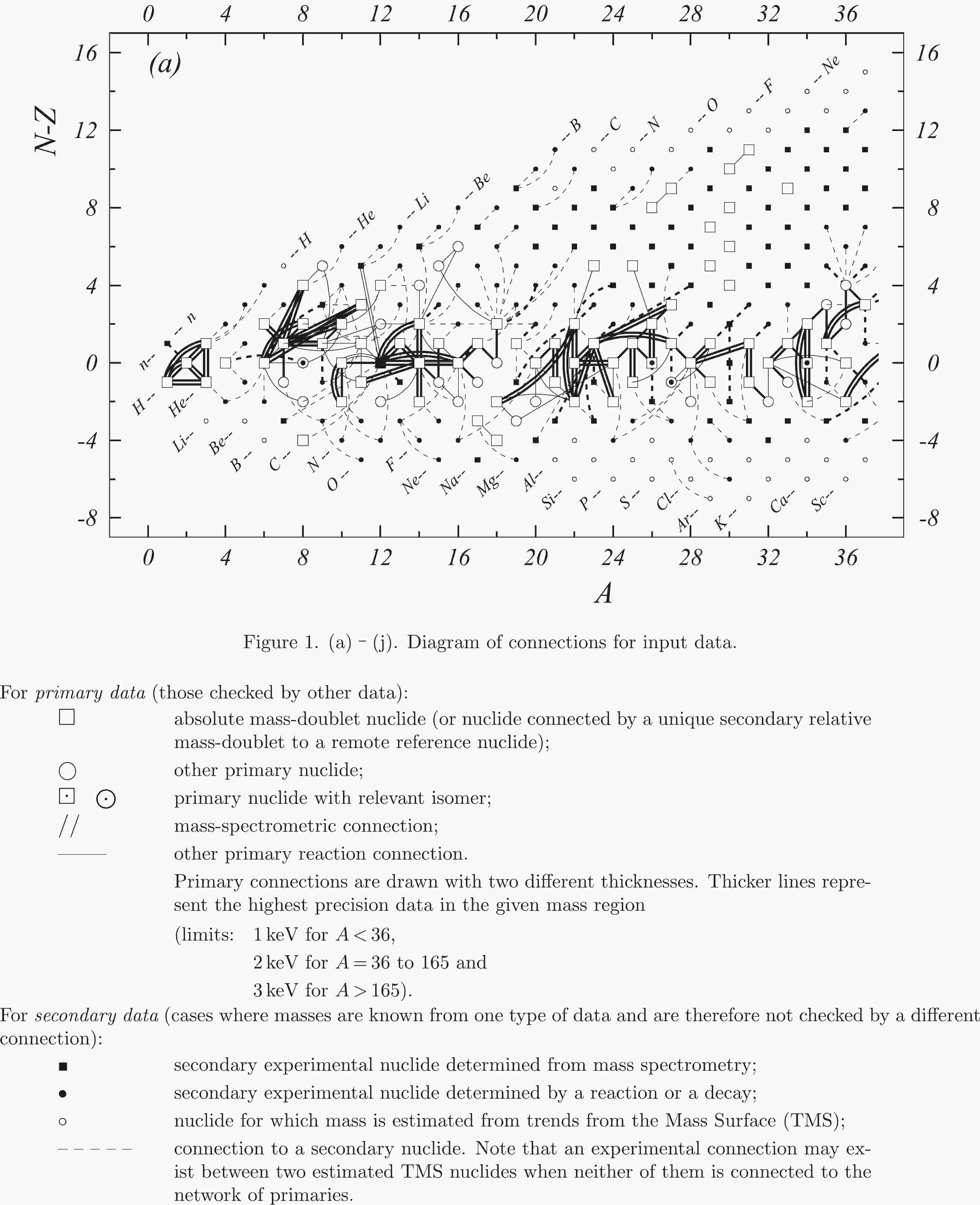
In the present work all available experimental data related to atomic masses (both energy and mass-spectrometric data) are considered. The input data are extracted from the available literature, compiled in an appropriate format and then carefully evaluated. The data are compared with other results and with values obtained from the trends from the mass surface (TMS) in the region, and the calibrations are checked, if necessary. As a consequence, some of the input data are accepted directly or after appropriate corrections and used in the subsequent mass adjustment procedure. There are also data that are not used due to large uncertainties or other reasons, as explained in section 4.5. All input data are given in Table I, and these used in the mass adjustment are also presented graphically in Fig. 1.


Figure 1b. Diagram of connections for input data — continued.
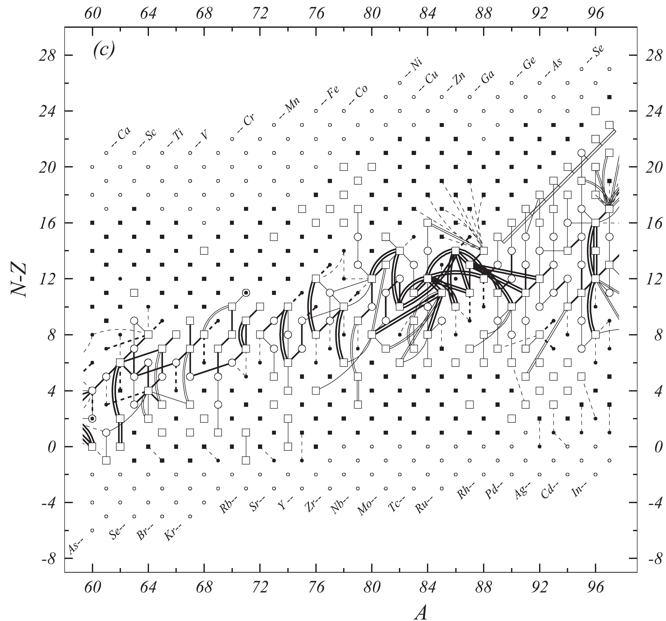
Figure 1c. Diagram of connections for input data — continued.
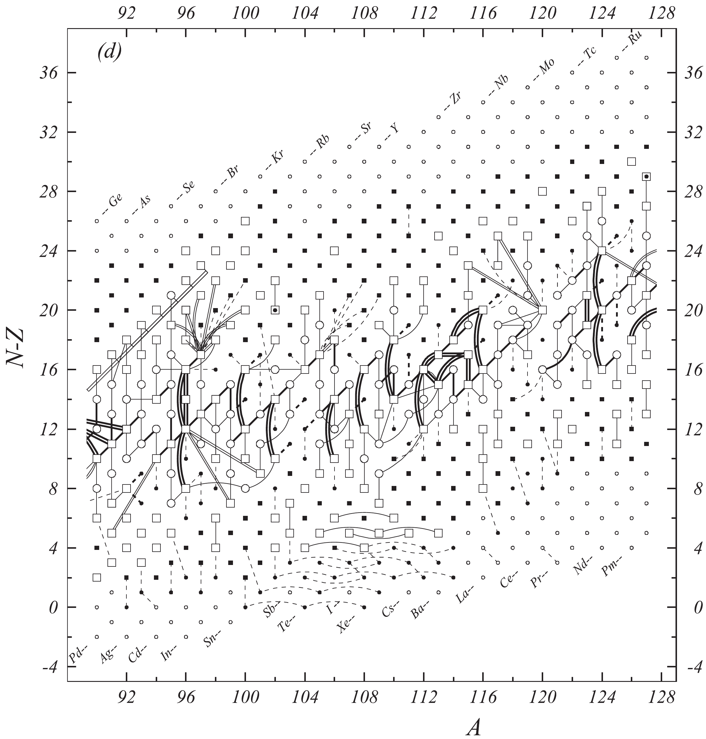
Figure 1d. Diagram of connections for input data — continued.
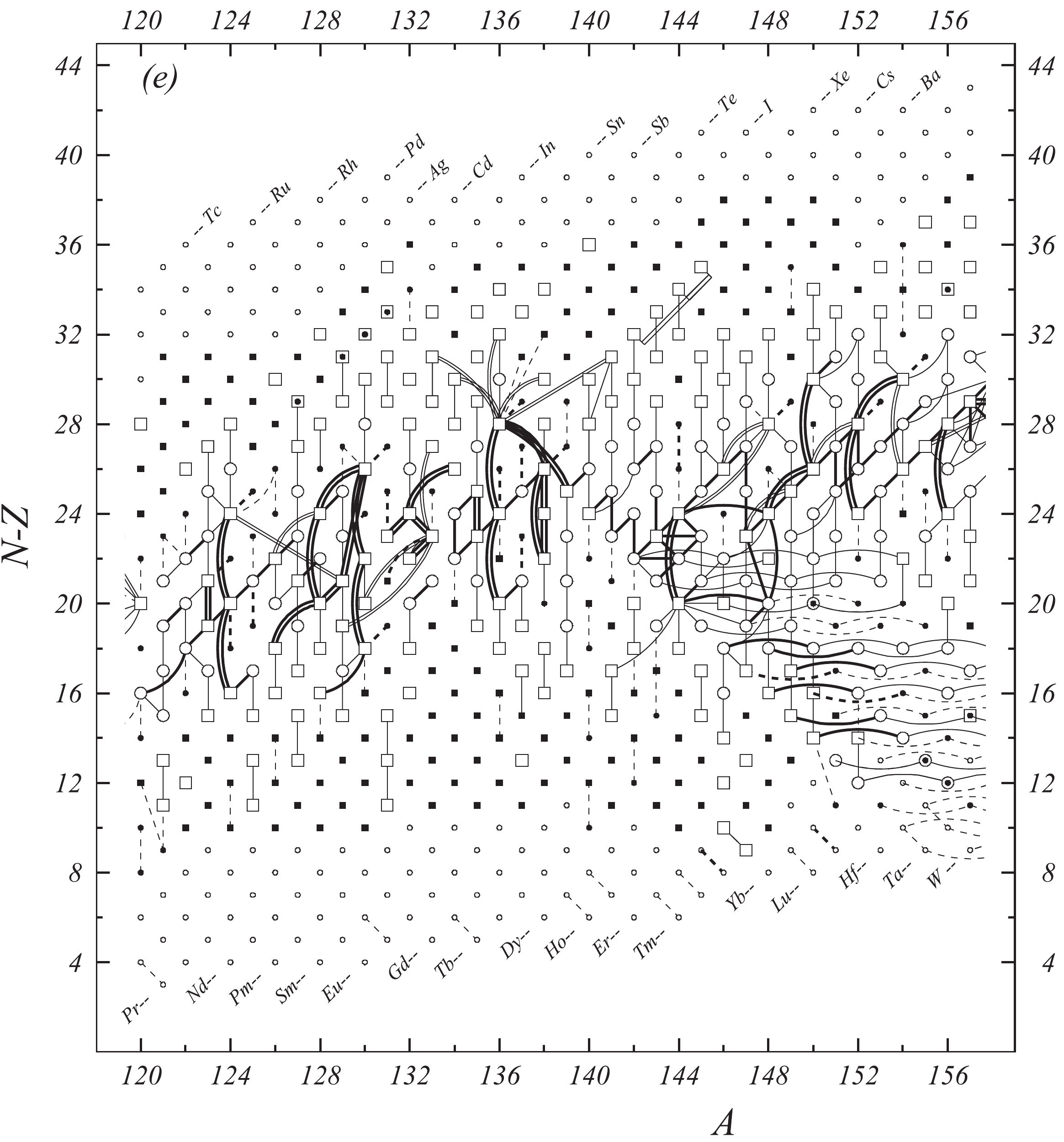
Figure 1e. Diagram of connections for input data — continued.
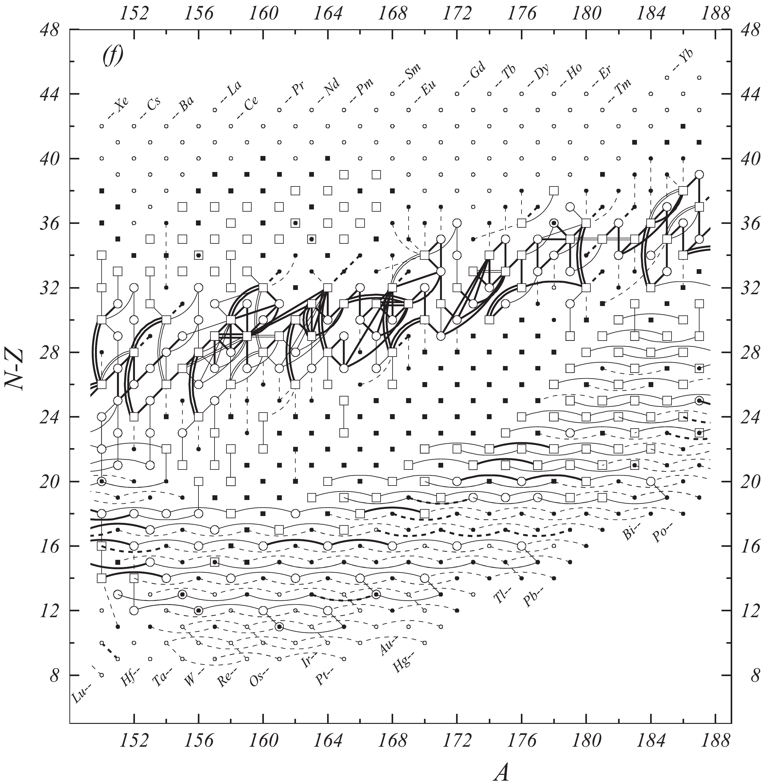
Figure 1f. Diagram of connections for input data — continued.
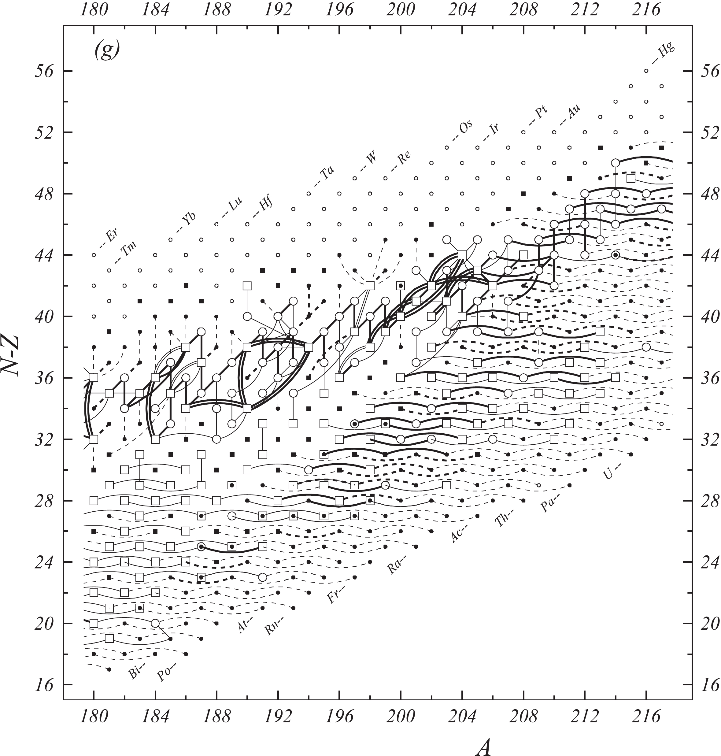
Figure 1g. Diagram of connections for input data — continued.

Figure 1h. Diagram of connections for input data — continued.
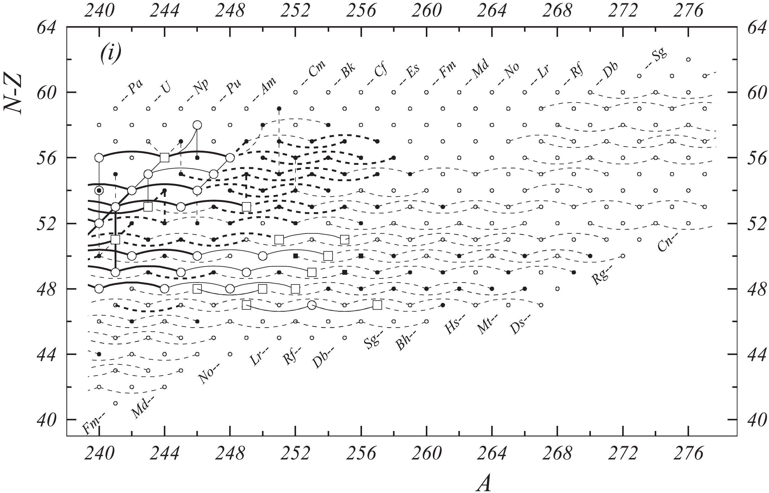
Figure 1i. Diagram of connections for input data — continued.
-
Fig. 1 shows a connection diagram of (
$ N-Z $ ) versus ($ N+Z $ ), where each dot represents a nuclide and each line connecting the dots an experimentally established relation. It is straightforward to show many mass measurements results that way, including these from mass-doublet spectroscopy or decay energy measurements. For example, mass measurements using Penning-trap almost always give a ratio of masses of two ions, as the inverse proportion to their cyclotron frequencies in the trap. Thus, in most case those measurements can be represented as a connection of two masses. For a relation of several atomic masses determined by reaction energy measurements, usually one mass difference between two nuclides is the most important one and it is then presented in the diagrams. Most lines in Fig. 1 link two nuclides, with exceptions for five mass-spectrometric "triplet" measurements of Rb and Cs isotopes from [1982Au01, 1986Au02], which can be best represented as a linear combination of three isotopes with non-integer coefficients [1982Au01].However, not all of the experimental results can be clearly represented in Fig. 1. For example, direct experimental results from 'Smith-type', 'Schottky', 'Isochronous', 'Time-of-flight' and some 'Multi-reflection Time-of-flight' mass spectrometers, are calibrated in a more complex way, and are thus published by their authors as absolute mass values. They are then shown as open squares in Fig. 1, and presented in Table I as a difference
$ ^{A} $ El—u, where$ ^{A} $ El represents the nuclide with the mass number A and element name El.Atomic masses are exacted from the network in Fig. 1. The absolute mass values in the unit 'u' can be determined experimentally for nuclides that are eventually connected to
$ ^{12} $ C, the anchor point of the network. As can be seen from Fig. 1, the accepted data may allow determination of the mass of a particular nuclide using several different routes; such a nuclide is called primary. Their mass values in the table are then derived by a least squares method. In the other cases, the mass of a nuclide can be derived from only one connection to another nuclide; it is called a secondary nuclide. This classification is of importance for our calculation procedure.The diagrams in Fig. 1 also show many cases where the relation between two atomic masses is experimentally known, but none of them are connected to
$ ^{12} $ C. Since it is our policy to include all available experimental results, in such cases we have produced estimated mass values that are based on TMS in the neighborhood. Using this data representation, vacancies also occur, and these are filled with estimated values produced by the same TMS procedure. Estimates of unknown masses are further discussed in section 5.2.Excited isomeric states may be involved in mass measurements and the related information is included in this work. Although some isomeric states are indicated in Fig. 1, the diagram itself is two-dimensional and cannot represent the experimental results involving isomers completely. Instead, all relevant information is given in Table I.
-
All input data are given as linear equations in Table I. Penning-trap mass spectrometers provide cyclotron frequencies of charged ions in the trap, which are always compared to that of a well known reference nuclide in order to determine the ratio of two masses. The mass ratios are converted to a linear combination of masses of electrically neutral atoms without any loss of accuracy. The procedure for converting frequency ratios to linear equations can be found in Appendix A. Some authors publish their results directly as masses, but this is not a recommended practice for high-precision mass measurements since the mass values could be modified due to change of the reference mass. An energy measurement of nuclear reaction or decay can be easily represented with a linear equation, too.
When it is too difficult to express a primary experimental result in a simple equation, the absolute mass value is given in Table I as a difference
$ ^{A} $ El—u and it is usually accompanied with the relevant comment to explain the original information. Such comment is not applied for results from time-of-flight mass spectrometry, where the mass of interest is obtained using complex calibrations with many reference masses and reported as an absolute mass value in the original literature.Values in the equations listed in Table I and the corresponding uncertainties are given in '
$ \mu $ u' for results from mass spectrometry and in 'keV' for energy measurements. -
A total of 777 pieces of new experimental data are included in AME2020 in comparison to AME2016. Among them, 477 data are from mass spectrometry measurements, and 300 data from energy measurements.
Updated values for the masses of
$ \pi $ $ ^{+} $ and$ \pi $ $ ^{-} $ are included from the latest Particle Data Group publication [19]. These two mesons are present since they are involved in some atomic mass experiments, although they are not considered as "nuclides" themselves. -
The most precise input data are provided by Penning traps, where the cyclotron frequencies of the ion of interest and a reference ion are measured in a uniform magnetic field. Three traps, namely LIONTRAP at Mainz, PENTATRAP at Heidelberg and FSU-MIT-TRAP at Florida, are dedicated for mass measurements of stable or long-lived nuclides with ultra-high accuracy, and provide 15 results with precisions of 0.04 nu (10
$ ^{-9} $ u) for light ions [2020Fi05], and 1.5-2.8 nu for xenon isotopes [2020Ri04]. These results provide reliable reference standards for other mass measurements.For measurements with such high precisions, not only the electronic binding energy (single or multiple ionization), but also the molecular binding energy (dissociation energy) should be considered in the data treatment. As described for example in Ref. [2018Sm03], even the rotational energy of the molecule has to be taken into account. For most molecules used in the experiments, the binding energy represents typically a correction of a few parts in
$ 10^{10} $ and its uncertainty only limits the accuracy of the neutral atomic mass to a few parts in$ 10^{12} $ . For measurements with precisions not better than$ 10^{-9} $ (100 eV/100 u), the molecular binding energy could be neglected without loss of accuracy. In cases where the precision is better than$ 10^{-10} $ (10 eV/100 u), e.g. at MIT [1995Di08] and FSU [2015My03], it is necessary to take into account the molecular binding energy. More details on the binding energy corrections can be found in Appendix A. -
The domain of nuclides with experimentally known masses has extended impressively over the last few years, thanks to the developments of radioactive nuclear beam facilities and novel mass spectrometers. Around 20 years ago, masses of short-lived nuclides were mainly known from
$ Q_\beta $ end-point measurements, while in the present evaluation, mass spectrometry dominates. It can be concluded that the shape of the atomic mass surface, and hence understanding of nuclear interactions, has been changed significantly over the last 10-20 years.In the past, several types of mass spectrometry have provided some important results for radioactive nuclides, but are not used any more. Among them, the classical double-focussing mass spectrometry and the 'Smith-type' Radio-frequency mass spectrometry MISTRAL at CERN, Cyclotron time-of-flight mass spectrometry at SARA-Grenoble and at CSS2-GANIL, were described in AME2016 and will not be discussed here. The Schottky mass spectrometry at ESR-GSI, which measures the revolution frequency of cooled nuclides in a storage ring, has not provided new data either.
All new mass-spectrometry results included in AME2020 are obtained by using one of the four methods, namely Penning traps and Multi-Reflection Time-of-Flight spectrometers (MR-TOF) for low-energy radioactive nuclides, the Magnetic-Rigidity time-of-flight (B
$ \rho $ -ToF) mass spectrometry and storage-ring based isochronous-mass-spectrometry (IMS) at high-energy facilities.Penning trap spectrometers Nowadays, seven Penning traps are being operated at major facilities for radioactive nuclide research around the world: ISOLTRAP-Cern, CPT-Argonne, JYFLTRAP-Jyväskylä, LEBIT-East-Lansing, SHIPTRAP-Darmstadt, TITAN-Vancouver, and TRIGA-TRAP-Mainz. Conventionally the Time-of-Flight Ion-Cyclotron-Resonance (ToF-ICR) method is used to determine the cyclotron frequencies of ions in the trap. High resolving power (
$ 10^6 $ ) and accuracies (to$ 10^{-8} $ ) are routinely achieved for nuclides located quite far from the line of$ \beta $ -stability. Recently, a novel method of Phase-Imaging Ion-Cyclotron-Resonance (PI-ICR) was firstly developed at SHIPTRAP using a position-sensitive detector [2013El01]. This method is more efficient and more precise than the conventional ToF-ICR. In AME2016 only SHIPTRAP reported results using PI-ICR, while in the current work ISOLTRAP, CPT and JYFLTRAP also reported such results. Thanks to the high resolving power of PI-ICR, many low-lying isomeric states can be clearly identified. For example, the isomeric state in$ ^{104} $ Nb with an excitation energy of 9.8(2.3) keV was measured by CPT [2018Or.A].Multi-Reflection Time-of-Flight spectrometers The Multi-Reflection Time-of-Flight spectrometer (MR-TOF) was initially developed for beam purification for ISOLTRAP and then used as an independent mass spectrometer. This method started to provide mass results of short-lived nuclides in 2013 and results from four MR-TOF's, operated at ISOLDE-CERN, RIBF-RIKEN, GSI and TRIUMF, are included in AME2020.
The MR-TOF mass measurements are based on time-of-flight, aiming at extending the flight path by reflecting ions back and forth in a static electric field. With this method, a relative mass precision of
$ 10^{-7} $ is routinely achieved with a typical resolution of$ 10^{-5} $ . MR-TOF spectrometer is in principle more sensitive than Penning trap and it can be used in measurements of nuclides with very short half-lives and/or low production rates. As demonstrated at ISOLDE-CERN, it can always extend the measured region by one more nuclide further away from stability compared with PENNING TRAP [2017We16, 2018Mo14, 2020Ma09].For mass determination with MR-TOF, the general relation between mass-to-charge ratio (
$ m/q $ ) and time-of-flight t is [2013Wi06]:$ t = \alpha \sqrt{m/q} + \beta , $

(1) where
$ \alpha $ and$ \beta $ are constants related to the experimental set-up and are the same for the ion of interest and for the reference ions.At RIKEN, GSI and TRIUMF, the
$ \beta $ parameter can be determined independently, thus only one reference nuclide is needed for mass calibration. In this way, the ratio of time-of-flight between the ion of interest and the reference ion is used to extract the linear equation, as it is the case for Penning trap measurement. However, at ISOLDE-CERN, two reference masses are used to determine the mass of interest, and the so-called$ C_{tof} $ method is used. When using this method, we express the linear equation in term of absolute mass.Magnetic-Rigidity Time-of-Flight spectrometers Projectile fragmentation and in-flight fission reactions are powerful tools to produce exotic nuclides far from the stability. Masses of almost undecelerated fragment products, produced in bombardment of thin targets with beams of heavy ions, can be determined from a combination of magnetic deflection and time-of-flight measurements. Nuclides in an extended region in
$ A/Z $ and Z are analyzed simultaneously. Each individual ion, even very short-lived ($ 1 \mu s $ ) one, can be identified and its mass measured. The limited resolving power of m/$ \delta $ m$ \sim10^4 $ and cross-contaminations can cause significant shifts in masses. Using this method, mass values with precisions of 3-50 ppm have been obtained for a large number of neutron-rich nuclides up to$ A\sim70 $ .One difficulty in such experiments is the presence of isomeric states with half-lives comparable or longer than the time of flight (about 1
$ \mu $ s) which may affect the mass of the ground state. In the recent work at RIKEN [2020Mi13], the isomeric ratios are also measured using$ \gamma $ -ray detectors at the experimental counting station, providing corrections for isomeric contamination. The most critical part in these experiments is the calibration, since it is frequently from an empirically determined function, which, in several cases, had to be extrapolated rather far from the calibrating masses. The MSU group re-evaluated their old B$ \rho $ -ToF experimental data [2015Me01, 2015Me08, 2016Me07], by incorporating recently published high precision Penning trap mass data [2018Le03, 2018Mo14] as additional calibration nuclides. This allowed to reduce the systematic uncertainty in previously measured data and to expand the number of nuclides for which masses were obtained [2020Me06].Isochronous Mass Spectrometry If the flight path length of the spectrometer can be extended, then the resolving power can be improved. This is the basic idea of the storage-ring based spectrometer, which has been proven to be a powerful tool for direct mass measurement of short-lived nuclides. In an Isochronous Mass Spectrometry (IMS) experiment, the revolution times of the ions stored in the storage ring are measured, from which the nuclear masses can be extracted. Since no beam cooling is needed, the IMS method is suitable to mass measurements of nuclei with half-lives as short as several microseconds. The first set-up of this type was operated at GSI-ESR at Darmstadt, but there are no new results from that group in recent years. The Cooler Storage Ring for experiment (CSRe) at the IMP-LANZHOU is the second spectrometer for IMS mass measurements. In these experiments, the drifts of the revolution times caused by instabilities of the magnetic fields are carefully corrected, and as a consequence the appropriate statistical uncertainty is assigned to each ion by evaluating the revolution times. In this way no apparent systematic uncertainty is observed, and a relative precision of 1
$ \times\; 10^{-7} $ can be routinely achieved. A new isomeric state in$ ^{101} $ In has been discovered recently, demonstrating the excellent resolving power [2019Xu13]. This result was later confirmed by MR-TOF at GSI [2020Ho03]. -
Although mass spectrometry dominates the field of high-precision mass measurements, decay energy measurements play an indispensable role in discovering new nuclides and in determining their masses.
Presently, many nuclides beyond the driplines can be accessed in the light-mass region. They can decay via direct proton or neutron emission. The half-lives of some unbound nuclides are too short to acquire their outer electrons (which takes around 10
$ ^{-14} $ s), and to form atoms. However, we still convert their masses to "atomic masses" so we can treat them consistently with other nuclides. It is challenging to experimentally study these unbound nuclides far from stability where only a very few events can be observed. Frequently, theoretical calculations are required to extract their properties from the experimental data. For example, light unbound nuclides$ ^{20} $ B and$ ^{21} $ B [2018Le18], and$ ^{31} $ K [2019Ko18] have been discovered using complete kinematic measurement of all decay products, and their masses determined with the invariant mass spectrum. Another example is the mass of$ ^{73} $ Rb which was determined in$ \beta $ -delayed proton measurement [2020Ho17].Of the 300 newly included energy results in AME2020, 237 are
$ \alpha $ decay energy measurements. Fusion reactions are frequently used for the synthesis of new neutron-deficient nuclides in the medium and heavy mass regions. Several new neutron-deficient uranium and neptunium isotopes were discovered using this approach in Lanzhou. The nuclides were identified by the characteristic$ \alpha $ decays along the decay chains, and their masses are deduced from the measured$ \alpha $ -decay energies [2019Zh23, 2020Ma09]. -
In most cases, values given by authors in the original publication are accepted by the AME evaluators, but there are exceptions. One example is the performed recalibration due to the change in the definition of volt, as discussed in Section 2. For more complex cases, a remark is added in Table I at the end of the concerned A-group.
Changes in the uncertainties of the
$ \alpha $ -decay energies are also introduced, when it is not clear if the final state is the ground state or an excited one. For these cases, an extra 50 keV is added in quadrature to the original uncertainty. -
The resolving power of mass spectrometers improved significantly in recent years and many isomers can be clearly identified and their masses unambiguously measured. However, there are cases where a mixture of isomers is actually measured. Since the mass of the ground state is the primary aim of the present evaluation, it can be derived only in cases where information on the excitation energies and production rates of the isomers is available. In AME, we use a special treatment of isomer mixtures (see Appendix B) and information about such changes is given as comments to the input data in Table I.
The mass
$ M_0 $ of the ground state can be calculated if both the excitation energy$ E_1 $ of the upper isomer and its relative production rates are known, as discussed in [2020Ca08]. However, such detailed information is usually lacking in the literature. In such cases, if$ E_1 $ is known but not the production ratio, one must assume equal probabilities for all possible relative intensities. The estimated mass of the ground state is then$ M_0 $ =$ M_{exp}-E_1/2 $ , and the uncertainty is 0.29$ E_1 $ (see Appendix B). For cases where two or more excited isomers are involved, the correction method is discussed in Appendix B.A further complication arises when
$ E_1 $ is not known. In such a case, we use an estimate value for E1, flagged with '#', which is incorporated in the NUBASE evaluation. When estimating the$ E_1 $ values, we first consider the available experimental data possibly giving lower limits: e.g. if it is known that one of two isomers decays to the other; or if$ \gamma $ rays of known energy occur in such decays. If not, we try to interpolate between$ E_1 $ values in neighboring nuclides that can be expected to have the same spin and configuration assignments. If such a comparison does not yield useful results, theoretical predictions were sometimes accepted, including upper limits for transition energies following from the measured half-lives. Values estimated this way are provided with somewhat generous uncertainties.In general, an isomer can affect the mass of the ground state if its lifetime is relatively long (hundreds of milliseconds or longer). However, half-life values given in NUBASE are those for neutral atoms. For bare nuclides, where all electrons are fully stripped from the atom, the lifetimes of such isomers can be considerably longer, since the decay by conversion electrons is switched off. One example is the half-life measurement of the fully-stripped
$ ^{94m} $ Ru$ ^{44+} $ by means of IMS at CSRe [2017Ze02]. -
Sometimes, conflicting meanings of particle and decay energies are given in the literature. For example, energy values are given by some authors as the particle energy E, while others quote it as decay energy Q, which is the sum of kinetic energies of the emitted particle and the recoiling daughter nuclide. In general, the
$ \alpha $ particle carries about 97-98% of its Q value and the recoiling nuclide accounts for about 2-3%. The relation between the$ Q_{\alpha} $ and$ E_{\alpha} $ values is discussed in Appendix C.Some authors derive
$ Q_{\alpha} $ value by not only correcting for the recoil energy, but also for the effect of screening by the atomic electrons (see Appendix C). In our adjustment procedure, the latter corrections have been removed.Recalibration of decay energies in implantation experiments In experiments where
$ \alpha $ - and proton-emitting nuclei are implanted in a silicon detector, both the$ \alpha $ particle and the recoiling daughter nuclide deposit energies in the detector. In such cases,$ \alpha $ particles and protons with energies of a few MeV have almost 100% detection efficiency, which is not the case for the heavy recoiling nuclides, where only part of the recoiling energy contributes to the signal.This effect has been discussed in Ref. [2012Ho12] and the partial recoil energy of the daughter nuclide has been taken into account in the energy calibration. However, not all authors make such corrections to their published data. We have developed a procedure [20] to calculate the detection efficiency for heavy nuclides in silicon detectors based on the Lindhard's theory [21], which has been experimentally proven to be reliable [22,23].
The correction has been applied only to a few experimental results in the present work and a remark is added in Table I. After discussions with the authors of the original publication, the
$ \alpha $ -decay energy of$ ^{255m} $ Lr from Ref. [2008Ha31] has been corrected and the difference turns out to be 7 keV. Another example is the proton-decay energy of$ ^{53m} $ Co from [2015Sh16], as discussed in Ref. [20]. -
The atomic mass evaluation is unique when compared to the other evaluations of data, in the sense that all mass determinations are relative measurements, not absolute ones. Each experimental datum defines a relation involving two or more nuclides. The ensemble of these relations generates a highly entangled network, as represented in Fig. 1. All the input data are given as linear equations in Table I.
To determine the mass values, we use a least-squares method weighed according to the uncertainty with which each piece of data is known. In the first step, we pre-average the same and parallel data to reduce the size of the system of equations, and then separate primary data from secondary ones. The primary data are used in the following least-squares calculations. At last, we recommend the atomic masses (Part II, Table I), the nuclear reaction and separation energies (Part II, Table III), the adjusted values for the input data (Table I), the influences of data on the primary nuclides (Table I), the influences received by each primary nuclide (Part II, Table II), and display information on the inversion errors, the correlations coefficients (Part II, Table B), the
$ \chi^2 $ values, the distribution of the$ v_i $ (see below), among others. -
Two or more measurements of the same physical quantities can be replaced without loss of information by their average value and precision, reducing thus the system of equations to be treated. By extending this procedure, we consider parallel data: reaction data occur that give values essentially for the mass difference of the same two nuclides, except in rare cases where the precision is comparable to that in the masses of the reaction particles. Example:
$ ^{14} $ C($ ^7 $ Li,$ ^7 $ Be)$ ^{14} $ B and$ ^{14} $ C($ ^{14} $ C,$ ^{14} $ N)$ ^{14} $ B; or$ ^{22} $ Ne(t,$ ^3 $ He)$ ^{22} $ F and$ ^{22} $ Ne($ ^7 $ Li,$ ^7 $ Be)$ ^{22} $ F. For this kind of case, one of the two links is replaced by an equivalent value for the other, and the pre-averaging procedure works as for the same quantities.If the Q data to be pre-averaged are strongly conflicting, i.e. if the consistency factor (or Birge ratio)
$ \chi_n = \sqrt{\chi^2/(Q-1)} $ resulting in the calculation of the pre-average is greater than 2.5, the (internal) precision$ \sigma_i $ in the average is multiplied by the Birge ratio ($ \sigma_e = \sigma_i \chi_n $ ). The quantity$ \sigma_e $ is often called the ‘external error’. Un-weighted average is also used in some cases, where the corresponding remarks are given in Table I. The pre-averaged data with largest discrepancies are listed in Table C. Most of these have already been displayed in the similar table in AME2016 [2]. Only one new item, namely$ ^{12} $ O(2p)$ ^{10} $ C, is added in the current table due to the new input data. Six items shown in AME2016 are now removed and instead listed in Table D, where the resolution of the discrepancies is given.Item n $ \chi_n $ 

$ \sigma_e $ 

Item n $ \chi_n $ 

$ \sigma_e $ 

$ ^{186} $ W(n,

$ \gamma $ )

$ ^{187} $ W

2 2.44 0.11 $ ^{177} $ Pt(

$ \alpha $ )

$ ^{173} $ Os

2 2.06 6.06 $ ^{144} $ Ce(

$ \beta^- $ )

$ ^{144} $ Pr

2 2.44 2.18 $ ^{244} $ Cf(

$ \alpha $ )

$ ^{240} $ Cm

2 2.03 3.97 $ ^{220} $ Fr(

$ \alpha $ )

$ ^{216} $ At

2 2.34 4.66 $ ^{15} $ N(p,n)

$ ^{15} $ O

2 2.03 1.28 $ ^{75} $ As(n,

$ \gamma $ )

$ ^{76} $ As

2 2.32 0.17 $ ^{58} $ Fe(t,p)

$ ^{60} $ Fe

4 2.03 7.38 $ ^{110} $ In(

$ \beta^+ $ )

$ ^{110} $ Cd

3 2.29 28.4 $ ^{204} $ Tl(

$ \beta^- $ )

$ ^{204} $ Pb

2 2.03 0.39 $ ^{40} $ Cl(

$ \beta^- $ )

$ ^{40} $ Ar

2 2.21 76.1 $ ^{106} $ Ag(

$ \varepsilon $ )

$ ^{106} $ Pd

2 1.98 6.63 $ ^{153} $ Gd(n,

$ \gamma $ )

$ ^{154} $ Gd

2 2.16 0.39 $ ^{78} $ Se(n,

$ \gamma $ )

$ ^{79} $ Se

3 1.96 0.28 $ ^{113} $ Cs(p)

$ ^{112} $ Xe

3 2.10 5.03 $ ^{46} $ Ca(n,

$ \gamma $ )

$ ^{47} $ Ca

2 1.94 0.56 $ ^{27} $ P

$ ^i $ (2p)

$ ^{25} $ Al

2 2.08 74.7 $ ^{181} $ Pb(

$ \alpha $ )

$ ^{177} $ Hg

3 1.93 15.2 $ ^{12} $ O(2p)

$ ^{10} $ C

2 2.08 26.8 $ ^{145} $ Sm(

$ \varepsilon $ )

$ ^{145} $ Pm

2 1.92 7.92 $ ^{204} $ Rn—

$ ^{208} $ Pb

$ _{0.981} $ 

2 2.06 18.2 $ ^{234} $ Th(

$ \beta^- $ )

$ ^{234} $ Pa

$ ^m $ 

3 1.90 2.10 Table C. Worst pre-averagings. n is the number of data in the pre-average.
Item $n$ 

$\chi_n$ 

$\sigma_e$ 

solution $^{146}$ Ba(

$\beta^-$ )

$^{146}$ La

2 2.24 107.4 new data available for $^{146}$ Ba

$^{219}$ U(

$\alpha$ )

$^{215}$ Th

2 2.18 38.5 new data available $^{36}$ S(

$^{11}$ B,

$^{13}$ N)

$^{34}$ Si

3 2.14 32.4 new data available for $^{34}$ Si

$^{223}$ Pa(

$\alpha$ )

$^{219}$ Ac

2 2.09 10.0 uncertainty increased for ambiguous transition $^{278}$ Mt(

$\alpha$ )

$^{274}$ Bh

3 1.98 43.6 uncertainty increased for ambiguous transition $^{167}$ Os(

$\alpha$ )

$^{163}$ W

4 1.98 3.50 uncertainty increased for ambiguous transition Table D. Worst pre-averagings shown in AME2016 and removed in the current work, together with the solutions
In the present evaluation, we have replaced 2980 data by 1189 averages. As much as 21.8% of which have values of
$ \chi_n $ (Birge ratio) beyond unity, 1.34% beyond two and none beyond 3, giving an overall very satisfactory distribution for our treatment. As a matter of fact, in a complex system like the one here, many values of$ \chi_n $ beyond 1 or 2 are expected to exist, and if the uncertainties were multiplied by$ \chi_n $ in all these cases, the$ \chi^2 $ -test on the total adjustment would have been invalidated. This explains the choice we made here of a rather high threshold ($ \chi_n^0 = 2.5 $ ), compared e.g. to$ \chi_n^0 = 1 $ used in a different context by the Particle Data Group [19], for departing from the rule of 'internal error' of the weighted average.Besides the computer-automated pre-averaging, we found it convenient, in some
$ \beta^+ $ -decay cases, to combine results stemming from various capture ratios in an average. These cases are$ ^{109} $ Cd($ \varepsilon $ )$ ^{109} $ Ag (average of 3 data),$ ^{139} $ Ce($ \varepsilon $ )$ ^{139} $ La (average of 10) and$ ^{195} $ Au($ \varepsilon $ )$ ^{195} $ Pt (5 results), and they are detailed in Table I. Four more cases ($ ^{147} $ Tb,$ ^{152} $ Ho,$ ^{166} $ Yb and$ ^{207} $ Bi) occur in our list, but they carry no weight and are labeled with 'U' in Table I. -
In averaging
$ \beta $ - ($ \alpha $ -) decay energies derived from branches observed in the same experiment, to or from different levels in the decay of a given nuclide, the uncertainty we use for further evaluation is not the one resulting from the weighted average adjustment, but instead we use the smallest experimental one. In this way, we avoid decreasing artificially the part of the uncertainty that is not due to statistics. In some cases, however, when it is obvious that the uncertainty is dominated by weak statistics, we do not follow the above rule (e.g.$ ^{23} $ Al$ ^i $ (p)$ ^{22} $ Mg of [1997Bl04]).Some quantities have been reported more than once by the same group. If the results are obtained by the same method in different experiments and are published in regular refereed journals, usually only the most recent one is used in the calculation. There are two reasons for this policy. The first is that one might expect that the authors, who believe their two results are of the same quality, would have averaged them in their latest publication. The second is that if we accept and average the two results, we would have no control on the part of the uncertainty that is not due to statistics. Our policy is different when the newer result is published in a secondary reference (not refereed abstract, preprint, private communication, conference, thesis or annual report). In such cases, the older result is used in the calculations, except when the newer one is an update of the previous value. In some case, when the systematic uncertainties are discussed explicitly, all the independent results are used.
-
Another feature to increase the meaning of the final
$ \chi^2 $ in the least-squares procedure, is to not use data with weights at least a factor 10 smaller than the combination of all other data giving the same result. Such data were labeled with 'U' in the list of input data; comparison with the output values allows to check our judgment. Until the AME2003 evaluation, our policy was not to print data labeled 'U' if they already appeared in one of our previous tables, reducing thus the size of the table of data to be printed. This policy has been changed since AME2012 [24,25], and we try as much as possible to give all relevant data, also including insignificant ones. The reason for this is that conflicts might appear amongst recent results, and access to older ones might shed some light on evaluating the new data. -
In Section 3, while examining the diagrams of connections (Fig. 1), we noticed that, whereas the masses of secondary nuclides can be determined uniquely from the chain of secondary connections going down to a primary nuclide, only the latter see the complex entanglement that necessitated the use of the least-squares method.
In terms of equations and parameters, we consider that if, in a collection of equations to be treated with the least-squares method, a parameter occurs in only one equation, removing this equation and this parameter will not affect the result of the fit for all other data. Thus, we can redefine more precisely what was called secondary in Section 3: the parameter above is a secondary parameter (or mass) and its related equation is a secondary equation. After the reduced set has been solved, then the secondary equation can be used to determine the final value and uncertainty for that particular secondary parameter. The equations and parameters remaining after taking out all secondaries are called primary.
Therefore, only the system of primary data is overdetermined, and thus will be improved in the adjustment, so that each primary nuclide will benefit from all the available information. Secondary data will remain unchanged; they do not contribute to
$ \chi^2 $ . The diagrams in Fig. 1 show, that many secondary data exist. Thus, taking them out simplifies considerably the system. More importantly, if a better value is found for a secondary datum, the mass of the secondary nuclide can easily be improved. The procedure is more complicated for new primary data.We define DEGREES for secondary nuclides and secondary data. They reflect their distances along the chains connecting them to the network of primaries. The first secondary nuclide connected to a primary one will be a nuclide of degree 2; and the connecting datum will be a datum of degree 2 as well. Degree 1 is for primary nuclides and data. Degrees for secondary nuclides and data range from 2 to 17. It is the nuclide
$ ^{291} $ Lv that has the highest degree number 17. Its mass is determined through a long$ \alpha $ chain, although many of them are just estimates. In Table I, the degree of data is indicated in column 'Dg'. In the table of atomic masses (Part II, Table I), each secondary nuclide is marked with a label in column 'Orig.' indicating from which other nuclide its mass value is determined. The word primary used for these nuclides and for the data connecting them does not mean that they are more important than the others, but only that they are subject to the least-squares treatment above. The labels primary and secondary are not intrinsic properties of data or nuclides. They may change from primary to secondary or vice versa when other information becomes available.To summarize, separating secondary nuclides and secondary data from primaries significantly reduces the size of the system that will be treated by the least-squares method, and allows better insight into the relations between data and masses. After treatment of the primary data alone, the adjusted masses for primary nuclides can be easily combined with the secondary data to yield masses of secondary nuclides.
-
Each piece of data has a value
$ q_i \pm dq_i $ with the accuracy$ dq_i $ (one standard deviation) and makes a relation between two, three or four masses with unknown values$ m_{\mu} $ . An overdetermined system of Q data to M masses ($ Q > M $ ) can be represented by a system of Q linear equations with M parameters:$ \sum\limits_{\mu = 1}^M k_i^{\mu} m_{\mu} = q_i \pm dq_i , $

(2) e.g. for a nuclear reaction
$ A(a,b)B $ requiring an energy$ q_i $ to occur, the energy balance is written:$ m_{\rm A} + m_{\rm a} - m_{\rm b} - m_{\rm B} = q_i \pm dq_i . $

(3) Thus,
$ k_i^{\rm A} = +1 $ ,$ k_i^{\rm a} = +1 $ ,$ k_i^{\rm b} = -1 $ and$ k_i^{\rm B} = -1 $ .In matrix notation,
$ {\bf K} $ being the$ (Q,M) $ matrix of coefficients, Eq. 2 is written:$ {\bf K} \vert m\rangle = \vert q\rangle $ . Elements of matrix$ {\bf K} $ are almost all null: e.g. for$ A(a,b)B $ , Eq. 3 yields a line of$ {\bf K} $ with only four non-zero elements.We define the diagonal weight matrix
$ {\bf W} $ by its elements$ w_i^i = 1 / (dq_idq_i) $ . The solution of the least-squares method leads to a very simple construction:$ {\bf ^tKWK} \vert m\rangle = {\bf ^tKW} \vert q\rangle . $

(4) The NORMAL matrix
$ {\bf A} = {\bf ^tKWK} $ is a square matrix of order M, positive-definite, symmetric and regular and hence invertible [26]. Thus the vector$ \vert\overline m\rangle $ for the adjusted masses is:$ \vert \overline m\rangle = {\bf {A^{-1}} \; ^tKW} \vert q\rangle \;\;\;{\rm or}\;\;\; \vert \overline m\rangle = {\bf R} \vert q\rangle . $

(5) The rectangular
$ (M,Q) $ matrix$ {\bf R} $ is called the RESPONSE matrix.The diagonal elements of
$ {\bf A^{-1}} $ are the squared errors on the adjusted masses, and the non-diagonal ones$ (a^{-1})_{\mu}^{\nu} $ are the coefficients for the correlations between masses$ m_{\mu} $ and$ m_{\nu} $ . Values for correlation coefficients for the most precise nuclides are given in Table B of Part II. Starting from AME2012 [24,25], we now give on the website of the AMDC [27] the full list of correlation coefficients, allowing any user to perform exact calculation of any combination of masses.One of the most powerful tools in the least-squares calculation described above is the flow-of-information matrix, discovered in 1984 [28]. This matrix allows to trace back the contribution of each individual piece of datum to each of the parameters (here the atomic masses). The AME uses this method since 1993.
The flow-of-information matrix
$ {\bf F} $ is defined as follows:$ {\bf K} $ , the matrix of coefficients, is a rectangular$ (Q,M) $ matrix. The transpose of the response matrix$ {\bf ^tR} $ is also a$ (Q,M) $ rectangular one. The$ (i,\mu) $ element of$ {\bf F} $ is defined as the product of the corresponding elements of$ {\bf ^tR} $ and of$ {\bf K} $ . In Ref. [28], it is demonstrated that such an element represents the "influence" of datum i on parameter (mass)$ m_{\mu} $ . A column of$ {\bf F} $ thus represents all the contributions brought by all data to a given mass$ m_{\mu} $ , and a line of$ {\bf F} $ represents all the influences given by a single piece of data. The sum of influences along a line is the "significance" of that datum. It has also been proven [28] that the influences and significances have all the expected properties, namely that the sum of all the influences on a given mass (along a column) is unity, that the significance of a datum is always less than unity and that it always decreases when new data are added. The significance defined in this way is exactly the quantity obtained by squaring the ratio of the uncertainty on the adjusted value over that of the input one, which was the recipe used before the discovery of the$ {\bf F} $ matrix to calculate the relative importance of data.A simple interpretation of influences and significances can be obtained in calculating, from the adjusted masses and Eq. 2, the adjusted data:
$ \vert \overline q\rangle = {\bf KR} \vert q\rangle. $

(6) The
$ i^{th} $ diagonal element of$ {\bf KR} $ represents then the contribution of datum i to the determination of$ \overline{q_i} $ (same datum): this quantity is exactly what is called above the significance of datum i. This$ i^{th} $ diagonal element of$ {\bf KR} $ is the sum of the products of line i of$ {\bf K} $ and column i of$ {\bf R} $ . The individual terms in this sum are precisely the influences defined above.The flow-of-information matrix
$ {\bf F} $ , provides thus insight on how the information from datum i flows into each of the masses$ m_{\mu} $ .The flow-of-information matrix cannot be given in full in a printed table. It can be observed along lines, displaying for each datum, the nuclides influenced by this datum and the values of these influences. It can be observed also along columns to display for each primary mass all contributing data with their influence on that mass.
The first display is partly given in the table of input data (Table I) in column 'Signf.' for the significance of primary data and 'Main infl.' for the largest influence. Since in the large majority of cases only two nuclides are concerned in each piece of data, the second largest influence could easily be deduced. It is therefore not felt necessary to give a table of all influences for each primary datum.
The second display is given in Part II, Table II for the up to three most important data with their influence in the determination of each primary mass.
-
The system of equations being largely over-determined (
$ Q>>M $ ) offers the evaluator several interesting possibilities to examine and judge the data. One might for example examine all data for which the adjusted values deviate significantly from the input ones. This helps to locate erroneous pieces of information. One could also examine a group of data in one experiment and check if the uncertainties assigned to them in the experimental paper were not underestimated.If the precisions
$ dq_i $ assigned to the data$ q_i $ were indeed all accurate, the normalized deviations$ v_i $ between adjusted$ \overline q_i $ (Eq. 6) and input$ q_i $ data,$ v_i = (\overline q_i - q_i)/dq_i $ , would be distributed as a Gaussian function of standard deviation$ \sigma = 1 $ , and would make$ \chi^2 $ :$ \chi^2 = \sum\limits_{i = 1}^Q \left(\frac{\overline q_i - q_i}{dq_i}\right)^2 \quad {\rm or}\quad \chi^2 = \sum\limits_{i = 1}^Q v_i^2 $

(7) equal to
$ Q-M $ , the number of degrees of freedom, with a standard deviation of$ \sqrt{2(Q-M)} $ .One can define as above the NORMALIZED CHI,
$ \chi_n $ (or 'consistency factor' or 'Birge ratio'):$ \chi_n = \sqrt{\chi^2/(Q-M)} $ for which the expected value is$ 1\pm1/\sqrt{2(Q-M)} $ .Another quantity of interest for the evaluator is the PARTIAL CONSISTENCY FACTOR,
$ \chi_n^p $ , defined for a (homogeneous) group of p data as:$ \chi_n^p = \sqrt{\frac{Q}{Q-M} \phantom{0} \frac{1}{p} \phantom{0} \sum\limits_{i = 1}^p v_i^2} . $

(8) The
$ \chi_n^p $ reduces to$ \chi_n $ if the sum is taken over all the input data.One can consider groups of data related to a given laboratory and with a given method of measurement and examine the
$ \chi_n^p $ of each of them. Since various methods are used in mass determination, possible systematic errors associated with a specific method, that are beyond control in experiments and not accounted for in the reported uncertainties, can be observed by the mass evaluators when considering the mass adjustment as a whole. There are presently 278 groups of data in Table I (among which 185 have at least one measurement used in determining the masses), identified in column 'Lab'. A high value of$ \chi_n^p $ might be a warning on the validity of the considered group of data within the reported uncertainties. We used such analyses to locate questionable groups of data. Each group of mass-spectrometric data is assigned a factor F according to its partial consistency factor$ \chi_n^p $ , due to the fact that its statistical uncertainties and its internal systematic error alone do not reflect the real experimental situation. From comparison to all other data and more specially to combination of reaction and decay energy measurements, we have assigned factors F of 1.5, 2.5 or 4.0 to the different labs. Example: the group of data H25 has been assigned$ F = 2.5 $ , this means that the total uncertainty assigned to$ ^{155} $ Gd$ ^{35} $ Cl$ -^{153} $ Eu$ ^{37} $ Cl is$ 2.5\times $ 2.4$ \mu $ u. The weight of this piece of data is then very low, compared to 0.79$ \mu $ u derived from all other data. This is why it is labeled "U".As in our previous works, we have estimated the average accuracy for 185 groups of data used in the evaluation that were related to a given laboratory and a specific method of measurement, by calculating their partial consistency factors
$ \chi_n^p $ . As much as 98 groups have$ \chi_n^p $ larger than unity, and 2 groups larger than 2. -
The important interdependence of most data, as illustrated by the connection diagrams (Figs. 1a—1j), allows local and global consistency tests. These can indicate that something may be wrong with the input values. We follow the policy of checking all significant data that differ by more than two (sometimes 1.5) standard deviations from the adjusted values. Fairly often, examination of the experimental results shows that a correction is necessary. Possible reasons could be that a particular decay has been assigned to a wrong final level or that a reported decay energy belongs to an isomer, rather than to a ground state, or even that the mass number assigned to a decay was incorrect. In such cases, the values are corrected and remarks are added below the corresponding A-group of data in Table I, in order to explain the reasons for the corrections.
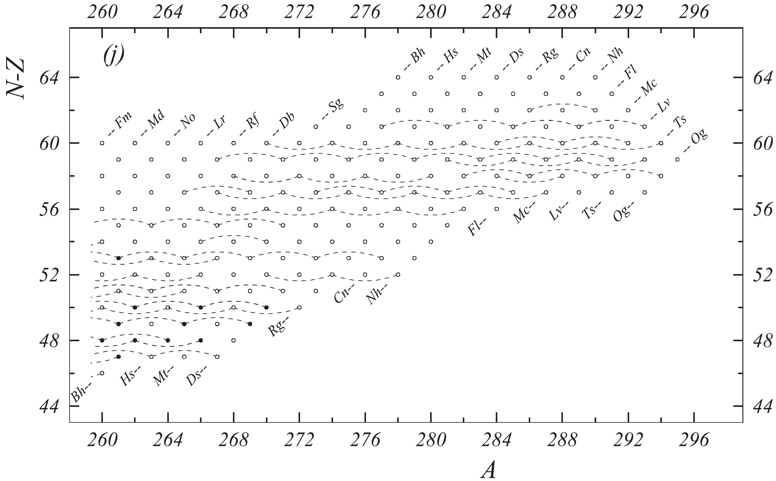
Figure 1j. Diagram of connections for input data — continued.
It also happens that a careful examination of a particular paper would lead to serious doubts about the validity of the results within the reported precision, but could not permit making a specific correction. Doubts can also be expressed by the authors themselves. The results are given in Table I and compared with the adjusted values. They are labeled 'F', and not used in the final adjustment, but always followed by a comment to explain the reason for this label. The reader may observe that in several cases the difference between the experimental and adjusted values is small compared to the experimental uncertainty: this does not disprove the correctness of the label 'F' assignment.
It happens quite often that two (or more) pieces of data are discrepant, leading to important contribution to the
$ \chi^2 $ . A detailed examination of the papers may not allow correction or rejection, indicating that at least the results in one of them could not be trusted within the given uncertainties. Then, based on past experience, we use in the calculations the value that seems to be the most reliable, while the other is labeled 'B', if published in a regular refereed journal, or 'C' otherwise.In some cases, detailed analysis of strongly conflicting data could not lead to reasons to assume that one of them is more dependable than the others or could not lead to a rejection of a particular data entry. Also, bad agreement with other data is not the only reason to doubt the correctness of the reported data. As in previous AME, and as explained above (see Section 4), we made use of the property of regularity of the surface of masses in making a choice, as well as in further checks on the other data.
When one mass is only determined by one single experimental result, but the result is strongly doubted, the policy defined for 'irregular masses' with 'D'-label assignment may apply and discussed in section 5.1.
We do not accept experimental results if information on other quantities (e.g. half-lives), derived in the same experiment and for the same nuclide, were in strong contradiction with well established values.
Data with labels 'F', 'B', 'C' or 'D' are not used in the calculations. The least-squares calculations are then done in iterations. This recipe is unavoidably subjective, but has proven to be efficient through the agreement of these estimates with newly measured masses in a great majority of cases.
-
In this evaluation, we have 13812 experimental data of which 6023 are labeled 'U' (see above), 997 are labeled 'O' (old result from same group) and 951 are not accepted and labeled 'B', 'C', 'D' or 'F' (respectively 533,161, 81 and 176 items). In the calculation we have thus 5841 valid input data, compressed to 4050 in the pre-averaging procedure. Separating secondary data, leaves a system of 2201 primary data, representing 1135 primary reactions and decays, and 1066 primary mass-spectrometric measurements. These primary data are used to determine 1304 primary masses (
$ ^{12} $ C not included). Thus, we have to solve a system of 2201 equations with 1304 parameters. Theoretically, the expectation value for$ \chi^2 $ should be 897$ \pm $ 42 (and the theoretical$ \chi_n = 1\pm0.024 $ ). The total$ \chi^2 $ of the adjustment is actually 938 ($ \chi_n = 1.023 $ ), thus showing that the ensemble of evaluated data was of good quality, and that the adopted criteria of selection and rejection of input data were adequate.In the present AME, there are 2550 masses for ground state and 406 masses for excited isomers derived from experimental results. Among the 2550 experimental ground state masses, 122 nuclides have a precision better than 0.1 keV, 402 better than 1 keV, 1532 better than 10 keV, 2407 better than 100 keV (respectively 107,366, 1499 and 2340 in AME2016). There are 143 nuclides known with uncertainties larger than or equal to 100 keV (158 in AME2016).
The mass precision has been improved for 427 nuclides in comparison with AME2016, as illustrated in Fig. 2, where the ratios of their mass uncertainties in AME2016 and AME2020 are displayed in a color code. Meanwhile, masses of 74 nuclides, which were unknown experimentally in AME2016, are measured and provided in the current mass table, as shown with black squares in Fig. 2.
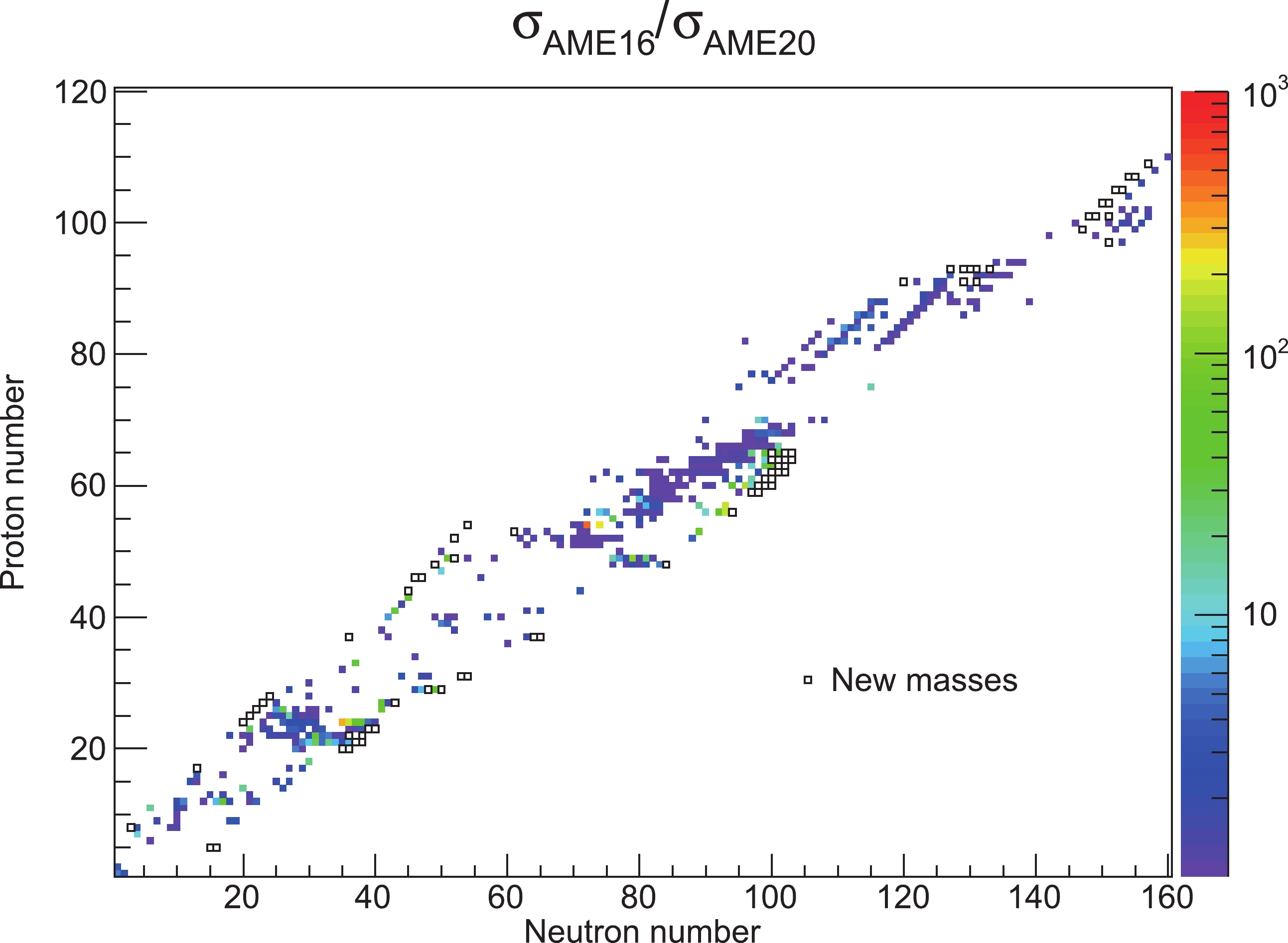
Figure 2. Ratios of mass uncertainties in AME2016 and AME2020 for nuclides whose mass precisions have been improved. The new experimental masses in AME2020 are shown as the black squares.
-
We recommend the estimated mass values for some nuclides whose mass is not determined experimentally as well as for nuclides where the experimental value is seriously questioned. The values are estimated based on the trends from the mass surface (TMS), with the assumption that the mass surface is generally smooth. An interactive graphical program is used [29] that allows a simultaneous observation of four graphs, either for the particle energies or for the differences compared with a mass model, as a function of any of the variables N, Z, A,
$ N-Z $ or$ N-2Z $ , while drawing iso-lines (lines connecting nuclides having same parameter) of any of these quantities. The mass of a nuclide can be modified or created in any view and we can determine how much freedom is left in setting a value for this mass. At the same time, interdependence through secondary connections are taken into account. In cases where two tendencies may alternate, following the parity of the proton or of the neutron numbers, one of the parities may be deselected.The replaced values for data yielding the ‘irregular masses' as well as the 'estimated unknown masses’ (see below) are thus derived by observing the continuity property in several views of the mass surface, with all the consequences due to connections to masses in the same chain. The estimated values are also compared with the predictions of available mass models. All values not derived from experimental data alone, have been clearly marked with the hashmark '#' symbol in all tables, here and in Part II. Since publication of AME1983 [30], the uncertainties are also given for the estimated data derived from TMS. These uncertainties are obtained by considering several graphs of TMS with a guess on how much the estimated mass may change without the extrapolated surface looking too much distorted.
-
As mentioned in section 4.5, we label some questioned results as 'D' and do not use them in mass calculation. When a single mass deviates significantly from regularity with no similar pattern for nuclides with same N or with same Z values, then the correctness of the data determining this mass may be questioned. Following the policy defined in AME1995 [31], in order to avoid strongly fluctuating plots, we replace seriously irregular masses by values derived from trends from the mass surface (TMS), when they are derived from a unique mass relation, without verification by a different experimental method. In most of the cases only one measurement is reported for such unique mass relation. But sometimes there are two or more measurements that are treated the same way, since use of the same method and the same type of relation may well lead to the same systematic uncertainty.
In the last evaluation AME2016, there were 33 such physical quantities, as listed in Table C of Ref.[2]. In that list, 4 items have been superseded by new experimental data in this work. The new results available justify our earlier treatment, as shown in Table E. The rest 29 irregular experimental values are treated similarly as in AME2016. Meanwhile, we use the estimated values in a larger extent in the present evaluation, by adding 48 more items in such a list in the present evaluation. Thus there are 77 such irregular experimental values replaced by estimated ones, as shown in Table F. Such data, as well as other local irregularities that can be observed in the figures in Part II could be considered as incentive to remeasure the masses of the involved nuclides, preferably by different methods, in order to remove any doubt and possibly point out true irregularities due to physical properties.
Item Experimental data In AME2016 In AME2020 $^{70}$ Co-u

-50370 320 -50060# 320# -49947 12 $^{101}$ Rb(

$\beta^-$ )

$^{101}$ Sr

11810 110 12480# 200# 12757 22 $^{150}$ Ba

$-$ u

-55309 371 -53570# 320# -53559 6 $^{220}$ Pa(

$\alpha$ )

$^{216}$ Ac

9829 50 9650# 50# 9704 11 Table E. Experimental data replaced by estimated values in AME2016, and the adjusted values in AME2020. The unit for the type AEl-u is μu, while for others is keV.
Item Reference Experimental value Recommended value $^{28}$ Cl(p)

$^{27}$ S

18Mu18 1600 80 3190# 300# $^{29}$ Cl(p)

$^{28}$ S

18Xu04 1800 100 2260# 100# $^{29}$ Ar(2p)

$^{27}$ S

18Mu18 5500 100 5900# 180# $^{30}$ Ar(2p)

$^{28}$ S

18Xu04 2420 80 3420# 80# $^{31}$ K-u

19Ko18 32783 275 35320# 322# $^{38}$ Al-u

07Ju03 17402 268 17681# 161# $^{39}$ Al-u

07Ju03 21653 676 23070# 322# $^{41}$ Si-u

07Ju03 13011 397 13698# 322# $^{42}$ Si-u

07Ju03 16275 623 17896# 322# $^{43}$ P-u

07Ju03 5024 397 5411# 322# $^{44}$ P-u

07Ju03 10070 966 11927# 429# $^{45}$ S-u

07Ju03 -4283 741 -3586# 322# $^{45}$ Fe(2p)

$^{43}$ Cr

18Xu04 1154 16 1800# 200# $^{47}$ Cl-u

07Ju03 -9576 1074 -10285# 215# $^{48}$ Ni(2p)

$^{46}$ Fe

14Po05 1290 40 2390# 300# $^{49}$ Ar-u

20Me06 -17499 1180 -18454# 429# $^{54}$ Zn(2p)

$^{52}$ Ni

05Bl15 1480 20 2280# 200# $^{57}$ Ca-u

18Mi08 -7912 1063 -7171# 429# $^{59}$ Ti-u

20Me06 -27075 290 -27783# 322# $^{59}$ Ti-u

20Mi13 -27053 258 -27783# 322# $^{60}$ Sc-u

20Mi13 -3811 1116 -4885# 537# $^{61}$ Ti-u

20Mi13 -17370 483 -17005# 322# $^{62}$ Ti-u

20Mi13 -14278 483 -12700# 429# $^{64}$ V-u

20Mi13 -17917 548 -17520# 429# $^{65}$ Cr-u

20Me06 -29286 837 -30392# 215# $^{67}$ Mn-u

20Me06 -36458 354 -36050# 215# $^{67}$ Kr(2p)

$^{65}$ Se

16Go26 1480 20 2280# 200# $^{68}$ Mn-u

20Me06 -29748 1406 -31047# 322# $^{68}$ Fe-u

20Me06 -47622 344 -47408# 215# $^{69}$ Fe-u

20Me06 -43232 429 -42082# 215# $^{70}$ Fe-u

20Me06 -40483 526 -39603# 322# $^{74}$ Ni-u

11Es06 -52830 1060 -52282# 215# $^{80}$ Zr-u

98Is06 -59600 1600 -58358# 322# $^{90}$ Rh(

$\epsilon$ )

$^{90}$ Ru

19Pa16 13410 1330 13250# 200# $^{91}$ Pd(

$\epsilon$ )

$^{91}$ Rh

18Pa20 11800 2200 12400# 300# $^{94}$ Br-u

16Kn03 -50242 429 -51047# 215# $^{94}$ Ag(

$\epsilon$ )

$^{94}$ Pd

19Pa16 13400 650 13700# 400# $^{95}$ Cd(

$\epsilon$ )

$^{95}$ Ag

18Pa20 10200 1700 12750# 400# $^{96}$ Cd(

$\epsilon$ )

$^{96}$ Ag

19Pa16 8480 460 8940# 400# $^{98}$ In(

$\epsilon$ )

$^{98}$ Cd

19Pa16 12930 400 13730# 300# $^{99}$ Sn(

$\epsilon$ )

$^{99}$ In

18Pa20 14700 3600 13400# 500# $^{103}$ Sn(

$\beta^{-}$ )

$^{103}$ In

05Ka34 7660 70 7540# 100# Table F. Experimental data that we recommend replaced by values derived from TMS in AME2020. The unit for the type AEl-u is μu, while for others is keV.
Because of the treatment, masses of 22 nuclides that were deemed to be known experimentally in AME2016, are now replaced with the estimated values. 17 nuclides among them, namely,
$ ^{29} $ Cl,$ ^{38} $ Al,$ ^{41} $ Si,$ ^{43} $ P,$ ^{45} $ S,$ ^{59} $ V,$ ^{68} $ Fe,$ ^{103} $ Sn,$ ^{105} $ Y,$ ^{106} $ Zr,$ ^{107} $ Zr,$ ^{115} $ Tc,$ ^{138} $ Sb,$ ^{184} $ Bi,$ ^{188} $ Ta,$ ^{189} $ W and$ ^{228} $ Np, are displayed in Table F. Masses of 5 nuclides that are not listed in Table F, namely,$ ^{104} $ Sb,$ ^{107} $ Te,$ ^{108} $ I,$ ^{111} $ Xe,$ ^{112} $ Cs, are also experimentally unknown because they are connected to$ ^{12} $ C through$ ^{103} $ Sn, whose mass is now an estimated value. Other irregular experimental data do not change the number of known masses, because they involve only nuclides with unknown mass, i.e., none of them is connected to$ ^{12} $ C eventually. The item of$ ^{130} $ Eu(p)$ ^{129} $ Sm shown in Table F is such an example. Six experimental results for 2-proton separation energies are also listed in Table F as it seems that they distort the mass surface in neighboring regions. The mass surface looks more smooth by using the estimated values. It is noted that the experimental proton-decay energies of five proton emitters, namely$ ^{131} $ Eu,$ ^{135} $ Tb,$ ^{140} $ Ho,$ ^{146} $ Tm and$ ^{150} $ Lu, are about 150-300 keV smaller than expected values from TMS. It is likely that this is due to the effect of the Thomas-Ehrmann shift, which makes proton-emitting nuclides more bound than suggested by TMS [32]. Nuclides at the proton dripline show different wave functions than its neighboring particle-bound nuclides and the assumption of regularity might not be applicable to these cases. Thus, we decided not to replace these experimental results.Item Reference Experimental value Recommended value $^{105}$ Y-u

16Kn03 -55041 574 -54452# 429# $^{106}$ Zr-u

16Kn03 -62856 186 -63070# 215# $^{107}$ Zr-u

16Kn03 -58379 482 -57993# 322# $^{107}$ Zr-u

16Kn03 -58379 482 -57993# 322# $^{113}$ Mo-u

16Kn03 -57317 337 -56522# 322# $^{115}$ Tc-u

16Kn03 -60462 339 -59900# 210# $^{116}$ Cs(

$\epsilon$ 

$\alpha$ )

$^{112}$ Te

77Bo28 12300 400 13100# 100# $^{116}$ Cs(

$\epsilon$ 

$\alpha$ )

$^{112}$ Te

76Jo.A 12400 900 13100# 100# $^{118}$ Ru-u

16Kn03 -61879 196 -61192# 215# $^{118}$ In

$^{m}$ (

$\beta$ 

$^{-}$ )

$^{118}$ Sn

64Ka10 4270 100 4525# 50# $^{120}$ In

$^{m}$ (

$\beta$ 

$^{-}$ )

$^{120}$ Sn

64Ka10 5280 200 5420# 50# $^{120}$ In

$^{m}$ (

$\beta$ 

$^{-}$ )

$^{120}$ Sn

78Al18 5340 170 5420# 50# $^{124}$ Pd-u

16Kn03 -64617 399 -62695# 322# $^{126}$ Ag-u

16Kn03 -65926 329 -65186# 215# $^{129}$ Nd(

$\epsilon$ p)

$^{128}$ Ce

78Bo.A 5300 300 5870# 200# $^{130}$ Eu(p)

$^{129}$ Sm

04Da04 1028.0 15.0 1528# 200# $^{135}$ Pm

$^{m}$ (

$\beta$ 

$^{+}$ )

$^{135}$ Nd

95Ve08 6040 150 6386# 50# $^{138}$ Sb-u

16Kn03 -58208 457 -58562# 322# $^{142}$ Dy(

$\beta$ 

$^{+}$ )

$^{142}$ Tb

91Fi03 7100 200 6440# 200# $^{143}$ I-u

16Kn03 -53849 495 -54461# 215# $^{154}$ Ce-u

16Kn03 -56404 619 -56060# 215# $^{166}$ Eu(

$\beta$ 

$^{-}$ )

$^{166}$ Gd

14Ha38 7322 300 7422# 100# $^{184}$ Bi(

$\alpha$ )

$^{180}$ Tl

03An27 8024.8 50 8220# 100# $^{188}$ Ta-u

13Sh30 -36084 59 -36329# 215# $^{189}$ W(

$\beta$ 

$^{-}$ )

$^{189}$ Re

65Ka07 2500 200 2170# 200# $^{228}$ Np(

$\alpha$ )

$^{224}$ Pa

03Ni10 7308.5 36. 7538# 100# $^{235}$ Cm(

$\alpha$ )

$^{231}$ Pu

20Kh.A 7131.6 20.0 7280# 100# $^{236}$ Bk(

$\alpha$ )

$^{232}$ Am

20Po07 7447 14 7797# 200# $^{268}$ Hs(

$\alpha$ )

$^{264}$ Sg

10Ni14 9622.9 16. 9760# 100# $^{270}$ Db(

$\alpha$ )

$^{266}$ Lr

14Kh04 8019.0 30.5 8310# 200# $^{270}$ Mt(

$\alpha$ )

$^{266}$ Bh

12Mo25 10414.5 71. 10180# 100# $^{281}$ Rg(

$\alpha$ )

$^{277}$ Mt

17Og01 9410 50 9904# 400# $^{282}$ Mt(

$\alpha$ )

$^{278}$ Bh

16Ho09 8960. 180. 8660# 200# $^{284}$ Cn(

$\alpha$ )

$^{280}$ Ds

17Ka66 9869.2 192.7 9670# 150# $^{286}$ Rg(

$\alpha$ )

$^{282}$ Mt

16Ho09 8793. 45. 8630# 100# $^{290}$ Nh(

$\alpha$ )

$^{286}$ Rg

16Ho09 9846. 45. 9320# 100# Table F. Experimental data that we recommend replaced by values derived from TMS in AME2020. The unit for the type AEl-u is μu, while for others is keV. Continued
As shown in Table F, the
$ Q_{\alpha} $ value of$ ^{284} $ Cn from [2017Ka66] is replaced by the estimated value which is lower by 200 keV. The relevant results in [2017Ka66] can be alternatively interpreted. Recently, the decay from$ ^{284} $ Cn has been firmly established and the decay energy is reported to be 9.46(1) MeV [33]. This result supports the general trend of a smaller value, but is even smaller by 210 keV than the estimated value. It is too late to include the new results but we mention it nonetheless.We replace the irregular experimental values by the ones we recommend in all tables and graphs in AME2020. Data which are not used following this policy, can be easily located in Table I where they are flagged 'D' and always accompanied by a comment explaining in which direction the value has been changed and by what amount.
-
Estimates for unknown masses are also made with use of trends from the mass surface, by demanding that all graphs should be as smooth as possible, except where they are expected to show the effects of shell closures or nuclear deformations effects. Therefore, we warn the user of our tables that the present extrapolations, based on trends in known masses, will be wrong if unsuspected new regions of deformation or (semi-) magic numbers occur.
In addition to the rather severe constraints imposed by the requirement of simultaneous REGULARITY of all graphs, all available experimental information is considered in the estimates. Knowledge of stability or instability against particle emission, or limits on proton or
$ \alpha $ emission, contribute to upper or lower limits on the separation energies. For example, the proton separation energy S$ _{p} $ of$ ^{64} $ As is estimated to be from its halflife, and S$ _{p} $ of$ ^{97} $ In is estimated based on the experimental information from [2019Pa20].For proton-rich nuclides with
$ N<Z $ , mass estimates can be obtained from the charge symmetry. This feature gives a relation between masses of isobars around the one with$ N = Z $ .Another often good estimate can be obtained from the observation that masses of nuclidic states belonging to an isobaric multiplet are represented quite accurately by a quadratic equation of the charge number Z (or of the third component of the isospin,
$ T_3 = \frac{1}{2}(N-Z) $ ): the Isobaric Multiplet Mass Equation (IMME) [34]. Use of this relation is attractive since it uses experimental information of the isobaric analogues states. Up to the AME1983, the IMME was used for deriving mass values for nuclides where little experimental information was available. This policy was questioned with respect to the correctness in stating as 'experimental' a quantity that was derived by combination with a calculation. Since AME1993, it was decided not to present any IMME-derived mass values in our evaluation, but rather use the IMME as a guideline when estimating masses of unknown nuclides. We continue this policy here, and do not replace experimental values by one estimated from IMME, even if more precise. Typical examples are$ ^{28} $ S and$ ^{40} $ Ti, for which the IMME predicts masses with precisions of respectively 24 keV and 22 keV, whereas the experimental masses are known both with 160 keV precision, from double charge-exchange reactions.Our estimates ensure that every nuclide for which there is any experimental Q-value is connected to the main group of primary nuclides. In addition, we seek continuity of the mass surface. Therefore an estimated value is included for any nuclide if it is between two experimentally studied nuclides on a line defined by either
$ Z = $ constant (isotopes),$ N = $ constant (isotones),$ N-Z = $ constant (isodiaspheres), or, in a few cases$ N+Z = $ constant (isobars). It would have been desirable to give also estimates for all unknown nuclides that are within reach of the present accelerator and mass separator technologies. Unfortunately, such an ensemble is practically not easy to define. Instead, we estimate mass values for all nuclides for which at least one piece of experimental information is available (e.g. identification or half-life measurement or proof of instability towards proton or neutron emission). This way, the ensemble of experimental masses and estimated ones has the same contour as in the NUBASE2020 evaluation.We add 911 data estimated from TMS, some of which are essential for linking unconnected experimental data to the network of experimentally known masses (see Figs. 1a—1j). Thus a total of 1008 masses for the ground state and 101 masses for excited isomers are deduced due to the estimated values. Combining the experimental and the estimated mass values, there are in total 3557 ground state masses in the atomic mass table (Part II, Table I).
-
Special cases have been discussed in the AME series to highlight the issues raised in the evaluation and to call for more efforts to solve them. Some of the special cases discussed in AME2016 have been solved so we removed them from the current list. Meanwhile some new cases have been added.
-
The precise knowledge of the atomic masses of lightest nuclei is important for several fundamental tests in physics. Nowadays, Penning traps provide the most precise values for the masses of light nuclei. Local adjustments in AME2016 for the lightest masses, i.e., hydrogen
$ ^{1} $ H, deuterium D, tritium$ ^{3} $ H, and helium-3$ ^{3} $ He, gave rise to a consistency factor$ \chi $ $ _{n} $ = 3.4, which indicates underestimation of systematic uncertainties in some experiments. Given the limited information at that time, the results from the FSU group were adopted, while the ones from [2015Za13] were not used.Since AME2016, significant effort has been put into mass measurements of the lightest nuclei, which allows us to examine the sources of inconsistency. The FSU group remeasured the frequency ratio of 3He+ to HD. The new result agrees with the previous one in [2015My03] and the precision is improved by a factor of two, validating our choice of their results in AME2016. Later on, three more frequency ratios of
${\rm H} _{3}^{+} $ /HD+ [2018Sm03],$ {\rm H}_{2}^{+} $ /D+ [2020Fi05], and${\rm H} _{3}^{+} $ /3He+[2018Sm03] were measured, which gave precise values of the mass differences for${\rm H} _{2} -$ D and${\rm H} _{3}- $ 3He. Note that${\rm H} _{2} $ and${\rm H} _{3} $ are the hydrogen molecules, while in the linear equations they stand for 2 and 3 times of the hydrogen mass since the dissociation energies of the molecules have been corrected. The upper limit derived for the mass difference from [2018Sm03] is assumed to correspond to the ground state of$ {\rm H}_{3} $ . The new mass difference of$ {\rm H}_{2} -$ D obtained in this experiment differs from the recommended values in AME2016 by 1.9$ \sigma $ , and the new mass difference of$ {\rm H}_{3}-^{3}{\rm {He}} $ agrees with the recommended one in AME2016 within 1$ \sigma $ .LIONTRAP at Mainz uses
$ ^{12} $ C as reference ions and obtains the "absolute" masses for the ions of interest. In [2017He14], the frequency ratio of H$ ^{+} $ /$ ^{12} $ C$ ^{6+} $ is measured and the mass of H is deduced. This value is three times more precise than our previous adjusted value in AME2016 but differs by 3.4$ \sigma $ . In [2020Ra.1], the frequency ratio of$ ^{2} $ H$ ^{+} $ /$ ^{12} $ C$ ^{6+} $ is measured and we can derive the mass of deuterium to be 2.014 101 777 842(17) u (the most precise value (8 ppt)). This value differs from the recommended value in AME2016 by 2.2$ \sigma $ but is 7 times more precise. One should note that the experimental data from the Washington group played an important role in mass determination for H and D in AME2016, meaning there exists strong conflict between the ones from LIONTRAP and those from Washington. For a crosscheck, LIONTRAP also measured the frequency ratio of HD/$ ^{12} $ C$ ^{4+} $ [2020Ra.1], which results in a sum of the individual masses of H and D. Subtracting the summed masses by their reported H mass gives an independent mass of D, which agrees with the deuterium mass determined directly in the same experiment.Fig. 3 shows the connection diagram in the lightest mass region. Note that hydrogen also connects to
$ ^{16} $ O by frequency ratio$ ^{16} $ O$ ^{8+} $ /H$ ^{+} $ [2019He19]. Given the large inconsistency found from the Washington group, and the consistent adjustment between the FSU trap and LIONTRAP, the results from the Washington group are not used. Based on the statistical analysis, we also assigned a factor$ F = 2.5 $ for the Washington group. The new assignment also affects other nuclides that are measured by the Washington group. As a result, the uncertainty for$ ^{4} $ He increases from 63 pu in AME2016 to 158 pu in AME2020, and$ ^{16} $ O from 173 pu to 319 pu.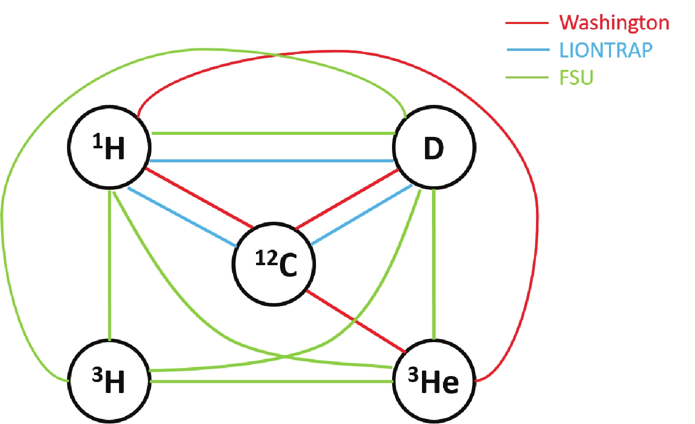
Figure 3. The connection diagram in the lightest mass region.
-
The mass of
$ ^{52} $ Co was measured firstly with the CSR-IMS in Lanzhou [2016Xu10], and the value was adopted in AME2016 as the only available experimental result. After the publication of AME2016, the JYFLTRAP group published their result for$ ^{52} $ Co [2017Ne05]. The two results deviate with each other by 2.8$ \sigma $ . In both measurements, an isomeric state of$ ^{52} $ Co was observed and can be separated fairly well from the ground state. The resolving powers of these two measurements are comparable. From the spectra in the two papers, it is difficult to identify possible problems. We keep both results in the present evaluation and appeal for new studies to solve this issue. -
This case has been discussed in AME2012 and AME2016. The Q-value for
$ ^{99} $ Rh($ \beta^+ $ )$ ^{99} $ Ru was adjusted to be 2044(7) keV in AME2016, where the$ Q_{\beta^+} $ was mainly determined from the two$ \beta $ -decay results in Ref. [1952Sc11] and [1959To25]. A higherQ-value of 2170(30) keV was reported in the later work [1974An23], but was not used in AME due to its large uncertainty. However, it was found that the Q-value should be larger than 2059.34 keV because this state was populated in beta-decay experiments.Both
$ ^{99} $ Rh and$ ^{99} $ Ru are primary nuclides in our evaluation. The mass of$ ^{99} $ Ru is mainly determined by (n,$ \gamma $ ) reaction to$ ^{100} $ Ru, which in turn is determined from Penning trap measurement. The uncertainty of the adjusted$ ^{99} $ Rh mass is 6.7 keV. The mass of$ ^{99} $ Rh can also be determined through the$ Q_{\beta^+} $ value of$ ^{99} $ Pd, which in turn is measured with a Penning trap with an uncertainty of 5.4 keV. Consequently, even if we do not use any of the experimental results from the beta-spectrum measurements of$ ^{99} $ Rh, we can still determine the Q-value of$ ^{99} $ Rh($ \beta^+ $ )$ ^{99} $ Ru to be 2032(21) keV. If we increase the Q-value of$ ^{99} $ Rh($ \beta^+ $ )$ ^{99} $ Ru, then strong tension will be built around this region.In AME2020, we discard the result from [1952Sc11]. The unweighted average of results from [1959To25] and [1974An23] is then used in the evaluation. The adjusted value is 2041(19) keV, still marginally smaller than the required decay energy, as discussed above.
-
In the AME2012 evaluation, we found large discrepancies between data coming from combinations of the very precise (n,
$ \gamma $ ) reactions with$ \beta^{+} $ ,$ \beta^{-} $ and$ \varepsilon $ decay energies versus direct Penning-trap data [2011Go23]. We finally decided at that time to provisionally not use the new Penning trap result and called for more measurements in order to clarify this issue. In the AME2016 evaluation, we were aware of the experimental results for$ ^{102} $ Pd and$ ^{103} $ Pd from the ESR mass measurements through a private communication [2014Ya.A]. Their results support the SHIPTRAP datum, although with relatively large uncertainties. We therefore decided to discard two pieces of data:$ ^{102} $ Rh($ \beta^{-} $ )$ ^{102} $ Pd and$ ^{103} $ Pd($ \varepsilon $ )$ ^{103} $ Rh, and to use the SHIPTRAP result. The local consistency was then restored.The treatment is now further supported by the recent results from JYFLTRAP [2019Ne04]. The mass difference of
$ ^{102} $ Pd and$ ^{102} $ Ru was measured using both the Time-of-Flight and the Phase-Imaging Ion Cyclotron Resonance techniques. The obtained result is around 8 times more precise and in excellent agreement with the value obtained at SHIPTRAP, verifying the reliability of the Penning trap mass spectrometry. This issue is thus considered to be resolved. -
The full content of the present issue is accessible on-line at the AMDC website [27]. In addition to several graphs representing the mass surface, beyond the main ones given in Part II, are available on the AMDC website.
Tables of masses (Part II, Table I) and nuclear reaction and separation energies (Part II, Table III) are available in ASCII format to simplify their input to computer programs. The headers of these files give information on the formats. The first file, named mass.mas20, contains the table of masses. The next two files correspond to the table of reaction and separation energies, in two parts of 6 entries each, as in Part II, Table III: rct1.mas20 for
$ S_{2n} $ ,$ S_{2p} $ ,$ Q_{\alpha} $ ,$ Q_{2\beta} $ ,$ Q_{\varepsilon p} $ and$ Q_{\beta n} $ (odd pages in this issue); and rct2.mas20 for$ S_{n} $ ,$ S_{p} $ ,$ Q_{4\beta} $ ,$ Q_{d,\alpha} $ ,$ Q_{p,\alpha} $ and$ Q_{n,\alpha} $ (facing even pages). -
This work is supported in part by the National Key Research and Development Program of China (Grant No. 2016YFA0400504), the Strategic Priority Research Program of Chinese Academy of Sciences (CAS, Grant No. XDB34000000), the U.S. Department of Energy, Office of Science, Office of Nuclear Physics, under Contract No. DE-AC02-06CH11357. W.J.H. acknowledges financial support by the Max-Planck-Society. S.N. acknowledges the support of the RIKEN Pioneering Project Funding.
We wish to thank our many colleagues who provided answers to our questions regarding specific experimental data, as well as those who sent us preprints of their work prior to publication. Continuing interest, discussions, suggestions and encouragements from D. Lunney are highly appreciated.
-
Primary data from Penning-trap measurement are typically given in the form of a frequency ratio, which is converted to a linear equation of atomic masses in the AME. The code of a Fortran program for converting frequency ratios to linear equations was given in AME2016 [2]. Here we just describe the principle of this method.
In the following, quantities with the subscript
$ {r} $ describe the characteristics of the reference ion in the Penning trap. Equivalent quantities, with no subscript, describe characteristics of the ion being measured.In AME2012 [24], the frequency ratio was described as:
$ R = \frac{f_{r}}{f} = \frac{{\cal M} - m_e\; q + B}{{\cal M}_{r} - m_e\; q_{r} + B_{r}} \; \frac{q_{r}}{q} , $

(9) This function is only valid for atoms. When molecules are involved, an extra term for the molecular binding energy should be included. Therefore in AME2016 [2], the equation was rewritten as:
$ R = \frac{f_{r}}{f} = \frac{{\cal M} - D - m_e\; q + B}{{\cal M}_{r} - D_{r} - m_e\; q_{r} + B_{r}} \; \frac{q_{r}}{q} , $

(10) where q is the charged state of the given ion, D is the molecular binding energy (dissociation energy), B is the electron binding energy,
$ m_e $ is the mass of the electron and$ {\cal M} $ the total atomic mass. All masses and energies are in atomic mass units u and so, u = 1.This expression can be written in terms of the mass excess M and atomic mass number A:
$ A + M - D -m_{e}q + B = R\frac{q}{q_{r}}(A_{r} + M_{r} - D_{r} - m_{e}q_{r} + B_{r}) $

(11) or, alternatively:
$ \begin{aligned}[b] M - R\dfrac{q}{q_{r}}M_{r} = &\, m_{e}q(1 - R) + A_{r}(\frac{q}{q_{r}}R - \frac{A}{A_{r}}) \\ & + R\dfrac{q}{q_{r}}(B_{r} - D{r}) - (B - D) . \end{aligned} $

The general aim is to establish some quantity y and its associated precision
$ dy $ . We define C to be a truncated, three-digit decimal approximation of the ratio A to$ A_{r} $ , and then we can write:$ y\; \; = \; \; M - C\; M_{r} $

(12) and so
$ y\; \; = \; \; y_1 + y_2 + y_3 + y_4 , $

(13) where
$ y_1\; \; = \; \; M_{r}\left (R\; \frac{q}{q_{r}} - C \right) , $

(14) $ y_2\; \; = \; \; m_e\; q(1 - R) , $

(15) $ y_3\; \; = \; \; A_{r} \left(\frac{q}{q_{r}}\; R - \frac{A}{A_{r}}\right) , $

(16) and
$ y_4\; \; = \; \; R\frac{q}{q_{r}}(B_{r} - D_{r}) - (B - D) . $

(17) To fix relative orders of magnitude,
$ M_r $ is generally smaller than 0.1 u,$ R - C $ is a few 10$ ^{-4} $ ,$ (1 - R) $ is usually smaller than unity (and typically 0.2 for a 20% mass change),$ R - \frac{A}{A_r} $ varies from 1 to 100$ \times 10^{-6} $ ,$ (B_{r} - D_{r}) $ is generally smaller than 0.1$ \mu $ u, and$ A_r $ is typically 100 u for atomic mass$ A = 100 $ . The four terms$ y_1 $ ,$ y_2 $ ,$ y_3 $ , and$ y_4 $ take values of the order of 10$ \mu $ u, 100$ \mu $ u, 10 to 10000$ \mu $ u, and 0.1$ \mu $ u, respectively.The associated precision
$ dy $ is written:$ dy\; \; = \; \; dy_1 + dy_2 +dy_3 + dy_4 , $

(18) where
$ dy_1\; \; = \; \; \frac{q}{q_{r}}\; M_{r}\; dR + \left (R\; \frac{q}{q_{r}} - C \right ) \; dM_r \simeq dR \times 10^5\; \mu {\rm u} , $

(19) $ dy_2\; \; = \; \; m_e\; q\; dR \simeq dR \times 10^3\; \mu {\rm u} , $

(20) $ dy_3\; \; = \; \; \frac{q}{q_{r}}\; A_{r}\; dR \simeq dR \times 10^8\; \mu {\rm u} , $

(21) and
$ \begin{aligned}[b] dy_4 = & \dfrac{q}{q_{r}}\; (B_r - D_{r})\; dR + R\; \dfrac{q}{q_{r}}(dB_r - dD_{r}) \\ & - (dB - dD) \simeq dR \times 10^{-1}\; \mu {\rm u} . \end{aligned} $

(22) Consequently, only the 3rd term contributes significantly to the precision of the measurement, and so we write:
$ dy\; \; = \; \; dy_3 $ .If the two frequencies are measured with a typical precision of
$ 10^{-7} $ for ions at$ A = 100 $ , then the precision on the frequency ratio R is$ 1.4\times 10^{-7} $ and the precision on the mass is approximatively$ 14\; \mu $ u.Next we will illustrate how to calculate the molecular binding energy for the most precise Penning trap experiment.
-
The bond dissociation energy D is a quantity which signifies the strength of a chemical bond. The bond dissociation energy for a bond A—B, which is broken through reaction:
$ \text{AB} \rightarrow \text{A + B} $

is defined as the standard enthalpy change at a specified temperature[35]:
$ D^{o}( \text{AB}) = \Delta Hf^{o}_{0}( \text{A}) + \Delta Hf^{o}_{0}({\rm B}) - \Delta Hf^{o}_{0}({\rm AB}) , $

(23) where
$ \Delta Hf^{o}_{0} $ is the standard heat of formation and its value is available for a large number of atoms and compounds on NIST Chemistry Webbook [36]. All$ D^{o} $ values refer to the gaseous state at temperature either 0 K or 298 K. When data on the standard heat of formation is absent at 0 K,$ D^{o}({\rm AB}) $ will be converted to$ D^{o}_{298}({\rm AB}) $ by the approximation:$ D^{o}_{298}({\rm AB})\approx D^{o}({\rm AB}) + 3.72 \; \rm kJ/mol . $

(24) Unlike diatomic molecules which involve only one bond, polyatomic molecules have several bonds and their D's are the sum of all the single bonds. For example, if one wants to know the dissociation energy of CH
$ _{4} $ , one needs to calculate the dissociation energy of the four bonds CH$ _{3} $ —H, CH$ _{2} $ —H, CH—H, and C—H, respectively:$ \begin{array}{l} D^{o}({\rm CH_{3}-H}) = \Delta Hf^{o}_{0}({\rm CH_{3}}) + \Delta Hf^{o}_{0}({\rm H}) - \Delta Hf^{o}_{0}({\rm CH_{4}}) ,\\ D^{o}({\rm CH_{2}-H}) = \Delta Hf^{o}_{0}({\rm CH_{2}}) + \Delta Hf^{o}_{0}({\rm H}) - \Delta Hf^{o}_{0}({\rm CH_{3}}) ,\\ D^{o}({\rm CH-H}) = \Delta Hf^{o}_{0}({\rm CH}) + \Delta Hf^{o}_{0}({\rm H}) - \Delta Hf^{o}_{0}({\rm CH_{2}}) ,\\ D^{o}({\rm C-H}) = \Delta Hf^{o}_{0}({\rm C}) + \Delta Hf^{o}_{0}({\rm H}) - \Delta Hf^{o}_{0}({\rm CH}) .\\ \end{array} $

(25) Summing over all four bonds above, we can obtain:
$ \begin{aligned}[b] D^{o}({\rm CH_{4}}) = & D({\rm CH_{3}-H}) + D({\rm CH_{2}-H}) \\ & +D({\rm CH-H}) + D({\rm C-H}) \\ = & \Delta Hf^{o}_{0}({\rm C}) + 4\times\Delta Hf^{o}_{0}({\rm H}) - \Delta Hf^{o}_{0}({\rm CH_{4}}) . \end{aligned} $

The dissociation energy can be generalized for a polyatomic molecule which has the form
$ {\rm A_{n}B_{k}C_{i}} $ :$ \begin{aligned}[b] D^{o}({\rm A_{n}B_{k}C_{i}}) = & n\Delta Hf^{o}_{0}({\rm A}) + k\Delta Hf^{o}_{0}({\rm B}) + i\Delta Hf^{o}_{0}({\rm C}) \\ & - \Delta Hf^{o}_{0}({\rm A_{n}B_{k}C_{i}}) . \end{aligned} $

(26) The ionization energies for molecules are available on NIST Atomic Spectra Database [37]. We now illustrate this treatment with one example.
-
In the work of [2004Ra33], a cyclotron frequency ratio R = 0.999421460888(7) of relative precision
$ 7 \times 10^{-12} $ has been obtained for ions$ ^{13} $ C$ _{2} $ H$ ^{+}_{2} $ and$ ^{14} $ N$ ^{+}_{2} $ . We first calculate$ D^{o}({\rm C_{2}H_{2}} $ ) by applying Eq. 26:$ \begin{aligned}[b] D^{o}({\rm C_{2}H_{2}}) = & 2 \times \Delta Hf^{o}_{0}({\rm C}) + 2 \times \Delta Hf^{o}_{0}({\rm H}) - \Delta Hf^{o}_{0}({\rm C_{2}H_{2}}) \\ = & 2 \times 716.68 + 2 \times 218.998 - 227.40 \\ =& 1641.956\; {\rm kJ/mol} \\ =& 17.018\; \rm eV . \end{aligned} $

$ D^{o}({\rm N_{2}}) = 944.9 $ kJ/mol$ = 9.793 $ eV is obtained from Ref. [38], since$ \Delta Hf^{o}_{0}({\rm N_{2}} $ ) is not on the list of [36]. Combining the ionization energy$ B({\rm C_{2}H_{2}}) = 11.400 $ eV and$ B({\rm N_{2}}) = 15.581 $ eV, we obtain the mass difference:$ \rm ^{13}C + H - ^{14}N = 8105.862995(98)\; \rm \mu {\rm u} . $

In the original paper [2004Ra33], this equation is given as:
$ \rm ^{13}C + H - ^{14}N = 8105.86288(10)\; \mu u , $

which differs by 12(10) nu from our calculation. The difference is because we used the updated molecular binding energy from Ref. [36,38]. In this case, the molecular binding energy is 170 times larger than the uncertainty, and even the updates of the molecular energies have significant impact on the deduced values.
-
In cases where two or more unresolved lines may combine into a single one in an observed spectrum, while one cannot decide which ones are present and in which proportion, a special procedure has to be used.
The first goal is to determine what is the most probable value
$ M_{exp} $ that will be observed in the measurement, and what is the uncertainty$ \sigma $ of this prediction. We assume that all the lines may contribute and that all contributions have equal probabilities. The measured mass reflects the mixing. We call$ M_0 $ the mass of the lowest line, and$ M_1, M_2, M_3, \ldots$ the masses of the other lines. For a given composition of the mixture, the resulting mass m is given by$ m = (1 - \sum\limits_{i = 1}^n {x_i}) M_0 + \sum_{i = 1}^n {x_i M_i} , \quad \rm{with} \begin{cases} 0\leq x_i\leq 1 \\\sum_{i = 1}^n{x_i}\leq 1 \end{cases} $

(27) in which the relative unknown contributions
$ x_1, x_2, x_3, \ldots$ have each a uniform distribution of probability within the allowed range.If
$ P(m) $ is the normalized probability of measuring the value m, then :$ \overline{M} = \int{P(m) m dm} $

(28) $ {\rm{and}} \ \ \ \ \sigma^2 = \int {P(m) (m-\overline{M})^2 dm} . $

(29) It is thus assumed that the experimentally measured mass will be
$ M_{exp} = \overline{M} $ , and that$ \sigma $ , which reflects the uncertainty on the composition of the mixture, will have to be quadratically added to the experimental uncertainties. -
In the case of two lines, one simply gets
$ m = (1-x_1)M_0 + x_1 M_1 \ \ \rm{with} \ \ \ 0\leq x_1 \leq 1 . $

(30) The relation between m and
$ x_1 $ is biunivocal so that$ P(m) = \begin{cases} 1/(M_1-M_0) &\rm{if} \ M_0\leq m \leq M_1, \\0 & {\rm{elsewhere}} \end{cases} $

(31) i.e. a rectangular distribution, and one obtains:
$ \begin{aligned}[b] M_{exp} = & \frac{1}{2}(M_0 + M_1) , \\ \sigma = & \frac{\sqrt{3}}{6}(M_1-M_0) = 0.290\ (M_1-M_0) . \end{aligned} $

(32) Therefore, the ground state mass
$ M_0 \pm \sigma_0 $ can be determined from the measured mass$ M_{exp} \pm \sigma_{exp} $ and the knowledge of the excitation energies$ E_1 \pm \sigma_1 $ with following equations:$ \begin{array}{l} M_0 = M_{exp} - \dfrac{1}{2}E_1 , \end{array} $

$ \begin{array}{l} \sigma^2 = \dfrac{1}{12}E_1^2 \quad {\rm{or}} \quad \sigma = 0.29 E_1 , \end{array} $

$ \begin{array}{l} \sigma_0^2 = \sigma_{exp}^2 + (\frac{1}{2}\sigma_1)^2 + \sigma^2 . \end{array} $

-
In the case of three spectral lines, we derive from Eq. 27:
$ m = (1-x_1 - x_2) M_0 + x_1 M_1 + x_2 M_2 , $

(33) $\begin{array}{l} \rm{with} \begin{cases} 0\leq x_1 \leq 1 \\ 0\leq x_2 \leq 1 \\ 0\leq x_1 + x_2 \leq 1 . \end{cases} \end{array}$

(34) After normalization, one gets:
$ P(m) = \frac{2k}{M_2-M_0} , $

(35) $ \rm{with} \; \begin{cases} k = (m-M_0)/(M_1-M_0)\ \ \rm{if} \ \ M_0\leq m\leq M_1 \\ k = (M_2-m)/(M_2-M_1)\ \ \rm{if} \ \ M_1\leq m\leq M_2 \end{cases} $

(36) and finally:
$ M_{exp} = \frac{1}{3}(M_0 + M_1 + M_2) $

(37) $ \sigma = \frac{\sqrt{2}}{6}\sqrt{M_0^2 + M_1^2 + M_2^2 - M_0 M_1 - M_1 M_2 - M_2 M_0} . \nonumber $

The ground state mass
$ M_0 \pm \sigma_0 $ can be determined from the measured mass$ M_{exp} \pm \sigma_{exp} $ and the knowledge of the excitation energies$ E_1 \pm \sigma_1 $ and$ E_2 \pm \sigma_2 $ :$ \begin{aligned}[b] M_0 = & M_{exp} - \frac{1}{3}(E_1 + E_2) , \\\sigma^2 =& \frac{1}{18}(E_1^2 + E_2^2 - E_1E_2) \\ \rm{or} \sigma =& 0.236 \sqrt{E_1^2 + E_2^2 - E_1E_2} , \\ \sigma_0^2 =& \sigma_{exp}^2 + (\frac{1}{3}\sigma_1)^2 + (\frac{1}{3}\sigma_2)^2 + \sigma^2 . \end{aligned} $

If the levels are regularly spaced,
$ i.e. $ $ E_2 = 2E_1 $ ,$ \begin{array}{l} \sigma = \dfrac{\sqrt{6}}{12} E_2 = 0.204 E_2 , \end{array} $

while for a value of
$ E_1 $ very near 0 or$ E_2 $ ,$ \begin{array}{l} \sigma = \dfrac{\sqrt{2}}{6} E_2 = 0.236 E_2 . \end{array} $

-
For more than 3 lines, one may easily infer
$ M_{exp} = \sum_{i = 0}^n M_i/(n+1) $ , but the determination of$ \sigma $ requires the knowledge of$ P(m) $ . As the exact calculation of$ P(m) $ becomes rather difficult, it is more simple to do simulations.However, care must be taken that the values of the
$ x_i $ 's are explored with an exact equality of chance to occur. For each set of$ x_i $ 's, m is calculated, and the histogram$ N_j(m_j) $ of its distribution is built. Calling$ nbin $ the number of bins of the histogram, one gets :$ P(m_j) = \frac{N_j}{\sum_{j = 1}^{nbin}N_j} , $

(38) and
$ \begin{aligned}[b] M_{exp} & = \sum\limits_{j = 1}^{nbin}P(m_j)m_j , \\ \sigma^2 & = \sum\limits_{j = 1}^{nbin}P(m_j)(m_j - M_{exp})^2 . \end{aligned} $

For three excited isomers, the ground state mass
$ M_0 \pm \sigma_0 $ can be determined from the measured mass$ M_{exp} \pm \sigma_{exp} $ and the knowledge of the excitation energies$ E_1 \pm \sigma_1 $ ,$ E_2 \pm \sigma_2 $ and$ E_3 \pm \sigma_3 $ as:$ \begin{aligned}[b] M_0 = & M_{exp} - \dfrac{1}{4}(E_1 + E_2 + E_3) , \\ \sigma_0^2 = & \sigma_{exp}^2 + (\dfrac{1}{4}\sigma_1)^2 + (\dfrac{1}{4}\sigma_2)^2 + (\dfrac{1}{4}\sigma_3)^2 + \sigma^2 . \end{aligned} $

An example of a Fortran program based on the CERN library was given for the cases of two, three and four lines in AME2016 [2].
-
Conventionally, the total energy released in
$ \alpha $ decay,$ Q_{\alpha} $ , is defined as the difference between the atomic masses of the mother and daughter nuclides:$ Q_\alpha = M_{\rm mother} - M_{\rm daughter} - M_{^4\rm{He}} . $

(39) This value equals the sum of the observed energy of the
$ \alpha $ particle and that of the recoiling nuclide (with only a minor correction for the fact that the cortège of atomic electrons in the latter may be in an excited state). Unfortunately, some authors in the literature quote$ Q_\alpha $ as a value 'corrected for screening', which essentially means that they take the masses of bare nuclides for the M values in the above equation.A similar bad habit has been observed for some published proton-decay energies. We very strongly object to this custom; at the very least, the symbol Q should not be used for the difference in nuclear masses.
High precision
$ \alpha $ -decay energiesThe most precise
$ \alpha $ -decay energies are those measured absolutely using magnetic spectrographs, as summarized in Ref. [1991Ry01] and references therein. All$ \alpha $ -energy standards are determined using this method. The relation between the$ \alpha $ -particle energy$ E_{\alpha} $ and the decay energy,$ Q_{\alpha} $ is:$ Q_{\alpha} = (M-m_{\alpha}) - \sqrt{(M-m_{\alpha})^{2}-2\times M\times E_{\alpha}} + 78.6\; {\rm eV} . $

(40) where M is the mass of the parent nuclide,
$ m_{\alpha} $ is the mass of the doubly ionized$ \alpha $ particle and 78.6 eV is the binding energy of two electrons in helium. This formula had been discussed in AME1977 and has been used since then. The electron binding energy of helium has just been taken into account since AME2016.
The AME 2020 atomic mass evaluation (I). Evaluation of input data, and adjustment procedures
- Received Date: 2021-01-19
- Available Online: 2021-03-15
Abstract: This is the first of two articles (Part I and Part II) that presents the results of the new atomic mass evaluation, AME2020. It includes complete information on the experimental input data that were used to derive the tables of recommended values which are given in Part II. This article describes the evaluation philosophy and procedures that were implemented in the selection of specific nuclear reaction, decay and mass-spectrometric data which were used in a least-squares fit adjustment in order to determine the recommended mass values and their uncertainties. All input data, including both the accepted and rejected ones, are tabulated and compared with the adjusted values obtained from the least-squares fit analysis. Differences with the previous AME2016 evaluation are discussed and specific examples are presented for several nuclides that may be of interest to AME users.


 DownLoad: