


 Abstract
 HTML
HTML Reference
 Related
 PDF
PDF


-
Parton distribution functions (PDFs) and fragmentation functions (FFs) provide essential input for accurate determination of various quantities of QCD and the Standard Model [1-3] within the framework of QCD factorization [4]. While PDFs and FFs are intrinsically non-perturbative objects, their scale evolution obeys the Dokshitzer-Gribov-Lipatov-Altarelli-Parisi (DGLAP) equations [5-7]. The corresponding evolution kernels are space-like (
$ q^2 < 0 $ , Fig. 1(a)) splitting functions for PDFs and time-like ($ q'^2 > 0 $ , Fig. 1(b)) splitting functions for FFs, both of which can be calculated in QCD perturbation theory. Determining the splitting functions to higher orders is one of the most important tasks of perturbative QCD.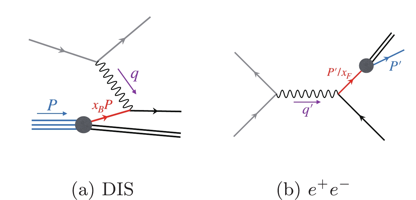
Figure 1. (color online) Typical processes used for the determination of PDFs (a) and FFs (b).
Space-like splitting functions were obtained to next-to-next-to-leading order (NNLO) some time ago [8,9], and have more recently been obtained to N3LO for non-singlet functions [10]. However, knowledge for time-like splitting functions is less precise. Direct calculation of time-like splitting functions has been done at NLO in Ref. [11]. At NNLO and beyond, results by direct calculation are not yet available (see Refs. [12-15] for recent progress). However, it has long been noted that space-like deep inelastic scattering (DIS) and
$ e^+e^- $ annihilation are kinematically related [16,17]. The easiest way to see this is from the definition of the Bjorken variable$ x_B $ in DIS and the Feynman variable$ x_F $ in$ e^+e^- $ ,$ x_B = \frac{-q^2}{2 P \cdot q} \,, \qquad x_F = \frac{2 P' \cdot q'}{q'^2} \,, $

(1) where
$ P $ is the incoming hadron momentum in DIS,$ P' $ is the detected hadron momentum in$ e^+e^- $ , and$ q $ and$ q' $ are the space-like and time-like momentum transfer, respectively. After crossing,$ P = - P' $ ,$ q = q' $ , one finds the analytic continuation relation$ x_B = 1/x_F $ . However, beyond LO, the analytic continuation relation cannot be applied directly to the splitting functions, but to the appropriate bare quantities [11,18]. Analytic continuation of exclusive amplitudes has also been understood at NLO accuracy [19]. Further subtleties arise at NNLO, where additional momentum sum rules, supersymmetry relations, and reciprocity considerations at large$ x $ [20] are needed in order to obtain NNLO non-singlet and singlet time-like splitting functions [21-23]. However, as has been explicitly pointed out in Ref. [23], the third-order corrections to off-diagonal quark-gluon splitting,$ P_{qg}^{{\rm{T}},(2)} $ , have only been determined up to an uncertainty proportional to the QCD beta function. Fixing this remaining uncertainty is not only crucial for achieving complete NNLO analysis of parton-to-hadron fragmentation, but is also important for precision jet substructure studies, see e.g. Refs. [24-31].In this Letter we study the analytic continuation of splitting functions using soft-collinear effective theory [32-35]. We point out that splitting functions, both space-like and time-like, can be extracted from bare transverse-momentum-dependent (TMD) distributions. We identify the origin of the breakdown of direct analytic continuation for splitting functions and TMD distributions, as they are computed from the squares of splitting amplitudes, and are therefore not analytic. Nevertheless, we identify certain holomorphic and anti-holomorphic contributions to TMD distributions, for which a correct rule of analytic continuation can be established. We use this to obtain time-like splitting functions at NNLO from the space-like ones. Our results are in full agreement with those obtained in Refs. [21-23], except for a minor discrepancy in
$ P_{qg}^{{\rm{T}},(2)} $ . Finally, we propose an all-order generalization of the Gribov-Lipatov reciprocity relation [36] for singlet splitting functions in QCD. Using the time-like splitting functions obtained in this work, we verify this relation to NNLO, where the discrepancy in$ P_{qg}^{{\rm{T}},(2)} $ mentioned above plays an important role. -
TMD distributions are central ingredients in the TMD factorization approach to hard scattering [37-48]. In SCET, they can be conveniently defined as matrix elements of collinear fields integrated over light-cone coordinates. Since for the purpose of analytic continuation, there is no intrinsic difference between quark and gluon TMD distributions, we shall focus on quark TMD distributions in the discussion below. The operator definition for quark TMD PDFs is given by
$\begin{aligned}[b] {\cal{B}}_{q/N}(x_B,b_\perp) =& \sum\limits\int\limits_{X_n} \int \frac{{\rm d}b^-}{2\pi} \, {\rm e}^{-{\rm i} x_B b^- P^+} \\ &\cdot \langle N(P) | \bar{\chi}_n(0,b^-,b_\perp) | X_n \rangle \frac{\not{\bar{n}}}{2} \langle X_n| \chi_n(0) | N(P) \rangle \,, \end{aligned}$

(2) where
$ N(P) $ is a hadron state with momentum$P^\mu = (\bar{n} \cdotP) n^\mu/2 = P^+ n^\mu/2$ , with$ n^\mu = (1, 0, 0, 1) $ and$\bar{n}^\mu = (1, 0, 0, -1)$ .$ \chi_n(x) = W^\dagger_n(x) \xi_n(x) $ is the gauge-invariant collinear quark field [49], and$ W^\dagger_n(x) = {\cal{P}} \exp{\left({\rm i} g_s \int_0^{\infty} {\rm d}s \, \bar{n} \cdot{{A}}_n(x + s \bar{n} ) {\rm e}^{-\varepsilon s}\right)} $

(3) is the path-ordered
$ n $ -collinear Wilson lines in the fundamental representation. Although not necessary, we have inserted a complete set of$ n $ -collinear states$ \mathbb{1} = {\sum\nolimits_{X_n}\int}\quad | X_n \rangle \langle X_n | $ into the definition of$ {\cal B}_{q/N} $ . Similarly, for an anti-quark$ \bar{q} $ fragmenting into an anti-hadron$ \overline{N} $ , the TMD FF can be written as$\begin{aligned}[b] & {\cal{F}}_{\overline N/\bar q}(x_F,b_\perp) ={\sum\limits\int\limits_{X_n}} x_F^{1-2 \epsilon} \int \frac{{\rm d}b^-}{2\pi} {\rm e}^{{\rm i} b^- P'^+ / x_F} \\& \quad \times \langle 0 | \bar \chi_{n}(0,b^-,b_\perp) | \overline N(P'),X_n \rangle \frac{\not{\bar{n}}}{2} \langle \overline N(P'),X_n | \chi_{n}(0) | 0 \rangle \,,\end{aligned} $

(4) where
$ P'^\mu = (\bar n \cdotP') n^\mu/2 = P'^+ n^\mu/2 $ is the momentum of the final-state detected hadron. At high energy and small$ |\vec{b}_\perp| $ , TMD PDFs and FFs admit light-cone operator product expansion onto collinear PDFs and FFs, with perturbative calculable Wilson coefficients, which have been calculated to NNLO [50-58], and very recently to N3LO [59,60]. The Wilson coefficients can be directly calculated by replacing the non-perturbative hadronic state$ N\,(\overline{N}) $ by the perturbative partonic state$ i\,(\bar \imath) $ , namely$ {\cal B}_{q/i} $ and$ {\cal F}_{\bar \imath/\bar q} $ . The operator definitions in Eqs. (2) and (4) make it clear that they can be computed from squared amplitudes integrated over collinear phase space [61],$ \begin{aligned}[b] {\cal B}_{q/i} =& \sum\limits_{X_n} \int{\rm d} {\rm{PS}}_{X_n} {\rm e}^{- {\rm i} K_\perp\cdot b_\perp} \delta(K^+ - (1 - x_B) P^+) \\ &\times {\bf{Sp}}_{X_n q^* \leftarrow i}^{\rm{S}} \frac{\not{\bar{n}}}{2} {\bf{Sp}}_{X_n q^* \leftarrow i}^{{\rm{S}},*} \,, \\ {\cal F}_{\bar \imath/\bar q} =& \sum\limits_{X_n} x_F^{1 - 2 {\epsilon}} \int{\rm d}{\rm{PS}}_{X_n} {\rm e}^{- {\rm i} K_\perp\cdot b_\perp} \delta\left(K^+ - \left(\frac{1}{x_F} - 1 \right) P'^+\right) \\ &\times {\bf{Sp}}_{X_n \bar \imath \leftarrow \bar q^*}^{\rm{T}} \frac{\not{\bar{n}}}{2} {\bf{Sp}}_{X_n \bar \imath \leftarrow \bar q^*}^{{\rm{T}},*} \,, \end{aligned} $

(5) where
$ K^\mu $ is the total momentum of$ |X_n \rangle $ , and$ {\rm d}{\rm{PS}}_{X_n} $ is the collinear phase space measure. We also define the (generalized) space-like and time-like splitting amplitudes [62,63],$ \begin{aligned}[b] {\bf{Sp}}_{X_n q^* \leftarrow i}^{\rm{S}} \left( k_a^+/P^+, \dots \right) =& \ \langle X_n| \chi_n(0) | V_{P_l}^i(P_r) \rangle \,, \\ {\bf{Sp}}_{X_n \bar \imath \leftarrow \bar q^*}^{\rm{T}} (k_a^+/P'^+, \dots) =& \ \langle X_n, V_{P'_l}^{\bar \imath}(P'_r) | \chi_{n}(0) | 0 \rangle \,, \end{aligned} $

(6) where
$ {\bf{Sp}}_{X_n q^* \leftarrow i}^{\rm{S}} $ denotes the amplitudes for parton$ i $ splitting into an off-shell quark$ q^* $ and$ X_n $ , and similarly for$ {\bf{Sp}}_{X_n \bar \imath \leftarrow \bar q^*}^{\rm{T}} $ .$ |V_{P_l}^i(P_r) \rangle $ denotes the partonic state$ i $ with momentum$ P $ , decomposed into label momentum and residual momentum$ P^\mu = P^\mu_l + P^\mu_r $ , and similarly for$ V_{P'_l}^{\bar \imath}(P'_r) $ . Label momentum in SCET is Euclidean-like and does not require causal prescription, while residual momentum does and will be discussed in the next section. When$ X_n $ consists of a single parton, Eq. (6) reduces to the usual$ 1{\rightarrow} 2 $ splitting amplitudes, which are known to two-loop accuracy [64-66]. Results are also available for$ 1{\rightarrow} 3 $ and$ 1{\rightarrow} 4 $ splitting [67-70]. In Eq. (6) we have made explicit the possible functional dependence on$ P^+ $ and$ P'^+ $ , where$ k_a $ is any combination of momenta in$ |X_n\rangle $ . This is due to reparameterization III invariance in SCET [71], namely the SCET matrix element should be invariant under$ n^\mu {\rightarrow} e^{\lambda} n^\mu $ and$ \bar{n}^\mu {\rightarrow} e^{-\lambda} \bar{n}^\mu $ . We have also made implicit in Eq. (5) the averaging over initial-state spin and color, as well as the sum over final-state spin and color.After proper renormalization and zero-bin subtraction [72], the TMD PDFs and FFs still contain collinear divergence due to the tagged hadron in the initial state or final state. Schematically, at
$ n $ -th order in perturbation theory, the single pole of the remaining collinear divergences has the following convolution form:$ {\cal B}_{q/i}^{(n)} \sim \sum\limits_j \frac{P_{qj}^{{\rm{S}}, (n)}}{n {\epsilon}} \otimes \phi_{ji}^{\rm{bare}} \,, \quad {\cal F}_{\bar \imath /\bar q}^{(n)} \sim \sum\limits_j d_{\bar \imath j}^{\rm{bare}} \otimes \frac{P_{j \bar q}^{{\rm{T}},(n)}}{n {\epsilon}} \,, $

where
$ \phi_{ij}^{\rm{bare}} = d_{ij}^{\rm{bare}} = \delta_{ij} $ are the bare partonic PDFs and FFs. Therefore, one can extract the space-like and time-like splitting functions directly from the partonic TMD PDFs and FFs. -
In order to understand the analytic continuation for TMD PDFs and FFs, we start with LSZ reduction on the space-like splitting amplitudes:
$ {\bf{Sp}}_{X_n q^* \leftarrow i}^{\rm{S}}= \int{\rm d}^dx \, {\rm e}^{-{\rm i} P_r \cdot x} \langle X_n |{\rm{T}} \{ \chi_n (0) J_{P_l}^i(x) \} | 0 \rangle \,, $

(7) where the current
$ J^{i}_{P_l}(x)=i(i{\cal{P}}_l+\partial_x)^2 V_{P_l}(x) $ creates a parton state$ i $ from vacuum. Using the fact that the SCET operator$ \chi_n(x) $ is local in residual space, the time-ordering product can be replaced by a (anti-)commutator if$ i $ is a boson (fermion),$ {\rm{T}}\{\chi_n(0)J^{i}_{P_l}(x)\} = \theta(-x^0)\left[\chi_n(0),J^{i}_{P_l}(x)\right]_{\mp} \pm J^{i}_{P_l}(x)\chi_n(0) \,. $

(8) The second term in Eq. (8) does not contribute to the correlator since
$ \chi_n(0) $ effectively carries negative energy in the physical process and thus annihilates vacuum$ | 0 \rangle $ . Note that since$ \chi_n $ is local, the (anti-)commutator in Eq. (8) vanishes in the space-like region$ \Omega_0 $ of Fig. 2. Thus, we can rewrite the space-like splitting amplitudes as: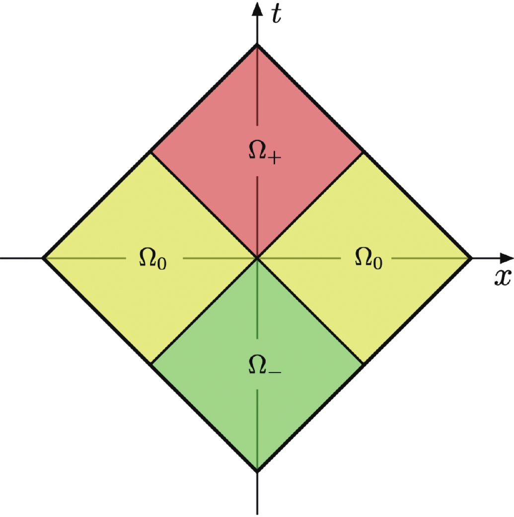
Figure 2. (color online) Penrose diagram of Minkowski space.
$ {\bf{Sp}}_{X_n q \leftarrow i}^{\rm{S}}=\int\limits_{x \in \Omega_-}{\rm d}^dx \, {\rm e}^{-{\rm i} P_r \cdot x} \langle X_n | [ \chi(0), J_{P_l}^i(x) ]_{\mp} | 0 \rangle \,, $

(9) where the
$ x $ integral is now restricted to inside the past light-cone,$ \Omega_- $ . Demanding analyticity for the splitting amplitudes imposes a unique causal prescription for residual momenta,$ P_r{\rightarrow} P_r+i q_I $ where$ q_I $ is any positive-energy time-like vector.Similarly, we can write the time-like splitting amplitudes as
$ {\bf{Sp}}_{X_n \bar \imath \leftarrow \bar q}^{\rm{T}} = \int\limits_{x \in \Omega_+}{\rm d}^d x \, {\rm e}^{{\rm i} P'_r \cdot x} \langle X_n | [ J_{P'_l}^{\bar \imath}(x) , \chi(0) ]_{\mp} | 0 \rangle \,, $

(10) and again the causal prescription must be
$ P^\prime_r {\rightarrow} P^\prime_r + i q_I $ . With the causal prescription properly defined, we can now discuss the analytic continuation between space-like and time-like splitting amplitudes.Since splitting amplitudes are analytic functions of external momentum, we can continue
$ P $ and$ P' $ to a common space-like infinity region, where space-like and time-like splitting amplitudes can be shown to equal. Therefore, by the edge-of-the-wedge theorem [73], space-like and time-like splitting amplitudes are actually analytic continuations of each other, although the causal prescription described above tells us their analytic regions are disjoint.For concreteness and later convenience, we choose a particular path displayed in Fig. 3 as the blue lines (solid and dashed), where we analytically continue the momentum of a time-like splitting amplitude from
$ P' $ (red) to$ -P' $ (green). The orange segment of the path, sitting at space-like infinity relative to$ O $ , lies inside the region where$ {\bf{Sp}}^{\rm{S}}(-P^\prime)={\bf{Sp}}^{\rm{T}}(P^\prime) $ and does not require a causal prescription. Along the red segment,$ P^\prime $ in$ {\bf{Sp}}^{\rm{T}}(P^\prime) $ should have positive imaginary part$ {\rm{Im}} P^\prime\in \Omega_{+}^{p} $ , while along the green segment,$ P^\prime $ in$ {\bf{Sp}}^{\rm{S}}(-P^\prime) $ should have a negative imaginary part$ {\rm{Im}}P^\prime\in\Omega_{-}^{p} $ . In principle, every path allowed by analytic continuation should serve the same purpose.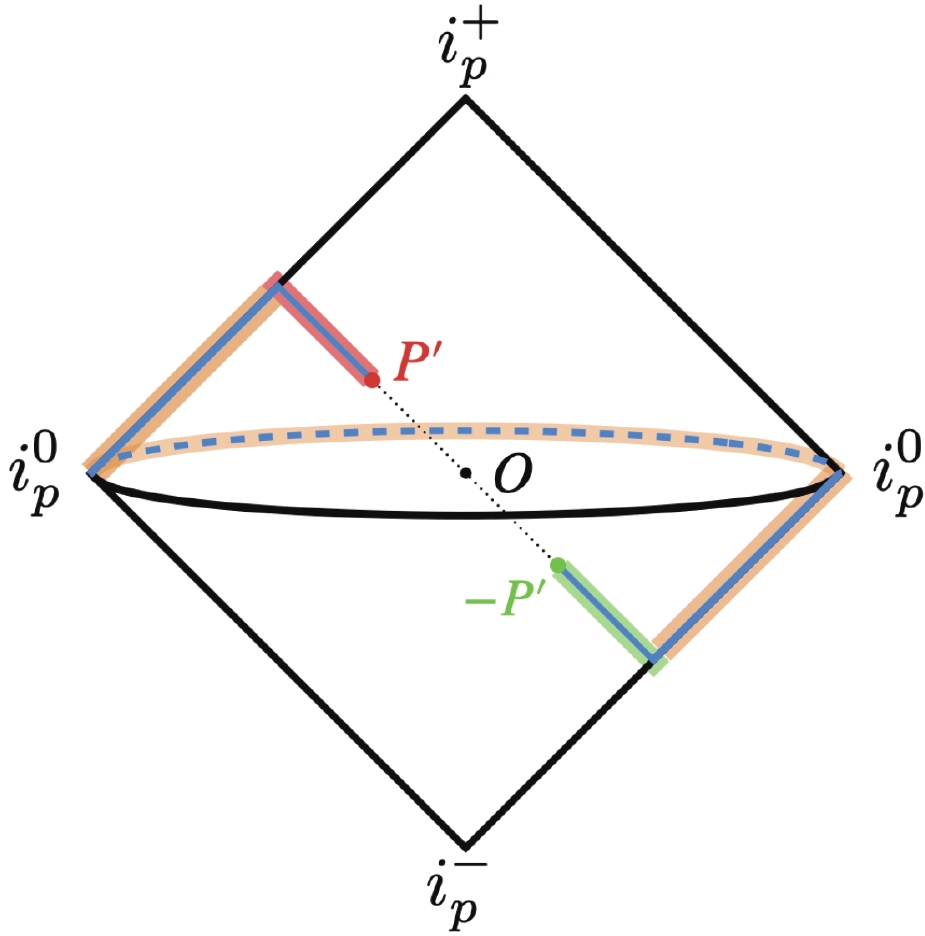
Figure 3. (color online) Penrose diagram of real momentum space. We have shown an extra spatial momentum dimension to visualize the path of analytic continuation, the blue lines.
The corresponding contour in the complex
$ 1/{P^\prime}^{+} $ plane is depicted schematically in Fig. 4. Note that the orange segment in Fig. 3 cannot be simply shown in this plane of a single variable, so we abstractly use an orange dot at the origin to represent it, which allows us to cross the real line analytically. The physical region of the time-like process sits just below the positive real line with an infinitesimal imaginary part, while the physical region of the space-like process is just above the negative real line. As illustrated in Fig. 4, the correct path connects${\rm e}^{-{\rm i}0_+}/{P^\prime}^{+}$ and${\rm e}^{-{\rm i}\pi-{\rm i}0_+}/{{P^\prime}^+}$ for positive$ {P^\prime}^+ $ .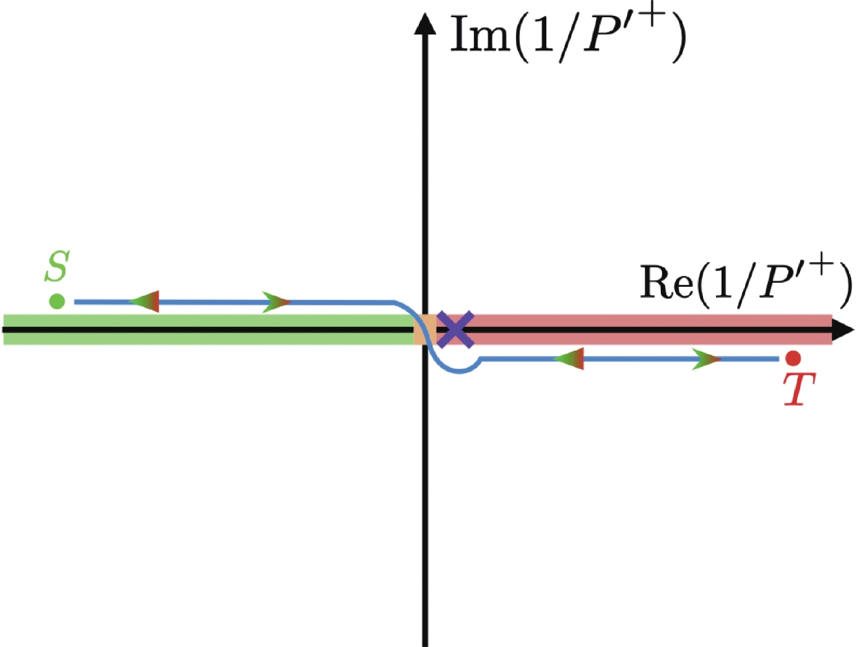
Figure 4. (color online) Path of analytic continuation from a time-like point T to a space-like point S or vice versa in the
$ 1/{P^\prime}^{+} $ plane.The discussion above determines a unique prescription for the analytic continuation of splitting amplitudes. We define an operator
$ \underset{{\rm{T}} {\rightarrow} {\rm{S}}}{\cal{AC}} $ which continues a time-like splitting amplitude from its physical region to a space-like splitting amplitude as$ \begin{aligned}[b] \underset{{\rm{T}} {\rightarrow} {\rm{S}}}{\cal{AC}} \circ {\bf{Sp}}_{X_n \bar \imath \leftarrow \bar q}^{\rm{T}} \left(\frac{k_a^+}{P'^+ {\rm e}^{{\rm i}0_+}}, \cdots \right) \equiv & {\bf{Sp}}_{X_n \bar \imath \leftarrow \bar q}^{\rm{T}} \left(\frac{k_a^+}{P'^+ {\rm e}^{{\rm i} (\pi +0_+)}}, \cdots \right) \\ =& {\bf{Sp}}_{X_n q \leftarrow i}^{\rm{S}} \left(\frac{k_a^+}{P^+ {\rm e}^{{\rm i}0_+}}, \cdots\right) \,. \end{aligned} $

(11) Similarly for a space-like to time-like continuation,
$ \begin{aligned}[b] \underset{{\rm{S}} {\rightarrow} {\rm{T}}} {\cal{AC}} \circ {\bf{Sp}}_{X_n q \leftarrow i}^{\rm{S}} \left(\frac{k_a^+}{P^+ {\rm e}^{{\rm i}0_+}}, \cdots \right) \equiv & {\bf{Sp}}_{X_n q \leftarrow i}^{\rm{S}} \left( \frac{k_a^+}{P^+ {\rm e}^{-{\rm i} \pi+i0_+}}, \cdots\right) \\ =& {\bf{Sp}}_{X_n \bar \imath \leftarrow \bar q}^{\rm{T}} \left(\frac{k_a^+}{P'^+ {\rm e}^{{\rm i}0_+}}, \cdots \right) \,. \end{aligned} $

(12) One can also define an analytic continuation operator for complex conjugate amplitudes,
$ \overline{\underset{{\rm{T}} {\rightarrow} {\rm{S}}}{\cal{AC}}} $ , which amounts to first performing analytic continuation to amplitudes, and then taking complex conjugates. For a tree-level amplitude,$ \underset{{\rm{T}} {\rightarrow} {\rm{S}}}{\cal{AC}} $ and$ \overline{\underset{{\rm{T}} {\rightarrow} {\rm{S}}}{\cal{AC}}} $ become identical. -
Since TMD distributions are obtained from squared amplitudes, analyticity in external momentum is lost. However, for a subset of contributions to TMD distributions at each perturbative order, it is possible to restore analyticity. We define the holomorphic part of TMD PDFs (the anti-holomorphic part is simply the conjugate of the holomorphic part) as:
$ \begin{aligned}[b] {\cal B}_{q/i}^{h} =& \int{\rm d} {\rm{PS}}_{X_n} {\rm e}^{-{\rm i} K_\perp\cdot b_\perp} \delta(K^+ - (1 - x_B) P^+) \\ &\times {\rm e}^{- \frac{b_0 \tau}{2} |K^-|} \, {\bf{Sp}}_{X_n q^* \leftarrow i}^{\rm{S}} \left(k_a^+/P^+, \dots \right) \frac{\not{\bar n}}{2} {\bf{Sp}}_{X_n q^* \leftarrow i}^{{\rm{S}}, (0), *} \,, \end{aligned} $

(13) where
$ {\bf{Sp}}^{{\rm{S}}, (0) ,*} $ is the complex conjugate of the tree-level splitting amplitude. We have also inserted a rapidity regulator into the definition of the TMD PDFs, which we choose to be an exponential regulator${\rm e}^{- b_0 \tau |K^-|/2}$ [55,74]. The advantage of this regulator is that all the end-point$ \delta(1-x) $ terms are absorbed into the soft function [75,76], which can be shown to be the same for Drell-Yan, DIS, or$ e^+e^- $ processes [75,77,78]. We emphasize that the results for splitting functions are independent of rapidity regularization. In the following, we shall restrict our discussion to$ 0<x<1 $ , and show that$ {\cal B}_{q/i}^h $ can be analytically continued to$ {\cal F}_{\bar \imath/\bar{q}}^h $ , and vice versa.We introduce a dimensionless light-cone momentum fraction
$ y_a = k_a^+/((1-x_B)P^+) $ . For$ X_n $ consisting of$ m $ massless partons, the holomorphic part is$ {\cal B}_{q/i}^{h,m}(x_B, |P^+|, b_\perp) = \int \prod\limits_{a = 1}^m \frac{{\rm d}^{d-2} \vec{k}_{a,\perp}}{2 (2 \pi)^3} \frac{{\rm d}y_a}{y_a} {\rm e}^{-{\rm i} K_\perp\cdot b_\perp - \frac{b_0\tau}{2} |K^-|} \frac{\delta\left(\displaystyle\sum\nolimits_{l = 1}^m y_l - 1\right) }{|1-x_B| |P^+| } {\bf{Sp}}_{X_n q^* \leftarrow i}^{\rm{S}} \left(\frac{y_a(1-x_B)}{{\rm e}^{{\rm i}0+}}, \dots \right) \frac{\not{\bar n}}{2} {\bf{Sp}}_{X_n q^* \leftarrow i}^{({\rm{S}}, (0) ,*} \,, $

(14) where in terms of dimensionless light-cone momentum fraction
$ |K^-| = |\sum\nolimits_b \vec{k}_{b,\perp}^2 y_b^{-1}|/(|1-x_B| |P^+|) $ . The additional$ |P^+| $ dependence in the argument of$ {\cal B} $ results from rapidity regularization. The analytic continuation reads$ \underset{{\rm{S}} {\rightarrow} {\rm{T}}}{\cal{AC}} \circ {\cal B}_{q/i}^{h,m} = \ \int \prod\limits_{a = 1}^m \frac{{\rm d}^{d-2} \vec{k}_{a,\perp}}{2 (2 \pi)^3} \frac{{\rm d}y_a}{y_a} {\rm e}^{-{\rm i} K_\perp\cdot b_\perp - \frac{b_0 \tau}{2} |K^-| } \frac{\delta\left(\displaystyle\sum\nolimits_{l = 1}^m y_l - 1\right) }{|1-x_B| |P^+| } {\bf{Sp}}_{X_n q^* \leftarrow i}^{\rm{S}} \left(\frac{y_a(1-x_B)}{{\rm e}^{{\rm i}(\pi+0_+)}}, \dots \right) \frac{\not{\bar n}}{2} {\bf{Sp}}_{X_n q^* \leftarrow i}^{{\rm{S}}, (0), *} $

(15) $ \quad\quad\quad\quad = \ \int \prod\limits_{a = 1}^m \frac{{\rm d}^{d-2} \vec{k}_{a,\perp}}{2 (2 \pi)^3} \frac{{\rm d}y_a}{y_a} {\rm e}^{-{\rm i} K_\perp\cdot b_\perp - \frac{b_0 \tau}{2} |K^-| } \frac{\delta\left(\displaystyle\sum\nolimits_{l = 1}^m y_l - 1\right) }{|1-x_B| |P^+| } {\bf{Sp}}_{X_n \bar \imath \leftarrow \bar{q}^*}^{\rm{T}} \left(\frac{y_a(1-x_B) }{{\rm e}^{{\rm i}0_+}}, \dots \right) \frac{\not{\bar n}}{2} {\bf{Sp}}_{X_n \bar \imath \leftarrow \bar{q}^*}^{{\rm{T}}, (0), *} \,. $

(16) Note that the analytic continuation operator only acts on the all-order splitting amplitude, as well as the conjugate of the tree-level splitting amplitude. We can also write down the holomorphic part of the TMD FFs,
$ {\cal F}_{\bar \imath/\bar{q}}^{h,m}(x_F, |P'^+|,b_\perp) = \ x_F^{1-2 {\epsilon}} \int \prod\limits_{a = 1}^m \frac{{\rm d}^{d-2} \vec{k}_{a,\perp}}{2 (2 \pi)^3} \frac{{\rm d}y'_a}{y'_a} {\rm e}^{-{\rm i} K_\perp\cdot b_\perp - \frac{b_0 \tau}{2} |K^-|} \frac{\delta\left(\displaystyle\sum\nolimits_{l = 1}^m y'_l - 1\right) }{|1/x_F - 1| |P'^+| } {\bf{Sp}}_{X_n \bar \imath \leftarrow \bar{q}^*}^{\rm{T}} \left(\frac{y'_a\left(\dfrac{1}{x_F}-1\right)}{{\rm e}^{{\rm i}0+}}, \dots \right) \frac{\not{\bar n}}{2} {\bf{Sp}}_{X_n \bar \imath \leftarrow \bar{q}^*}^{{\rm{T}}, (0), *} \,, $

(17) where the lightcone momentum fraction is
$ y'_a = k_a^+/ ((1/x_F - 1)P'^+) $ ,$ |K^-| = |\sum\nolimits_b \vec{k}_{b,\perp}^2 y_b'^{-1}|/(|1/x_F-1| |P'^+| ) $

and we identify the path for analytic continuation
$ (1 - x_B) {\rightarrow} \left( \frac{1}{x_F} - 1\right) {\rm e}^{{\rm i} \pi} \,. $

(18) The analytic continuation between
$ {\cal B}^h $ and$ {\cal F}^h $ then reads$ {\cal F}_{\bar \imath/\bar{q}}^{h,m}(x_F, |P'^+|, b_\perp) = (-1)^{i_F} x_F^{1-2 {\epsilon}} {\cal B}_{q/i}^{h,m} \left( - \frac{{\rm e}^{{\rm i}\pi}}{x_F}, |P'^+|, b_\perp \right) \,, $

(19) where
$ i_F = 1 $ if$ i $ is a fermion, and 0 if a boson. The minus sign is due to crossing a fermion from initial state to final state. Similarly for gluon TMD distributions, the analytic continuation reads$ {\cal F}_{\bar \imath/g}^{h,m}(x_F, |P'^+|, b_\perp) = \ (-1)^{ 1 + i_F} x_F^{1-2 {\epsilon}} \\ \ \cdot {\cal B}_{g/i}^{h,m} \left( - \frac{{\rm e}^{{\rm i}\pi}}{x_F}, |P'^+|, b_\perp \right) \,, $

(20) where the additional minus sign originates from the operator definition, and we have suppressed the irrelevant Lorentz indices. We stress that the analytic continuation is for bare quantities before PDF or FF renormalization.
We can now apply the analytic continuation rules in Eqs. (19) and (20) to the TMD PDFs. At NLO and NNLO, there are only holomorphic and anti-holomorphic contributions. Therefore the analytic continuation rules determine the TMD FFs completely. At N3LO, the partonic contributions can be decomposed into triple real (RRR), double-real virtual (VRR), double-virtual real (VVR), and virtual-squared real (VV*R) components, as depicted in Fig. 5. The first three contributions are either holomorphic or anti-holomorphic. But the last contribution, VV*R, mixes holomorphic and anti-holomorphic terms, and therefore cannot be determined from analytic continuation. Since this is a relatively simple contribution, we can calculate it directly using the defining equation in Eq. (5). In this way we obtain the bare TMD FFs at N3LO. The results for N3LO TMD FFs will be presented elsewhere. Here we focus on splitting functions. From the single-pole terms of the bare TMD FFs we extract all the time-like splitting functions through NNLO. Comparing the results with those in the literature, we find full agreement except for the non-diagonal quark-gluon splitting. The discrepancy between our results and those presented in Ref. [23] can be written as
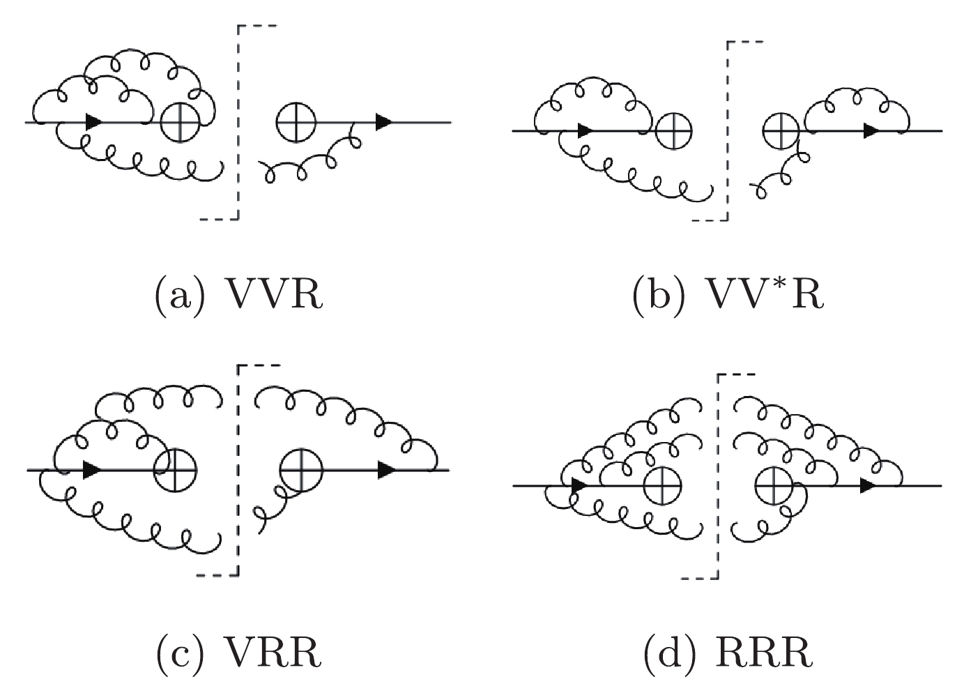
Figure 5. Contributions from different partonic channels to TMD PDFs at N3LO.
$ \begin{aligned}[b] \Delta P_{qg}^{{\rm{T}},(2)}(x) =&P_{qg}^{{\rm{T}},(2)}\Big|_{\rm{this \;work}} - P_{qg}^{{\rm{T}},(2)}\Big|_{[23]} \\=& \frac{\pi^2}{3} (C_F - C_A) \beta_0 \left[ -4 + 8 x + x^2\right. \\&\left.+ 6 (1 - 2 x + 2 x^2) \ln x \right] \,, \end{aligned} $

(21) where
$ P_{qg}^{{\rm{T}},(2)} $ is the coefficient of$ \alpha_s^3/(4 \pi)^3 $ in the off-diagonal singlet splitting matrix, and$ \beta_0 = 11 C_A/3 - 2 n_f/3 $ is the one-loop QCD beta function. In Mellin moment space the discrepancy reads$ \begin{aligned}[b]& - \int_0^1 {\rm d}x\, x^{N-1} \Delta P_{qg}^{{\rm{T}},(2)} (x) = (C_A - C_F) \beta_0 \frac{\pi^2}{3} \left( \frac{12}{(N+1)^2} \right. \\ &\left. \quad - \frac{6}{N^2} - \frac{12}{(N+2)^2} - \frac{4}{N} + \frac{8}{N+1} + \frac{1}{N+2} \right) . \end{aligned} $

(22) Note that the discrepancy vanishes for
$ N = 2 $ , as it is completely fixed by the momentum sum rule [22]. In the Appendix we point out potential sources of the discrepancy. For the convenience of the reader we provide the full time-like splitting functions through NNLO as an ancillary file along with the arXiv submission. -
With the full space-like and time-like splitting functions, it is interesting to explore yet another relation between them, the so-called reciprocity relation. Reciprocity for tree-level splitting functions was first proposed by Gribov and Lipatov [36], and says that
$ P_{ab}^{{\rm{S}},(0)}(x) = P_{ab}^{{\rm{T}},(0)}(x) $ . While the Gribov-Lipatov reciprocity breaks down beyond LO [79,80], consideration from small$ x $ [81,82] and large$ x $ [20,83], as well as from conformal field theory [84,85], suggests that a modified form of the reciprocity relation exists, at least for the non-singlet case.Our new results are for the singlet case, which for both space-like and time-like splitting can be written as
$ \widehat{P}(x,\alpha_s) = \begin{pmatrix} \widetilde{P}_{qq} & 2 n_f P_{qg} \\ P_{gq} & P_{gg} \end{pmatrix} \,, $

(23) where
$ \widetilde{P}_{qq} = P_{qq} + P_{\bar{q} q} + (n_f-1)(P_{q'q}+P_{\bar{q}'q}) \,. $

(24) For time-like splitting, the
$ P_{ij}^{{\rm{T}}} $ can be found in the ancillary file through NNLO. It is also convenient to introduce the Mellin moment of singlet splitting,$ \widehat{\gamma}(N,\alpha_s) = - \int_0^1 {\rm d}x \, x^{N-1} \widehat{P}(x,\alpha_s) \,, $

(25) and the associated eigenvalues,
$ \gamma_\pm = \frac{1}{2}( \pm \sqrt{({\rm{tr}}\widehat{\gamma}\,)^2 - 4 {\rm{det}} \widehat{\gamma} } + {\rm{tr}}\widehat{\gamma}\, ) \,. $

(26) An important motivation for the reciprocity relation in the singlet case comes from the evolution equation for jet functions in energy correlators [30,31],
$ \frac{{\rm d} \vec{J} (\ln \frac{x_L Q^2}{\mu^2})}{{\rm d} \ln\mu^2} = \int_0^1{\rm d}y\, y^N \vec{J}\, \left(\ln \dfrac{x_L y^2 Q^2}{\mu^2}\right) \cdot \widehat{P}^{\,\rm{T}} (y,\alpha_s) \,, $

(27) where
$ x_L $ measures the size of$ N $ tagged particles in a jet. Note that this is a non-local evolution equation. For a fixed coupling, one can write down for Eq. (27) a completely local, power-law solution for$ \vec{J} $ , with the power-law exponent given by$ \gamma_{\pm}^{{\rm{T}}} $ evaluated at a shift$ N $ . Based on this consideration, we propose the following reciprocity relations for the singlet splitting with running coupling,$ 2 \gamma_\pm^{\rm{S}}(N, \alpha_s) = \ 2 \gamma_\pm^{\rm{T}} (N + 2 \gamma_\pm^{\rm{S}} (N, \alpha_s), \alpha_s) \,, $

(28) $ 2 \gamma_\pm^{\rm{T}}(N, \alpha_s) = \ 2 \gamma_\pm^{\rm{S}} (N - 2 \gamma_\pm^{\rm{T}} (N, \alpha_s), \alpha_s) \,. $

(29) The two relations (28) and (29) are not independent. We have verified Eqs. (28) and (29) through NNLO (
$ \alpha_s^3 $ ) using the newly determined time-like singlet splitting functions. However, this relation is violated should we use the$ P_{qg}^{{\rm{T}},(2)} $ from Ref. [23]. We stress that the reciprocity relation is for arbitrary$ N $ , and therefore hints at hidden relation between space-like and time-like processes beyond small$ x $ and large$ x $ . -
We have provided a clean theoretical understanding of analytic continuation for TMD distributions and splitting functions using SCET. Employing the analytic continuation rules for holomorphic and anti-holomorphic contributions to TMD distributions, we have determined the time-like splitting functions in QCD through NNLO. For the eigenvalues of the singlet splitting matrix, we propose an all-order reciprocity relation, valid for arbitrary
$ N $ . We verified this relation through NNLO using the newly determined time-like singlet splitting functions. We leave a deeper understanding of the reciprocity relation to future work. -
We thank Lance Dixon, Yi-Bei Li, Ming-xing Luo, Ian Moult, and Hua-Sheng Shao for helpful discussion.
-
In this Appendix we point out potential sources of discrepancy between our results and those of Ref. [23].
The operations of analytic continuation in Refs. [21-23] are done at cross-section level. At N3LO, this amounts to analytic continuation of the sum of the VVR and its conjugate, the VV*R, the VRR and its conjugate, and the RRR. As explained in the main text, the VV*R itself is neither holomorphic nor anti-holomorphic, and therefore does not obey the simple analytic continuation rule. This constitutes the first source of discrepancy. The second source of discrepancy comes from the VVR contribution and its conjugate, for which a discussion in the
$ x_B {\rightarrow} 1 $ limit is sufficient to illustrate the origin of the discrepancy.Specifically, the VVR contribution of TMD beam functions in the
$ x_B {\rightarrow} 1 $ limit is$\tag{A1} {\cal{B}}_{\rm{VVR}} : C_1 {(1-x_B)^{2 \epsilon}}+ {C_2 {{\rm e}^{{\rm i} \pi \epsilon} }{(1-x_B)^{\epsilon}}}+{C_3 {{\rm e}^{{\rm 2i} \pi \epsilon}}} \,, $

where
$ C_1, C_2, C_3 $ are all real constants. Since it only contains a holomorphic part, we can analytically continue the VVR safely. Using the analytic continuation rule given in Eq. (18), we obtain the VVR contribution of TMD fragmentation functions in the limit of$ x_F {\rightarrow} 1 $ ,$\tag{A2} {\cal{F}}_{\rm{VVR}} : {\rm e}^{{\rm 2i} \pi \epsilon} \bigg( C_1 {(1-x_F)^{2 \epsilon}}+ {C_2 {(1-x_F)^{\epsilon}}}+{C_3 } \bigg) \,. $

Adding VVR and (VVR)*, we get
$\tag{A3} {\cal{F}}_{\rm{VVR}} + {\rm{c.c.}}: 2 \cos( 2 \pi \epsilon) \bigg( C_1 {(1-x_F)^{2 \epsilon}}+ {C_2 {(1-x_F)^{\epsilon}}}+{C_3 } \bigg). $

However, to the best of our knowledge, the authors of Refs. [21-23] do not have enough information to separate the VVR part of the space-like structure functions from the full results. What they know is the sum of VVR and its complex conjugate, that is
$\tag{A4} \begin{aligned}[b]& {{\rm{VVR}}}+ {\rm{c.c.}} : \\ & 2 C_1 {(1-x_B)^{2 \epsilon}}+ 2 {C_2 \cos(\pi \epsilon) {(1-x_B)^{\epsilon}}}+ 2 {C_3 \cos(2 \pi \epsilon)} \,. \end{aligned} $

Cross-section level analytic continuation of Refs. [21-23] amounts to applying the analytic continuation rule of Eq. (18) to the quantity in Eq. (A4) and then taking the real part. The result reads
$\tag{A5} \begin{aligned}[b] 2 C_1 {(1-x_F)^{2 \epsilon}} \cos(2 \pi \epsilon) +& 2 {C_2 \cos^2(\pi \epsilon) {(1-x_F)^{\epsilon}}} \\ +&2 {C_3 \cos(2 \pi \epsilon)}\,. \end{aligned} $

It is clear that Eq. (A3) (our results) and Eq. (A5) are different, and this therefore constitutes another source of discrepancy.
A similar problem exists for the VRR+c.c. part. However, in that case the difference between th correct analytic continuation and analytic continuation at the cross-section level differs only by imaginary terms, and therefore does not contribute to the final discrepancy.
Analytic continuation and reciprocity relation for collinear splitting in QCD
- Received Date: 2020-08-07
- Available Online: 2021-04-15
Abstract: It is well-known that direct analytic continuation of the DGLAP evolution kernel (splitting functions) from space-like to time-like kinematics breaks down at three loops. We identify the origin of this breakdown as due to splitting functions not being analytic functions of external momenta. However, splitting functions can be constructed from the squares of (generalized) splitting amplitudes. We establish the rules of analytic continuation for splitting amplitudes, and use them to determine the analytic continuation of certain holomorphic and anti-holomorphic part of splitting functions and transverse-momentum dependent distributions. In this way we derive the time-like splitting functions at three loops without ambiguity. We also propose a reciprocity relation for singlet splitting functions, and provide non-trivial evidence that it holds in QCD at least through three loops.


 DownLoad: