


 Abstract
 HTML
HTML Reference
 Related
 PDF
PDF


-
Statistical equilibrium is a basic assumption in numerous theoretical studies [1-5]. In these studies, the primary focus has been on phase transition [1, 2] and nuclear multifragmentation [3-5]. Many experimental studies have been devoted to testing this theoretical assumption [6-12]. These studies were motivated by the strong agreements obtained between various observable trends related to the asymptotically resulting fragments and a variety of multifragmentation models. In the frameworks of these multifragmentation models, the freezing out process is very important. For example, both statistical and chemical equilibrium are assumed between the produced fragments in a statistical multifragmentation model (SMM) [3]. A hot source with mass and charge (
$ A_{0} $ ,$ Z_{0} $ ) at temperature T expands to a freeze-out volume. Fragments are not allowed to overlap one another, and they are placed into a volume V (freeze-out volume). The source size, its excitation energy, and its volume are the basic quantities of the statistical models. To obtain these data, indirect evaluations must be carried out via comparisons between the experimental data and statistical model predictions. However, the correlation between the experimental data and bulk properties is far from simple. When the system reaches the freeze-out stage, the primary fragments may be excited. Understanding the multifragmentation phenomenon is difficult owing to the decay of the primary fragments. The detected fragments are cold remnant fragments. To facilitate a comparison with the experimental data, the SMM requires not only the information of the excited sources but also the information of the primary fragments. In fact, different primary configurations may lead to the same final results because of the compensatory effects between the primary and secondary emission mechanisms [13]. The difficulty of determining the freeze-out volume is reflected in the varying values. Different freeze-out volumes have been obtained in many studies, ranging from 2.5$ V_{0} $ to 9$ V_{0} $ [14-16], where$ V_{0} $ is the volume corresponding to normal nuclear matter density.Heavy-ion collisions are the only means of studying the properties of hot nuclei [17]. In such collisions, the dynamical process can be divided into three stages. (i) The system driven by intensive interactions between nucleons evolves toward thermalization, and fast particles leave the system. The time interval of this stage is approximately several tens of fm/c. The particle emission of this stage is pre-equilibrium emission. (ii) The hot nuclear residue expands and breaks up into hot primary fragments. The produced fragments are in the freeze-out stage. (iii) The primary fragments are de-excited by emitting particles and gamma rays to the final ground states.
In the present work, the focus is on the freeze-out volume. Experimental studies are extremely valuable for determining the freeze-out volume. The extraction of the volume from the measured yields of particles is discussed, and the temperature and density are studied using the yields and quantum fluctuations of light charged particles (Z
$ \leqslant $ 2 LCP) [18]. However, the sources of LCPs are complex. The LCPs, which are measured experimentally, may originate from several sources: (i) pre-equilibrium emission, (ii) the composite excited system at the freeze-out stage, and (iii) sequential decay of excited fragments. LCPs cannot originate from an approximate single system. Therefore, the effects of pre-equilibrium emission and sequential decay on the determination of the freeze-out volume are studied in this work. -
In this work, an attempt is made to study the influence of pre-equilibrium emission and secondary decay on the determination of the freeze-out volume via the isospin-dependent quantum molecular-dynamics (
$ {\rm{IQMD}} $ ) model incorporating the statistical decay model GEMINI [19-21]. In this model, each nucleon is represented by a coherent state of a Gaussian wave packet$ \phi_{i}({{\mathit{\boldsymbol{r}}}}_{i},t) = \frac{1}{(2\pi L)^{3/4}}{\rm e}^{\textstyle-\frac{[{{\mathit{\boldsymbol{r}}}}_{i}-{{\mathit{\boldsymbol{r}}}}_{i0}(t)]^{2}} {4L}}{\rm e}^{\textstyle{\rm i}\frac{{{\mathit{\boldsymbol{r}}}}_{i}\cdot {{\mathit{\boldsymbol{p}}}}_{i0}(t)}{\hbar}}, $

(1) where
${{\mathit{\boldsymbol{r}}}}_{i0}$ and${{\mathit{\boldsymbol{p}}}}_{i0}$ are the average values of the position and momentum of the ith nucleon, respectively, and L is related to the extension of the wave packet. L is equal to$ \sigma_{r}^{2} $ , where$ \sigma_{r} $ is the width of the wave packet. The width of the wave packet affects the stability of the nuclei at their ground state and the charge distribution of fragments in heavy-ion collisions. If the width of the wave packet is smaller than 1 fm, the “spurious” emission number of nucleons increases sharply with the decrease in the width of the wave packet. An excessively large wave-packet width causes the central densities to be obviously higher than the normal density [22]. When the width of the wave packet is 1.1 fm, the stable nucleus can be produced. The corresponding value of L is 1.21$ {\rm{fm}}^{2} $ . The total N-body wave function is assumed to be the direct product of these coherent states. Through a Wigner transformation of the wave function, the one-body phase-space distribution function for N-distinguishable particles is given by$ f({{\mathit{\boldsymbol{r}}}},{{\mathit{\boldsymbol{p}}}},t) = \sum\limits_{i = 1}^{n}\frac{1}{(\pi\hbar)^{3}} {\rm e}^{\textstyle-\frac{[{{\mathit{\boldsymbol{r}}}}-{{\mathit{\boldsymbol{r}}}}_{i0}(t)]^{2}} {2L}}{\rm e}^{\textstyle-\frac{[{{\mathit{\boldsymbol{p}}}}-{{\mathit{\boldsymbol{p}}}}_{i0}(t)]^{2}\cdot 2L}{\hbar^{2}}}. $

(2) The time evolutions of the nucleons in the system under the self-consistently generated mean field are governed by Hamiltonian equations of motion
$ \dot{{{\mathit{\boldsymbol{r}}}}}_{i0} = \nabla_{{{\mathit{\boldsymbol{p}}}}_{i0}}H, \dot{{{\mathit{\boldsymbol{p}}}}}_{i0} = -\nabla_{{{\mathit{\boldsymbol{r}}}}_{i0}}H, $

(3) where the Hamiltonian H is expressed as
$ H = E_{\rm kin}+U_{\rm Coul}+\int V(\rho){\rm d}r. $

(4) In the above, the first term
$E_{\rm kin}$ is the kinetic energy, the second term$U_{\rm Coul}$ is the Coulomb potential energy, and the third term is the local nuclear potential energy. Each term of the local potential energy-density function$ V(\rho) $ in this work is$ V_{\rm sky} = \frac{\alpha}{2}\frac{\rho^{2}}{\rho_{0}} +\frac{\beta}{\gamma+1}\frac{\rho^{\gamma+1}}{\rho_{0}^{\gamma}}, $

(5) $ V_{\rm sur} = \frac{g_{\rm sur}}{2}\frac{(\nabla\rho)^{2}}{\rho_{0}} +\frac{g_{\rm sur}^{\rm iso}}{2}\frac{(\nabla\rho_{n}-\nabla\rho_{p})^{2}}{\rho_{0}}, $

(6) $ V_{\rm mdi} = g_{\tau}\frac{\rho^{8/3}}{\rho^{5/3}_{0}}. $

(7) In this case,
$V_{\rm sky}$ , which includes the two-body and three-body interaction terms, describes the saturation properties of nuclear matter.$V_{\rm sur}$ is the surface term that describes the surface of finite nuclei.$V_{\rm mdi}$ is the momentum-dependent interaction term. The symmetry potential energy-density functional$V_{\rm sym}$ is$ V_{\rm sym} = \frac{C_{\rm sym}}{2}\frac{(\rho_{n}-\rho_{p})^{2}} {\rho_{0}}. $

(8) The parameters used in this study are
$ \alpha $ = −168.40 MeV,$ \beta $ = 115.90 MeV,$ \gamma $ = 1.50,$g_{\rm sur}$ = 92.13 MeV$ {\rm{fm}}^{2} $ ,$g_{\rm sur}^{\rm iso}$ = -6.97 MeV$ {\rm{fm}}^{2} $ ,$C_{\rm sym}$ = 38.13 MeV, and$ g_{\tau} $ = 0.40 MeV. The corresponding compressibility is 271 MeV [23]. The fragments are identified by a minimum spanning-tree algorithm. The nucleons with a relative distance of$ R_{0} $ $ \leqslant $ 3.5 fm and momentum of$ P_{0} $ $ \leqslant $ 250 MeV/c belong to a fragment.In this study, the dynamical description is used not only for the excitation stage but also for intermediate-mass-fragment (IMF) emission. Following the excitation stage, the time evolution in the IQMD code continues until the excitation energy of the heaviest hot fragment decreases to a certain value
$ E_{ \rm{stop}} $ in each event. If the excitation energy is lower than$ E_{ \rm{stop}} $ [21], the IQMD calculation stops and the charge, mass, excitation energy, and momentum of each hot fragment are recorded. The outputs of the IQMD code are the hot fragments. To obtain the cold fragments, emission of light particles from the hot fragments is achieved using the statistical code GEMINI.To study the freeze-out volume, the central collisions of small-mass projectiles and large-mass targets are used to produce hot nuclei. For such reaction systems, sufficient nucleons exist in the overlap volume to experience the required collisions for hot-nuclei thermalization [24]. To reduce the effects of the mass range of the hot nuclei on the proton production, the narrow mass number range of the hot nuclei is required to be 190
$ \leqslant $ A$ \leqslant $ 200. The selection method of the hot nuclei is the same as that presented in Ref. [25]. It is worth noting that the use of hot nuclei with a mass number range of 190$ \leqslant $ A$ \leqslant $ 200 only satisfies the requirement of the event number. In this work, by using the reaction system$ ^{36} {\rm{Ar}} $ +$ ^{197} {\rm{Au}} $ with beam energies of 50, 60, and 70 MeV/u, the hot nuclei have a wide mass number range (approximately 160-230). If another mass number range is selected, more events need to be calculated owing to the low production of the hot nuclei.Using the hot nuclei, the freeze-out temperatures can be calculated by the isotope-yield-ratio method of Albergo
$ et $ $ al. $ [26, 27]. The corresponding expression is$ T_{\rm BeLi} = 11.3\;{\rm{MeV}}/ {\ln}\left(1.8\frac{Y_{^{9}\rm Be}/Y_{^{8}\rm Li}} {Y_{^{7}\rm Be}/Y_{^{6}\rm Li}}\right). $

(9) Using Eq. (9), only the apparent temperature (
${T}_{ \rm{app}}$ ) can be studied. Cold fragments are used to calculate${T}_{ \rm{app}}$ . However, the primary fragments are normally excited at the freeze-out stage. To calculate the freeze-out temperature (${T}_{0}$ ), one can connect${T}_{0}$ and${T}_{ \rm{app}}$ by the linear approximation${T}_{0}$ =$1.2 {T}_{ \rm{app}}$ [8].At the freeze-out stage, protons (p), neutrons (n), tritium, etc., follow Fermi statistics, whereas deuterium,
$ \alpha $ , etc., should follow Bose statistics. The temperature and density of nuclear systems have been studied by employing distributions of particles [28, 29]. In this work, only protons that are abundantly produced in the collisions are studied. In the freeze-out stage, the density of the protons can be determined via the Fermi distribution$ \rho_{Fp} = \frac{4\pi(2m)^{3/2}}{h^{3}}\int_{0}^{\infty} \frac{ \varepsilon^{1/2}{\rm d}\varepsilon}{{\rm e}^{\textstyle\frac{\varepsilon-\mu}{T}}+1}, $

(10) where m is the mass of the protons.
The multiplicity for a proton can be expressed as
$ N = \frac{4\pi V (2m)^{3/2}}{h^{3}}\int_{0}^{\infty} \frac{ \varepsilon^{1/2}{\rm d}\varepsilon}{{\rm e}^{\textstyle\frac{\varepsilon-\mu}{T}}+1}, $

(11) $ \langle(\Delta N)^{2}\rangle = T\bigg(\frac{\partial N}{\partial \mu} \bigg)_{T,V}. $

(12) Substituting Eq. (11) into Eq. (12), the following is obtained:
$ \langle (\Delta N)^{2} \rangle = \frac{4\pi V (2m)^{3/2}}{h^{3}}\int_{0}^{\infty} \frac{{\rm e}^{\textstyle\frac{\varepsilon-\mu}{T}}\varepsilon^{\textstyle\frac{1}{2}} {\rm d}\varepsilon} {\left({\rm e}^{\textstyle\frac{\varepsilon-\mu}{T}}+1\right)^{2}}. $

(13) The multiplicity fluctuation for a proton (MFp) can be determined by [30]
$ \frac{\langle(\triangle N)^{2}\rangle}{N} = \frac{\displaystyle\int_{0}^{\infty}\varepsilon^{\textstyle\frac{1}{2}}{\rm d}\varepsilon \dfrac{{\rm e}^{\textstyle\frac{\varepsilon-\mu}{T}}}{\left({\rm e}^{\textstyle\frac{\varepsilon-\mu}{T}}+1\right)^{2}}} {\displaystyle\int_{0}^{\infty}\varepsilon^{\textstyle\frac{1}{2}}{\rm d}\varepsilon \dfrac{1}{{\rm e}^{\textstyle\frac{\varepsilon-\mu}{T}}+1}}. $

(14) The MFp values can be calculated by the IQMD code or measured experimentally. Using the MFp values, the integral variable
$ \mu $ can be solved numerically by Eq. (14). The freeze-out temperature can be calculated by Eq. (9). Substituting$ \mu $ and the freeze-out temperature into Eq. (10) yields the density of the protons at freeze-out. The freeze-out volume V can be calculated by$ N/\rho_{Fp} $ , where N is the proton average multiplicity at freeze-out. -
To calculate the freeze-out volume, the effects of pre-equilibrium emission and sequential decay should be bypassed. To define the equilibrium and freeze-out moment, the time evolution of the quadrupole momentum and IMFs, i.e., fragments with Z
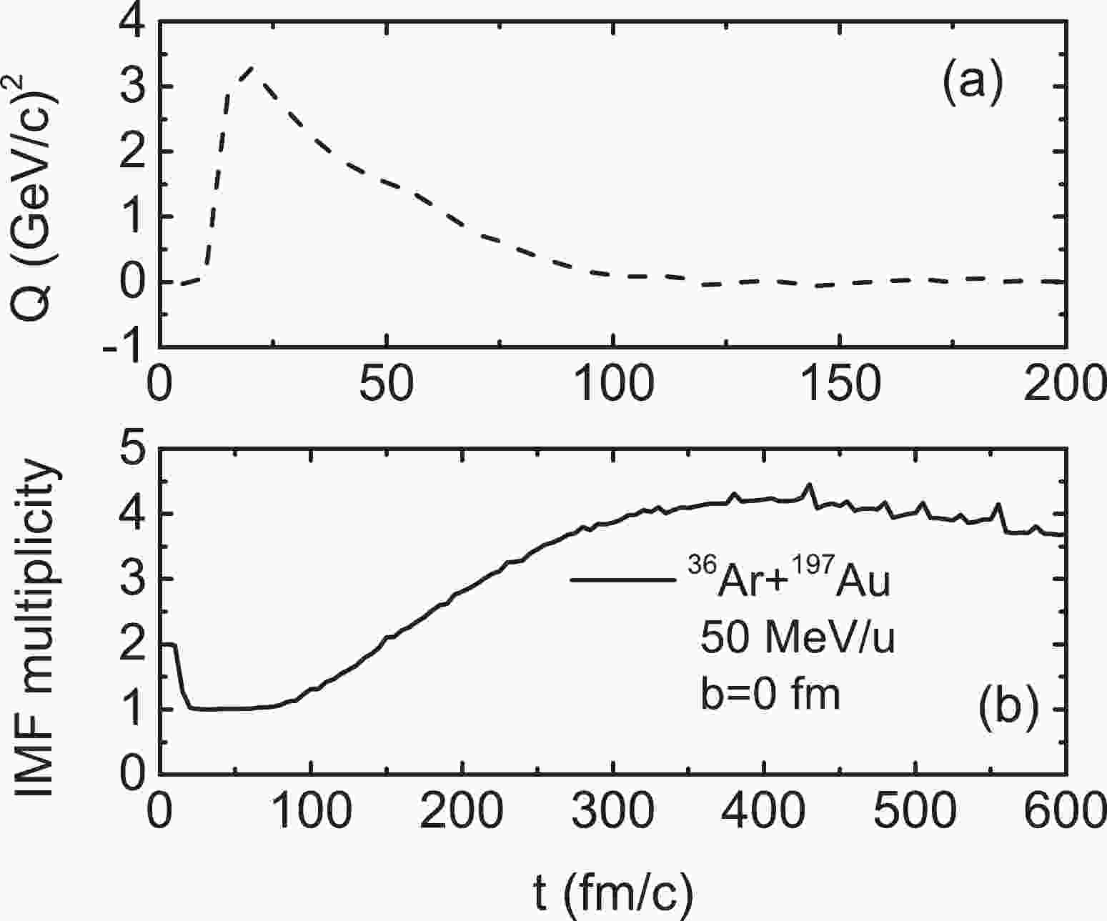
$ \geqslant $ 3 are depicted in Figs. 1(a) and 1(b), respectively. These are calculated for the system$ ^{36} {\rm{Ar}} $ $ + $ $ ^{197} {\rm{Au}} $ at a 50 MeV/u bombarding energy and center collisions. The quadrupole moment of the momentum distribution is determined by
Figure 1. (a) Time evolution of quadrupole momentum for maximum mass cluster and (b) IMF multiplicity for reaction system.
$ Q_{p} = \int(2p_{z}^{2}-p_{x}^{2}-p_{y}^{2}) f({{\mathit{\boldsymbol{r}}}},{{\mathit{\boldsymbol{p}}}},t){\rm d}{{\mathit{\boldsymbol{r}}}}{\rm d}{{\mathit{\boldsymbol{p}}}}. $

(15) The quadrupole moment of the momentum is calculated by all nucleons that belong to the largest cluster in the center of mass of the largest cluster.
It can be observed from Fig. 1(a) that the quadrupole increases rapidly at 10 fm/c. At this moment, the projectile and target are in contact with one another. At approximately 80 fm/c, the quadrupole recovers to zero again. The momentum of nucleons reaches an isotropic distribution at 100 fm/c [24]. Thus, the protons emitted before 100 fm/c comprise pre-equilibrium emission. With the change in the reaction time, the hot nuclei expand and break into primary fragments. The hot nuclei reach the freeze-out stage, and the freeze-out moment can be estimated from the time evolution of the multiplicity of IMFs. It can be observed that the multiplicity of IMFs ends its variation at approximately 400 fm/c. The protons produced after 400 fm/c constitute secondary decay. Therefore, in this study, the protons are divided into four parts: (i) pre-equilibrium emission (PEp), (ii) protons produced in the freeze-out stage (FOp), (iii) secondary decay (SDp), and (iv) PEp+FOp+SDp (TOTAL).
In the following discussion, the focus is on the moderate excitation energy range (6-8 MeV/nucleon). To produce moderate excitation hot nuclei, three beam energies are selected, namely 50, 60, and 70 MeV/u. The reaction system is
$ ^{36} {\rm{Ar}} $ +$ ^{197} {\rm{Au}} $ . At a low excitation energy, evaporation will be the main de-excitation process. The protons originate from the surface of the hot nuclei and not from the freeze-out volume. At a moderate excitation energy (approximately 7 MeV/nucleon), an IMF has a peak value [9], and the hot nuclear system is fully broken. The nucleus breaks into pieces, with the large fragments representing the liquid and the very small ones representing the vapor. The Fermi-gas approach is well justified for this weakly interacting system. More importantly, a nuclear liquid-gas phase transition may occur at a moderate excitation energy [10, 31]. Figure 2 depicts the proton yields of different stages for different excitation energies. It can be observed that the proton multiplicity of pre-equilibrium emission is approximately 4. Most of the protons are produced at freeze-out and via the secondary decay process. The production of secondary decay is approximately 10. Thus, most of the protons are produced by the de-excitation process. Moreover, Fig. 2 indicates that the proton production exhibits a slow increase with an increasing excitation energy.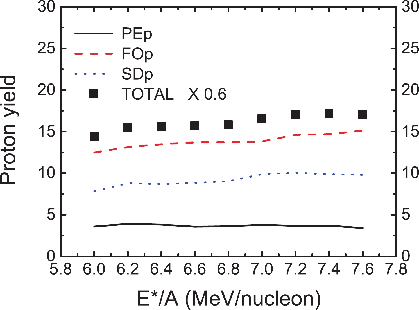
Figure 2. (color online) Proton yield at different stages (PEp, FOp, SDp, and TOTAL) as a function of excitation energy.
In heavy-ion collisions, the hot nuclei will be de-excited by disintegration. The de-excitation process can be light-particle (Z
$ \leqslant $ 2) evaporation or IMF (Z$ \geqslant $ 3) emission. The competition of the two modes determines the de-excitation process. The fragment charge distribution reflects the de-excitation process of the hot nuclei. When the excitation energy is low, the charge distribution has a "U"-shaped characteristic, corresponding to the evaporation event. When the excitation energy is high, the charge distribution has a rapidly decreasing charge distribution, corresponding to the vaporization event [11]. Figure 3 presents the charge distribution as a function of the charge number Z of the fragments. The experimental data are obtained from Ref. [12]. The square symbols indicate the calculated values. The behavior of the calculated charge distribution is generally in agreement with the data. Therefore, our calculation can appropriately describe the de-excitation process of the hot nuclei. The main difference in the calculations compared with the experimental data is the overestimation of the proton yields. However, for the following discussion, the relative proton yields at different stages are more important. The main focus of this study is on the effects of the relative proton yields.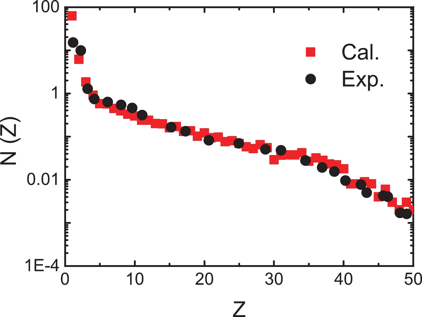
Figure 3. (color online) Charge distribution N(Z) in central
$ ^{197} {\rm{Au}} $ +$ ^{197} {\rm{Au}} $ collisions at 35 MeV/u. The experimental data are obtained from Ref. [12].The freeze-out temperatures are shown in Fig. 4(a). The calculation points are plotted for 0.2-MeV/nucleon-wide bins in excitation energy per nucleon. The MFp versus excitation energy per nucleon is plotted in Fig. 4(b). The proton yield of the secondary decay is approximately 3 times that of the pre-equilibrium emission (see Fig. 2). However, the normalized fluctuations are more easily affected by the pre-equilibrium emission. The secondary decay process is more complex than the pre-equilibrium emission process. Many de-excitation routes are available for secondary decay, and therefore, the competition among the different de-excitation routes increases the fluctuation of the proton production.
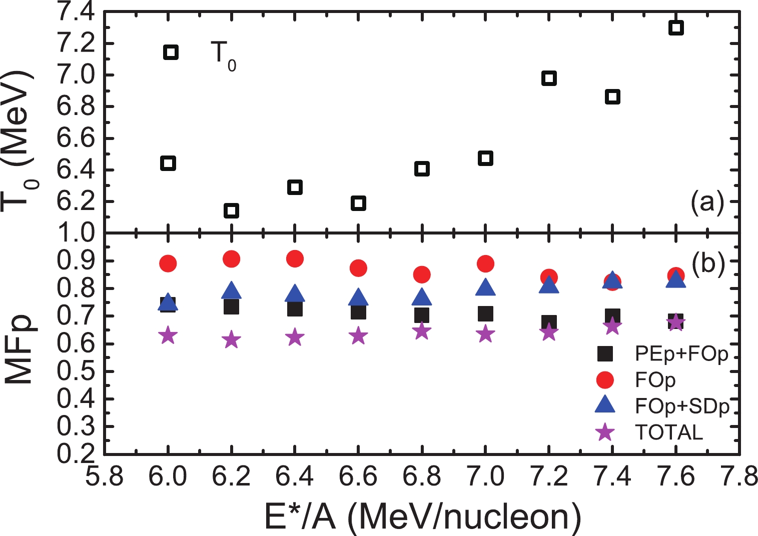
Figure 4. (color online) (a) Freeze-out temperatures and (b) multiplicity fluctuation for proton vs. excitation energy per nucleon
$ E^{*}/A $ .The freeze-out volume versus excitation energy is plotted in Fig. 5. The freeze-out volume can be calculated by four groups of protons (FOp+PEp, FOp, FOp+SDp, and TOTAL). The freeze-out volume calculated by FOp is approximately 2 times that of FOp+PEp. The freeze-out volumes are almost the same between TOTAL and FOp+ PEp. The difference in the freeze-out volume between FOp and FOp+SDp is smaller than that between FOp and FOp+PEp.
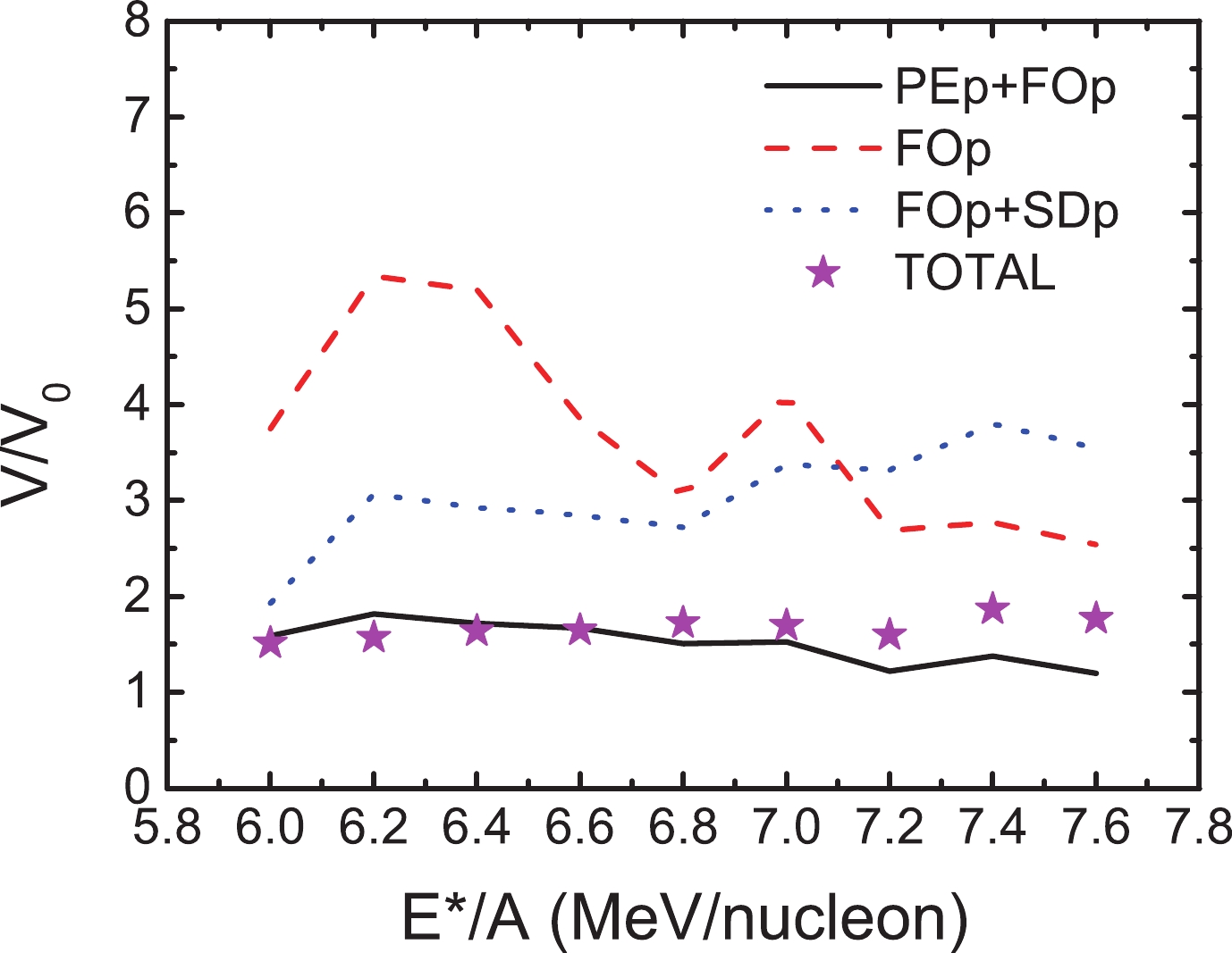
Figure 5. (color online) Freeze-out volume calculated by protons produced at different stages as a function of excitation energy.
The study of the freeze-out volume is helpful for gaining an improved understanding of the multifragmentation process, which may offer the possibility for investigating the nuclear liquid-gas transition. Experimental studies are indespensible to obtain the freeze-out volume and understand the freeze-out concept. However, the particles detected experimentally include the information of pre-equilibrium and secondary decay. The determination of the freeze-out information is affected by the interference of the pre-equilibrium and secondary decay. Therefore, it is necessary to study the effects of pre-equilibrium emission and secondary decay on the determination of the freeze-out information. In this work, the freeze-out volume is studied by the multiplicity fluctuation for a proton. The calculations indicate that pre-equilibrium emission and secondary decay will affect the determination of the freeze-out information. When using the quantum fluctuations of the proton to study the freeze-out volume, the effect of pre-equilibrium emission is more obvious. However, the present results calculated by the IQMD model depend on the model parameters. The use of different model parameters may lead to different results. Therefore, the effects of different model parameters on the determination of the freeze-out volume should be studied in the future.
-
A study on the freeze-out volume from the yields of protons emitted in heavy-ion collisions has been presented in this paper. The study of the freeze-out volume is very important for understanding the multifragmentation process, which opens the possibility for investigating the liquid-gas coexistence region. Experimental studies are indispensable to obtain the freeze-out volume and to understand the freeze-out concept. However, the particles that are detected experimentally include the information of pre-equilibrium emission and secondary decay. The determination of the freeze-out information is affected by the interference of pre-equilibrium and secondary decay.
Owing to the effects of pre-equilibrium emission and secondary decay, the percentage of protons in the freeze-out stage is only approximately 50%. In the de-excitation process, the proton yield produced by secondary decay is approximately 3 times that of pre-equilibrium emission. However, the normalized fluctuations are more easily affected by pre-equilibrium emission because the secondary decay process is more complex. The competition among the different de-excitation routes increases the fluctuation of the proton production. Therefore, when using the multiplicity fluctuation of protons to study the freeze-out volume, more attention should be paid to pre-equilibrium emission.
It should be stressed that the present results are based on specific IQMD model parameters. If different model parameters are used, different results may be obtained. Therefore, these effects should be studied in the future.
The effects of pre-equilibrium emission and secondary decay on the determination of freeze-out volume at intermediate energies
- Received Date: 2020-11-06
- Available Online: 2021-05-15
Abstract: The effects of pre-equilibrium emission and secondary decay on the determination of the freeze-out volume are investigated using the isospin-dependent quantum molecular dynamics model accompanied by the statistical decay model GEMINI. Small-mass projectiles and large-mass targets with central collisions are studied at intermediate energies. It is revealed that the proton yields of pre-equilibrium emission are smaller than those of secondary decay. However, the determination of the freeze-out volume from the proton yields is more easily affected by pre-equilibrium emission. Moreover, the percentage of proton yields in the freeze-out stage is found to be approximately 50%.


 DownLoad: