


 Abstract
 HTML
HTML Reference
 Related
 PDF
PDF


-
The proton represents the unique stable hadron and is one of the elemental constituents of our world. Knowledge of its properties provides an important base to understand the world. In the last twenty years, our knowledge on its structure has been significantly improved; however, some puzzles remain. The electromagnetic form factors (EM FFs) of the proton are two of the most elemental and well-defined non-perturbative quantities reflecting its structures. Precise experimental data sets of the elastic
$ e^{\pm}p $ or$ \mu p $ scattering [1-11] are necessary to extract the EM FFs of the proton. The two-photon-exchange (TPE) effect is key to analyzing and understanding these precise experimental data sets. Since 2003, numerous theoretical dynamical methods and model independent analyses have been proposed and applied to estimate the TPE contribution, such as the hadronic model (HM) method [12-14], GPDs method [15, 16], dispersion relation (DR) method [17-23], perturbative QCD [24, 25], soft collinear effective theory [26], chiral perturbative theory [27], and parametrization method [28-32]. However, this is still far from the accurate estimation of the TPE contribution.To analyze the experimental data sets below a few GeV2, the HM and DR methods are usually employed. In the HM method, the interactions between the photon and the intermediate states (such as nucleon and
$ \Delta(1232) $ ) are constructed to estimate and manifest the TPE amplitude. In the DR method, only the interactions between the photon and the on-shell intermediate states (such as nucleon,$ \Delta(1232) $ and$ \pi N $ continuum) are used to estimate the imaginary part of the TPE amplitude in the physical region. After analytically continuing the imaginary part of the TPE amplitude to the unphysical region and combining it with the asymptotic behavior of the TPE amplitude, the real part of the TPE amplitude is obtained. This means that the DR method only uses the on-shell FFs. It is often argued that this is a considerable advantage of the DR method compared with the HM method, as the latter may include off-shell information. Another advantage of the DR method is the good behavior of the TPE contribution in the Regge limit. The HM method results in unphysical behavior in the Regge limit when excited intermediate states (such as$ \Delta(1232) $ ) are considered. Owing to these advantages, the DR method has recently been widely accepted and applied to analyze the experimental data sets [21-23]. However, this does not mean that the DR method is a perfect and uniquely reliable method. For example, two different DRs are used in Refs. [17-21] and Ref. [22], and the contributions from the meson-exchange effect [33-36] are not included.In this study, we first analyze the analytical structures of the TPE amplitudes in four typical and general toy interactions. Because these interactions are valid at a low energy, we must use them to check low energy behaviors of the TPE amplitudes by the DR method. The detailed comparison and analysis clearly show some important properties on the TPE contributions by the DR and HM methods: (1) the DR and HM methods used in the references must be modified to general forms to correctly include the contributions from the seagull interaction, meson-exchange effect, contact interactions, and off-shell effect; (2) after the modification, the new DRs include a non-trivial term with two singularities; (3) the two methods after the modification yield the exact same results.
-
In the limit
$ m_e\rightarrow0 $ , the amplitude of the elastic$ ep $ scattering with$ C,\;P,\;T $ invariance, Lorentz invariance, and gauge invariance can be written as$ {\cal M}(ep\rightarrow ep) = \sum\limits_{i = 1}^{3} {\cal F}_i{\cal M}_i, $

(1) where all the dynamics are absorbed in the coefficients
$ {\cal F}_i $ and the three independent invariant amplitudes$ {\cal M}_i $ are defined as$ \begin{aligned}[b] {\cal M}_{1} \equiv & M_N[\overline{u}_3\gamma_{\mu}u_1][\overline{u}_4\gamma^{\mu} u_2], \\ {\cal M}_{2} \equiv & [\overline{u}_3({p} \!\!\!/_2+{p} \!\!\!/_4)u_1][\overline{u}_4u_2], \\ {\cal M}_{3} \equiv & M_N[\overline{u}_3\gamma_5\gamma_{\mu} u_1][ \overline{u}_4\gamma_5\gamma^{\mu} u_2]. \end{aligned}$

(2) Here, we have shortly written
$ \overline{u}(p_i,m_i,h_i) $ and$ u(p_i,m_i,h_i) $ as$ \overline{u}_i $ and$ u_i $ ,$ p_{1,2} $ are the momenta of the initial electron and proton,$ p_{3,4} $ are the momenta of the final electron and proton,$ h_i $ are the helicities of the corresponding spinors,$ m_{1,3} = m_e $ and$ m_{2,4} = M_N $ .One can calculate the coefficients
$ {\cal F}_i $ by solving the following algebraic equations:$ \sum\limits_{\rm helicity}{\cal M}{\cal M}^{*}_j = \sum\limits_{i = 1}^{3} \sum\limits_{\rm helicity} {\cal F}_i{\cal M}_i{\cal M}^{*}_j. $

(3) After some simple calculations, the coefficients
$ {\cal F}_i $ can be expressed as$ {\cal F}_{i} = \sum\limits_{j}({\cal D}^{-1})_{ij} \sum\limits_{\rm helicity}{\cal M}{\cal M}^*_j, $

(4) where
${\cal D}_{ij}\equiv\sum\nolimits_{\rm helicity}{\cal M}_{i}{\cal M}^*_{j}$ and are only dependent on the expressions of$ {\cal M}_i $ . In the practical calculation, when$ {\cal F}_i $ exhibits UV divergence, we continue the spinors in$ {\cal M}_i $ to d dimension to maintain the consistency in the full calculation. In the four dimensions, the matrix$ {\cal D}^{-1} $ is expressed as$ {\cal D}^{-1} = \frac{1}{-4M_N^2t(\nu^2-\nu_s^2)^2} \begin{pmatrix} \overline{d}_{11} & \overline{d}_{12} & \overline{d}_{13}\\ \overline{d}_{21} & \overline{d}_{22} & \overline{d}_{23}\\ \overline{d}_{31} & \overline{d}_{32} & \overline{d}_{33} \\ \end{pmatrix}, $

(5) with
$ \begin{aligned}[b] \overline{d}_{11} = & (4M_N^2-t)(\nu^2+\nu_s^2), \\ \overline{d}_{22} = & M_N^2(\nu^2-t(4M_N^2+t)), \\ \overline{d}_{33} = & -t(\nu^2+\nu_s^2),\\ \overline{d}_{12} =& \overline{d}_{21} = -2M_N^2(\nu^2+\nu_s^2),\\ \overline{d}_{13} =& \overline{d}_{31} = 2t(4M_N^2-t)\nu,\\ \overline{d}_{23} = & \overline{d}_{32} = -4M_N^2t\nu, \end{aligned} $

(6) where we define
$ \nu\equiv(p_1+p_3)\cdot(p_2+p_4) $ ,$ t\equiv $ $ (p_1-p_3)^2 $ , and$ \nu_s\equiv\sqrt{-t(4M_N^2-t)} $ .$ {\cal D}^{-1} $ has two kinematic singularities in the unphysical region when$ \nu\rightarrow\pm \nu_s $ . The similar singularities have been discussed in Ref. [21] and are directly neglected when applying the DRs. These kinematic singularities are not physical poles but related with the definition of$ {\cal F}_i $ in the physical region. Usually, such kinematic singularities are cancelled by the corresponding factor in$ \sum{\cal M}{\cal M}^*_j $ , while in some special cases, this cancellation does not happen, and we show this in the following.In the one-photon exchange (OPE) approximation, the amplitude
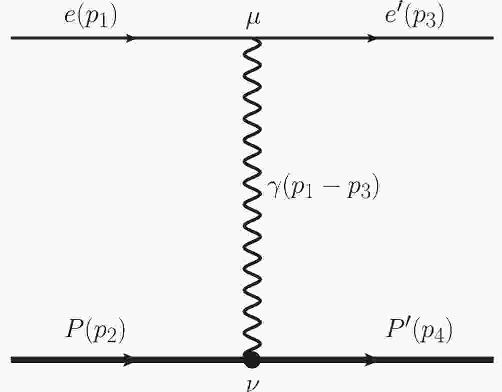
$ {\cal M}^{(1\gamma)} $ corresponding to the Feynman diagram in Fig. 1 can be expressed as follows:
Figure 1. One-photon-exchange diagram for elastic
$ ep $ scattering.$ {\cal M}^{(1\gamma)} = e^2\frac{1}{Q^2}[\overline{u}_3\gamma_{\mu}u_1]\left[\overline{u}_4(F_1\gamma^{\mu}+\frac{F_2}{2M_N}\sigma^{\mu\nu}q_\nu) u_2\right], $

(7) with
$ F_{1,2} $ as the electromagnetic FFs of the proton. The expressions for the corresponding coefficients can be easily obtained, as follows:$ \begin{aligned}[b] {\cal F}_{1}^{(1\gamma)} =& \frac{4\pi\alpha_{e}}{M_NQ^2}(F_1+F_2),\quad {\cal F}_{2}^{(1\gamma)} = -\frac{2\pi\alpha_{e}}{M_NQ^2}F_2,\\ {\cal F}_{3}^{(1\gamma)} =& 0, \end{aligned} $

(8) with
$ \alpha_e = e^2/4\pi $ . The final results$ {\cal F}_i^{(1\gamma)} $ are free from kinematic singularities in$ {\cal D}^{-1} $ when$ {\cal F}_i^{(1\gamma)} $ continues to the complex plane of$ \nu $ . In contrast,$ {\cal F}_i^{(1\gamma)} $ are only dependent on$ Q^2 $ , and their imaginary parts are exactly zero. This means that they obey the once-subtracted DRs on$ \nu $ .When going beyond the OPE approximation, the TPE effect must be considered. In this study, we do not consider TPE contributions from the baryon resonances and
$ \pi N $ continuums, as in principle, their contributions can be handled in a similar manner. In this case, there are four types of dynamical contributions shown in Fig. 2, where$ (a,b) $ are the usual box and crossed-box diagrams, respectively,$ (c) $ is the seagull diagram, and$ (d) $ refers to the meson-exchange effect. For the meson-exchange effect, in principle, one must consider the coupling between mesons and two photons, like the triangle diagram in Fig. 3, which is discussed in Refs. [33-39]. Meanwhile, after the loop integration, the final results can be expressed in a general form as in Fig. 2(d). For simplicity, here, we directly take Fig. 2(d) as an example to discuss the analytical TPE property. The detailed discussions on the magnitudes of the meson-exchange contributions can be found in Refs. [33-39] by the phenomenological models' calculation or the fitting with experimental data sets.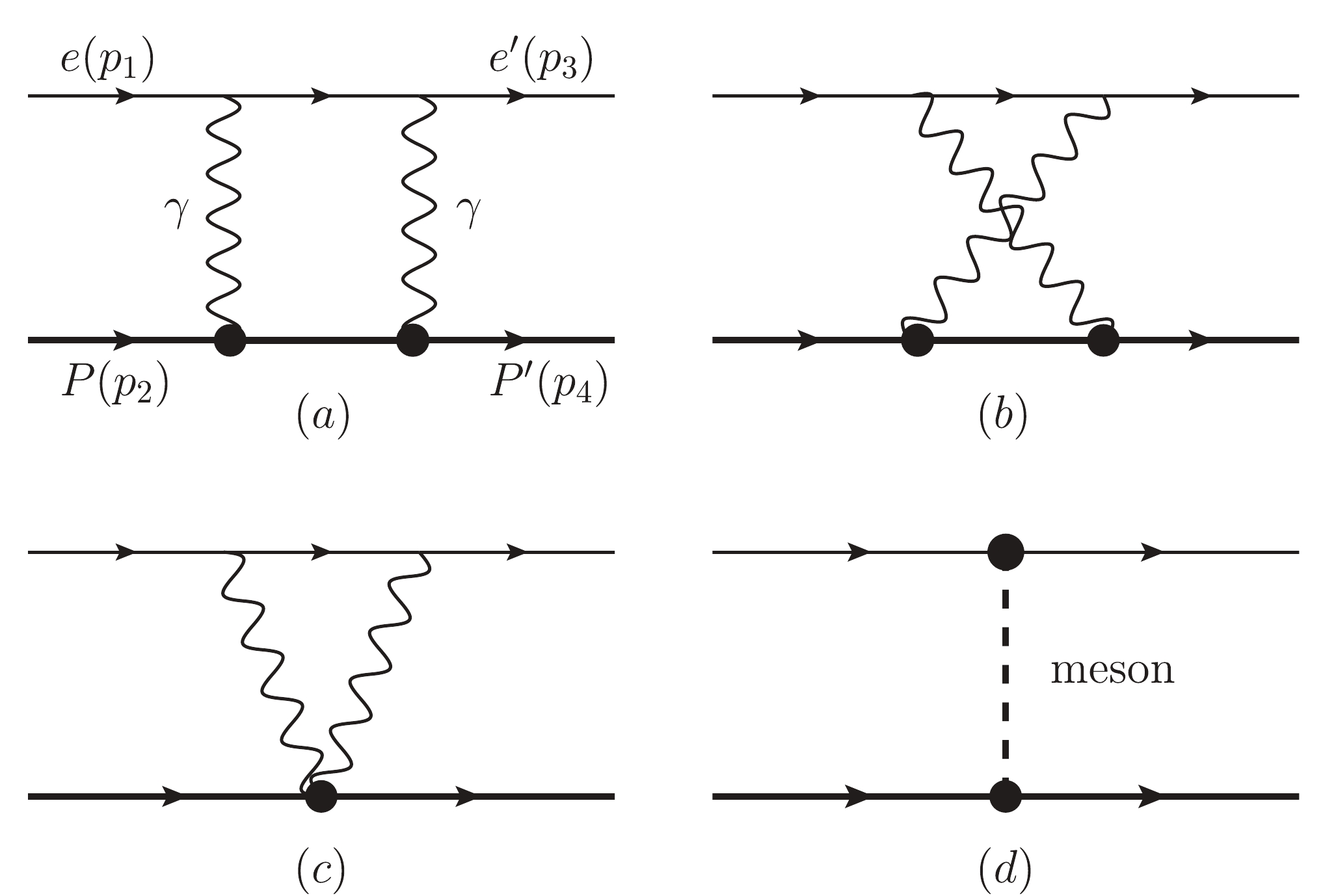
Figure 2. Possible two-photon-exchange effects in elastic
$ ep $ scattering, where only the nucleon intermediate state is considered with the$ (a) $ box,$ (b) $ crossed-box,$ (c) $ seagull, and$ (d) $ meson-exchange diagrams.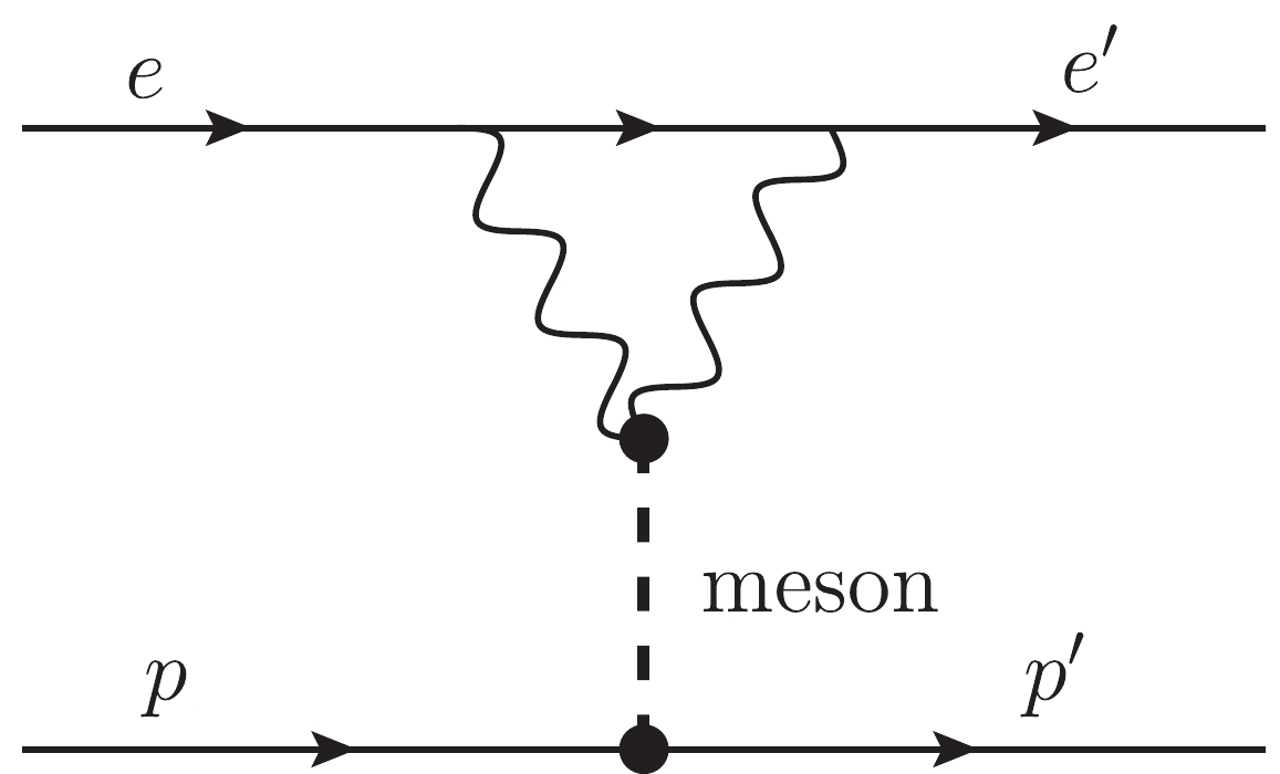
Figure 3. Triangle diagram for meson-exchange contribution via two-photon coupling.
Due to crossing symmetry, one has the following general relations when
$ t<0 $ :$ \begin{aligned}[b] {\cal F}^{(a,c,d)}_{1,2}(t,\nu^+) =& -{\cal F}^{(b,c,d)}_{1,2}(t,-\nu^+),\\ {\cal F}^{(a,c,d)}_{3}(t,\nu^+) =& {\cal F}^{(b,c,d)}_{3}(t,-\nu^+), \end{aligned} $

(9) where
$ \nu^+ = \nu+i0^+ $ , and we use$ {\cal F}^{(a,b,c,d)}_i(t,\nu^+) $ to refer to the coefficients of the TPE amplitudes corresponding to the diagrams$ (a,b,c,d) $ in Fig. 2.In Refs. [17-21] the following DRs are used to estimate the physical TPE contributions:
$ \begin{aligned}[b] {\rm{Re}}[{\cal F}_{1,2}^{ \rm{DR1}}(t,\nu)] =& \frac{2\nu}{\pi} {P}\Bigg[\int_{\nu_{th}}^{\infty}\frac{ {\rm{Im}}[{\cal F}^{(a)}_{1,2}(t,\overline{\nu}^+)]} {\overline{\nu}^2-\nu^2}{\rm d}\overline{\nu}\Bigg], \\ {\rm{Re}}[{\cal F}_{3}^{ \rm{DR1}}(t,\nu)] =& \frac{2}{\pi} {P}\Bigg[\int_{\nu_{th}}^{\infty}\frac{\overline{\nu} {\rm{Im}}[{\cal F}^{(a)}_{3}(t,\overline{\nu}^+)]} {\overline{\nu}^2-\nu^2}{\rm d}\overline{\nu}\Bigg], \end{aligned} $

(10) where the index DR1 refers to the method used in Refs. [17, 21], the operator
$ P $ refers to the principle value integration, and$ \nu_{th} = t $ . In Ref. [22] the DRs are modified as follows:$ \begin{aligned}[b] \rm{Re}[{\cal F}_{1,2}^{ \rm{DR}2}(t,\nu)] =& {\rm{Re}}[{\cal F}_{1,2}^{ \rm{DR}1}(t,\nu)],\\ {\rm{Re}}[{\cal F}_{3}^{ \rm{DR}2}(t,\nu)] =& {\rm{Re}}[{\cal F}_{3}^{ \rm{DR2}}(t,\nu_0)]\\&+\frac{2(\nu^2-\nu_0^2)}{\pi} {P}\Bigg[\int_{\nu_{th}}^{\infty}\frac{\overline{\nu} {\rm{Im}}[{\cal F}^{(a)}_{3}(t,\overline{\nu}^+)]} {(\overline{\nu}^2-\nu^2)(\overline{\nu}^2-\nu_0^2)}{\rm d}\overline{\nu}\Bigg], \end{aligned} $

(11) where the index DR2 refers to the method used in Ref. [22],
$ \nu_0 $ is any real number,$ { \rm{Re}}[{\cal F}_{3}^{ \rm{DR}2}(t,\nu_0)] $ is an unknown function, which can be determined by the experimental data sets at fixed$ \nu_0 $ , and the final result is not dependent on$ \nu_0 $ . To obtain these DRs, the relations in Eq. (9) have been used.These DRs are widely accepted to replace the HM method to estimate TPE contributions and analyze the experimental data sets. While naively, one can easily verify that these DRs do not include the contributions from Fig. 2(c, d), since their imaginary parts are exactly zero when
$ t<0 $ . To understand and solve this problem, in this study, at first we take the following four low energy interactions as examples to show the analytical properties of TPE amplitudes in these interactions:$ \begin{aligned}[b] {\cal L}_{E} \equiv& -e \overline{\psi}_p\gamma^\mu\psi_p A_\mu,\\ {\cal L}_{M} \equiv& -\frac{e\kappa}{4M_N} \overline{\psi}_p\sigma^{\mu\nu}\psi_p F_{\mu\nu},\\ {\cal L}_{S}\equiv& -\frac{2\pi}{M_N^2}(\partial_{\mu}\overline{\psi}_p)(\partial_{\nu}\psi_p) (\alpha_{E1}F^{\mu\rho}{F}^{\nu}_{\rho}+\beta_{M1}\widetilde{F}^{\mu\rho}\widetilde{F}^{\nu}_{\rho}),\\ {\cal L}_{T} \equiv& {\rm i}g_{ \rm{Tpp}}[(\partial_\mu\overline{\psi}_p)\gamma_\nu\psi_p-\overline{\psi}_p\gamma_\nu(\partial_\mu\psi_p) ]\phi^{\mu\nu}\\&+{\rm i}g_{ \rm{Tee}}[(\partial_\mu\overline{\psi}_e)\gamma_\nu\psi_e-\overline{\psi}_e\gamma_\nu(\partial_\mu\psi_e)] \phi^{\mu\nu}, \end{aligned} $

(12) where
$ \psi_{p},A_\mu,\psi_e $ and$ \phi_{\mu\nu} $ refer to the fields of proton, photon, electron, and tensor meson, respectively,$ F_{\mu\nu}\equiv\partial_{\mu}A_\nu-\partial_\nu A_\mu $ and$ \widetilde{F}_{\mu \nu} = \epsilon_{\mu \nu \rho \sigma} F^{\rho \sigma}/2 $ . Similarly to the reason of Fig. 2(d), one can take the direct coupling between the meson and the electrons to discuss the behavior of the TPE amplitude, since the loop integration does not change the analytical property in the region with$ t<0 $ . Furthermore, here we only take$ 2^{++} $ meson as example to show the analytical property, since the contributions from the mesons with other quantum numbers are similar when t is fixed to be negative.By these interactions, the corresponding amplitudes
$ {\cal M}_{E,M}^{(a,b)},\;{\cal M}_{S}^{(c)},\;{\cal M}_{T}^{(d)} $ , and$ {\cal F}_{Xi}^{(y)}(t,\nu) $ are easily obtained, where X refers to$ E,\;M,\;S,\;T $ , and y refers to$ a,\;b,\;c,\;d $ , respectively, and$ {\cal M}_{X}^{(y)} \equiv \sum\limits_{i = 1}^{3} {\cal F}_{Xi}^{(y)}(t,\nu){\cal M}_i. $

(13) -
In the practical calculation, at first we use Eq. (4) to obtain the expressions of the coefficients
$ {\cal F}_{Xi}^{(y)}(t,\nu) $ in d dimensions, and then perform the loop integration with the dimensional regularization. The packages FeynCalc [40, 41] and PackageX [42, 43] are used for the analytical calculation. After the loop integration, we expand$ {\cal F}_{Xi}^{(y)}(t,\nu) $ at$ \nu = \pm \nu_s $ to analyze the kinematic singularities and at$ \nu = $ $ \pm\infty $ to obtain their asymptotic behaviors. The imaginary parts and the discontinuities of$ {\cal F}_{Xi}^{(y)}(t,\nu) $ in the complex plane of$ \nu $ and t are used to analyze the branch cuts.The final analytical results show that the kinematical singularities are cancelled in
$ {\cal L}_{E,S,T} $ cases, but remain in the$ {\cal L}_{M} $ case. The analytical asymptotic behaviors of the coefficients are expressed as follows:$ \begin{aligned}[b] {\rm{Re}}[{\cal F}^{(a)}_{E1}(t,\nu)] &\overset{\nu\rightarrow \infty}{\longrightarrow} -\frac{4\alpha_e^2}{M_Nt}\left[\left(\frac{1}{\widetilde{\epsilon}_{ \rm{IR}}}+\ln\frac{\overline{\mu}^2_{ \rm{IR}}}{-t}\right)\ln {\nu}+c_{1}\right],\\ {\rm{Im}}[{\cal F}^{(a)}_{E1}(t,\nu^+)]& \overset{\nu\rightarrow \infty}{\longrightarrow} \frac{4\pi\alpha_e^2}{M_Nt}\left(\frac{1}{\widetilde{\epsilon}_{ \rm{IR}}}+\ln\frac{\overline{\mu}_{ \rm{IR}}^2}{-t}\right), \\ {\cal F}_{E2,E3}^{(a)}(t,\nu) &\overset{\nu\rightarrow \infty}{\longrightarrow} 0, \end{aligned} $

(14) and
$ \begin{aligned}[b] {\rm{Re}}[{\cal F}^{(a)}_{M1}(t,\nu)] &\overset{\nu\rightarrow \infty}{\longrightarrow} -\frac{\alpha_e^2\kappa^2}{4M_N^3}\Big[\ln^2 \nu-2(1+\ln(-2t))\ln\nu \\&\;\;\;\;\;\;\;\;\; +c_{2}+\frac{3}{4}\frac{1}{\widetilde{\epsilon}_{ \rm{UV}}}\Big],\\ {\rm{Re}}[{\cal F}^{(a)}_{M2}(t,\nu)]& \overset{\nu\rightarrow \infty}{\longrightarrow} \frac{\alpha_e^2\kappa^2}{4M_N^3}c_{3},\\ {\rm{Re}}[{\cal F}^{(a)}_{M3}(t,\nu)]& \overset{\nu\rightarrow \infty}{\longrightarrow} -\frac{\alpha_e^2\kappa^2}{8M_N^3}\Big(5+3\ln\frac{\overline{\mu}_{ \rm{UV}}^2}{-t}+\frac{3}{\widetilde{\epsilon}_{ \rm{UV}}}\Big),\\ {\rm{Im}}[{\cal F}^{(a)}_{M1}(t,\nu^+)]& \overset{\nu\rightarrow \infty}{\longrightarrow} \frac{\pi\alpha_e^2 \kappa^2}{2M_N^3}\Big[\ln \frac{\nu}{-t}-(1+\ln2)\Big], \\ {\rm{Im}}[{\cal F}_{M2,M3}^{(a)}(t,\nu^+)]& \overset{\nu\rightarrow \infty}{\longrightarrow} 0, \end{aligned} $

(15) and
$ \begin{aligned}[b] {\rm{Re}}[{\cal F}^{(c)}_{S2}(t,\nu)] = & -\frac{\alpha_e (\alpha_{E1}+\beta_{E1})}{72M_N^2}\Big(17+12\log\frac{\overline{\mu}_{ \rm{UV}}^2}{-t}+12\frac{1}{\widetilde{\epsilon}_{ \rm{UV}}}\Big)\nu,\\ {\rm{Re}}[{\cal F}^{(d)}_{T1}(t,\nu)] = & \frac{g_{ \rm{Tee}} g_{ \rm{Tpp}}}{M_N(M_T^2-t)}\nu,\\ {\rm{Re}}[{\cal F}^{(d)}_{T3}(t,\nu)] = & \frac{g_{ \rm{Tee}} g_{ \rm{Tpp}}}{2M_{N}(M_T^2-t)}t,\\ {\cal F}_{S1,S3,T2}^{(c,d)}(t,\nu) =& 0, \\ {\rm{Im}}{\cal F}_{S,T}^{(c,d)}(t,\nu) = &0, \end{aligned} $

(16) where
$ \overline{\mu}_{ \rm{IR,UV}} $ are the$ \rm{IR} $ and$ \rm{UV} $ scales,$ c_i $ are some simple functions independent of$ \nu $ , and we do not list them here. Furthermore,$ \frac{1}{\widetilde{\epsilon}_{ \rm{IR,UV}}} = \frac{1}{\epsilon_{ \rm{IR,UV}}}-\gamma_{E}+\ln4\pi. $

The asymptotical behaviors of
$ {\cal F}^{(b)}_{Xi}(t,\nu) $ are obtained easily via Eq. (9).On the branch cuts, the analytical results show: (1) when
$ t<0 $ ,$ {\cal F}_{Xi}^{(a)}(t,\nu) $ has one right hand branch cut in the region$ \nu\subset [\nu_{th},\infty] $ ,$ {\cal F}_{Xi}^{(b)}(t,\nu) $ has one left hand branch cut in the region$ \nu\subset [-\infty,-\nu_{th}] $ , and$ {\cal F}_{Xi}^{(c,d)}(t,\nu) $ has no branch cut. There properties are shown in Fig. 4, and are natural due to the unitarity usually argued in the references. (2) when$ t>0 $ ,$ {\cal F}_{Xi}^{(a,b,c,d)}(t,\nu) $ has an additional branch cut at a real axis of t, and this discontinuity on t results in the nonzero imaginary parts of$ {\cal F}_{Xi}^{(a,b,c,d)}(t,\nu) $ . This is likewise natural, since when$ t>0 $ the coefficients$ {\cal F}_{Xi}^{(y)}(t,\nu) $ are related with the TPE contributions in$ e^+e^-\rightarrow p\overline{p} $ .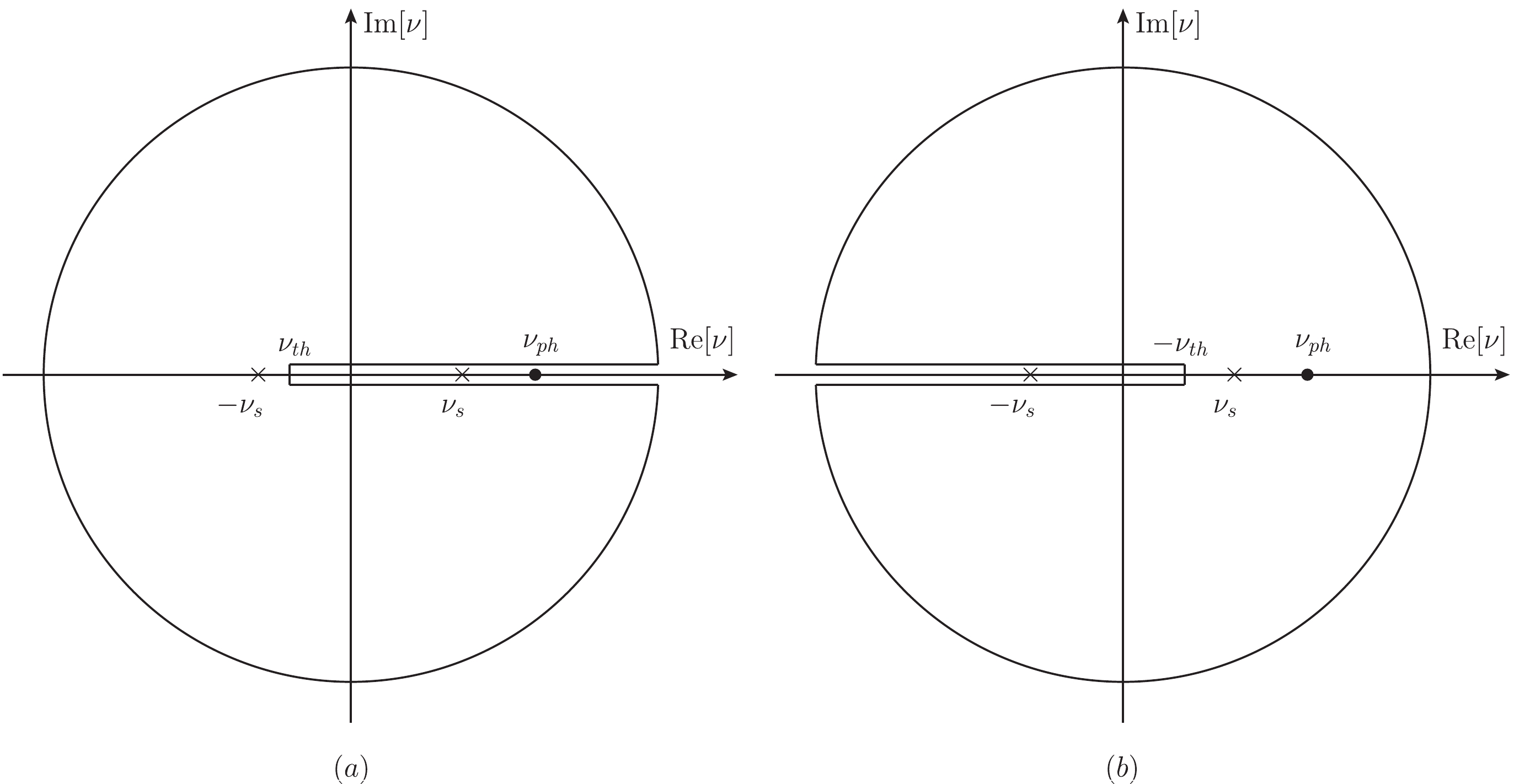
Figure 4. Branch cuts of
$ {\cal F}_i^{(a,b)}(Q^2,\nu) $ in complex plane of$ \nu $ at fixed negative t. (a) is for$ {\cal F}_i^{(a)}(t,\nu) $ and (b) is for$ {\cal F}_i^{(b)}(t,\nu) $ where the physical$ \nu_{\rm ph} $ , and possible kinematic singularities are marked.The summary of analytical properties is presented in Table 1. By combing these analytical properties and Eq. (9), it is easy to verify that
$ {\cal F}_{Ei}^{(a+b)}(t,\nu) $ satisfy Eq. (10) and$ {\cal F}_{Mi}^{(a+b)}(t,\nu)-{\cal F}_{Mi, \rm{ks}}^{(a+b)}(t,\nu) $ satisfy Eq. (11) when$ t<0 $ , where$ {\cal F}_{Mi, \rm{ks}}^{(a+b)}(t,\nu) $ include two kinematic singularities and are expressed asasymptotical behavior of
Re part at$ \nu\rightarrow\infty $ 

asymptotical behavior of
Im part at$ \nu\rightarrow\infty $ 

kinematical
singularitiesbranch cut UV IR $ {\cal F}_{E1}^{(a)} $ 

$ x_1\ln\nu $ 

$ -\pi x_1 $ 

− [ $ \nu_{th},\infty $ ]

− Yes $ {\cal F}_{E2}^{(a)} $ 

0 0 − [ $ \nu_{th},\infty $ ]

− − $ {\cal F}_{E3}^{(a)} $ 

0 0 − [ $ \nu_{th},\infty $ ]

− − $ {\cal F}_{M1}^{(a)} $ 

$ x_2\ln^2\nu $ 

$ -2\pi x_2\ln\nu $ 

Yes [ $ \nu_{th},\infty $ ]

Yes − $ {\cal F}_{M2}^{(a)} $ 

$ x_3 $ 

0 Yes [ $ \nu_{th},\infty $ ]

− − $ {\cal F}_{M3}^{(a)} $ 

$ x_4 $ 

0 Yes [ $ \nu_{th},\infty $ ]

Yes − $ {\cal F}_{S1}^{(c)} $ 

0 0 − − − − $ {\cal F}_{S2}^{(c)} $ 

$ x_5\nu $ 

0 − − Yes − $ {\cal F}_{S3}^{(c)} $ 

0 0 − − − − $ {\cal F}_{T1}^{(d)} $ 

$ x_6\nu $ 

0 − − − − $ {\cal F}_{T2}^{(d)} $ 

0 0 − − − − $ {\cal F}_{T3}^{(d)} $ 

$ x_7 $ 

0 − − − − Table 1. Analytical properties of coefficients
$ {\cal F}_{Xi}^{(y)}(t,\nu) $ at fixed negative t, where$ x_i $ are constants whose expressions are obtained from Eqs. (14)-(16), and the symbol - indicates that there is no such contributions. Analytical properties of$ {\cal F}^{(b)}_{Xi}(t,\nu) $ are not listed, as they can be obtained easily via Eq. (9).$ {\cal F}_{Mi, \rm{ks}}^{(a+b)}(t,\nu) = \frac{A^{(a+b)}_i(\nu,t)}{(\nu^2-\nu_s^2)^2}, $

(17) with
$ A^{(a+b)}_i(\nu,t) $ being three polynomials of$ \nu $ and t, their manifest expressions are slightly long and are listed in the appendix. Furthermore,$ {\cal F}_{M3}^{(a+b)}(t,\nu) $ includes an UV divergence, which means that the single interaction$ {\cal L}_{M} $ is not consistent, and the corresponding contact interactions must be considered to absorb UV divergence. This means that the usual HM method must be modified to include the contact interactions. Therefore, DR2 is used in Ref. [22] to replace DR1.We find that if the two photons are assigned some virtual masses (different or same) in the Feynman gauge, the terms
$ {\cal F}_{Mi, \rm{ks}}^{(a+b)}(t,\nu) $ are not changed. This means that the contributions with the kinematical singularities are exactly cancelled when one replaces the vertex$ \Gamma_{M}^{\mu}(k) $ (from$ {\cal L}_M $ ) by$ \Gamma_{M}^{\mu}(k)F(k^2) $ with$ F(k^2) $ being a monopole like FF, as follows:$ F(k) = \sum\limits_{j}\frac{d_j}{(k^2-\Lambda^2_j)^{n_j}}, $

(18) where k is the momentum of the incoming photon,
$ n_j $ are some natural numbers, and$ d_j,\Lambda_j $ are some real parameters. This cancellation is due to the following simple relation and its generalization.$ \frac{B}{(k^2-z_1^2)(k^2-z_2^2)} = \frac{1}{z_1^2-z_2^2}\left[\frac{B}{k^2-z_1^2}-\frac{B}{k^2-z_2^2}\right]. $

Because
$ {\cal F}_{Mi, \rm{ks}}^{(a+b)}(t,\nu) $ are not dependent on the parameters$ z_j $ , the two contributions with the kinematical singularities are canceled. This property indicates that the coefficients$ {\cal F}_{i}^{(a+b)}(t,\nu) $ in the usual HM method with a monopole like FFs as inputs are free from any kinematical singularities. This explains the numerical property of Fig. 19 in Ref. [22], where the difference between the DR and HM methods with FFs are presented. The important point is that this does not mean that the kinematical singularities are canceled certainly in any cases.Another important property is that
$ {\rm{Im}}[{\cal F}_{Si}^{(c)}(t,\nu)] $ and$ {\rm{Im}}[{\cal F}_{Ti}^{(d)}(t,\nu)] $ are exactly zero, whereas$ { \rm{Re}}[{\cal F}_{S2}^{(c)}(t,\nu)] $ and$ {\rm{Re}}[{\cal F}_{T1,T3}^{(d)}(t,\nu)] $ are not zero and satisfy twice-subtracted and once-subtracted DRs, respectively. Similarly, there is an UV divergence in$ {\rm{Re}}[{\cal F}_{S2}^{(c)}] $ , which means that the contact interactions must be included to absorb UV divergence. These properties are general when extending the interactions to general forms by including more derivatives. Similarly, when the mesons with other J are considered, the results are still polynomial functions on$ \nu $ . After combing these contributions, one can see that the contributions from the seagull interaction, the meson-exchange, and contact interaction can be expressed as$ \begin{aligned}[b] {\cal F}_{1,2}^{(c+d)}(t,\nu) =& \sum\limits_{j = 0}c_{1j,2j}(t)\nu^{2j+1},\\ {\cal F}_{3}^{(c+d)}(t,\nu) =& \sum\limits_{j = 0}c_{3j}(t)\nu^{2j}, \end{aligned} $

(19) where the properties Eq. (9) have been used. At first glance, these results are unphysical at high energy and are directly neglected in the usual calculation. However, their physical meaning is seen clearly when one continues the results to the physical region of
$ e^+e^-\rightarrow p\overline{p} $ , where the variable$ \nu $ corresponds to$ -\nu_s\cos\theta_p $ with$ \theta_p $ as the angle of the final proton's three momentum in the center of mass frame. The physical regions of$ \nu,t $ in$ ep\rightarrow ep $ and$ e^+e^-\rightarrow p\overline{p} $ indicate that the contributions Eq. (19) converge in the regions$ \nu\rightarrow \infty $ and$ |\nu|<\nu_s $ . They are given as follows:$ \begin{aligned}[b] \sum\limits_{j = 0}c_{1j,2j}(t)\nu^{2j+1} =& \sum\limits_{j = 1}\frac{g_{1j,2j}(t)\nu}{(\nu^2-\nu_s^2)^j}\approx \frac{g_{11,21}(t)\nu}{\nu^2-\nu_s^2},\\ \sum\limits_{j = 0}c_{3j}(t)\nu^{2j} =& \sum\limits_{j = 0}\frac{g_{3j}(t)}{(\nu^2-\nu_s^2)^j}\approx g_{30}(t), \end{aligned} $

(20) where
$ g_{ij}(t) $ are unknown functions and only the leading contributions are kept, as$ \nu^2-\nu_s^2 $ increases quickly when$ \nu $ increases at fixed t. The interesting property is that these contributions are the same with Eq. (17) in the leading order.Finally, one obtains the following DRs in the leading order of
$ M_N^4/(\nu^2-\nu_s^2) $ :$ \begin{aligned}[b] {\rm{Re}}[{\cal F}_{1,2}^{ \rm{DR3}}(t,\nu)] =& \frac{f_{1,2}(t) \nu}{\nu^2-\nu_s^2}+\frac{2\nu}{\pi} {P}\Bigg[\int_{\nu_{th}}^{\infty}\frac{ {\rm{Im}}[{\cal F}^{(a)}_{1,2}(t,\overline{\nu}^+)]} {\overline{\nu}^2-\nu^2}{\rm d}\overline{\nu}\Bigg],\\ {\rm{Re}}[{\cal F}_{3}^{ \rm{DR3}}(t,\nu)] =& {\rm{Re}}[{\cal F}_{3}^{ \rm{DR3}}(t,\nu_0)]\\&+\frac{2(\nu^2-\nu_0^2)}{\pi} {P}\Bigg[\int_{\nu_{th}}^{\infty}\frac{\overline{\nu} {\rm{Im}}[{\cal F}^{(a)}_{3}(t,\overline{\nu}^+)]} {(\overline{\nu}^2-\nu^2)(\overline{\nu}^2-\nu_0^2)}{\rm d}\overline{\nu}\Bigg], \end{aligned} $

(21) where we use
$ f_{i}(t) $ to refer to the unknown functions. Eqs. (19)-(21) indicate the following exact relations between DR3 and the modified HM method:$ \begin{aligned}[b] {\cal F}^{ \rm{DR3}}_{1,2}(t,\nu) = & \Bigg[{\cal F}^{(a+b)}_{1,2}(t,\nu)+\sum\limits_{j = 0}h_{1j,2j}(t)\nu^{2j+1}\Bigg]_{ \rm{Ana+LO}},\\ {\cal F}^{ \rm{DR3}}_{3}(t,\nu) =& \Bigg[{\cal F}^{(a+b)}_{3}(t,\nu)+\sum\limits_{j = 0}h_{3j}(t)\nu^{2j}\Bigg]_{ \rm{Ana+LO}}, \end{aligned} $

(22) where the subindex
$ \rm{Ana+LO} $ refers to do analytical continuation and maintains the leading order contribution,$ h_{ij}(t) $ includes the contributions from the seagull interaction, the meson-exchange effect, and the contact interactions.Indeed, the contributions due to the off-shell effects in
$ (a+b) $ can also be expressed by$ h_{ij}(t) $ . This is understood in a direct physical manner. In the DR method, only the on-shell vertex of$ \gamma^*NN $ is used to estimate the imaginary parts of the coefficients, and the real parts are obtained by the DRs. In the HM method, if the off-shell vertex is used, one can separate the vertex into two parts as$ \Gamma_\mu^{ \rm{off-shell}}(p_{i,f}^2,k^2) = \Gamma_\mu^{ \rm{on-shell}}(k^2)+\Delta \Gamma_{\mu}(p_{i,f}^2-M_N^2,k^2), $

(23) where
$ p_i,p_f $ are the momenta of the initial and final proton in the vertex, respectively,$ \Delta \Gamma(p_{i,f}^2-M_N^2,k^2) $ is a polynomial function on$ p_i^2-M_N^2 $ or$ p_f^2-M_N^2 $ when no additional phenomenological poles on$ p_i^2 $ and$ p_f^2 $ are introduced in the vertex. Then, the TPE amplitude can be separated into two parts: one only includes the on-shell information, and another includes the off-shell effect. Naively, the first one is obtained by the DR1 method. The second one has a global factor like$ p_i^2-M_N^2 $ or$ p_f^2-M_N^2 $ in the numerator. This factor cancels the denominator of the nucleon's propagator, and the final result after the loop integration is similar to the contribution from the seagull interaction. This means that the contributions due to the off-shell effect can be expressed by some polynomials on$ \nu $ like the contributions from the seagull interaction, the meson-exchange effect, and contact interactions. This property clearly indicates the physical meaning of$ h_{ij}(t) $ . They include all the contributions due to the seagull interaction, the meson-exchange effect, the contact interactions, and the off-shell effect. -
In summary, detailed analysis based on four typical and general interactions clearly shows that the usual DR and HM methods must be modified to general forms. After the modifications, the two methods yield exactly the same results, which automatically include contributions from the seagull interaction, the meson-exchange effect, contact interactions, and the off-shell effect in a correct manner. The physical reason why they are exactly the same is likewise discussed. The expressions in the modified DR and HM methods in the leading order are expressed by Eq. (21) and Eq. (22). One must use them to analyze the corresponding experimental data sets and extract physical quantities. The novel DRs have two additional parameters, which makes it more difficult to extract the full TPE contributions from the experimental data sets. In this study, our aim is to show the exact relations between the HM method and DR method; therefore we do not perform fitting with the experimental data sets.
-
H.Q.Z. thanks Shin Nan Yang for his helpful discussion in the TPE effect and thanks Hiren H. Pate for his kind help in the use of PackageX. He acknowledges the support of the National Center for Theoretical Science of the National Science Council of the Republic of China for his visits in July, 2019. He also greatly appreciates the warm hospitality extended to him by the Physics Department of the National Taiwan University during the visits.
-
In this appendix, the expressions for
$ A^{(a,b)}_i(\nu,t) $ are presented.The expressions for
$ A^{(a,b)}_{i} $ are slightly complex, and for simplicity, we separate them into two parts : the first part$ A^{ {\rm{I}}(a,b)}_{i} $ arises from the finite parts of the pure loop integrations and the finite trace of Dirac matrix, the second part$ A^{ {\rm{II}}(a,b)}_{i} $ arises from the divergent parts of the pure loop integrations and the trace of Dirac matrix with factor$ (d-4) $ . Finally, we have the following expressions:$\tag{A1} \begin{aligned}[b] A^{ {\rm{I}}(a)}_{1} =& -\alpha_e^2 \kappa^2\frac{(4M_N^2-t)(2\nu-3t)}{8M_N^3}(\nu^2-\nu_s^2),\\ A^{ {\rm{I}}(a)}_{2} =& \alpha_e^2 \kappa^2\frac{2\nu-3t}{4M_N}(\nu^2-\nu_s^2),\\ A^{ {\rm{I}}(a)}_{3} = & -\alpha_e^2 \kappa^2\frac{(8M_N^2-2t+3\nu)t}{8M_N^3}(\nu^2-\nu_s^2), \end{aligned} $

and
$\tag{A2} \begin{aligned}[b] A^{ {\rm{II}}(a)}_{1} =& -\alpha_e^2 \kappa^2\frac{4M_N^2-t}{8M_N^3} \Big[2t(4M_N^2-t)(7t+10\nu)\\&-(11t+4\nu)(\nu^2-\nu_s^2) \Big],\\ A^{ {\rm{II}}(a)}_{2} = & \alpha_e^2 \kappa^2\frac{1}{4M_N} \Big[2t(4M_N^2-t)(7t+10\nu)\\&-(11t+4\nu)(\nu^2-\nu_s^2) \Big],\\ A^{ {\rm{II}}(a)}_{3} =& \alpha_e^2 \kappa^2\frac{t}{4M_N^3} \Big[-t(4M_N^2-t)(40M_N^2-10t-7\nu)\\&+(28M_N^2-7t-2\nu)(\nu^2-\nu_s^2) \Big].\\ \end{aligned} $

The corresponding expressions for
$ A^{(b)}_{i} $ can be obtained by the relations between$ {\cal F}_i^{(a)}(t,\nu) $ and$ {\cal F}_i^{(b)}(t,\nu) $ . These expressions are also checked by the numerical calculation.
Exact relations for two-photon-exchange effect in elastic ep scattering by dispersion relation and hadronic model
- Received Date: 2021-01-14
- Available Online: 2021-07-15
Abstract: The two-photon-exchange (TPE) effect plays a key role in extracting the form factors (FFs) of the proton. In this work, we discuss several exact properties of the TPE effect in the elastic


 DownLoad: