


 Abstract
 HTML
HTML Reference
 Related
 PDF
PDF


-
Astrophysical observational data substantially support the speculations about the cosmic expansion of the universe, and reveal some mysterious components present in the universe [1]. The basis of this result is actually the collaboration of the Friedman-Robertson-Walker-type geometry with cosmology, as well as currently available astronomical data. Therefore, precisely, considering the current available information on astronomical data, the only result that can be presently determined is that the pressureless Einstein-de Sitter model is not favored by the scrutiny. In general, the theoretical reasons for the expansion of the universe are described in two approaches. The first is based on altering the contents of the universe, realized by applying the dark energy sector, initiating from a canonical sector field or both as a unit model, and paving the path for further complex configurations [2, 3]. The second approach is based on modifying the gravitational sector [4-8]. Considering the issues regarding physical interpretations, one can modify it as a whole or partially from one way to another; however the number of extra degrees of freedom [9] is actually an important aspect. Therefore, both approaches described above can be used together or in a framework with the combination of the gravitational and non-gravitational sectors.
The basis for modifying theories of gravity is conventionally the generalization of the Einstein-Hilbert action in the general relativity (GR) theory, such that these theories are developed with the curvature concept of gravity. However, an unmatched and compulsive modification of gravity was observed when the action of GR identical to the geometric formulation of GR based on torsion, was extended. Einstein himself developed an equivalent GR theory, which he remarkably referred to as "TEGR" (Teleparallel Equivalent of General Relativity). The TEGR formulation of gravity is elucidated by the torsion-dependent Weitzenbock connection [10-12], instead of the curvature deployed Levi-Civita connection. Therefore, the Lagrangian elaborated by the torsion scalar T, originates from the contraction of the torsion tensor, analogous to the Einstein-Hilbert Lagrangian, which originates from the Riemanian (curvature) tensor. Hence, rather than modifying GR, TEGR can be generalized, and
$ f(T) $ simply developed by extending the Lagrangian with a discretionary torsion function [13-15], in addition to the torsion T. It is more attractive to know that TEGR is equalent to GR in terms of its equations; however,$ f(T) $ is divergent to$ f(R) $ , such that they generate dissimilar modifications. Different generalizations of the$ f(T) $ gravity theory have also been proposed in the literature. One of such proposals introduced a novel Lagrangian scalar$ f(T,B) $ , which involves a boundary term B related to the divergence of the torsion tensor [16-21]. This theory becomes equivalent to the$ f(R) $ gravity for the selected special form$ f(T + B) $ because the Einstein-Hilbert action Lagrangian is dynamically equivalent to this argument choice. An extended version of$ f(T) $ gravity is the coupling of torsion T with the trace$ {\cal{T}} $ of the energy momentum tensor (EMT) [22], which results in$ f(T,{\cal{T}}) $ , a new modification of gravity that is dissimilar to all other forms of torsion and curvature-dependent gravities. This modified gravity takes its inspiration from the modified$ f(R,{\cal{T}}) $ gravity [23-25], where instead of having the Ricci scalar R coupled with the trace of the EMT$ {\cal{T}} $ , the torsion scalar T is coupled with$ {\cal{T}} $ . In$ f(T,{\cal{T}}) $ , various cosmic aspects have been explored, including the reconstruction of cosmic models, their stability, thermodynamic aspects, late time aspects, and dark energy models [26-30].Being at the extremity, in the formation of an ordinary star, compact stars play a crucial role in describing the configuration of highly-condensed substances in intense situations. In astrophysics, some of the highly dense compact objects that have strong magnetic fields, such as pulsars and other spinning stars, are considered remarkable discoveries. Owing to the omission of the Catholic church's elucidation of these dense bodies, it is confined that these objects are actually the combinations of subatomic particles such as baryons, leptons, and mesons, except strange quark matter. Nevertheless, in astrophysics, the basic objective is to discover the geometry and configurations of intramural and inshore substances of compact stellar objects. The study on the formation of compact stars, as well as the gravitational collapse phenomenon, is regarded as one of the most fascinating topics in modern cosmology and astronomy. In 1916, Carl Schwarzschild presented the exact solution on the interior of symmetric stars spherically by adopting the uniform density-based matter profile [31]. In 1939, Oppenheimer and Snyder [32] contributed to the exploration of the gravitational collapse with homogeneity-based dust sphere. In the literature [33-37], several static analytic models representing the relativistic stars have been constructed by introducing bulk viscous effects, anisotropic pressures, charge, multilayered fluids, and equations of state. Recently, compact stars have been discussed as major trends in different amended theories of gravity, such as
$ f(G) $ gravity [38],$ f(R) $ gravity [39],$ f(R,{\cal{T}}) $ gravity [40-44],$ f(T,{\cal{T}}) $ gravity [45], and other alternative theories of gravity. In [46], Rahaman et al. discussed the possibility of applying the Krori and Barua (KB) model [47] to describe ultra-compact objects, such as strange stars. In their study, they analyzed the mathematical formulation of strange star models. Shahzad and Abbas [48] used the KB insatz in the static and spherically symmetric geometry to discuss quintessence compact stars models in Rastall gravity. Sharif and Majid [49] discussed the extension of isotropic spherically symmetric solutions to anisotropic domains via minimal geometric deformations in the context of the self-interacting Brans-Dicke theory. They employed the anisotropic KB solution and extended the Durgapal-Fuloria solution in this study, based on the MGD approach. The KB solution is also discussed in$ f(R,T) $ , based on the MIT bag model, which results in singularity-free and physically acceptable solutions [50]. In recent work, Roupas and Nashed [51] modeled anisotropic neutron stars working in the KB ansatz without preassuming an equation of state (EOS). It is determined that stability requirements yield the compactness limit to be$ 2GM/Rc^2<0.71 $ .Here, we study the physically admissible results for anisotropic compact objects in a non-minimally-coupled torsion-based theory,
$ f(T,{\cal{T}}) $ gravity. In the$ f(T,{\cal{T}}) $ gravity, compact stellar configuration has been presented for isotropic matter fluid distribution, which corresponds to embedding the class I model for LMC X-4 and Vela X-1 compact stars using a specific linear function$ f(T, {\cal{T}}) = \alpha T(r)+\beta {\cal{T}} (r) + \Phi $ , where α and β represent any arbitrary constant, and Φ represents the cosmological constant [45]. In [52], Salako et al. discussed strange star models via anisotropic fluid distribution in the$ f(T,{\cal{T}} $ ) gravity. They adopted the diagonal tetrad matrix and explored the role of the strange quark star model. In previous studies [52, 53], field equations are obtained by employing the diagonal matrix choice of the tetrad field, which is considered an inappropriate choice in torsion-dependent gravity theories, as it imposes some limitations on the modification of the gravity theory [54, 55] by restricting the functional form of the theory to the linear one. To address these limitations by avoiding the bad choice, we adopted corrected off-diagonal tetrad and a more generic modification of the$ f(T, {\cal{T}}) $ gravity theory, i.e.,$ f(T,{\cal{T}}) = \alpha T^{n}(r)+ $ $ \beta {\cal{T}} (r)+\phi $ . We elucidated the linear and non-linear modifications by selecting$ n = 1 $ and non-linear modification results by choosing$ n = 2 $ , respectively. Therefore, the results obtained in our study are more generic, and adopt the correct formalism of theoretical physics. We consider the anisotropic KB solution, and discuss the existence of anisotropic compact star candidates. The objective of this paper is to determine the constraints on the$ f(T,{\cal{T}}) $ model, and the parameters of the theory, if the compact star solutions exist in this model. We selected the parameters based on the observational data of various compact stars, such as$ PSR J1416- $ $ 2230 $ ,$ 4U 1608-52 $ ,$ Cen X-3 $ ,$ EXO 1785-248 $ , and$ SMC X-1 $ .This paper is organized as follows. In Sec. II, we discuss the basics of the
$ f(T,{\cal{T}}) $ theory adopted in this study. Here, we generalize the solutions of field equations by utilizing the KB metric. In Sec. III, we evaluate the values of unknown parameters using matching conditions. In Sec. IV, we reveal the anisotropic characteristics of the compact stars by discussing the behaviors of density, pressures, gradients, and anisotropy. In Sec. IV.E, we discuss the realistic behavior of matter by considering its energy conditions. In Sec. V, we determine the physical viability and acceptability of the compact stars by discussing the behavior of EOS, casuality conditions, equilibrium, mass function, compactness, and redshift function. Throughout this study, we monitor the data of compact stars,$ PSR J1416-2230 $ ,$ 4U 1608-52 $ ,$ Cen X-3 $ ,$ EXO 1785-248 $ and$ SMC X-1 $ , already discussed in literature. Finally, in Sec. VI, we conclude our study based on analytical and graphical solutions. -
As is well-known, TEGR is an adjoining alteration in GR; however
$ f(T) $ is significantly differs from TEGR when it is generalized in terms of the torsion T function. Hence,$ f(T) $ describes the gravity in a very dissimilar way from the curvature based$ f(R) $ gravity. A parallel form of$ f(R,{\cal{T}}) $ gravity is$ f(T,{\cal{T}}) $ gravity, whose Lagrangian is defined by the action as [22]:$ s = \int {\rm d}x^{4} e\left\{ \frac{1}{2k^{2}} f(T,{\cal{T}})+{\cal{L}}_{(M)}\right\}, $

(1) where
$ e = {\rm det}\left( e_{\mu}^{A}\right) = \sqrt{-g} $ and$ k^{2} = 8\pi G = 1 $ . In addition,$ {\cal{L}}_{(M)} $ represents the function, which shows that the Lagrangian density and f are torsion-trace ($ T,{\cal{T}} $ )-dependent functions. The equations of motion are extracted from the variation of Eq. (1) relative to tertrad field:$ \begin{aligned}[b] &e_{i} {}^{\gamma}S_{\gamma}{}^{\mu\eta}f_{TT}\partial_{\mu}T+e_{i} {}^{\gamma}S_{\gamma}{}^{\mu\eta}f_{T{\cal{T}}}\partial_{\mu}{\cal{T}}+e^{-1}\partial_{\mu}(ee_{i}{}^{\gamma} S_{\gamma}{}^{\mu\eta})f_{T}\\ &- e_{\eta}{}^{i}T^{\gamma}{}_{\mu i}S_{\gamma}{}^{\eta\mu}f_{T}-\frac{1}{4}e_{i}{}^{\eta}f+f_{T}\omega^{\gamma}{}_{\eta\mu}S_{\gamma}{}^{\eta\mu} -\frac{f_{\cal{T}}}{2}(e_{\eta}{}^{i}T_{i}{}^{\eta}+p_t e_{\eta}{}^{i})\\ = &-4\pi e_{\eta}{}^{i}T_{i}{}^{\eta}, \end{aligned} $

(2) where
$ T_{i}^ {\nu} $ denotes the EMT,$ f_{T} = \dfrac{\partial f}{\partial T} $ ,$ f_{TT} = \dfrac{\partial^{2} f}{\partial T^2} $ ,$ f_{\cal{T}} = \dfrac{\partial f}{\partial {\cal{T}}} $ , and$ f_{T{\cal{T}}} = \dfrac{\partial^{2} f}{\partial T\partial {\cal{T}}} $ . The spin connection$ \omega^{\gamma}{}_{\eta\mu} $ is considered to be zero in the begining. Core components used in Eq. (2), such as torsion contorsion and super-potential, are expressed as:$ T^{\lambda}_{\mu\eta} = e_{\vartheta}{}^{\lambda}(\partial_{\mu}e^\vartheta{}_\eta-\partial_{\eta}e^\vartheta{}_{\mu}), $

(3) $ K^{\mu\eta}_{\lambda} = -\frac{1}{2}\left(T^{\mu\eta}{}_{\lambda}-T^{\eta\mu}{}_{\rho}-T_{\lambda} {}^{\mu\eta}\right), $

(4) $ S_{\lambda}{}^{\mu\eta} = \frac{1}{2}\left(K^{\mu\eta}{}_{\lambda}+\delta^{\mu}{}_{\lambda}{T^{\gamma\mu}{}_{\gamma}}- \delta^{\eta}{}_{\lambda} {T^{\gamma\mu}{}_{\gamma}}\right). $

(5) TEGR's Lagrangian density is torsional based, and its torsion T is interpreted by the equation given below:
$ T = T^{\lambda}{}_{\kappa\eta}S_{\lambda}{}^{\kappa\eta}. $

(6) In the study of stellar objects, the static and spherical symmetric metric is an important tool, as it provides a convenient beginning. The line element for the spherically symmetric configuration is defined as:
$ {\rm d}s^{2} = e^{\xi(r)}{\rm d}t^{2}-e^{\Psi(r)} {\rm d}r^{2}-r^{2} {\rm d}\theta^{2}-r^{2}\sin^{2}\theta {\rm d}\phi^{2}, $

(7) where
$ \xi(r) $ and$ \Psi(r) $ are the core components translating the gravity, which are only radial coordinate "r" dependent. TEGR is a compatible geometric structure for the gestures of gravitational field. The basic formulation of this theory is based on the tetrad field. Regarding these fields, it is well-kniown that they are necessary components in interlinking the Dirac spinor fields to the gravitational field. In addition, these fields provide the detailed description about the reference frames in metric space. Generally, in the absence of boundary conditions imposed on the tetrad fields, TEGR is a non-variant under the global Lorentz group SO(3,1) framework. Therefore gauge transformations cannot discard the six degrees of freedom provided by the tetrad fields (relative to the metric tensor), similar to the Einstein-Cartan theory, as it demonstrates local SO(3,1) symmetry. In contrast, the reference frame is designated based on the six constituents of the acceleration tensor [56], which is a major source for specifying the inertial prospects of the frame. It is important to mention that in TEGR, the tetrad formalism regulates both the gravitational field and reference frame. Because this$ f(T,{\cal{T}}) $ gravity is based on the coupling of the matter part$ {\cal{T}} $ with the torsion T, the tetrad formalism is necessary in setting up this matter coupled theory. In setting up field equations, tetrad has a defining role. According to Tamanini and Boehmer [57], two types of tetrad are adopted, good and bad (poor) tetrads. In the literature, authors have recommended the off-diagonal tetrad (good tetrad), and various aspects of the spherically symmetric spacetime have been presented [54-57]. In this study, we incorporate good tetrad in field equations to address these reservations, which is defined as:$ e_\gamma ^\eta = \left( {\begin{array}{*{20}{c}} {{e^{\frac{{\xi (r)}}{2}}}}&0&0&0\\ 0&{{e^{\frac{{\Psi (r)}}{2}}}\sin \theta \cos \phi }&{r\cos \theta \cos \phi }&{ - r\sin \theta \sin \phi }\\ 0&{{e^{\frac{{\Psi (r)}}{2}}}\sin \theta \sin \phi }&{r\cos \theta \sin \phi }&{r\sin \theta \cos \phi }\\ 0&{{e^{\frac{{\Psi (r)}}{2}}}\cos \theta }&{ - r\sin \theta }&0 \end{array}} \right) $

(8) The EMT defining the anisotropic fluid distribution of compact star is given by:
$ T_{\xi\psi}^{(m)} = (\rho+P_{t})u_{\xi}u_{\psi}-P_{t}g_{\xi\psi}+(P_{r}-P_{t})v_{\xi}v_{\psi}, $

(9) where
$ u_{\xi} = e^{\frac{\mu}{2}}\delta_{\xi}^{0} $ and$ v_{\xi} = e^{\frac{\nu}{2}}\delta_{\xi}^{1} $ , ρ,$ p_{r} $ and$ p_{t} $ represent the energy, density, radial and tangential components of pressures, respectively. The trace of EMT is given by:$ {\cal{T}} = \delta_{\mu}^{\nu}T_{\nu}^{\mu}. $

(10) Torsion
$ T(r) $ and its derivative$ T'(r) $ relative to "r", which serves as the basis of the theory, are given by:$ T(r) = \frac{2 e^{-\Psi (r)} \left(e^{\frac{\Psi (r)}{2}}-1\right) \left(e^{\frac{\Psi (r)}{2}}-r \xi '(r)-1\right)}{r^2}, $

(11) $ \begin{aligned}[b] T' =& -\frac{4 e^{-\Psi (r)} \left(e^{\frac{\Psi (r)}{2}}-1\right) \left(e^{\frac{\Psi (r)}{2}}-r \xi '(r)-1\right)}{r^3}\\ &+\frac{e^{-\frac{\Psi (r)}{2}} \Psi '(r) \left(e^{\frac{\Psi (r)}{2}}-r \xi '(r)-1\right)}{r^2}\\ &- \frac{2 e^{-\Psi (r)} \left(e^{\frac{\Psi (r)}{2}}-1\right) \Psi '(r) \left(e^{\frac{\Psi (r)}{2}}-r \xi '(r)-1\right)}{r^2}\\ &+\frac{1}{r^2}2 e^{-\Psi (r)} \left(e^{\frac{\Psi (r)}{2}}-1\right) \left[\frac{1}{2} e^{\frac{\Psi (r)}{2}} \Psi '(r)-r \xi ''(r) - \xi '(r)\right]. \end{aligned} $

(12) ρ,
$ p_r $ and$ p_t $ for$ f(T,{\cal{T}}) $ gravity are obtained by employing Eqs. (2)-(8), and they are expressed as:$ \begin{aligned}[b]\rho =& -\frac{e^{-\frac{\Psi (r)}{2}} \left(e^{-\frac{\Psi (r)}{2}}-1\right) \left(f_{\rm{TT}} T'+f_{{{\rm{T}}{\cal{T}} }} {\cal{T}} '\right)}{r}\\ &-\frac{1}{2} f_T \left(-\frac{e^{-\Psi (r)} \left(1-r \Psi '(r)\right)}{r^2}-\frac{1}{r^2}+\frac{T(r)}{2}\right)\\ &+\frac{f}{4}+\frac{1}{2} f_{{\cal{T}} } \times (p_t+\rho ), \end{aligned} $

(13) $ \begin{aligned}[b] p_r =& \left(\frac{e^{-\Psi (r)} \left(r \xi '(r)+1\right)}{r^2}-\frac{1}{r^2}+\frac{T(r)}{2}\right)\frac{f_T}{2} \\ &-\frac{f}{4}-\frac{1}{2} f_{{\cal{T}} } ({{p_t}}-{{p_r}}), \end{aligned}$

(14) $ \begin{aligned}[b] p_t =& \frac{1}{2} e^{-\Psi (r)} \left(-\frac{e^{\frac{\Psi (r)}{2}}}{r}\!+\!\frac{\xi '(r)}{2}\!+\!\frac{1}{r}\right) \left(f_{\rm{TT}} T'\!+\!f_{{{\rm{T}}{\cal{T}} }} {\cal{T}} '\right)\\ &+ \Biggr[e^{-\Psi (r)} \left(\left(\frac{\xi '(r)}{4}\!+\!\frac{1}{2 r}\right) \left(\xi '(r)\!-\!\Psi '(r)\right)\!+\!\frac{\xi ''(r)}{2}\right) \\ &+ \frac{T(r)}{2}\Biggr]\frac{f_T}{2} -\frac{f}{4}. \end{aligned} $

(15) In our discussion we employ a generic
$ f(T,{\cal{T}}) $ model, which involves higher powers of torsion and is defined as:$ f(T,{\cal{T}}) = \alpha T^{n}(r)+\beta {\cal{T}} (r)+\phi, $

(16) where α and β are arbitrary constants,
$ n\neq0 $ and ϕ represents the cosmological constant. TEGR is recovered if we set the parameters as$ \alpha = n = 1 $ ,$ \beta = \phi = 0 $ . By setting up$ n = 2 $ and$ \phi = 0 $ , we acquire a model$ f(T,{\cal{T}}) = \alpha T^{2}(r)+ $ $ \beta {\cal{T}} (r) $ , which has been used by Harko et al. [22] to explore the cosmic aspects. Here, we produced more generalized results by utilizing the corrected framework (i.e., correct and rotated tetrad) for model (16). In previous studies [52, 53], authors have worked on the linear choice of torsion i.e.,$ n = 1 $ . However, in this case we presented results for both the linear and quadratic contributions of torsion by selecting$ n = 1 $ and$ n = 2 $ . Moreover, the contribution of trace term$ {\cal{T}} = \rho-p_r-2p_t $ supports the analysis of minimal coupling, between the torsion and matter contribution. In the literature, researchers have worked on compact star models in the background of$ f(R,T) = $ $ R+\lambda {\cal{T}} $ , which presents minimal coupling between curvature and torsion components [40-44]. Such studies are required to explore the compact star models in the minimally coupled torsion based framework, and possible outcomes can be interpreted as new outcomes. Here, in this study we select$ \beta = -25, $ $ n = 1,\; 2 $ . In addition, the parameter ϕ represents the cosmological constant [58], which defines different phases of the universe's expansion, as the universe with a positive value of ϕ will tend to accelerate; whereas in the universe with negative value of ϕ, the expansion slows down, stops, and then reverses. Calculations [59] demonstrate that the required value of the cosmological constant is$ \phi = 2.036\times 10^{-35} s^{-2} $ . In [60], Pace and Said worked on the linear model$ f(T,{\cal{T}}) = $ $ \alpha T(r)+\beta {\cal{T}} (r)+\phi $ , together with$ \phi = 2.036\times 10^{-35} s^{-2} $ , to study the quark star within the$ f(T,{\cal{T}}) $ gravity. In this study, we adopt the same calculated positive value of ϕ to study the accelerated phase of universe expansion. Moreover, we use different positive values of α, in the case of$ n = 1 $ , and different negative values of α in the case of$ n = 2 $ to show the combined anisotropic effects of torsional gravity combined with the matter aspect, which has never been done before in this theory. Values of these parameters are well adjusted to obtain the physically viable solutions of compact star models.To complete the study, we have considered that in the
$ f(T,{\cal{T}}) $ gravity, there may be such compact stars that have anisotropy in their interiors. The interior geometry of the compact stars has been addressed by the metric assumption proposed by Krori and Barua to discuss the stellar configuration. The above set of functions are introduced to arrive at a singularity-free structure for compact stars. Clearly, this set of functions leads to a non-singular density and curvature setting. In the literature, [46-51] authors have developed stellar structures for compact star models using the KB space-time for spherical symmetry.For this model Eqs. (13)-(15) can be manipulated as:
$ \begin{aligned}[b] \rho =& -\frac{1}{8 \left(-\beta ^2+3 \beta -2\right) r^4}\Biggr[\beta r^2 \left(\alpha 2^n n e^{-A r^2} \left(2 e^{\frac{A r^2}{2}} \left(B r^2+1\right)-4 B r^2-2\right) \left(g_1(r)\right){}^{n-1}+\alpha 2^n r^2 \left(g_1(r)\right){}^n+r^2 \phi \right) \\ &+ 4 \left(1-\frac{3 \beta }{4}\right) \Biggr[\alpha 2^n n r^2 e^{-A r^2} \left(2 e^{\frac{A r^2}{2}} \left(B r^2+1\right)-2 r^2 (A+B)\right) \left(g_1(r)\right){}^{n-1}+\alpha 2^{n+2} (n-1) n e^{-2 A r^2} \left(e^{\frac{A r^2}{2}}-1\right)\\ &\times \left(-A \left(2 B r^4+r^2\right)+e^{\frac{A r^2}{2}} \left(A \left(B r^4+r^2\right)+2\right)-e^{A r^2}-1\right) \left(g_1(r)\right){}^{n-2}+\alpha 2^n r^4 \left(g_1(r)\right){}^n+r^4 \phi \Biggr]\Biggr], \end{aligned} $ 
(17) $ \begin{aligned}[b] p_r =& \frac{1}{8 \left(\beta ^2-3 \beta +2\right) \left(e^{\frac{A r^2}{2}}-1\right) \left(e^{\frac{A r^2}{2}}-2 B r^2-1\right)^2}\Big[4 B^2 r^4 \Big[2 (\beta -2) \phi \left(e^{\frac{A r^2}{2}}-1\right)-\alpha 2^n \left(g_1(r)\right)^n \Big[2 (\beta -2) \\ & \times (n-1) e^{\frac{A r^2}{2}}+2 \beta -5 \beta n+8 n-4\Big]\Big]+2 B r^2 \Big[\alpha 2^n \left(g_1(r)\right)^n \Big[e^{\frac{A r^2}{2}} \left(8 (\beta -2)-2 \beta n^2+(20-9 \beta ) n\right)+2 (\beta -2) \\ & \times (n-2) e^{A r^2}-4 \beta +2 \beta n^2+(9 \beta -16) n+8\Big]+\alpha A \beta \left(-2^{n+1}\right) n r^2 \left((n-1) e^{\frac{A r^2}{2}}-2 n+3\right) \left(g_1(r)\right)^n-4 (\beta -2) \\ & \times \phi \left(e^{\frac{A r^2}{2}}-1\right)^2\Big]+2 \left(e^{\frac{A r^2}{2}}-1\right) \Big[-\alpha A \beta 2^n n (2 n-3) r^2 \left(g_1(r)\right)^n+\alpha 2^n \left(g_1(r)\right)^n \Big[2 (n-1) e^{\frac{A r^2}{2}} (\beta +\beta n-2) \\ & + (\beta -2) e^{A r^2}-(2 n-1) (\beta +\beta n-2)\Big]+(\beta -2) \phi \left(e^{\frac{A r^2}{2}}-1\right)^2+\alpha \beta B 2^{n+1} (n-1) n r^2 \left(g_1(r)\right){}^n\Big]\Big], \end{aligned} $

(18) $ \begin{aligned}[b] p_t =& \frac{1}{8 (\beta -2) (\beta -1) \left(e^{\frac{A r^2}{2}}-1\right)^2 \left(e^{\frac{A r^2}{2}}-2 B r^2-1\right)^2}\Big[\alpha (\beta -1) B^3 2^{n+3} n r^6 \left(e^{\frac{A r^2}{2}}-1\right) \left(g_1(r)\right){}^n+2 \left(e^{\frac{A r^2}{2}}-1\right)^2 \\ & \times \Big[-\alpha 2^n \left(g_1(r)\right)^n \left(2 (\beta -2) (n-1)^2 e^{\frac{A r^2}{2}}+e^{A r^2} (-\beta +2 (\beta -1) n+2)-(\beta -2) \left(2 n^2-3 n+1\right)\right)+\alpha A 2^n n r^2 \\ & \times (\beta +2 (\beta -2) n+2) \left(g_1(r)\right){}^n+(\beta -2) \phi \left(e^{\frac{A r^2}{2}}-1\right)^2+\alpha B \left(-2^{n+1}\right) n r^2 ((\beta -2) n+1) \left(g_1(r)\right){}^n\Big]-2 B r^2 \\ & \times \left(e^{\frac{A r^2}{2}}-1\right) \Big[\alpha 2^n \left(g_1(r)\right)^n \Big[2 n^2 \left(2 A (2 \beta -3) r^2+3 \beta -2 (\beta -1) B r^2-4\right)+e^{\frac{A r^2}{2}} \Big[n^2 \left(-2 A (\beta -2) r^2-6 \beta +8\right) \\ & + n \left(-2 A r^2+15 \beta -26\right)-8 (\beta -2)\Big]+n \left(6 A r^2-11 \beta +18\right)+e^{A r^2} (4 \beta -6 \beta n+8 n-8)+4 (\beta -2)\Big]+4 \\ & \times (\beta -2) \phi \left(e^{\frac{A r^2}{2}}-1\right)^2\Big]+4 B^2 r^4 \Big[\left(e^{\frac{A r^2}{2}}-1\right) \Big[2 (\beta -2) \phi \left(e^{\frac{A r^2}{2}}-1\right)-\alpha 2^n \left(g_1(r)\right){}^n \Big[e^{\frac{A r^2}{2}} |big[-2 \beta +(3 \beta -5) n \\ & + 4\Big]+2 (\beta -2)+2 (\beta -1) n^2+(9-6 \beta ) n\Big]\Big]-\alpha A (\beta -1) 2^{n+1} n r^2 \left(n \left(e^{\frac{A r^2}{2}}-2\right)+1\right) \left(g_1(r)\right){}^n\Big]\Big], \end{aligned} $

(19) $ \Delta = p_t-p_r, $

(20) $ g_1(r) $ is defined as$ g_1(r) = \frac{e^{-A r^2} \left(e^{\frac{A r^2}{2}}-1\right) \left(e^{\frac{A r^2}{2}}-2 B r^2-1\right)}{r^2}. $

-
We consider concluded a set of unknown parameters, i.e {A, B, c, α, β}, which specify the model, large-scaled observable mass M, and radius R of anisotropic sphere. The junction method is an easy and conventional approach to evaluating the actual unknown parameters by smooth matching the inner geometry
$ M^{-} $ with the outer geometry$ M^{+} $ . However, in modified theories, this matching purely is a non-trivial case. Moreover in the GR theory, the exterior space-time, depending on the case study, may be the Schwarzschild solution for the vacuum case, Reissner-Nordstrom model, or Kerr-Newman model. In this study we focus on the uncharged-anisotropic fluid distribution; accordingly, we compare the inner space-time Eq. (7) with the outer Schwarzschild space-time Eq. (21) at the boundary$ r = R $ . This matching of geometries at the boundary is muddled in examining the size of the star, i.e its radius R and total mass M.$\begin{aligned}[b] {\rm d}s^2 =& \left(1-\frac{2M}{R}\right){\rm d}t^2-\left(1-\frac{2M}{R}\right)^{-1}{\rm d}r^2\\&-r^2\left({\rm d}\theta^2+\sin^2\theta {\rm d}\phi^2\right).\end{aligned} $

(21) By parallelizing the interior and outer geometries, we arrive at the following system of matching equations considered the boundary conditions, the resulting equations are Eqs. (22)-(25).
$ B r^2+c = 1-\frac{2M}{R}, $

(22) $ A r^2 = \left(1-\frac{2M}{R}\right)^{-1}, $

(23) $ 2 B r = \frac{2M}{R^2}, $

(24) $ p_r = 0, \;\;(r = R). $

(25) By solving the above system of boundary equations, we obtain the real constant parameters as:
$ A = -\frac{\log \left(1-\dfrac{2 M}{R}\right)}{R^2}, $

(26) $ B = \frac{M}{R^3 \left(1-\dfrac{2 M}{R}\right)}, $

(27) $ c = \log \left(1-\frac{2 M}{R}\right)-\frac{M}{R \left(1-\dfrac{2 M}{R}\right)}, $

(28) $ \begin{aligned} \alpha =& \frac{1}{g_2(R)}\left[4 (\beta -2) (\beta -1) R^2 \phi \left(\sqrt{1-\frac{2 M}{R}}-1\right)^2\right.\\ &\times \left(R \left(\sqrt{1-\frac{2 M}{R}}-1\right)+2 M\right) \\ &\left.\times \left(\frac{4 R \left(\sqrt{1-\dfrac{2 M}{R}}-1\right)+M \left(8-4 \sqrt{1-\dfrac{2 M}{R}}\right)}{R^2 (2 M-R)}\right)^{-n}\right], \end{aligned} $

(29) where
$ \begin{aligned}[b] g_2 (R) =& \Biggr[(4-4 \beta ) \Biggr[-16 \beta M^3 (n-1) n-2 M^2 R \Biggr[2 (\beta -2)\\ &+n \Biggr[\beta \left(8 n \left(\sqrt{1-\frac{2 M}{R}}-2\right)-7 \sqrt{1-\frac{2 M}{R}}+13\right) + 4\Biggr]\Biggr]\\ &+ M R^2 \Biggr[4 \beta n^2 \left(4 \sqrt{1-\frac{2 M}{R}}-5\right)\\ &+n \left(7 \beta -7 \beta \sqrt{1-\frac{2 M}{R}}-12 \sqrt{1-\frac{2 M}{R}}+20\right)\\ &-2 (\beta -2) \times \left(3 \sqrt{1-\frac{2 M}{R}}-5\right)\Biggr]\\ &-R^3 \left(\sqrt{1-\frac{2 M}{R}}-1\right) (-4 \beta +n (\beta +4 \beta n-8)+8) \\ &+ \beta n R (2 M-R) \left(M \left(2 n \left(\sqrt{1-\frac{2 M}{R}}-2\right)\right.\right.\\ &\left.\left.-4 \sqrt{1-\frac{2 M}{R}}+6\right)-(2 n-3) R \left(\sqrt{1-\frac{2 M}{R}}-1\right)\right) \\ &\times \log \left(1-\frac{2 M}{R}\right)\Biggr]\Biggr], \end{aligned} $

where β and ϕ are unknown free parameters. In addition, we select the values for these parameter, which are compatible with the study, and also satisfy the necessary boundary condition
$ p_r(r = R) = 0 $ . The calculated values of these parameters are presented in Table 1.Name of star Mass $({M_{0}})$ 

Radius ${ (R/{\rm km})}$ 

A B c $\alpha (n=1)$ 

$\alpha (n=2)$ 

$\dfrac{p_{rc}}{\rho_c}<1$ 

PSR J1416-2230 1.97 12.182 0.00263284 0.00161063 −0.629736 2.84278 $ \times $ 10−33

−2.1471 $ \times $ 10−30

0.133357 4 U 1608-52 1.74 11.751 0.00254322 0.0015235 −0.561557 2.51043 $ \times $ 10−33

−2.20964 $ \times $ 10−30

0.120995 Cen X-3 1.49 11.224 0.00244938 0.00143467 −0.489306 2.1621 $ \times $ 10−33

−2.28633 $ \times $ 10−30

0.107308 EXO 1785-248 1.3 10.775 0.00237852 0.00136969 −0.435169 1.90562 $ \times $ 10−33

−2.35416 $ \times $ 10−30

0.0966594 SMC X - 1 1.04 10.067 0.00228377 0.00128484 −0.361659 1.56258 $ \times $ 10−30

−2.45785 $ \times $ 10−30

0.0816683 Table 1. Values of strange star constants for different values of n at
$\beta=-25$ and$\phi=2.036\times 10^{-35}$ . -
We elucidate the physically admissible anisotropic management of the stellar matter by presenting graphical presentations (with the required correct behavior and conduct adopted in our study) of the following stellar properties.
-
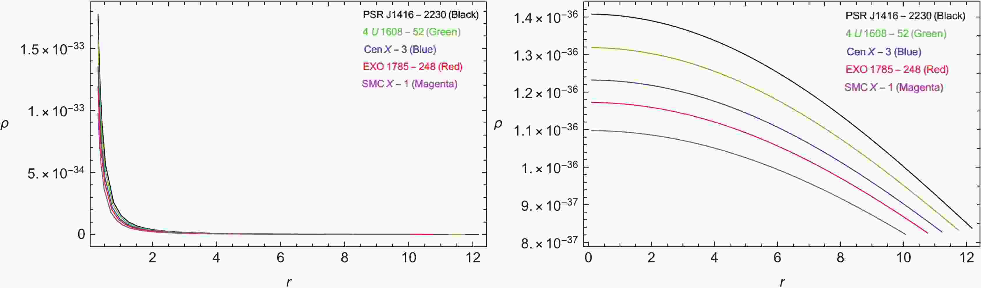
The physical admissibility of the stellar configurations in the compact star study is substantially important. If the study is not physically acceptable, it is worthless. Density is a useful parameter that ensures the admissibility of the case study. The justifiable nature of matter distribution is explained from the graphical behavior of the energy density ρ. Its following trend should be such that energy density must admit peak value in the center, and then decline toward the boundary, with a minimum value at the boundary (
$ r = R $ ). In addition, it must remain positive throughout the matter dispersal. Figure 1 illustrates the graphed behavior of ρ, which is maximum in the center at$ r = 0 $ . However, for$ n = 1 $ , it admits a sudden decline in its value, and for$ n = 2 $ it exhibits a regular decline and remains thoroughly positive in both cases, which is a crucial requirement. Therefore, energy density follows the admissible trend by ensuring the physical existence of the stellar bodies, which is a significant requirement in stellar studies, and for our case as well.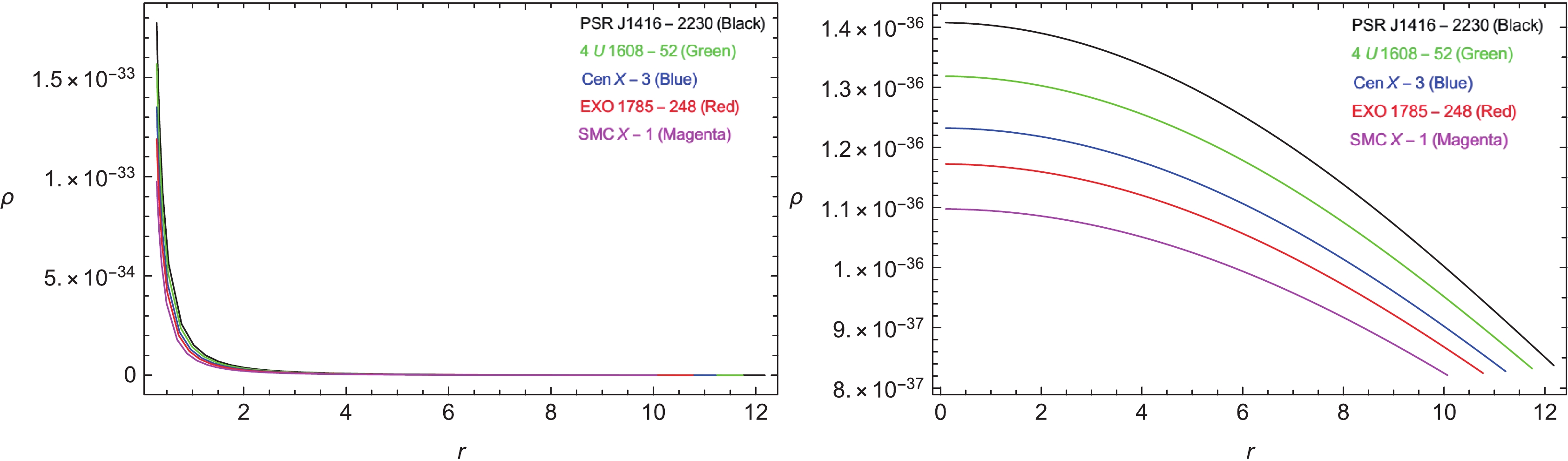
Figure 1. (color online) Density versus radial coordinate r for
$n=1$ (left) and$n=2$ (right). -
Pressure components are another necessary parameters in determining the admissibility of the stellar model. Considering the approaches that should be followed by the pressure components in the discussion of compact stars, parameter such as ρ,
$ p_r $ , and$ p_t $ must also remain positive throughout the stellar distribution by admitting peak values in the center, and then exhibiting a decline from the center to the boundary, with a minimum value at the boundary.$ p_t>p_r $ and$ p_r $ should vanish at the boundary ($ r = R $ ), and$ p_t $ should remain positive throughout the matter distribution. Figure 2 demonstrates that$ p_r $ and$ p_t $ have identical behaviors to ρ in both cases (for$ n = 1 $ both$ p_t $ and$ p_r $ have maximum values in the center, as well as a sudden decline from the peak value toward$ r = R $ , with a positive conduct; however, for$ n = 2 $ these parameters decline smoothly from the maximum to the minimum value), and remain in an admissible range, as$ p_r(r = R) = 0 $ , and$ p_t>p_r $ is positive at the boundary.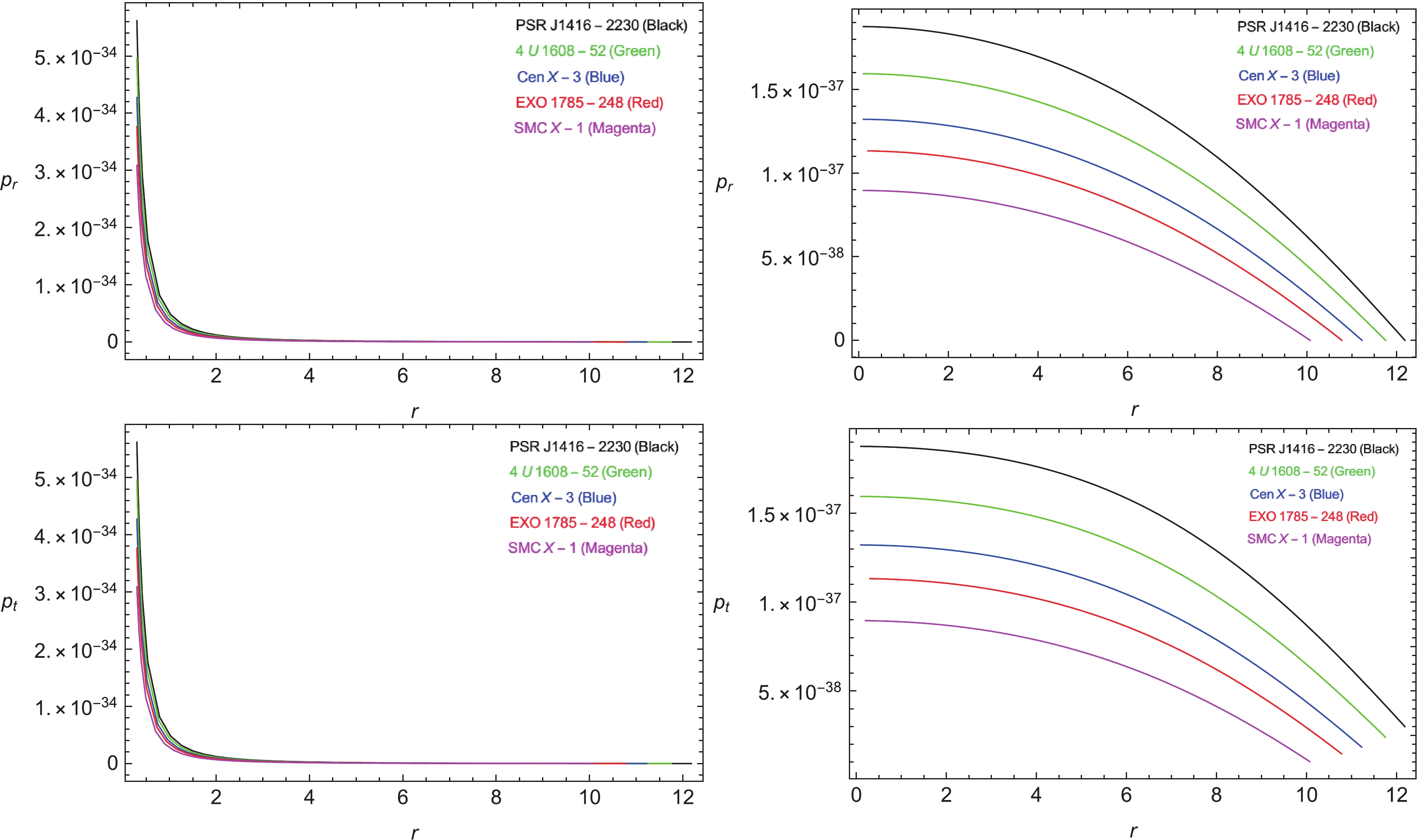
Figure 2. (color online) Radial and tangential pressures versus radial coordinate r for
$n=1$ (left) and$n=2$ (right). -
The admissible criteria for gradient components is that they should follow the negative trend in the anisotropic matter dispersal, i.e.
$ \frac{{\rm d}\rho}{{\rm d}r}\bigg|_{r = 0} = 0,\;\;\; \frac{{\rm d} p_t}{{\rm d}r}\bigg|_{r = 0} = 0,\;\;\; \frac{{\rm d} p_t}{{\rm d}r}\bigg|_{r = 0} = 0 $

(30) however, for other values of the radius r, i.e. from
$ 0<r\leqslant R $ , this trend should exist, such that:$ \frac{{\rm d}\rho}{{\rm d}r}\bigg|_{r = 0}<0,\;\;\; \frac{{\rm d} p_t}{{\rm d}r}\bigg|_{r = 0}<0,\;\;\; \frac{{\rm d} p_t}{{\rm d}r}\bigg|_{r = 0}<0. $

(31) Figure 3 illustrates the trend of gradients in our study. Accordingly, for
$ n = 1 $ , this trend progress from negative to zero, and for$ n = 2 $ , its progression is from zero to negative. However, in both cases, the gradients remain within the admissible range.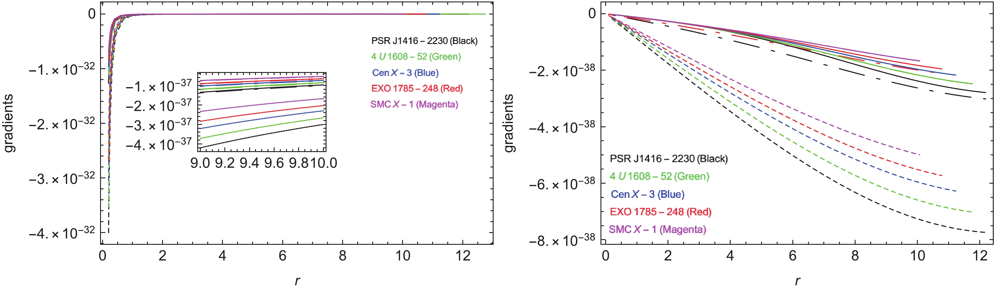
Figure 3. (color online) Gradients versus radial coordinate r for
$n=1$ (left) and$n=2$ (right). -
It is important to state that the positive anisotropy (
$ \Delta>0 $ , if$ p_t>p_r $ , as$ \Delta = p_t - p_r $ ) is an attestation for the exhibition of repulsive forces that counterbalance the gradients and improve the equilibrium and steadiness. Actually, this phenomenon allows more compact configurations [61] and huge massive formations. At the center where$ r = 0 $ , anisotropy is not present owing to the coincidence of pressures$ p_r $ and$ p_t $ . However, with the increase in radius, these quantities float separately; hence, anisotropy increases toward the boundary surface of the star. Figure 4 illustrates the positive and smooth behavior of$ \Delta $ for both values,$ n = 1 $ and$ n = 2 $ .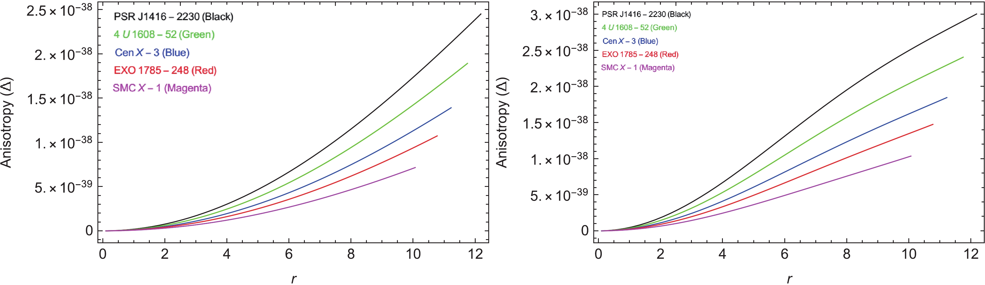
Figure 4. (color online) Anisotropy versus radial coordinate r for
$n=1$ (left) and$n=2$ (right). -
The EMT describes the mass, stress, and momentum in GR, which are considered for the existence of matter field and every other gravitation-free field (GFF). In the space-time model, the field equation did not directly concern the state of matter or allowable GFF. Conversely, energy conditions allow all forms of matter and diverse GFF in the GR theory and preserve the physically suitable solutions of filed equations. To realize the rational and physically reasonable distribution of anisotropic matter, field energy must remain positive throughout the stellar object; accordingly, some mathematical functions of inequalities must be satisfied. In the literature [62, 63], these energy conditions are discussed as null energy conditions (NEC), weak energy conditions (WEC), strong energy conditions (SEC), and dominant energy conditions (DEC), in terms of both the radial and tangential directions, given as:
$ \begin{array}{l} {\rm NEC}:\rho+p_\gamma\geqslant 0, \\ {\rm WEC}:\rho\geqslant 0,\;\;\;\rho+p_\gamma\geqslant 0, \\ {\rm SEC}:\rho+p_\gamma\geqslant 0,\;\;\;\rho+p_r+2p_t\geqslant 0, \\ {\rm DEC}:\rho>|p_\gamma|. \end{array}$

where (
$ \gamma = r, t $ ), and r and t are the notations used for radial and tangential coordinates, respecticely. Figure 5 is an indication towards the satisfaction of the above energy conditions in the framework of$ f(T, {\cal{T}}) $ gravity for our selected values of n, i.e.$ n = 1 $ and$ n = 2 $ .
Figure 5. (color online) Energy conditions versus radial coordinate r for
$n=1$ (left) and$n=2$ (right). -
In this section, we present the physical viability of the stellar solutions by discussing the matter nature, equilibrium, stability, and physical existence using EOS, TOV equations, casuality conditions, and mass function, respectively. In addition, we discuss compactness and redshift.
-
In the study of compact stars, it is important to discuss the importance of matter arrangements, whether it is normal or dark matter. For the normal arrangement of matter, both the tangential and radial components of EOS lie within the ranges
$ 0\leqslant w_r, \;w_t<1 $ . If the stellar object is composed of the realistic anisotropic matter, the results will satisfy this stability criteria. If the limits defined for EOS are violated, this might be an indication of exotic or dark matter. EOS is mathematically expreesed as:$ w_r = \frac{p_r}{\rho}, $

(32) $ w_t = \frac{p_t}{\rho}. $

(33) As observed in Fig. 6 , the graphical response of these EOS Eqs. (32) and (33) is presentd, which indicates that the distribution of matter is the normal one, as it satisfies the required range of stability in the effects of the
$ f(T,{\cal{T}}) $ gravity for our selected values,$ n = 1 $ for liner modification, and$ n = 2 $ for generic results.
Figure 6. (color online) EOS
$w_r$ (solid),$w_t$ (dotted) versus radial coordinate r for$n=1$ (left) and$n=2$ (right). -
The Tolman-Oppenheimer-Volkoff (TOV) equation [64, 65] is adopted as the equilibrium parameter. According to these TOV equations, the stellar system is in equilibrium state if it is well balanced under gravitational (
$ F_{\rm g} $ ), hydrostatic ($ F_{\rm h} $ ), anisotropic ($ F_{\rm a} $ ) fields. The TOV equation in its general form is given by:$ \frac{{\rm d} p_r}{{\rm d}r}+\frac{M_{\rm g} (r)(\rho+p_r)}{r}e^{\frac{\xi-\psi}{2}}- \frac{2(p_t-p_r)}{r} = 0, $

(34) where
$ M_{\rm g} (r) $ , which is the gravitational mass inside the radius r, and can be derived by the Tolman-Whittaker formula:$ M_{\rm g}(r) = 4\pi \int_{0}^{r}(T_{t}^{t}-T_{r}^{r}-T_{\theta}^{\theta}-T_{\phi}^{\phi})r^2e^{\frac{\xi+\psi}{2}}{\rm d}r. $

(35) The Eq. (34) can take the form given as:
$ M_{\rm g}(r) = \frac{2}{2}re^{\frac{\psi-\xi}{2}}\xi^{'}. $

(36) By substituting the value of
$ M_{\rm g}(r) $ from Eq. (35) into Eq. (33), we obtain:$ \frac{{\rm d} p_r}{{\rm d}r}+\frac{\xi^{'}(\rho+p_r)}{r}- \frac{2(p_t-p_r)}{r} = 0. $

(37) An extra force (
$ F_{\rm e} $ ) [52] in the effects of the$ f(T,{\cal{T}}) $ gravity is also present. These forces in mathematical formulation are obtained as:$ \begin{aligned}[b]\frac{{\rm d} p_r}{{\rm d}r}&+\frac{\xi^{'}(\rho+p_r)}{r}- \frac{2(p_t-p_r)}{r}\\ &-\frac{-\dfrac{1}{4} \alpha \dfrac{\partial {\rm{pr}}}{\partial r}-\alpha \dfrac{\partial {\rm{pt}}}{\partial r}+\dfrac{1}{4} \alpha \dfrac{\partial \rho }{\partial r}}{\dfrac{\alpha }{2}+4 \pi } = 0,\end{aligned} $

(38) $ F_{\rm g}+F_{\rm h}+F_{\rm a}+F_{\rm e} = 0, $

(39) where
$\begin{aligned}[b]& F_{\rm g} = -\frac{\xi^{'}(\rho+p_r)}{2}, \quad F_{\rm h} = -\frac{{\rm d} p_r}{{\rm d}r}, \quad F_{\rm a} = \frac{2(p_t-p_r)}{r}, \quad \\ &F_{\rm e} = -\frac{-\dfrac{1}{4} \alpha \dfrac{\partial {{p_r}}}{\partial r}-\alpha \dfrac{\partial {{p_t}}}{\partial r}+\dfrac{1}{4} \alpha \dfrac{\partial \rho }{\partial r}}{\dfrac{\alpha }{2}+4 \pi }. \end{aligned}$

(40) The actual equilibrium test of the stellar system involves the combined balanced effect of these forces.
$ F_{\rm h},\; F_{\rm e} $ and the repulsive anisotropic force$ F_{\rm a} $ inhibit the effect of the gravitational force$ F_{\rm g} $ . This mechanism prevents the stellar system from collapsing to a point singularity during the gravitational collapse. These forces can be investigated from Fig. 7. As can be observed from the figure, the negative and positive effects of these forces counter each other; hence, our system is in equilibrium for$ n = 1 $ and also for$ n = 2 $ , as demonstrated by the balancing effect of these forces.
Figure 7. (color online) Forces versus radial coordinate r for
$n=1$ (left) and$n=2$ (right). -
In this section, we elaborate the physically satisfactory model by describing the squares of radial and tangential sound speeds. In addition, with the justification of stability, another concern involving the distribution of anisotropic matter emerges, which is known as Herrera's cracking concept [66]. Under the cracking concept, the stability of the stellar solutions is studied based on the radial and transverse sound speeds (
$ v^{2}_{r} $ and$ v^{2}_{t} $ ). According to this concept, both sound speeds must satisfy the inequalities$ 0<v^{2}_{r},\;v^{2}_{t}<1 $ (i.e., both sound speeds must remain less than the speed of light c, and must be positive within the stellar body, with the speed of light$ c = 1 $ ). These sound speeds are written as:$ v^2_r = \frac{{\rm d} p_r}{{\rm d}\rho},\;\;\;\;\; v^2_t = \frac{{\rm d} p_t}{{\rm d}\rho}. $

(41) Later, Abreu et al. [67] presented another stability criteria. According to this criteria, the region is stable where
$ v^{2}_{r}>v^{2}_{t} $ , i.e. there is no change in$ v^{2}_{r}-v^{2}_{t} $ . Subsequently, this assumption was set as$ 0\leqslant\mid v^{2}_{t}-v^{2}_{r}\mid<1 $ . The presented behaviors in the upper and lower pannels of Fig. 8 show that the radial speed is perpetually greater than the tangential speed; hence, our solutions are adequately adjusted with the cracking. Figure 9 is also an admitted examination of Abreu concepts for both modifications i.e.,$ n = 1 $ and$ n = 2 $ , in the influential frame of the$ f(T,{\cal{T}}) $ gravity.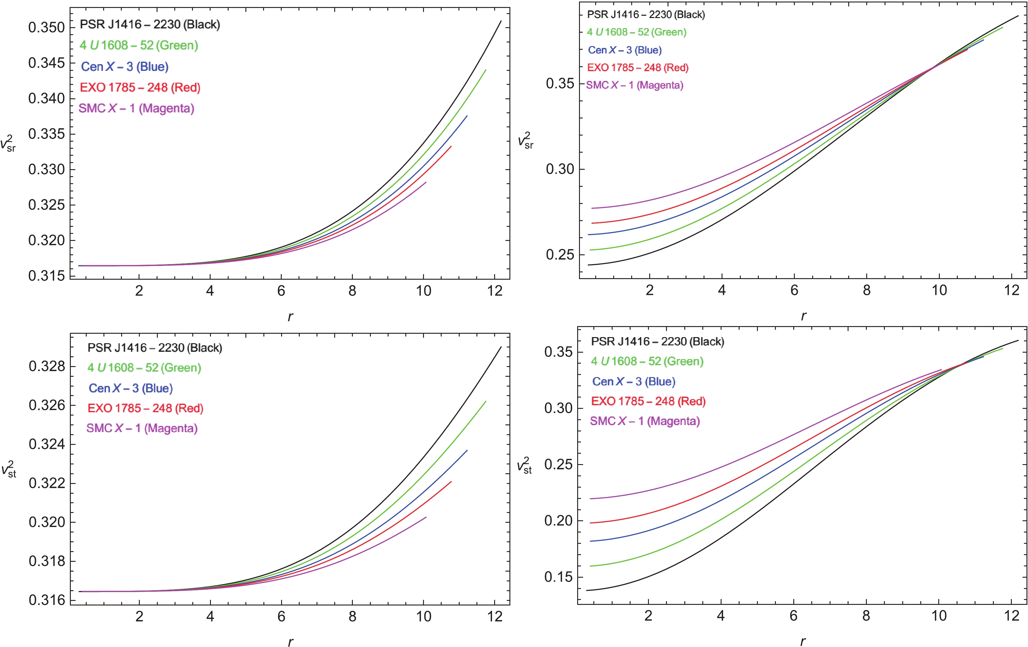
Figure 8. (color online) Velocities of sound versus radial coordinate r for
$n=1$ (left) and$n=2$ (right).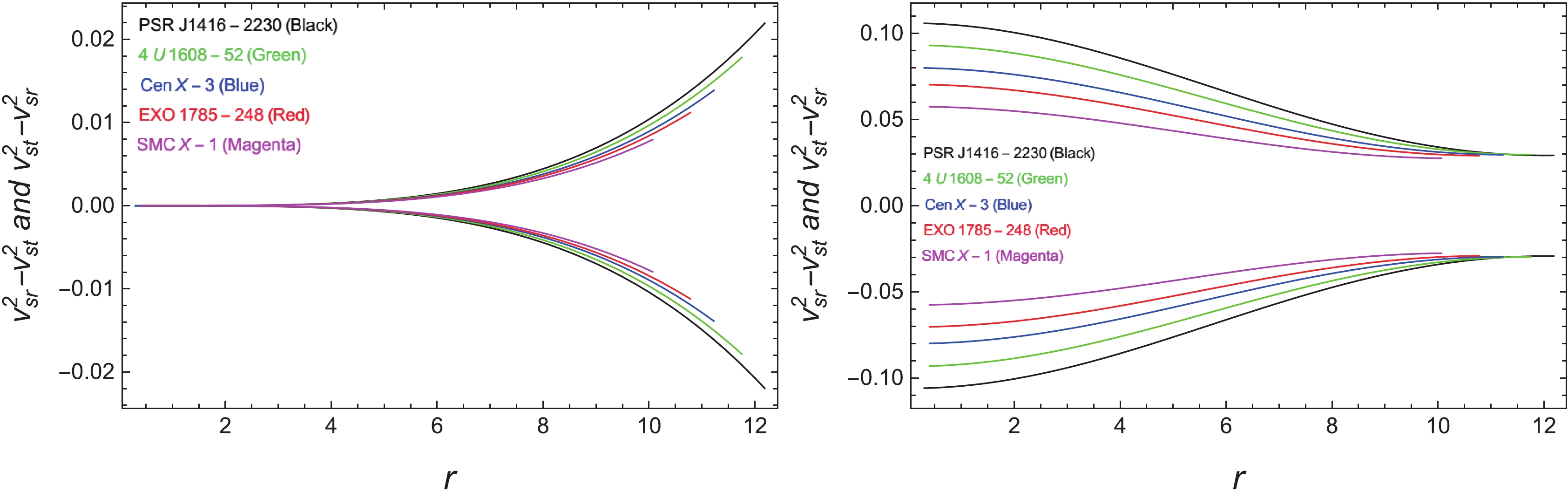
Figure 9. (color online) Stability factor versus radial coordinate r for
$n=1$ (left) and$n=2$ (right). -
The mass to radius ratio
$ \dfrac{m(r)}{R} $ is an important criteria for ascertaining the compactness level μ of the stellar object. The mass expression can be determined by using the mathematical form:$ m(R) = 4\pi\int r^2 \rho {\rm d}r. $

(42) Then, by adopting the above referenced Eq. (42), the relationship between compactness μ and redshift
$ z_s $ can be conveniently extracted as:$ u(r) = \frac{m(R)}{R}, $

(43) $ z_s = \left(1-2u\right)^{-\frac{1}{2}}-1. $

(44) In a simpler approach, the relationship for the mass function can be determined by using Eqs. (16) and (42), with the help of the metric component, as:
$ m(R) = \frac{R}{2}[1-e^{-\Psi[R]}]. $

(45) For the spherically symmetric distribution of matter contents, the maximum limit for compactification
$\mu = \dfrac{m}{r} < \dfrac{4}{9}$ [68] (in the unit system$ c = G = 1 $ ) must be satisfied. Subsequently, for the anisotropic matter, this limit was further generalized [69]. Figures 10-12 illustrate the realistic behavior of the mass function. The compactness factor is also within the Buchdhal limit, and the redshift function satisfies the criteria$ z_s\leqslant 4.77 $ [33]. By examining the graphs in Figs. 10-12, the realistic formation under the mass function, required compactification level, and stability of the system in both linear and non-linear modifications ($ n = 1 $ and$ n = 2 $ ) of the gravity theory can be concluded for compact star models.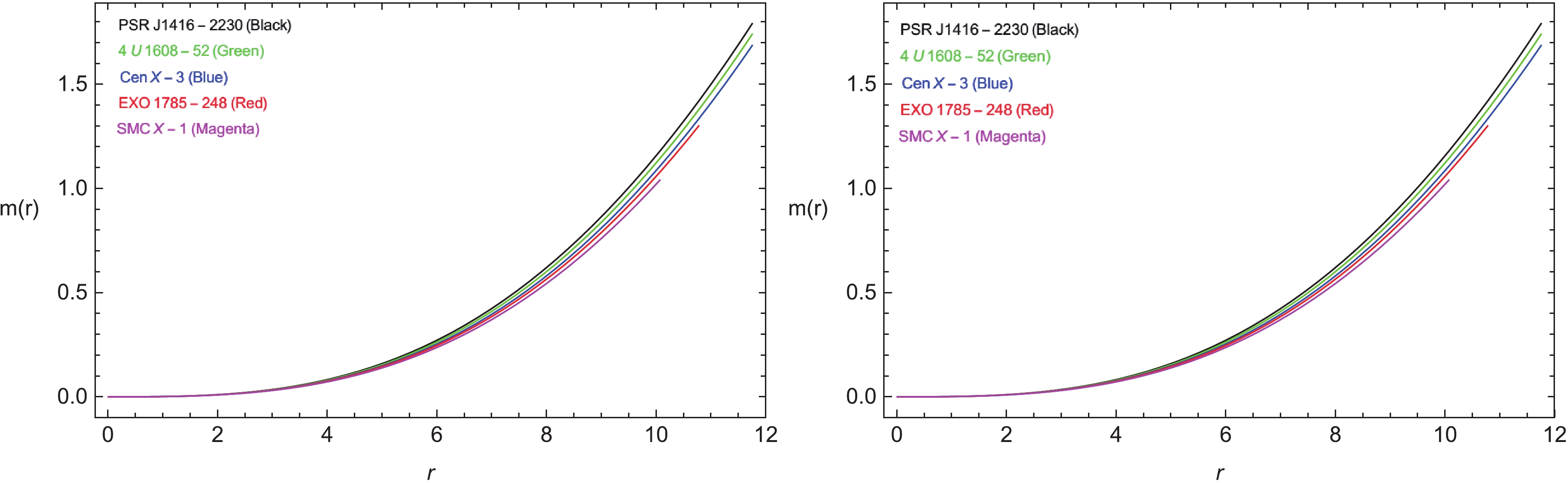
Figure 10. (color online) Mass function versus radial coordinate r for
$n=1$ (left) and$n=2$ (right).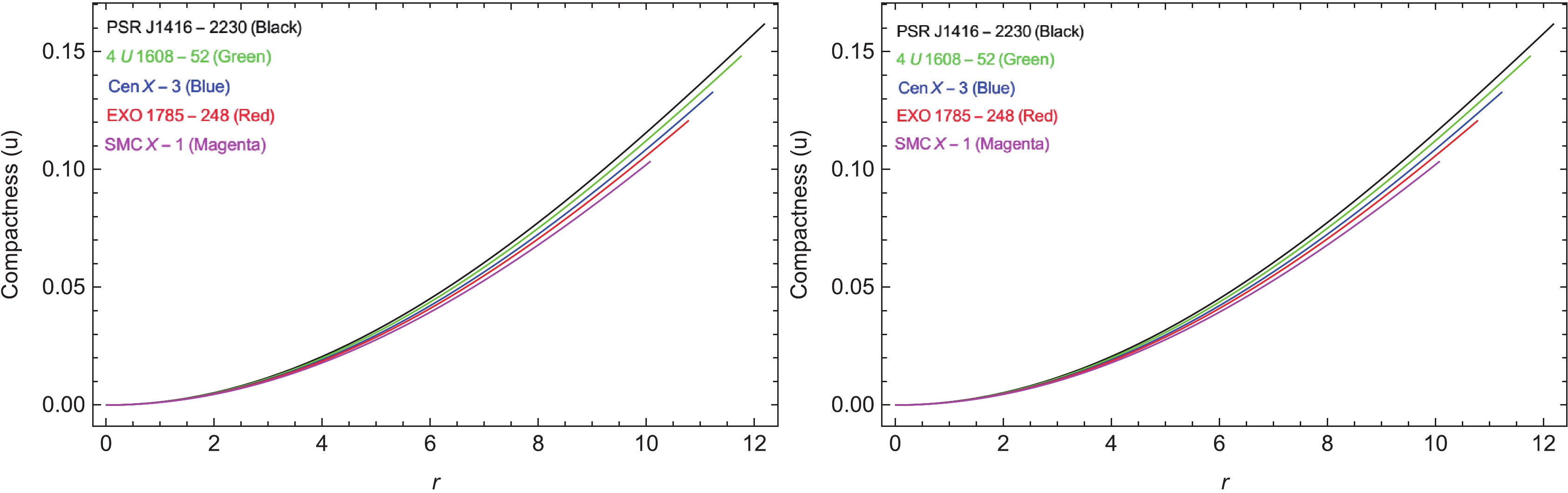
Figure 11. (color online) Compactness versus radial coordinate r for
$n=1$ (left) and$n=2$ (right).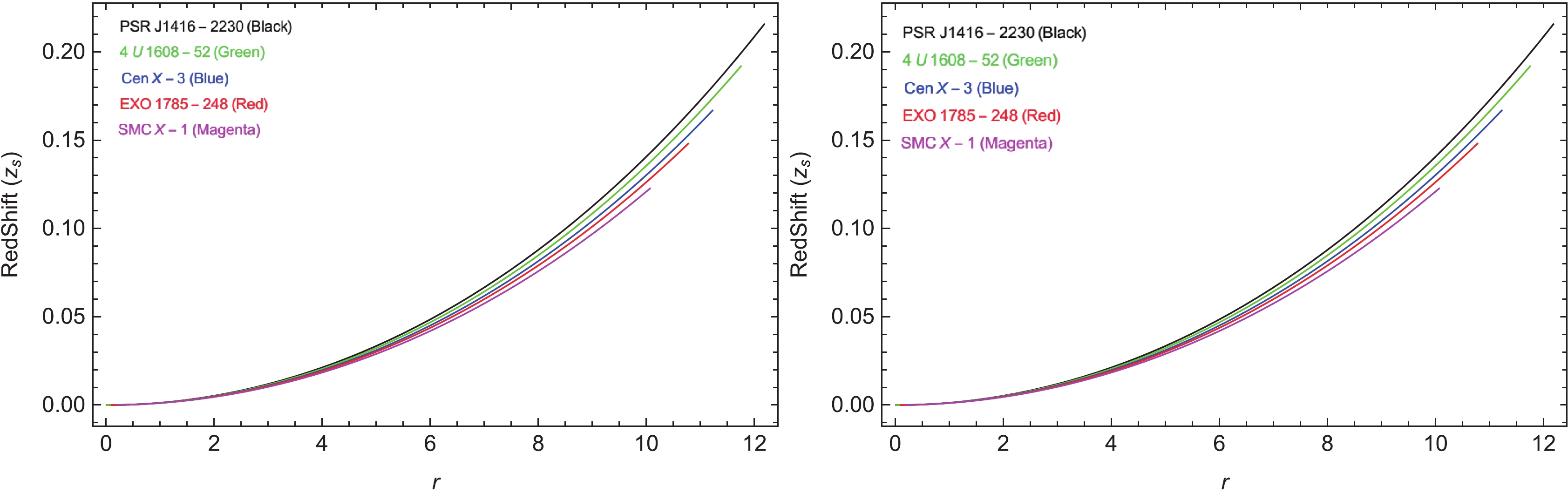
Figure 12. (color online) Redshift versus radial coordinate r for
$n=1$ (left) and$n=2$ (right). -
An essential parameter required to assume the stability factor of the relativistic and non-relativistic objects based on spherical symmetry is the adiabatic index. The adiabatic index analysis in the structure of spherical symmetric objects is a core component because it defines the stability and solidity of the EOS at the given density. Backing the pioneer work of Chandrasekhar [70, 71], several authors [72-75] presented the refined method for guessing the stability of the stellar objects that adopt the spherically symmetry, by adopting the adiabatic index. Based on the persepective of Heintzmann and Hillebrandt [76], the spherical symmetric stellar object is stable if its adiabatic index
$ \Gamma>\dfrac{4}{3} $ , throughout the interior of the stellar object. The dynamical adiabatic index is defined as:$ \Gamma = \frac{p_r + \rho}{p_r} v^{2}_r. $

(46) As the variation of adiabatic index versus radial coordinate can be examined from Fig. 13, it is evident that the condition
$ \Gamma>\dfrac{4}{3} $ is satisfid everwhere inside the stellar structure. Because$ \Gamma $ follows the complete conduct of Heintzmann and Hillebrandt [76], our stellar system is completely stable under the adiabatic index perturbation versus the radial coordinate for both values of n ($ n = 1,2 $ ).
Figure 13. (color online) Adiabatic index versus radial coordinate r for
$n=1$ (left) and$n=2$ (right). -
In this paper, we debated on the spherically symmetric solutions of compact stars by adopting the KB space time. In the literature [44-51], authors have developed stellar structures for compact star models using the KB space-time for spherical symmetry. Our main objective in this study was to elucidate the anisotropic effects of matter coupling in torsional gravity via the corrected and rotated tetrad formalisms. For this purpose, we adopted the KB model [47], as it is one of the simple models, and has never been used before in the
$ f(T, {\cal{T}}) $ gravity. First, we explored the comparative results of the linear$ n = 1 $ and non-linear$ n = 2 $ modification of$ f(T, {\cal{T}}) $ gravity by applying the model$ f(T,{\cal{T}}) = \alpha T^{n}(r)+ \beta {\cal{T}} (r)+ $ $ \phi $ a with a KB line-element. Accordingly, we employed the accessible data from available literature of five compact stars$ PSR J1416-2230 $ ,$ 4U 1608-52 $ ,$ Cen X-3 $ ,$ EXO 1785- $ $ 248 $ and$ SMC X-1 $ .To address the few solar system constraints that are present in the case of the diagonal tetrad, we adopt a non-diagonal in setting up$ f(T,{\cal{T}}) $ field equations. To accurately configure our solutions, we adopted$ f(T,{\cal{T}}) = \alpha T^{n}(r)+\beta {\cal{T}} (r)+\phi $ , an analytically and graphically suitable model of the$ f(T,{\cal{T}}) $ gravity. We applied the conventional matching condition for the evaluation of unknowns, whose values are presented in Table 1. We constructed our solutions for two values of n, i.e.$ n = 1,2 $ . Furthermore, we addressed the admissibility, stability, and physical existence of stellar objects by discussing the following stellar characteristics under the anisotropic effects of$ f(T,{\cal{T}}) $ gravity:● Energy density behaves optimally, as illustrated in Fig. 1. It meets the admissibility criteria, as it has its maximum value in the center, and starts to decrease toward the boundary. In addition, it remained positive throughout.
● Pressure components,
$ p_r $ and$ p_t $ , also exhibit an acceptable range under the realm of the$ f(T, {\cal{T}}) $ gravity, and both components follow the trend: In Fig. 2,$ p_r>0 $ and zero at the boundary,$ p_t>0 $ , and$ p_t>p_r $ . In addition, they exhibit their highest values in the center, and afterward exhibit a decline toward the boundary$ r = R $ .● Figure 3 clarifies that the gradients exhibit a negative trend via the stellar dispersal. As can be observed,
$\dfrac{{\rm d} \rho}{{\rm d}r}\leqslant 0$ ,$ \dfrac{{\rm d} p_r}{{\rm d}r}\leqslant 0 $ , and$ \dfrac{{\rm d} p_t}{{\rm d}r}\leqslant 0 $ . For$ n = 1 $ , gradients propagate from negative to zero, and for$ n = 2 $ , they propagate from zero to negative. However, both cases exhibit a negative behavior.● Figure 4 illustrates the expansion of anisotropy. As can be observed,
$ \Delta = 0 $ in the center ($ r = 0 $ ), where$ p_r = p_t $ . Subsequently, it shows a positive evolution ($ p_t>p_r $ ) by authenticating the occupancy of repulsive forces, which prevents the stellar objects from collapsing to a point singularity.● Positive trend of energy conditions indicate the ordinary nature of matter. Figure 5 demonstrates that in both cases considered in this study, energy remains positive, starting from the maximum value in the center to the minimum value at the boundary, with a sudden decline for
$ n = 1 $ and normal decline for$ n = 2 $ .● Tangential and radial components (
$ w_r,w_t $ ) investigate the matter composition of stellar objects to determine whether it is dark or ordinary matter. Figure 6 shows the normality of matter in both cases of this study ($ n = 1 $ and$ n = 2 $ ), as these components remain in the admitted range$ 0<w_r,w_t<1 $ .● Figure 7 presents the equilibrium of forces. The system is stable and in equilibrium if TOV forces are in balance, i.e. their combined effect is zero. In our study, all the forces
$ F_{\rm a} $ ,$ F_{\rm g} $ ,$ F_{\rm h} $ and$ F_{\rm e} $ are well balanced, and for$ n = 1 $ , the forces evolve from the negative and positive axes in the center and converge to zero at the boundary; however, for$ n = 2 $ , the forces propagate from zero (in center) to positive and negative axes (towards the boundary). By including these small positive and negative values, their net effect cancel each other.● As can be observed in Figs. 8 and 9, the causality (
$ 0<v_{r}^{2},v_{t}^{2}<1 $ ) and Abrue conditions ($ 0<\mid v_{r}^{2}-v_{t}^{2}\mid<1 $ ) (in both cases ($ n = 1,2 $ ) of our study) are optimally satisfied, and this indicates the stability of our solutions.● Figures 10-12 present the regularity mass function, as
$ r = 0 $ and,$ m = 0 $ , then it expands positively to the physical range of mass. The compactness factor also admits the Buchdahl criteria, whereas the redshift factor satisfies the limiting range$ z_s<4.77 $ .● Figure 13 also sufficiently validates the stability of our proposed stellar system under the behavioral response to the adiabatic index. It can be inferred that the adiabatic index in our study strictly followed the limit
$ \left(\Gamma>\dfrac{4}{3} \right)$ of stability.Moreover, it is important to note that in spite of being non-singular in nature, our solutions meet the Zeldovich stability condition
$ \dfrac{p_{rc}}{\rho}<1 $ at$ r\simeq0 $ . We have also tabulated these results in a summarized form to elucidate the discussed properties of compact stars, as presented in Table 2. Based on the above discussion on the properties of compact stars, we conclude that our compact star solutions, drawn from this manuscript, are physically admissible, graphically stable, and viable.Expression indicating the
property of compact starsRequired result $n=1$ 

$n=2$ 

Expression indicating the
property of compact starsRequired result $n=1$ 

$n=2$ 

ρ $>0$ 

Justified Justified $p_r$ 

$>0$ 

Justified Justified $p_t$ 

$>0$ 

Justified Justified $\dfrac{p_{rc}}{\rho_c}$ 

$\leqslant 1$ 

Justified Justified $\Delta$ 

$>0$ 

Justified Justified $\dfrac{{\rm d} \rho}{{\rm d}r}$ 

$<0$ 

Justified Justified $\dfrac{{\rm d} p_r}{{\rm d}r}$ 

$<0$ 

Justified Justified $\dfrac{{\rm d} p_t}{{\rm d}r}$ 

$<0$ 

Justified Justified $F_{\rm a}$ ,

$F_{\rm h}$ ,

$F_{\rm g}$ , and

$F_{\rm e}$ 

$Sum=0$ 

Justified Justified $\rho+p_r$ 

$>0$ 

Justified Justified $\rho+p_t$ 

$>0$ 

Justified Justified $\rho-p_r$ 

$>0$ 

Justified Justified $\rho-p_t$ 

$>0$ 

Justified Justified $\rho+p_r+2 p_t$ 

$>0$ 

Justified Justified $m(r)$ 

$>0$ 

Justified Justified $u(r)$ 

$0<u(r)<\dfrac{8}{9}$ 

Justified Justified $z_s$ 

$0<z_s)<5$ 

Justified Justified $w_r$ 

$0<w_r<1$ 

Justified Justified $w_t$ 

$0<w_r<1$ 

Justified Justified $v_{r}^{2}$ 

$0<v_{r}^{2}<1$ 

Justified Justified $v_{t}^{2}$ 

$0<v_{r}^{2}<1$ 

Justified Justified $v_{t}^{2}-v_{r}^{2}$ 

$-1<\mid v_{t}^{2}-v_{r}^{2}\mid<1$ 

Justified Justified Adiabatic index $\Gamma>\dfrac{4}{3}$ 

Justified Justified Table 2. Summary of calculated results using observed values of stars
${{PSR J1416-2230}}$ ,${{4U 1608-52}}$ ,${{Cen X-3}}$ ,${{EXO 1785-248}}$ , and${{SMC X-1}}$ . -
The authors thank the Higher Education Commission, Islamabad, Pakistan, for its financial support under the NRPU project, grant number: 7851/Balochistan/NRPU/R&D/HEC/2017.
Physical aspects of anisotropic compact stars in $ { {f(T,{\cal{T}})}}$ gravity with off diagonal tetrad
- Received Date: 2020-11-24
- Available Online: 2021-08-15
Abstract: This study addresses the formation of anisotropic compact star models in the background of


 DownLoad: