


 Abstract
 HTML
HTML Reference
 Related
 PDF
PDF


-
Today, nearly fifty years after the discovery of the
$ J/{\psi} $ particle in 1974 [1, 2], charmonium continues to be an interesting and exciting subject of research because it bridges the physics contents between the perturbative and nonperturbative energy scales and help elucidate the complex behavior and dynamics of strong interactions. In addition, the recent observations of exotic resonances beyond our comprehension, such as XYZs [3], have caused an upsurge of research on charmonium-like states and stimulated several experimental and theoretical activities.The
$ J/{\psi} $ particle, a system consisting of the charmed quark and antiquark pair$ c\bar{c} $ , is the lowest orthocharmonium state with the well established quantum number of$ J^{PC} $ $ = $ $ 1^{–} $ [3]. With the same quantum number$ J^{PC} $ as the photon, the$ J/{\psi} $ particle can be directly produced by$ e^{+}e^{-} $ annihilation. To date, there are more than$ 10^{10} $ $ J/{\psi} $ events available with the BESIII detector [4]. Considering the large$ J/{\psi} $ production cross section$ {\sigma} $ $ {\sim} $ $ 3400 $ $ {\rm nb} $ [5], it is expected that more than$ 10^{13} $ $ J/{\psi} $ events will be accumulated at the planning Super Tau Charm Facility (STCF) with$ 3\,{\rm ab}^{-1} $ on-resonance dataset in the future. The large amount of data provides a good opportunity for studying the properties of the$ J/{\psi} $ particle, understanding the strong interactions and hadronic dynamics, exploring novel phenomena, and searching for new physics (NP) beyond the standard model (SM).The mass of the
$ J/{\psi} $ particle,$ m_{\psi} $ $ = $ $ 3096.9 $ MeV [3], is below the open charm threshold. The$ J/{\psi} $ hadronic decays via the annihilation of$ c\bar{c} $ quark into gluons are of a higher order in the quark-gluon coupling$ {\alpha}_{s} $ and are therefore severely suppressed by the phenomenological Okubo-Zweig-Iizuka (OZI) rule [6-8]. The OZI suppression results in (1) the electromagnetic decay ratio having the same order of magnitude as its strong decay ratio,$ {\cal B}r(J/{\psi}{\to}{\gamma}^{\ast}{\to}{\ell}^{+}{\ell}^{-}+ \text{hadrons}) $ $ {\approx} $ 25% and$ {\cal B}r(J/{\psi}{\to}ggg) $ $ {\approx} $ 64% [3], and (2) a small decay width,$ {\Gamma}_{\psi} $ $ = $ $ 92.9{\pm}2.8 $ keV [3]. Generally, the more the number of particles in the final states, the more the effect of compact phase spaces resulting in a relatively less occurrence probability, and the lower the experimental signal reconstruction efficiency. The kinematics are simple for the$ J/{\psi} $ two-body decays. Given the conservation of quantum number$ J^{P} $ (i.e., the simultaneous conservation of both angular momentum and P parity) in the strong and electromagnetic interactions, the$ J/{\psi} $ $ {\to} $ $ PP $ ,$ PV $ ,$ VV $ ,$ SS $ ,$ SA $ ,$ AA $ decays originate from the P-wave contributions corresponding to the relative orbital angular momentum of the final states$ {\ell} $ $ = $ $ 1 $ and additional F-wave ($ {\ell} $ $ = $ $ 3 $ ) contributions to$ J/{\psi} $ $ {\to} $ $ VV $ ,$ AA $ decays, where P, V, S, and A represent the light$ SU(3) $ meson nonets, the pseudoscalar meson P with$ J^{P} $ $ = $ $ 0^{-} $ , vector meson V with$ J^{P} $ $ = $ $ 1^{-} $ , scalar meson S with$ J^{P} $ $ = $ $ 0^{+} $ , and axial-vector meson A with$ J^{P} $ $ = $ $ 1^{+} $ . The$ J/{\psi} $ $ {\to} $ $ PA $ ,$ VS $ ,$ VA $ decays emerge from the S-wave ($ {\ell} $ $ = $ $ 0 $ ) contributions, and additional D-wave ($ {\ell} $ $ = $ $ 2 $ ) contributions to$ J/{\psi} $ $ {\to} $ $ VS $ ,$ VA $ decays; however, the$ J/{\psi} $ $ {\to} $ $ PS $ decays are forbidden. Usually, the V, S and A mesons are unstable and decay immediately after their productions into many other particles. Experimentally, the branching ratios of the$ J/{\psi} $ $ {\to} $ $ PV $ decays for all the possible flavor-conservation combinations of final states, such as$ {\pi}{\rho} $ ,$ {\pi}{\omega} $ ,$ {\eta}^{(\prime)}{\rho} $ $ {\eta}^{(\prime)}{\omega} $ ,$ {\eta}^{(\prime)}{\phi} $ , and$ K\overline{K}^{\ast} $ , have been well determined, except for the double-OZI suppression$ {\pi}{\phi} $ mode [3]. For the$ J/{\psi} $ $ {\to} $ $ PP $ and$ VV $ decays, when the final states have explicit C-parity, the C invariance forbids these processes, and Bose symmetry strictly forbids two identical particles in the final states. Presently, only five branching ratios for the$ J/{\psi} $ $ {\to} $ $ {\pi}^{+}{\pi}^{-} $ ,$ K^{+}K^{-} $ ,$ K_{L}^{0}K_{S}^{0} $ ,$ K^{{\ast}{\pm}}\overline{K}^{{\ast}{\mp}} $ , and$ K^{{\ast}0}\overline{K}^{{\ast}0} $ decays have been quantitatively measured [3]. Theoretically, the$ J/{\psi} $ particle is widely regarded as a$ SU(3) $ singlet, and the possible admixture of light quarks is negligible. It is usually assumed [9-49] that the$ J/{\psi} $ decay into two mesons could be induced by the interferences of (a)$ c\bar{c} $ $ {\to} $ $ ggg $ $ {\to} $ $ q\bar{q} $ , where q denotes light quark, (b)$ c\bar{c} $ $ {\to} $ $ {\gamma}gg $ $ {\to} $ $ q\bar{q} $ , (c)$ c\bar{c} $ $ {\to} $ $ {\gamma}^{\ast} $ $ {\to} $ $ q\bar{q} $ , (d) the$ c\bar{c} $ $ {\leftrightarrow} $ $ q\bar{q} $ mixing, and (e) the virtual process$ c\bar{c} $ $ {\to} $ $ c\bar{q} $ $ + $ $ \bar{c}q $ $ {\to} $ $ q\bar{q} $ . Based on the quark model or unitary-symmetry schemes, the$ J/{\psi} $ $ {\to} $ $ PP $ ,$ PV $ decays via the strong and electromagnetic interactions have been extensively studied using phenomenological models, such as the vector meson dominance model in Refs. [9-20], and various parametrizations of the OZI$ J/{\psi} $ process in Refs. [21-45].Currently, the sum of all the measured branching ratio of exclusive
$ J/{\psi} $ decay modes, which include leptonic, hadronic, and radiative decay modes, is about 66% [3]; therefore, there are many other$ J/{\psi} $ decay modes yet to be experimentally determined and studied. In addition to the strong and electromagnetic decays, the$ J/{\psi} $ particle can also decay via the weak interactions within SM, although it is estimated that the branching ratios of$ J/{\psi} $ weak decays could be very small, approximately$ 2/{\tau}_{D}{\Gamma}_{\psi} $ $ {\sim} $ $ {\cal O}(10^{-8}) $ , where$ {\tau}_{D} $ and$ {\Gamma}_{\psi} $ are the lifetime of the charmed D meson and full width of the$ J/{\psi} $ particle, respectively. In principle, the$ J/{\psi} $ weak decays are possible in different ways: (a) the$ c\bar{c} $ pair annihilation into a virtual Z boson cascading into leptons or quarks, which is unsuitable for measurements owing to the serious pollution of strong and electromagnetic decays, (b) the W emission, (c) the W exchange, and (d) the flavor-changing-neutral currents. The characteristic signal of the W-emission$ J/{\psi} $ weak decays is a single charmed hadron in the final states. The semileptonic$ J/{\psi} $ $ {\to} $ $ D_{(s)}^{(\ast)} $ $ + $ $ {\ell}^{+}{\nu}_{\ell} $ decays and hadronic$ J/{\psi} $ $ {\to} $ $ D_{(s)}^{(\ast)} $ $ + $ X decays (where X$ = $ P, V) have been investigated experimentally [3, 50-53] and phenomenologically [54-67], where several different upper limits on branching ratios at a 90% confidence level are obtained mainly from BESII and BESIII experiments [50-53]. When the charmed hadrons are absent from the final states, the$ J/{\psi} $ weak decays into light hadrons could be induced by the W exchange interactions. It is generally thought that the amplitudes for the W-exchange decays are suppressed, relative to those for the W-emission decays. Only a few studies on W-exchange$ J/{\psi} $ weak decays exist [68-70]. The study of the$ J/{\psi} $ $ {\to} $ $ PP $ weak decays is helpful in testing the non-conservation of the C parity and strangeness quantum number. Based on the$ 1.3{\times}10^{9} $ $ J/{\psi} $ events collected with the BESIII detector, the upper limit on branching ratio for the C parity violating$ J/{\psi} $ $ {\to} $ $ K_{S}^{0}K_{S}^{0} $ decay,$ < $ $ 1.4{\times}10^{-8} $ , was recently obtained at a 95% confidence level [70]. Inspired by the potentials of BESIII and future STCP experiments, in this study, we examine the$ J/{\psi} $ decays into two pseudoscalar mesons via the W exchange interactions. Our study will provide a ready reference for future experimental investigations to further test SM and search for NP. -
The effective Hamiltonian governing the
$ J/{\psi} $ $ {\to} $ $ PP $ weak decay is expressed as [71],$ {\cal H}_{\rm eff}\ = \ \frac{G_{\rm F}}{\sqrt{2}}\, \sum\limits_{q_{1},q_{2}}\, V_{cq_{1}}\,V_{cq_{2}}^{\ast}\, \big\{ C_{1}({\mu})\,O_{1}({\mu}) +C_{2}({\mu})\,O_{2}({\mu}) \big\} +{\rm h.c.} , $

(1) where
$ G_{\rm F} $ $ {\simeq} $ $ 1.166{\times}10^{-5}\,{\rm GeV}^{-2} $ [3] is the Fermi coupling constant;$ V_{cq_{1,2}} $ is the Cabibbo-Kobayashi-Maskawa (CKM) element, and$ q_{1,2} $ $ {\in} $ {d, s}. The latest values of CKM elements from collected data are$ {\vert}V_{cd}{\vert} $ $ = $ $ 0.221{\pm}0.004 $ and$ {\vert}V_{cs}{\vert} $ $ = $ $ 0.987{\pm}0.011 $ [3]. The factorization scale$ {\mu} $ separates the physical contributions into short- and long-distance parts. The Wilson coefficients$ C_{1,2} $ summarize the short-distance physical contributions above the scales of$ {\mu} $ . They are computable with the perturbative field theory at the scale of the$ W^{\pm} $ boson mass$ m_{W} $ and then evolve into a characteristic scale of$ {\mu} $ for the c quark decay, based on the renormalization group equations.$ \vec{C}({\mu})\, = \, U_{4}({\mu},m_{b})\,M(m_{b})\,U_{5}(m_{b},m_{W})\, \vec{C}(m_{W}) , $

(2) where the explicit expression of the evolution matrix
$ U_{f}({\mu}_{f},{\mu}_{i}) $ and the threshold matching matrix$ M(m_{b}) $ can be found in Ref. [71]. The operators describing the local interactions among four quarks are defined as$ O_{1} = \big[ \bar{c}_{\alpha}\,{\gamma}_{\mu}\, (1-{\gamma}_{5})\,q_{1,{\alpha}} \big]\, \big[ \bar{q}_{2,{\beta}}\,{\gamma}^{\mu}\, (1-{\gamma}_{5})\,c_{\beta} \big] ,$

(3) $ O_{2} = \big[ \bar{c}_{\alpha}\,{\gamma}_{\mu}\, (1-{\gamma}_{5})\,q_{1,{\beta}} \big]\, \big[ \bar{q}_{2,{\beta}}\,{\gamma}^{\mu}\, (1-{\gamma}_{5})\,c_{\alpha} \big] , $

(4) where
$ {\alpha} $ and$ {\beta} $ are color indices.It should be noted that the contributions of penguin operators, being proportional to the CKM factors
$ V_{cd}\,V_{cd}^{\ast} $ $ + $ $ V_{cs}\,V_{cs}^{\ast} $ $ = $ $ -V_{cb}\,V_{cb}^{\ast} $ $ {\sim} $ $ {\cal O}({\lambda}^{4}) $ , are not considered here, because they are more suppressed than the tree contributions, where the CKM factors$ V_{cs}\,V_{cs}^{\ast} $ $ {\sim} $ $ {\cal O}(1) $ ,$ V_{cs}\,V_{cd}^{\ast} $ $ {\sim} $ $ {\cal O}({\lambda}) $ ,$ V_{cd}\,V_{cd}^{\ast} $ $ {\sim} $ $ {\cal O}({\lambda}^{2}) $ , and the Wolfenstein parameter$ {\lambda} $ $ {\approx} $ $ 0.2 $ .The decay amplitudes can be expressed as
$ {\cal A}(J/{\psi}{\to}PP)\, = \, \frac{G_{\rm F}}{\sqrt{2}}\, \sum\limits_{q_{1},q_{2}}\, V_{cq_{1}}\,V_{cq_{2}}^{\ast}\, \sum\limits_{i = 1}^{2}\, C_{i}({\mu})\,{\langle}PP{\vert} O_{i}({\mu})\, {\vert} J/{\psi} {\rangle} , $

(5) where the hadron transition matrix elements (HMEs)
$ {\langle}PP{\vert}O_{i}({\mu})\,{\vert}J/{\psi}{\rangle} $ $ = $ $ {\langle}O_{i}{\rangle} $ relate the quark operators with the concerned hadrons. Owing to the inadequate understanding of the hadronization mechanism, the remaining and most critical theoretical work is to properly compute HMEs. In addition, it is not difficult to imagine that the main uncertainties will come from HMEs containing nonperturbative contributions. -
In the past few years, several phenomenological models, such as the QCD factorization (QCDF) [72-77] and perturbative QCD (pQCD) approaches [78-84], have been fully developed and widely employed in evaluating HMEs. According to these phenomenological models, HMEs are usually expressed as the convolution of scattering amplitudes and the hadronic wave functions (WFs). The scattering amplitudes and WFs reflect the contributions at the quark and hadron levels, respectively. The scattering amplitudes describing the interactions between hard gluons and quarks are perturbatively calculable. WFs representing the momentum distribution of compositions in hadron are regarded as process independent and universal, and could be obtained by nonperturbative methods or from collected data. A potential disadvantage of the QCDF approach [72-77] in the practical calculation is that the annihilation contributions cannot be computed self-consistently, and other phenomenological parameters are introduced to deal with the soft endpoint divergences using the collinear approximation. With the pQCD approach [78-84], to regularize the endpoint contributions of the QCD radiative corrections to HMEs, the transverse momentum are suggested to be retained within the scattering amplitudes on one hand, and on the other hand, a Sudakov factor is introduced expressly for the WFs of all involved hadrons. Finally, the pQCD decay amplitudes are expressed as the convolution integral of three parts: the ultra-hard contributions embodied by Wilson coefficients
$ C_{i} $ , hard scattering amplitudes$ {\cal H} $ , and soft part contained in hadronic WFs$ {\Phi} $ .$ {\cal A}_{i} \, = \, \prod\limits_{j} {\int} {\rm d}x_{j}\,{\rm d}b_{j}\, C_{i}(t_{i})\,{\cal H}_{i}(t_{i},x_{j},b_{j})\, {\Phi}_{j}(x_{j},b_{j})\,{\rm e}^{-S_{j}} , $

(6) where
$ x_{j} $ represents the longitudinal momentum fraction of the valence quark,$ b_{j} $ is the conjugate variable of the transverse momentum, and$ {\rm e}^{-S_{j}} $ is the Sudakov factor. In this study, we adopt the pQCD approach to investigate the$ J/{\psi} $ $ {\to} $ $ PP $ weak decays within SM. -
For the
$ J/{\psi} $ $ {\to} $ $ PP $ weak decays, the valence quarks of the final states are entirely different from those of the initial state. Only annihilation configurations exist. Therefore, the$ J/{\psi} $ $ {\to} $ $ PP $ weak decays provide us with some typical processes to closely scrutinize the pure annihilation contributions. As an example, the Feynman diagrams for the$ J/{\psi} $ $ {\to} $ $ {\pi}^{-}K^{+} $ decay are shown in Fig. 1.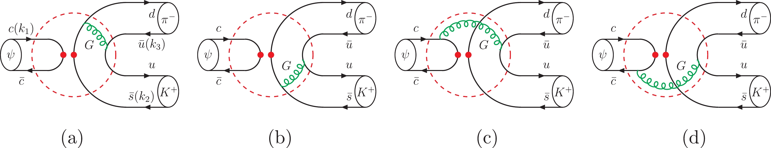
Figure 1. (color online) Feynman diagrams for the
$ J/{\psi} $ $ {\to} $ $ {\pi}^{-}K^{+} $ decay with the pQCD approach, where (a, b) are factorizable diagrams, and (c, d) are nonfactorizable diagrams. The dots denote appropriate interactions, and the dashed circles indicate scattering amplitudes.It is convenient to use the light-cone vectors to define the kinematic variables. In the rest frame of the
$ J/{\psi} $ particle, one has$ p_{\psi}\, = \, p_{1}\, = \, \frac{m_{\psi}}{\sqrt{2}}(1,1,0) , $

(7) $ p_{K}\, = \, p_{2}\, = \, \frac{m_{\psi}}{\sqrt{2}}(1,0,0) , $

(8) $ p_{\pi}\, = \, p_{3}\, = \, \frac{m_{\psi}}{\sqrt{2}}(0,1,0) , $

(9) $ k_{1}\, = \, x_{1}\,p_{1}+(0,0,\vec{k}_{1{\perp}}) , $

(10) $ k_{2}\, = \, x_{2}\,p_{2}^++(0,0,\vec{k}_{2{\perp}}) , $

(11) $ k_{3}\, = \, x_{3}\,p_{3}^-+(0,0,\vec{k}_{3{\perp}}) , $

(12) $ {\epsilon}_{\psi}^{\parallel}\, = \, \frac{1}{ \sqrt{2} }(1,-1,0) , $

(13) where
$ k_{i} $ ,$ x_{i} $ , and$ \vec{k}_{i{\perp}} $ represent the momentum, longitudinal momentum fraction, and transverse momentum, respectively. The quark momentum$ k_{i} $ is illustrated in Fig. 1(a).$ {\epsilon}_{\psi}^{\parallel} $ is the longitudinal polarization vector of the$ J/{\psi} $ particle and satisfies both the normalization condition$ {\epsilon}_{\psi}^{\parallel}{\cdot} {\epsilon}_{\psi}^{\parallel} $ $ = $ $ -1 $ and the orthogonal relation$ {\epsilon}_{\psi}^{\parallel}{\cdot}p_{\psi} $ $ = $ $ 0 $ . All hadrons are on mass shell, i.e.,$ p_{1} $ $ = $ $ m_{\psi}^{2} $ ,$ p_{2}^{2} $ $ = $ $ 0 $ and$ p_{3}^{2} $ $ = $ $ 0 $ . -
With the convention of Refs. [66, 85-87], the WFs and distribution amplitudes (DAs) are defined as
$ \begin{aligned}[b]& {\langle}\,0\,{\vert}\, \bar{c}_{\alpha}(0)\,c_{\beta}(z)\, {\vert} {\psi}(p_{1},{\epsilon}_{\parallel})\,{\rangle} \\ =& \, \frac{1}{4}\,f_{\psi}\, {\int}{\rm d}k_{1}\, {\rm e}^{+{\rm i}\,k_{1}{\cdot}z}\, \big\{ \!\not{\epsilon}_{\parallel} \big[ m_{\psi}\,{\phi}_{\psi}^{v} -\!\not{p}_{1}\, {\phi}_{\psi}^{t} \big] \big\}_{{\beta}{\alpha}} , \end{aligned} $

(14) $ \begin{aligned}[b]& {\langle}\,K(p_{2})\,{\vert}\, \bar{u}_{\alpha}(0)\, s_{\beta}(z)\, {\vert}\,0\,{\rangle} \\ = & -\frac{{\rm i}\,f_{K}}{4}\, {\int}{\rm d}k_{2}\, {\rm e}^{-{\rm i}\,k_{2}{\cdot}z}\, \Big\{ {\gamma}_{5}\, \big[ \!\not{p}_{2}\,{\phi}_{K}^{a} +{\mu}_{K}\,{\phi}_{K}^{p}\\& -{\mu}_{K}\, \big( \!\not{n}_+\!\not{n}_--1\Big)\, {\phi}_{K}^{t} \big] \big\}_{{\beta}{\alpha}} , \end{aligned} $

(15) $ \begin{aligned}[b]& {\langle}\,{\pi}(p_{3})\,{\vert}\, \bar{d}_{\alpha}(0)\, u_{\beta}(z)\, {\vert}\,0\,{\rangle} \\ = & -\frac{{\rm i}\,f_{\pi}}{4}\, {\int}{\rm d}k_{3}\, {\rm e}^{-{\rm i}\,k_{3}{\cdot}z}\, \big\{ {\gamma}_{5}\, \big[ \!\not{p}_{3}\,{\phi}_{\pi}^{a} +{\mu}_{\pi}\,{\phi}_{\pi}^{p}\\& -{\mu}_{\pi}\,\big( \!\not{n}_-\!\not{n}_+-1\big)\, {\phi}_{\pi}^{t} \big] \big\}_{{\beta}{\alpha}} , \end{aligned} $

(16) where
$ f_{\psi} $ ,$ f_{K} $ and$ f_{\pi} $ are decay constants;$ {\mu}_{K,{\pi}} $ $ = $ $ 1.6{\pm}0.2 $ GeV [86] is the chiral mass;$ n_{+} $ $ = $ $ (1,0,0) $ and$ n_{-} $ $ = $ $ (0,1,0) $ are the null vectors; and$ {\phi}_{P}^{a} $ and$ {\phi}_{P}^{p,t} $ are twist-2 and twist-3, respectively. The explicit expressions of$ {\phi}_{\psi}^{v,t} $ and$ {\phi}_{P}^{a,p,t} $ can be found in Ref. [66] and Refs. [86, 87], respectively. We collect these DAs as$ {\phi}_{\psi}^{v}(x) = A\, x\,\bar{x}\, {\exp}\Bigg( -\frac{m_{c}^{2}}{8\,{\omega}^{2}\,x\,\bar{x}} \Bigg) , $

(17) $ {\phi}_{\psi}^{t}(x) = B\, (\bar{x}-x)^{2}\, {\exp}\Bigg( -\frac{m_{c}^{2}}{8\,{\omega}^{2}\,x\,\bar{x}} \Bigg) , $

(18) $ {\phi}_{P}^{a}(x)\, = \, 6\,x\,\bar{x}\,\big\{ 1+a_{1}^{P}\,C_{1}^{3/2}({\xi}) +a_{2}^{P}\,C_{2}^{3/2}({\xi})\big\} , $

(19) $ \begin{aligned}[b] {\phi}_{P}^{p}(x) =& 1+3\,{\rho}_+^{P} -9\,{\rho}_-^{P}\,a_{1}^{P} +18\,{\rho}_+^{P}\,a_{2}^{P} \\ &+ \frac{3}{2}\,({\rho}_+^{P}+{\rho}_-^{P})\, (1-3\,a_{1}^{P}+6\,a_{2}^{P})\,{\ln}(x) \\& + \frac{3}{2}\,({\rho}_+^{P}-{\rho}_-^{P})\, (1+3\,a_{1}^{P}+6\,a_{2}^{P})\,{\ln}(\bar{x}) \\& - (\frac{3}{2}\,{\rho}_-^{P} -\frac{27}{2}\,{\rho}_+^{P}\,a_{1}^{P} +27\,{\rho}_-^{P}\,a_{2}^{P})\,C_{1}^{1/2}(\xi) \\& + ( 30\,{\eta}_{P}-3\,{\rho}_-^{P}\,a_{1}^{P} +15\,{\rho}_+^{P}\,a_{2}^{P})\,C_{2}^{1/2}(\xi) , \end{aligned} $

(20) $ \begin{aligned}[b] {\phi}_{P}^{t}(x) = & \frac{3}{2}\,({\rho}_-^{P}-3\,{\rho}_+^{P}\,a_{1}^{P} +6\,{\rho}_-^{P}\,a_{2}^{P}) \\& - C_{1}^{1/2}(\xi)\big\{ 1+3\,{\rho}_+^{P}-12\,{\rho}_-^{P}\,a_{1}^{P} +24\,{\rho}_+^{P}\,a_{2}^{P} \\ & + \frac{3}{2}\,({\rho}_+^{P}+{\rho}_-^{P})\, (1-3\,a_{1}^{P}+6\,a_{2}^{P})\,{\ln}(x) \\ & + \frac{3}{2}\,({\rho}_+^{P}-{\rho}_-^{P})\, (1+3\,a_{1}^{P}+6\,a_{2}^{P})\, {\ln}(\bar{x}) \big\} \\& - 3\,(3\,{\rho}_+^{P}\,a_{1}^{P} -\frac{15}{2}\,{\rho}_-^{P}\,a_{2}^{P})\,C_{2}^{1/2}(\xi) , \end{aligned} $

(21) where
$ \bar{x} $ $ = $ $ 1 $ $ - $ x and$ {\xi} $ $ = $ x$ - $ $ \bar{x} $ .$ {\omega} $ $ = $ $ m_{c}\,{\alpha}_{s}(m_{c}) $ is the shape parameter. The parameters A and B in Eqs. (17) and (18), respectively, are determined by the normalization conditions,$ {\int} {\phi}_{\psi}^{v,t}(x)\,{\rm d}x\, = \, 1 . $

(22) For the meaning and definition of other parameters, refer to Refs. [86, 87].
-
When the final states include the isoscalar
$ {\eta} $ or/and$ {\eta}^{\prime} $ , we assume that the glueball components, charmonium or bottomonium, are negligible. The physical$ {\eta} $ and$ {\eta}^{\prime} $ states are the mixtures of the$ SU(3) $ octet and singlet states, respectively. In our calculation, we will adopt the quark-flavor basis description proposed in Ref. [88], i.e.,$ \left( \begin{array}{c} {\eta} \\ {\eta}^{\prime} \end{array} \right)\, = \, \left(\begin{array}{cc} {\cos}{\phi} & -{\sin}{\phi} \\ {\sin}{\phi} & {\cos}{\phi} \end{array} \right)\, \left( \begin{array}{c} {\eta}_{q} \\ {\eta}_{s} \end{array} \right) , $

(23) where the mixing angle is
$ {\phi} $ $ = $ $ (39.3{\pm}1.0)^{\circ} $ [88];$ {\eta}_{q} $ $ = $ $ (u\bar{u}+d\bar{d})/{\sqrt{2}} $ and$ {\eta}_{s} $ $ = $ $ s\bar{s} $ . In addition, we assume that DAs of$ {\eta}_{q} $ and$ {\eta}_{s} $ are the same as those of pion; however, with different decay constants and mass [88-90],$ f_{q}\, = \, (1.07{\pm}0.02)\,f_{\pi} , $

(24) $ f_{s}\, = \, (1.34{\pm}0.06)\, f_{\pi} , $

(25) $ m_{{\eta}_{q}}^{2}\, = \, m_{\eta}^{2}\,{\cos}^{2}{\phi} +m_{{\eta}^{\prime}}^{2}\,{\sin}^{2}{\phi} -\frac{\sqrt{2}\,f_{s}}{f_{q}} (m_{{\eta}^{\prime}}^{2}- m_{\eta}^{2})\, {\cos}{\phi}\,{\sin}{\phi} , $

(26) $ m_{{\eta}_{s}}^{2}\, = \, m_{\eta}^{2}\,{\sin}^{2}{\phi} +m_{{\eta}^{\prime}}^{2}\,{\cos}^{2}{\phi} -\frac{f_{q}}{\sqrt{2}\,f_{s}} (m_{{\eta}^{\prime}}^{2}- m_{\eta}^{2})\, {\cos}{\phi}\, {\sin}{\phi} . $

(27) For the C parity violating
$ J/{\psi} $ decays, the amplitudes are$ \begin{aligned}[b] {\cal A}(J/{\psi}{\to}{\pi}^{0}{\eta}_{q}) =& -\frac{G_{\rm F}}{2\,\sqrt{2}}\, V_{cd}\,V_{cd}^{\ast}\, \big\{ a_{2}\, \big[ {\cal A}_{ab}({\pi},{\eta}_{q}) \\ &+ {\cal A}_{ab}({\eta}_{q},{\pi}) \big] + C_{1}\, \big[ {\cal A}_{cd}({\pi},{\eta}_{q}) \\ &+ {\cal A}_{cd}({\eta}_{q},{\pi}) \big] \big\} , \end{aligned} $

(28) $ {\cal A}(J/{\psi}{\to}{\pi}^{0}{\eta}) \, = \, {\cal A}(J/{\psi}{\to}{\pi}^{0}{\eta}_{q})\,{\cos}{\phi} , $

(29) $ {\cal A}(J/{\psi}{\to}{\pi}^{0}{\eta}^{\prime}) \, = \, {\cal A}(J/{\psi}{\to}{\pi}^{0}{\eta}_{q})\,{\sin}{\phi} , $

(30) $ \begin{aligned}[b] {\cal A}(J/{\psi}{\to}{\eta}_{s}{\eta}_{s}) = & \sqrt{2}\,G_{\rm F}\, V_{cs}\,V_{cs}^{\ast}\, \big\{ a_{2}\,{\cal A}_{ab}({\eta}_{s},{\eta}_{s}) \\ &+C_{1}\,{\cal A}_{cd}({\eta}_{s},{\eta}_{s}) \big\} , \end{aligned} $

(31) $ \begin{aligned}[b] {\cal A}(J/{\psi}{\to}{\eta}_{q}{\eta}_{q})= & \frac{G_{\rm F}}{\sqrt{2}}\, V_{cd}\,V_{cd}^{\ast}\, \big\{ a_{2}\,{\cal A}_{ab}({\eta}_{q},{\eta}_{q}) \\ &+C_{1}\,{\cal A}_{cd}({\eta}_{q},{\eta}_{q}) \big\} , \end{aligned} $

(32) $ \begin{aligned}[b] {\cal A}(J/{\psi}{\to}{\eta}{\eta}^{\prime}) = & \big\{ {\cal A}(J/{\psi}{\to}{\eta}_{q}{\eta}_{q})\\ &-{\cal A}(J/{\psi}{\to}{\eta}_{s}{\eta}_{s}) \big\}\, {\sin}{\phi}\,{\cos}{\phi} . \end{aligned}$

(33) For the strangeness changing
$ J/{\psi} $ decays, the amplitudes are$ \begin{aligned}[b] {\cal A}(J/{\psi}{\to}{\pi}^-K^+) = & \frac{G_{\rm F}}{\sqrt{2}}\, V_{cs}\,V_{cd}^{\ast}\, \big\{ a_{2}\,{\cal A}_{ab}({\pi},K) \\ &+C_{1}\,{\cal A}_{cd}({\pi},K) \big\} , \end{aligned}$

(34) $ \begin{aligned}[b] {\cal A}(J/{\psi}{\to}{\pi}^{0}K^{0}) = & -\frac{G_{\rm F}}{2}\, V_{cs}\,V_{cd}^{\ast}\, \big\{ a_{2}\,{\cal A}_{ab}({\pi},K) \\ &+C_{1}\,{\cal A}_{cd}({\pi},K) \big\} , \end{aligned} $

(35) $ \begin{aligned}[b]{\cal A}(J/{\psi}{\to}K^{0}{\eta}_{s}) =& \frac{G_{\rm F}}{\sqrt{2}}\, V_{cs}\,V_{cd}^{\ast}\, \big\{ a_{2}\,{\cal A}_{ab}(K,{\eta}_{s}) \\ &+C_{1}\, {\cal A}_{cd}(K,{\eta}_{s}) \big\} , \end{aligned}$

(36) $ \begin{aligned}[b] {\cal A}(J/{\psi}{\to}K^{0}{\eta}_{q}) =& \frac{G_{\rm F}}{2}\, V_{cs}\,V_{cd}^{\ast}\, \big\{ a_{2}\,{\cal A}_{ab}({\eta}_{q},K) \\ &+C_{1}\, {\cal A}_{cd}({\eta}_{q},K) \big\} , \end{aligned}$

(37) $ \begin{aligned}[b]{\cal A}(J/{\psi}{\to}K^{0}{\eta}) = & {\cal A}(J/{\psi}{\to}K^{0}{\eta}_{q})\, {\cos}{\phi} \\ &-{\cal A}(J/{\psi}{\to}K^{0}{\eta}_{s})\, {\sin}{\phi} ,\end{aligned} $

(38) $\begin{aligned}[b] {\cal A}(J/{\psi}{\to}K^{0}{\eta}^{\prime}) = & {\cal A}(J/{\psi}{\to}K^{0}{\eta}_{q})\, {\sin}{\phi} \\ &+{\cal A}(J/{\psi}{\to}K^{0}{\eta}_{s})\, {\cos}{\phi} , \end{aligned} $

(39) where coefficient
$ a_{2} $ $ = $ $ C_{1} $ $ + $ $ C_{2}/N_{c} $ and the color number$ N_{c} $ $ = $ $ 3 $ . The amplitude building blocks$ {\cal A}_{ij} $ are listed in Appendix A. From the above amplitudes, it is foreseeable that if the$ J/{\psi} $ $ {\to} $ $ {\pi}{\eta}^{({\prime})} $ decays are experimentally observed, the CKM element$ |V_{cd}| $ can be constrained or extracted. -
The branching ratio is defined as
$ {\cal B}r \, = \, \frac{p_{\rm cm}}{24\,{\pi}\,m_{\psi}^{2}\,{\Gamma}_{\psi}}\, {\vert} {\cal A}(J/{\psi}{\to}PP) {\vert}^{2} , $

(40) where
$ p_{\rm cm} $ is the center-of-mass momentum of final states in the rest frame of the$ J/{\psi} $ particle. Using the inputs in Table 1, the numerical results of branching ratios are obtained and presented in Table 2. Our comments on the results are presented as follows:mass, width, and decay constants of the particles [3] $ m_{{\pi}^{0}} $ 

$ = $ 

$ 134.98 $ MeV,

$ m_{K^{0}} $ 

$ = $ 

$ 497.61 $ MeV,

$ f_{{\pi}} $ 

$ = $ 

$ 130.2{\pm}1.2 $ MeV,

$ m_{{\pi}^{\pm}} $ 

$ = $ 

$ 139.57 $ MeV,

$ m_{K^{\pm}} $ 

$ = $ 

$ 493.68 $ MeV,

$ f_{K} $ 

$ = $ 

$ 155.7{\pm}0.3 $ MeV,

$ m_{\eta} $ 

$ = $ 

$ 547.86 $ MeV,

$ m_{{\eta}^{\prime}} $ 

$ = $ 

$ 957.78 $ MeV,

$ f_{\psi} $ 

$ = $ 

$ 395.1{\pm}5.0 $ MeV [66],

$ m_{c} $ 

$ = $ 

$ 1.67{\pm}0.07 $ GeV,

$ m_{J/{\psi}} $ 

$ = $ 

$ 3096.9 $ MeV,

$ {\Gamma}_{\psi} $ 

$ = $ 

$ 92.9{\pm}2.8 $ keV,

Gegenbauer moments at the scale of $ {\mu} $ 

$ = $ 1 GeV [86]

$ a_{1}^{\pi} $ 

$ = $ 

$ 0 $ ,

$\qquad a_{2}^{\pi} $ 

$ = $ 

$ 0.25{\pm}0.15 $ ,

$\qquad a_{1}^{K} $ 

$ = $ 

$ 0.06{\pm}0.03 $ ,

$\qquad a_{2}^{K} $ 

$ = $ 

$ 0.25{\pm}0.15 $ 

Table 1. Values of the input parameters, with their central values regarded as the default inputs, unless otherwise specified.
C parity violating decay modes mode $ {\cal B}r $ 

mode $ {\cal B}r $ 

$ J/{\psi} $ 

$ {\to} $ 

$ {\pi}^{0}{\eta} $ 

$ ( 2.32^{+ 0.81}_{- 0.24}){\times}10^{-14} $ 

$ J/{\psi} $ 

$ {\to} $ 

$ {\eta}{\eta}^{\prime} $ 

$ ( 3.01^{+ 0.78}_{- 0.55}){\times}10^{-11} $ 

$ J/{\psi} $ 

$ {\to} $ 

$ {\pi}^{0}{\eta}^{\prime} $ 

$ ( 1.45^{+ 0.50}_{- 0.15}){\times}10^{-14} $ 

the strangeness changing decay modes mode $ {\cal B}r $ 

mode $ {\cal B}r $ 

$ J/{\psi} $ 

$ {\to} $ 

$ {\pi}^{-}K^{+} $ 

$ ( 0.99^{+ 0.33}_{- 0.15}){\times}10^{-12} $ 

$ J/{\psi} $ 

$ {\to} $ 

$ K^{0}{\eta} $ 

$ ( 0.84^{+ 0.25}_{- 0.22}){\times}10^{-13} $ 

$ J/{\psi} $ 

$ {\to} $ 

$ {\pi}^{0}K^{0} $ 

$ ( 0.49^{+ 0.16}_{- 0.08}){\times}10^{-12} $ 

$ J/{\psi} $ 

$ {\to} $ 

$ K^{0}{\eta}^{\prime} $ 

$ ( 1.94^{+ 0.30}_{- 0.25}){\times}10^{-12} $ 

Table 2. Branching ratios for the
$ J/{\psi} $ $ {\to} $ $ PP $ weak decays, where the uncertainties originate from mesonic DAs, including the parameters of$ m_{c} $ ,$ {\mu}_{P} $ , and$ a_{2}^{P} $ .(1) The
$ J/{\psi} $ $ {\to} $ $ {\eta}{\eta}^{\prime} $ decays are Cabibbo-favored. The$ J/{\psi} $ $ {\to} $ $ K{\pi} $ and$ K{\eta}^{({\prime})} $ decays are singly Cabibbo-suppressed. The$ J/{\psi} $ $ {\to} $ $ {\pi}{\eta}^{({\prime})} $ decays are doubly Cabibbo-suppressed. Therefore, there is a hierarchical structure, i.e.,$ {\cal B}r(J/{\psi}{\to} {\eta}{\eta}^{\prime}) $ $ {\sim} $ $ {\cal O}(10^{-11}) $ ,$ {\cal B}r(J/{\psi}{\to}K{\pi},K{\eta}^{({\prime})}) $ $ {\sim} $ $ {\cal O}(10^{-12}- $ $ 10^{-13}) $ and$ {\cal B}r(J/{\psi}{\to} {\pi}{\eta}^{({\prime})} ) $ $ {\sim} $ $ {\cal O}(10^{-14}) $ .(2) Compared with the external W-emission induced
$ J/{\psi} $ $ {\to} $ $ D_{(s)}M $ decays, the internal W-exchange induced$ J/{\psi} $ $ {\to} $ $ PP $ decays are color-suppressed because the two light valence quarks of the effective operators belong to different final states. In addition, according to the the power counting rule of the QCDF approach in the heavy quark limit, the annihilation amplitudes are assumed to be power suppressed, relative to the emission amplitudes [73]. Therefore, the branching ratios for$ J/{\psi} $ $ {\to} $ $ PP $ decays are less than those for the$ J/{\psi} $ $ {\to} $ $ D_{(s)}M $ decays by one or two orders of magnitude [63-67].(3) The nonperturbative mesonic DAs are the essential parameters of the amplitudes with the pQCD approach. One of the main theoretical uncertainties emerging from participating DAs is given in Table 2. In addition, there are several other influence factors. For example, the decay constant
$ f_{\psi} $ and width$ {\Gamma}_{\psi} $ will bring 2.5% and 3% uncertainties to branching ratios.(4) Branching ratios for the
$ J/{\psi} $ $ {\to} $ $ {\eta}{\eta}^{\prime} $ decays can reach up to the order of$ 10^{-11} $ , which are far beyond the measurement precision and capability of current BESIII experiment; however, they might be accessible at the future high-luminosity STCF experiment. It will be very difficult and challenging but interesting to search for the$ J/{\psi} $ $ {\to} $ $ PP $ weak decays experimentally. It could be speculated that branching ratios for the$ J/{\psi} $ $ {\to} $ $ PP $ weak decays might be enhanced by including some novel interactions of NP models. For example, it has been shown in Refs. [91, 92] that the branching ratios for the W-emission$ J/{\psi} $ $ {\to} $ D$ + $ X weak decays could be as large as$ 10^{-6} $ $ {\sim} $ $ 10^{-5} $ , with the contributions from NP. An observation of the phenomenon of an abnormally large occurrence probability would be a hint of NP. -
Within the SM, the C parity violating
$ J/{\psi} $ $ {\to} $ $ {\pi}^{0}{\eta}^{(\prime)} $ and$ {\eta}{\eta}^{\prime} $ decays and the strangeness changing$ J/{\psi} $ $ {\to} $ $ K{\pi} $ and$ K{\eta}^{(\prime)} $ decays are solely valid and possible via the weak interactions; however, they are very rare. In this study, based on the latest progress and future prospects of the$ J/{\psi} $ physics at high-luminosity collider, we studied the$ J/{\psi} $ $ {\to} $ $ PP $ weak decays using the pQCD approach for the first time. It is determined that the branching ratios for the$ J/{\psi} $ $ {\to} $ $ {\eta}{\eta}^{\prime} $ decays can reach up to the order of$ 10^{-11} $ , which might be measurable by the future STCF experiment. -
From the definitions of Eqs. (15) and (16), it can be clearly observed that the twist-3 DAs are always accompanied by a chiral mass
$ {\mu}_{P} $ . Using the pQCD approach, a Sudakov factor is introduced for each of the hadronic WFs.We take the
$ J/{\psi} $ $ {\to} $ $ K^{+}{\pi}^{-} $ decay as an example. For simplicity, we use the following shorthand forms:$ {\phi}_{\psi}^{v,t} \, = \, {\phi}_{\psi}^{v,t}(x_{1})\,{\rm e}^{-S_{\psi}} , \tag{A1}$

$ {\phi}_{K}^{a} \, = \, {\phi}_{K}^{a}(x_{2})\,{\rm e}^{-S_{K}} , \tag{A2} $

$ {\phi}_{K}^{p,t} \, = \, \frac{ {\mu}_{K} }{ m_{\psi} }\, {\phi}_{K}^{p,t}(x_{2})\,{\rm e}^{-S_{K}} , \tag{A3} $

$ {\phi}_{\pi}^{a} \, = \, {\phi}_{\pi}^{a}(x_{3})\,{\rm e}^{-S_{\pi}} , \tag{A4} $

$ {\phi}_{\pi}^{p,t} \, = \, \frac{ {\mu}_{\pi} }{ m_{\psi} }\, {\phi}_{\pi}^{p,t}(x_{3})\,{\rm e}^{-S_{\pi}} , \tag{A5} $

where the definitions of Sudakov factors are
$ S_{\psi} = s(x_{1},p_{1}^+,b_{1}) +2\,{\int}_{1/b_{1}}^{t} \frac{{\rm d}{\mu}}{{\mu}}{\gamma}_{q} , \tag{A6}$

$ S_{K} = s(x_{2},p_{2}^+,b_{2}) +s(\bar{x}_{2},p_{2}^+,1/b_{2}) +2{\int}_{1/b_{2}}^{t} \frac{{\rm d}{\mu}}{{\mu}}{\gamma}_{q} , \tag{A7} $

$ S_{\pi} \!=\! s(x_{3},p_{3}^-,b_{3}) \!+\!s(\bar{x}_{3},p_{3}^-,1/b_{3}) \!+\!2{\int}_{1/b_{3}}^{t} \frac{{\rm d}{\mu}}{{\mu}}{\gamma}_{q} .\!\!\! \tag{A8} $

The
$ s(x,Q,b) $ expression can be found in Ref. [80].$ {\gamma}_{q} = $ $ -{\alpha}_{s}/{\pi} $ is the quark anomalous dimension. In addition, the decay amplitudes are always the functions of Wilson coefficient$ C_{i} $ . It should be understood that the shorthand$ C_{i}\, {\cal A}_{jk}({\pi},K) \, = \, \frac{{\pi}\,C_{\rm F}}{N_{c}}\, m_{\psi}^{4}\,f_{\psi}\,f_{K}\,f_{\pi}\, \big\{ {\cal A}_{j}(C_{i}) + {\cal A}_{k}(C_{i}) \big\} , \tag{A9} $

where the color factor
$ C_{F} $ $ = $ $ 4/3 $ and the color number$ N_{c} $ $ = $ $ 3 $ . The subscripts j and k of building block$ {\cal A}_{j(k)} $ correspond to the indices of Fig. 1. The expressions of$ {\cal A}_{i} $ are written as$ {\cal A}_{a} = {\int}_{0}^{1}{\rm d}x_{2}\,{\rm d}x_{3} {\int}_{0}^{\infty}{\rm d}b_{2}\,{\rm d}b_{3}\, H_{ab}({\alpha}_{g},{\beta}_{a},b_{2},b_{3})\, {\alpha}_{s}(t_{a})\,C_{i}(t_{a}) S_{t}(\bar{x}_{2})\, \big\{ {\phi}_{K}^{a}\,{\phi}_{\pi}^{a}\,\bar{x}_{2} -2\,{\phi}_{\pi}^{p}\, \big[ {\phi}_{K}^{p}\,x_{2} + {\phi}_{K}^{t}\,( 1+\bar{x}_{2} ) \big] \big\} , \tag{A10}$ 
$ {\cal A}_{b} = {\int}_{0}^{1}{\rm d}x_{2}\,{\rm d}x_{3} {\int}_{0}^{\infty}{\rm d}b_{2}\,{\rm d}b_{3}\, H_{ab}({\alpha}_{g},{\beta}_{b},b_{3},b_{2})\, {\alpha}_{s}(t_{b})\,C_{i}(t_{b}) S_{t}(x_{3})\, \big\{ {\phi}_{K}^{a}\,{\phi}_{\pi}^{a}\,x_{3} -2\,{\phi}_{K}^{p}\, \big[ {\phi}_{\pi}^{p}\, \bar{x}_{3} - {\phi}_{\pi}^{t}\,( 1+x_{3} ) \big] \big\} , \tag{A11}$

$ \begin{aligned}[b] {\cal A}_{c} =& \frac{1}{N_{c}}\, {\int}_{0}^{1}{\rm d}x_{1}\,{\rm d}x_{2}\,{\rm d}x_{3} {\int}_{0}^{\infty}{\rm d}b_{1}\,{\rm d}b_{2}\, H_{cd}({\alpha}_{g},{\beta}_{c},b_{1},b_{2})\, {\alpha}_{s}(t_{c})\,C_{i}(t_{c}) \Biggr\{ {\phi}_{\psi}^{v}\, \Big[ {\phi}_{K}^{a}\, {\phi}_{\pi}^{a}\,(x_{1}-x_{3}) +( {\phi}_{K}^{p}\, {\phi}_{\pi}^{p} -{\phi}_{K}^{t}\, {\phi}_{\pi}^{t} )\, ( \bar{x}_{2}-x_{3} ) \\ &+( {\phi}_{K}^{p}\, {\phi}_{\pi}^{t} -{\phi}_{K}^{t}\, {\phi}_{\pi}^{p} )\, ( 2\,x_{1}-\bar{x}_{2}-x_{3} ) \Big] -{\phi}_{\psi}^{t} \left[ \frac{1}{2}\, {\phi}_{K}^{a}\, {\phi}_{\pi}^{a} +2\,{\phi}_{K}^{p}\, {\phi}_{\pi}^{t} \right] \Biggr\}_{b_{2} = b_{3}} , \end{aligned} \tag{A12}$

$ \begin{aligned}[b] {\cal A}_{d} = & \frac{1}{N_{c}}\, {\int}_{0}^{1}{\rm d}x_{1}\,{\rm d}x_{2}\,{\rm d}x_{3} {\int}_{0}^{\infty}{\rm d}b_{1}\,{\rm d}b_{2}\, H_{cd}({\alpha}_{g},{\beta}_{d},b_{1},b_{2})\, {\alpha}_{s}(t_{d})\, C_{i}(t_{d}) \Biggr\{ {\phi}_{\psi}^{v}\, \big[ {\phi}_{K}^{a}\, {\phi}_{\pi}^{a}\,(x_{2}-x_{1}) +( {\phi}_{K}^{p}\, {\phi}_{\pi}^{p} -{\phi}_{K}^{t}\, {\phi}_{\pi}^{t} )\, ( x_{3}-\bar{x}_{2} ) \\ &+( {\phi}_{K}^{p}\, {\phi}_{\pi}^{t} -{\phi}_{K}^{t}\, {\phi}_{\pi}^{p} )\, ( 2\,\bar{x}_{1}-\bar{x}_{2}-x_{3} ) \big] -{\phi}_{\psi}^{t} \Biggr[ \frac{1}{2}\, {\phi}_{K}^{a}\, {\phi}_{\pi}^{a} -2\,{\phi}_{K}^{t}\, {\phi}_{\pi}^{p} \Biggr] \Biggr\}_{b_{2} = b_{3}} , \end{aligned} \tag{A13}$

$ H_{ab}({\alpha},{\beta},b_{i},b_{j}) \, = \, -\frac{{\pi}^{2}}{4}\,b_{i}\,b_{j}\, \Big\{ J_{0}(b_{j}\sqrt{{\alpha}}) +i\,Y_{0}(b_{j}\sqrt{{\alpha}}) \Big\} \Big\{ {\theta}(b_{i}-b_{j}) \Big[ J_{0}(b_{i}\sqrt{{\beta}}) +i\,Y_{0}(b_{i}\sqrt{{\beta}}) \Big] J_{0}(b_{j}\sqrt{{\beta}}) + (b_{i}{\leftrightarrow}b_{j}) \Big\} , \tag{A14}$

$\begin{aligned}[b] H_{cd}({\alpha},{\beta},b_{1},b_{2}) = & b_{1}\,b_{2}\, \Biggr\{ \frac{{\rm i}\,{\pi}}{2}\,{\theta}({\beta}) \big[ J_{0}(b_{1}\sqrt{{\beta}}) +{\rm i}\,Y_{0}(b_{1}\sqrt{{\beta}}) \big]+{\theta}(-{\beta}) K_{0}(b_{1}\sqrt{-{\beta}}) \Biggr\} \frac{{\rm i}\,{\pi}}{2}\, \big\{ {\theta}(b_{1}-b_{2}) \big[ J_{0}(b_{1}\sqrt{{\alpha}}) +\\ &{\rm i}\,Y_{0}(b_{1}\sqrt{{\alpha}}) \big] J_{0}(b_{2}\sqrt{{\alpha}}) + (b_{1}{\leftrightarrow}b_{2}) \big\} ,\end{aligned} \tag{A15}$

where
$ I_{0} $ ,$ J_{0} $ ,$ K_{0} $ , and$ Y_{0} $ are Bessel functions. The parametrization of the Sudakov factor$ S_{t}(x) $ can be found in Ref. [84]. The virtualities of gluons and quarks are$ {\alpha}_{g}\, = \, m_{\psi}^{2}\,\bar{x}_{2}\,x_{3} , $

(A16) $ {\beta}_{a}\, = \, m_{\psi}^{2}\,\bar{x}_{2} , $

(A17) $ {\beta}_{b}\, = \, m_{\psi}^{2}\, x_{3} , $

(A18) $ {\beta}_{c}\, = \, {\alpha}_{g} -m_{\psi}^{2}\,x_{1}\,(\bar{x}_{2}+x_{3}) , $

(A19) $ {\beta}_{d}\, = \, {\alpha}_{g} -m_{\psi}\,\bar{x}_{1}\,(\bar{x}_{2}+x_{3}) , $

(A20) $ t_{a,b}\, = \, {\max}(\sqrt{{\beta}_{a,b}}, 1/b_{2},1/b_{3}) , $

(A21) $ t_{c,d}\, = \, {\max}(\sqrt{{\alpha}_{g}}, \sqrt{{\vert}{\beta}_{c,d}{\vert}}, 1/b_{1},1/b_{2}) . $

(A22)
Study of C parity violating and strangeness changing J/ψ → PP weak decays
- Received Date: 2021-03-20
- Available Online: 2021-08-15
Abstract: Although


 DownLoad: