


 Abstract
 HTML
HTML Reference
 Related
 PDF
PDF


-
Recently, LHCb Collaboration observed a structure around 6900 MeV/
$ c^2 $ , named as$ X(6900) $ , in the di-$ J/\psi $ invariant mass spectrum [1], with a signal statistical significance above$ 5\; \sigma $ . It is probably composed of four (anti)charm quarks ($ c\bar{c} c\bar{c} $ ) and its widths [1] are determined to be$ 80\pm19\; ({\rm{stat.}})\pm33\; ({\rm{sys.}}) $ and$168\pm33\, ({\rm{stat.}})\pm $ $ 69\, ({\rm{sys.}})$ MeV in two fitting scenarios of Breit-Wigner parameterizations with constant widths. Additionally, a broad bump and a narrow bump exist in the low and high sides of the di-$ J/\psi $ mass [1], respectively, where the former might be a result from a lower broad resonant state (or several lower states) or an interference effect, and the latter was found to be a hint of a state located at ~7200 MeV, called$ X(7200) $ .This intriguing observation has aroused widespread concern in the physics community. In accordance with QCD sum rule, Ref. [2] pointed out that the lowest broad structure between 6200 and 6800 MeV can be regarded as an
$ S $ -wave$ cc\bar{c}\bar{c} $ tetraquark state with quantum numbers$ J^{PC} = 0^{++} $ or$ 2^{++} $ , while$ X(6900) $ can be considered as a$ P $ -wave$ cc\bar{c}\bar{c} $ tetraquark with$ J^{PC} = 0^{-+} $ or$ 1^{-+} $ . In the framework of a non-relativistic potential quark model (NRPQM) for a heavy quark system, Ref. [3] deemed that the lowest one can be interpreted as an$ S $ -wave state at approximately 6500 MeV, whereas$ X(6900) $ can be interpreted as a$ P $ -wave$ cc\bar{c}\bar{c} $ state. Moreover, in NRPQM, Ref. [4] takes$ X(6900) $ as a candidate for the first radially excited tetraquarks with$ J^{PC} = 0^{++} $ or$ 2^{++} $ , or the$ 1^{+-} $ or$ 2^{-+} $ $ P $ -wave state, and considered that there exist two states below$ X(6900) $ with exotic quantum numbers,$ 0^{–-} $ and$ 1^{-+} $ , and may decay into the$ P$ - wave$ \eta_c J/\psi $ and di-$ J/\psi $ modes, respectively. Ref. [5] indicated, in an extended relativistic quark model, that the lowest broad structure should contain one or more ground$ cc\bar{c}\bar{c} $ tetraquark states, while the narrow structure near 6900 MeV can be categorized as the first radial excitation of a$ cc\bar{c}\bar{c} $ system. Exploiting three potential models (a color-magnetic interaction model, a traditional constituent quark model, and a multiquark color flux-tube model), Ref. [6] systematically investigated the properties of the states$ [Q_1Q_2][\bar{Q}_3\bar{Q}_4] $ $ (Q = c,b) $ : a broad structure ranging from 6200 to 6800 MeV can be described as the ground tetraquark state$ [c\bar{c}][c\bar{c}] $ in the three models, while the narrow$ X(6900) $ exhibits different properties in different potential models and more data associated with determination of quantum numbers are needed to shed light on the nature of these states. Ref. [7] argued that the$ X(6900) $ structure can be well described within two variants of a unitary couple-channel approach: (i) with two channels, namely$ J/\psi J/\psi $ and$ J/\psi\psi(2S) $ , with energy-dependent interactions, or (ii) with three channels, namely$ J/\psi J/\psi $ ,$ J/\psi\psi(2S) $ , and$ J/\psi\psi(3770) $ , with only constant contact interactions. They also predicted the existence of a near-threshold state$ X(6200) $ [7] in the$ J/\psi J/\psi $ system with quantum numbers$ J^{PC} = 0^{++} $ or$ 2^{++} $ . Similarly, in coupled-channel analyses, Ref. [8] identified$ X(6900) $ as$ 2^{++} $ , and provided hints of the existence of other states: a$ 0^{++} $ $ X(6200) $ , a$ 2^{++} $ $ X(6680) $ , and a$ 0^{++} $ $ X(7200) $ . Ref. [9] predicted a narrow resonance$ X(6825) $ of molecular origin located below the$ \chi_{c0}\chi_{c0} $ threshold. Employing a contact-interaction effective field theory with heavy anti-quark di-quark symmetry, Ref. [10] implied that$ X(7200) $ can be regarded as the fully heavy quark partner of$ X(3872) $ . Ref. [11] showed that the structure$ X(6900) $ , as a dynamically generated resonance pole, can arise from Pomeron exchanges and coupled-channel effects between$ J/\psi J/\psi $ ,$ J/\psi\psi(2S) $ scatterings. Based on the perturbative QCD method, Ref. [12] found that there should exist another state near the resonance at approximately 6.9 GeV, and the ratio of production cross sections of$ X(6900) $ to the undiscovered state is very sensitive to the nature of$ X(6900) $ . Besides discussing the nature of$ X(6900) $ , Ref. [13] studied the production of$ X(6900) $ in$ p\bar{p}\to J/\psi J/\psi $ reaction by using an effective Lagrangian approach and Breit-Wigner formula and predicted that it is feasible to find$ X(6900) $ in the$ p\bar{p} $ collision in D0 and forthcoming PADNA experiments.Generally, a molecular state may locate near the threshold of two (or more) color singlet hadrons, such as deuteron,
$ Z_b(10610) $ [14],$ Z_c(3900) $ [15-17], and$ P_c(4470) $ [18,19]. We found that the$ X(6900) $ state is close to the threshold of$ J/\psi \psi(3770) $ ,$ J/\psi \psi_2(3823) $ ,$ J/\psi $ $ \psi_3(3842) $ , and$ \chi_{c0} \chi_{c1} $ ; and the$ X(7200) $ state is close to the threshold of$ J/\psi \psi(4160) $ and$ \chi_{c0} $ $ \chi_{c1}(3872) $ . In this study, inspired by this and on the assumption that$ X(6900) $ couples to$ J/\psi J/\psi $ ,$ J/\psi\psi(3770) $ ,$ J/\psi \psi_2(3823) $ ,$ J/\psi \psi_3(3842) $ , and$ \chi_{c0}\chi_{c1} $ processes (see Table 1), and$ X(7200) $ couples to$ J/\psi J/\psi $ ,$ J/\psi\psi(4160) $ , and$ \chi_{c0}\chi_{c1}(3872) $ (see Table 2; for details on the parameters of charmonia used in this analysis, see Table 3), a Flatté-like parameterization with momentum-dependent partial widths for the two resonances was used to fit the experimental data, and then the pole positions of the scattering amplitude in the complex$ s $ plane were searched. For$ S $ -wave$ J/\psi J/\psi $ coupling, the pole counting rule (PCR) [22], which has been applied to the studies of "$ XYZ $ " physics in Refs. [23-26], and the spectral density function sum rule (SDFSR) [25,27-30] were employed to analyze the nature of both structures, i.e., whether they are more inclined to be confining states bound by color force, or loosely-bounded hadronic molecular states. We also examined the$ X(6900)\to J/\psi\psi(2S) $ coupling with a threshold below$ X(6900) $ 's mass of$ \sim 100 $ MeV. This threshold is far away from the mass of$ X(6900) $ , and thus it does not resemble a$ J/\psi-\psi(2S) $ molecular state; however, the process is easily accessible in experiments.$ J^{PC}\;\text{of di-}J/\psi $ 

Couple channels of $ X(6900) $ 

Threshold/MeV Couple channels of $ X(7200) $ 

Threshold/MeV $ 0^{++} $ 

$ J/\psi-\psi(2S) $ 

6783.0 $ J/\psi-\psi(4160) $ 

7287.9 $ J/\psi-\psi(3770) $ 

6870.6 $ 2^{++} $ 

$ J/\psi-\psi(2S) $ 

6783.0 $ J/\psi-\psi(4160) $ 

7287.9 $ J/\psi-\psi(3770) $ 

6870.6 $ J/\psi-\psi_2(3823) $ 

6919.1 $ J/\psi-\psi_3(3842) $ 

6939.6 Table 1. Involved
$ S $ -wave couple channels except for di-$ J/\psi $ .$ J^{PC}\;\text{of di-}J/\psi $ 

Couple channels of $ X(6900) $ 

Threshold/MeV Couple channels of $ X(7200) $ 

Threshold/MeV $ 1^{-+} $ 

$ \chi_{c0}-\chi_{c1} $ 

6925.4 $ \chi_{c0}-\chi_{c1}(3872) $ 

7286.4 $ (0,1,2)^{-+} $ 

$ J/\psi-\psi(3770) $ 

6870.6 $ J/\psi-\psi(4160) $ 

7287.9 Table 2. Involved
$ P $ -wave couple channels except for di-$ J/\psi $ .$ J/\psi $ 

$ \chi_{c0} $ 

$ \chi_{c1} $ 

$ \psi(2S) $ 

$ \psi(3770) $ 

$ \psi_2(3823) $ 

$ \psi_3(3842) $ 

$ \chi_{c1}(3872) $ 

$ \psi(4160) $ 

$ J^{PC} $ 

$1^{--}$ 

$ 0^{++} $ 

$ 1^{++} $ 

$1^{--}$ 

$1^{--}$ 

$2^{--}$ 

$3^{--}$ 

$ 1^{++} $ 

$1^{--}$ 

mass/MeV 3096.9 3414.7 3510.7 3686.1 3773.7 3822.2 3842.7 3871.7 4191.0 $ n^{2S+1} L_{J} $ 

$ 1^{3}S_{1} $ 

$ 1^{3}P_{0} $ 

$ 1^{3}P_{1} $ 

$ 2^{3}S_1 $ 

$ 1^{3}D_{1} $ 

$ 1^{3}D_2 $ 

$ 1^{3}D_3 $ 

$ 2^{3}P_{1} $ [21]

$ 2^{3}D_{1} $ 

Table 3. Parameters for the involved charmonium states [20].
-
States
$ X(6900) $ and$ X(7200) $ are parameterized using a momentum-dependent Flatté-like formula. The non-resonance background shape is parametrized by the two-body phase space of$ R\to J/\psi J/\psi $ times an exponential function. To better meet the di-$ J/\psi $ spectrum, a Flatté-like function that only considers the$ J/\psi J/\psi $ channel for the structure below 6800 MeV was employed in the fitting process. Given that we did not identify the lowest state that contributes to the peak at approximately 6500 MeV or that corresponds to the dip (caused by destructive interference) below 6800 MeV, we did not analyze the nature of the lowest state (named as$ X(6500) $ hereafter). The exclusion of$ X(6500) $ from the fitting process led to divergence. It means that a state with the same quantum numbers as$ X(6900) $ is essential to describe the extremely deep dip below 6800 MeV by destructive interference. As mentioned above, the components of the fit can be written as$ \begin{aligned}[b] {\cal{M}}_{1} = &\frac{g_{1} n_{11}(s) {\rm e}^{{\rm i} \phi_{1}}}{s-M_{1}^{2}+{\rm i} M_{1} \Gamma_{11}(s)}, \\ {\cal{M}}_{i} =& \frac{g_{i}n_{i1}(s) {\rm e}^{{\rm i} \phi_{i}}}{s-M_{i}^{2}+{\rm i} M_{i} \sum\nolimits_{j = 1}^{2} \Gamma_{i j}(s)}, \\ {\cal{M}}_{\rm{NoR}} =& c_0 {\rm e}^{c_1(\sqrt{s}-2 m)} \sqrt{\frac{s-4 m^{2}}{s}}, \end{aligned} $

(1) where
$ M_1\; (\Gamma_1) $ is the line-shape mass (width) for$ X(6500) $ ,$ m $ is the$ J/\psi $ mass [20],$ M_i $ ($ i = 2,3 $ ) corresponds to the line-shape mass of$ X(6900) $ and$ X(7200) $ , respectively;$ \Gamma_{ij} $ corresponds to the partial width of the$ j $ -th couple channel on the$ i $ -th pole;$ \phi_1 $ and$ \phi_i $ are interference phases;$ g_1 $ ,$ g_i $ ,$ c_0 $ , and$ c_1 $ are free constants;$ n_{ij}(s) $ combines the threshold and barrier factors; and$ j = 1 $ represents the$ J/\psi J/\psi $ channel (throughout the analysis). Note that$ n_{ij}(s) $ and$ \Gamma_{ij} $ can be expressed [20] as$ n_{ij}(s) = \left(\frac{p_{ij}}{p_0}\right)^l F_l(p_{ij}/p_0), \quad \Gamma_{ij}(s) = g_{ij}\rho_{ij}(s)n_{ij}^2(s), $

(2) where,
$ l $ is the orbital angular momentum in channel$ j $ ,$ p_{ij} $ is the center-of-mass momentum of one daughter particle of channel$ j $ for two body decays①,$ p_0 $ denotes a momentum scale,$ g_{ij} $ is a coupling constant, and$ \rho_{ij}(s) = 2p_{ij}/\sqrt{s} $ is the phase space factor. The factor$ p^l $ guarantees the correct threshold behavior. The rapid growth of this factor for angular momenta$ l>0 $ is commonly compensated at higher energies by the phenomenological form factor$ F_l(p_{ij}/p_0) $ . The Blatt-Weisskopf form factors are usually employed, e.g. [31-33],$F_{0}^{2}(z) = 1 $ ,$F_{1}^{2}(z) = 1 /(1+z) $ ,$ F_{2}^{2}(z) = 1 /\left(9+3 z+z^{2}\right) $ with$ z = (p_{ij}/p_0)^2 $ . Refs. [34,35] set$ z = (p_{ij}R)^2 $ and found that$ R $ , varying between 0.1 GeV-1 and 10 GeV-1, is a phenomenological factor (generally representing the "radius" of a particle [34]) with little sensitivity to the partial width. With$ p_0 $ and$ R $ being positive real values, it is easy to find that$ p_{ij}/p_0 = p_{ij}R $ . Therefore,$ p_0 $ varies between 0.1 GeV and 10 GeV, and was set as 2 GeV in this analysis.Owing to limited data statistics, only two-channel couplings were investigated, that is, A.
$ S-S $ couplings, B.$ P-P $ couplings, and C.$ S-P $ and$ P-S $ couplings, where the former denotes the angular momentum of the$ J/\psi J/\psi $ channel and the latter other channels listed in Tables 1-2. The corresponding pole positions of$ X(6900) $ and$ X(7200) $ were determined. -
Constrained by the generalized bose symmetry for identical particles and
$ J^{PC} $ conservation, the quantum numbers of the$ S $ -wave$ J/\psi J/\psi $ pair must be$ 0^{++} $ or$ 2^{++} $ . Based on the$ 0^{++} $ or$ 2^{++} $ assumption for$ X(6900) $ and$ X(7200) $ , the other$ S $ -wave couple channels near the mass of the two states were considered, as summarized in Table 1. They could be divided into three cases for$ X(6900) $ decays:Case I:
$ J/\psi J/\psi $ and$ J/\psi \psi(3770) $ ,Case II:
$ J/\psi J/\psi $ and$ J/\psi \psi_2(3823) $ ,Case III:
$ J/\psi J/\psi $ and$ J/\psi \psi_3(3842) $ .For
$ X(7200) $ ,$ J/\psi J/\psi $ and the near-threshold$ J/\psi $ $ \psi(4160) $ channels were used in the couple channel analysis. The$ X(6500) $ state has the same quantum numbers as$ X(6900) $ (similarly hereafter), as previously mentioned. Thus, the total amplitude$ {\cal{M}} $ satisfies$ |{\cal{M}}|^2 = \Bigg| \sum\limits_{i = 1}^{3} {\cal{M}}_i + {\cal{M}}_{\rm{NoR}} \Bigg|^{2} + {\cal{B.G.}}, $

(3) where
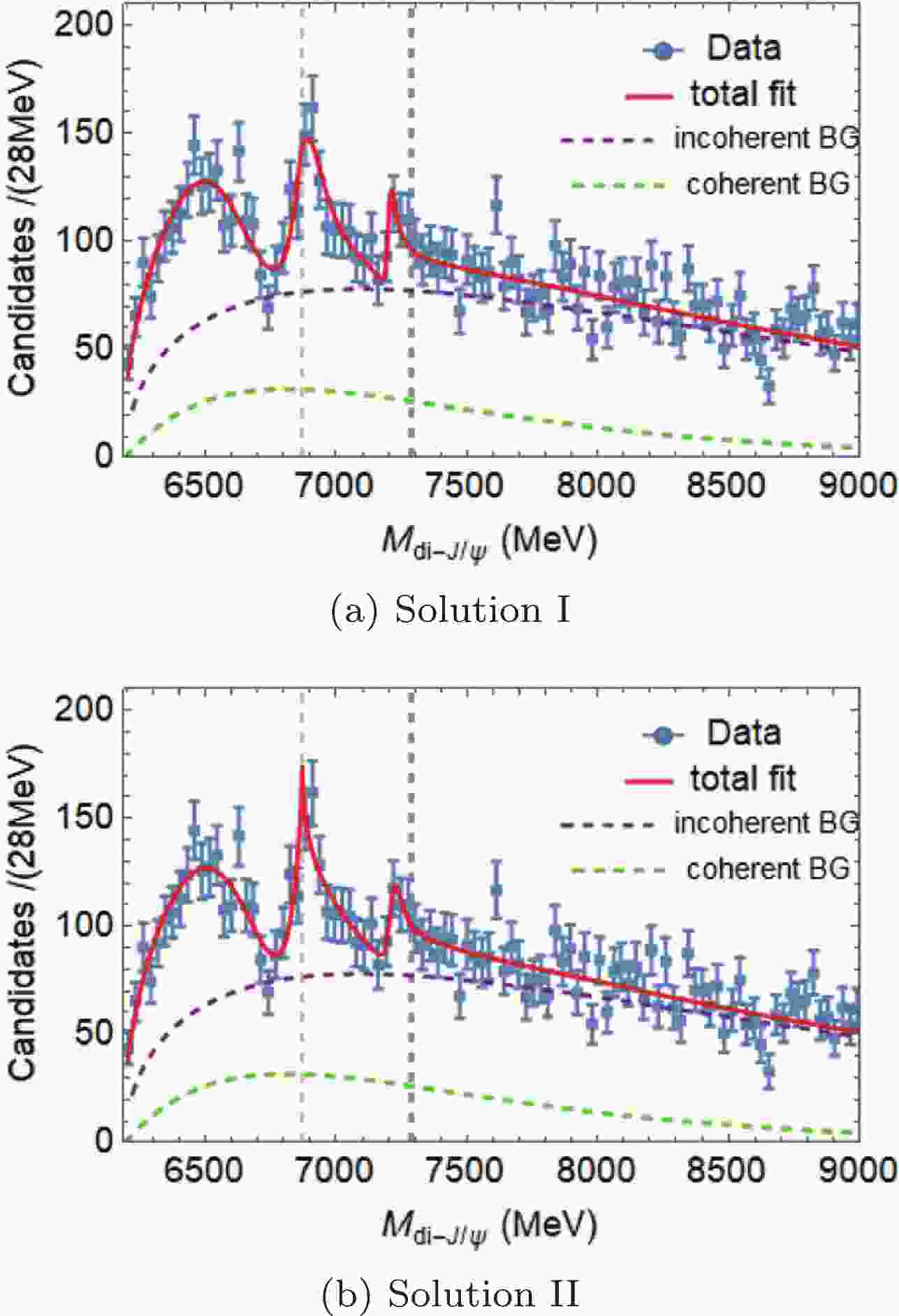
$ {\cal{M}}_{\rm{NoR}} $ describes the coherent background (BG), and the incoherent background$ {\cal{B.G.}} $ takes a parameterization similar to$ {\cal{M}}_{\rm{NoR}} $ . This background parameterization is similar to the LHCb experiment [1]. Interestingly, two sets of solutions with almost equivalent goodness of fit were found in the three cases, one of which favors that both states are confining states whereas the other supports that they are molecular bound states, using both PCR and SDFSR mentioned above. The fitting results are summarized in Table 4. Given that the fitting curves of the three cases look very similar, we only drew the fitting projections of two solutions in case I, shown in Fig. 1.Case I Case II Case III Solution I Solution II Solution I Solution II Solution I Solution II $ \chi^2 $ /d.o.f.

$ 100.1/86 $ 

$ 100.6/86 $ 

$ 97.6/86 $ 

$ 96.4/86 $ 

$ 99.2/86 $ 

$ 99.6/86 $ 

$ M_2 $ /MeV

$ 6883.3\pm100.3 $ 

$ 6881.9\pm203.2 $ 

$ 6921.5\pm147.6 $ 

$ 6850.0\pm136.7 $ 

$ 6829.8\pm113.6 $ 

$ 6850.0\pm107.8 $ 

$ g_{21} $ /MeV

$ 338.8\pm25.8 $ 

$ 1029.1\pm91.1 $ 

$ 1000.7\pm19.3 $ 

$ 1006.6\pm56.7 $ 

$ 606.5\pm18.8 $ 

$ 1005.9\pm54.1 $ 

$ g_{22} $ /MeV

$ 110.9\pm123.0 $ 

$ 1644.1\pm244.4 $ 

$ 645.9\pm56.9 $ 

$ 1683.5\pm239.1 $ 

$ 259.6\pm71.6 $ 

$ 1661.9\pm245.5 $ 

$ \phi_2 $ /rad

$ 0.7\pm1.6 $ 

$ 1.3\pm1.7 $ 

$ 3.9\pm0.9 $ 

$ 1.8\pm1.1 $ 

$ 2.7\pm1.6 $ 

$ 2.1\pm0.9 $ 

$ M_3 $ /MeV

$ 7195.1\pm212.8 $ 

$ 7150.0\pm747.5 $ 

$ 7221.1\pm172.4 $ 

$ 7165.6\pm656.0 $ 

$ 7222.2\pm182.9 $ 

$ 7169.9\pm583.2 $ 

$ g_{31} $ /MeV

$ 68.5\pm12.4 $ 

$ 151.5\pm48.6 $ 

$ 120.0\pm31.0 $ 

$ 130.4\pm52.3 $ 

$ 110.0\pm32.2 $ 

$ 127.2\pm57.7 $ 

$ g_{32} $ /MeV

$ 94.1\pm92.9 $ 

$ 832.3\pm245.7 $ 

$ 0.0004\pm151.9 $ 

$ 774.5\pm262.8 $ 

$ 0.0003\pm155.4 $ 

$ 772.7\pm 251.7 $ 

$ \phi_3 $ /rad

$ 5.5\pm0.9 $ 

$ 0.8\pm1.1 $ 

$ 4.4\pm1.9 $ 

$ 1.1\pm1.0 $ 

$ 5.2\pm1.4 $ 

$ 1.2\pm0.9 $ 

aThe remaining parameters which are not listed here are included in Table A1. Table 4. Summary of numerical results for
$ S-S $ couplings, where$ M_2 $ and$ M_3 $ are the masses of$ X(6900) $ and$ X(7200) $ , respectively;$ g_{21} $ and$ g_{31} $ are the coupling constants of$ X(6900) $ and$ X(7200) $ decaying to$ J/\psi J/\psi $ , respectively;$ g_{22} $ is the coupling constant of$ X(6900)\to J/\psi \psi(3770) $ ,$ J/\psi \psi_2(3823) $ , and$ J/\psi \psi_3(3842) $ in turn in the three cases,$ g_{32} $ is the coupling constant of$ X(7200)\to J/\psi\psi(4160) $ ;$ \phi_i\; (i = 2,3) $ is the interference phase as expressed in Eq. (3)a.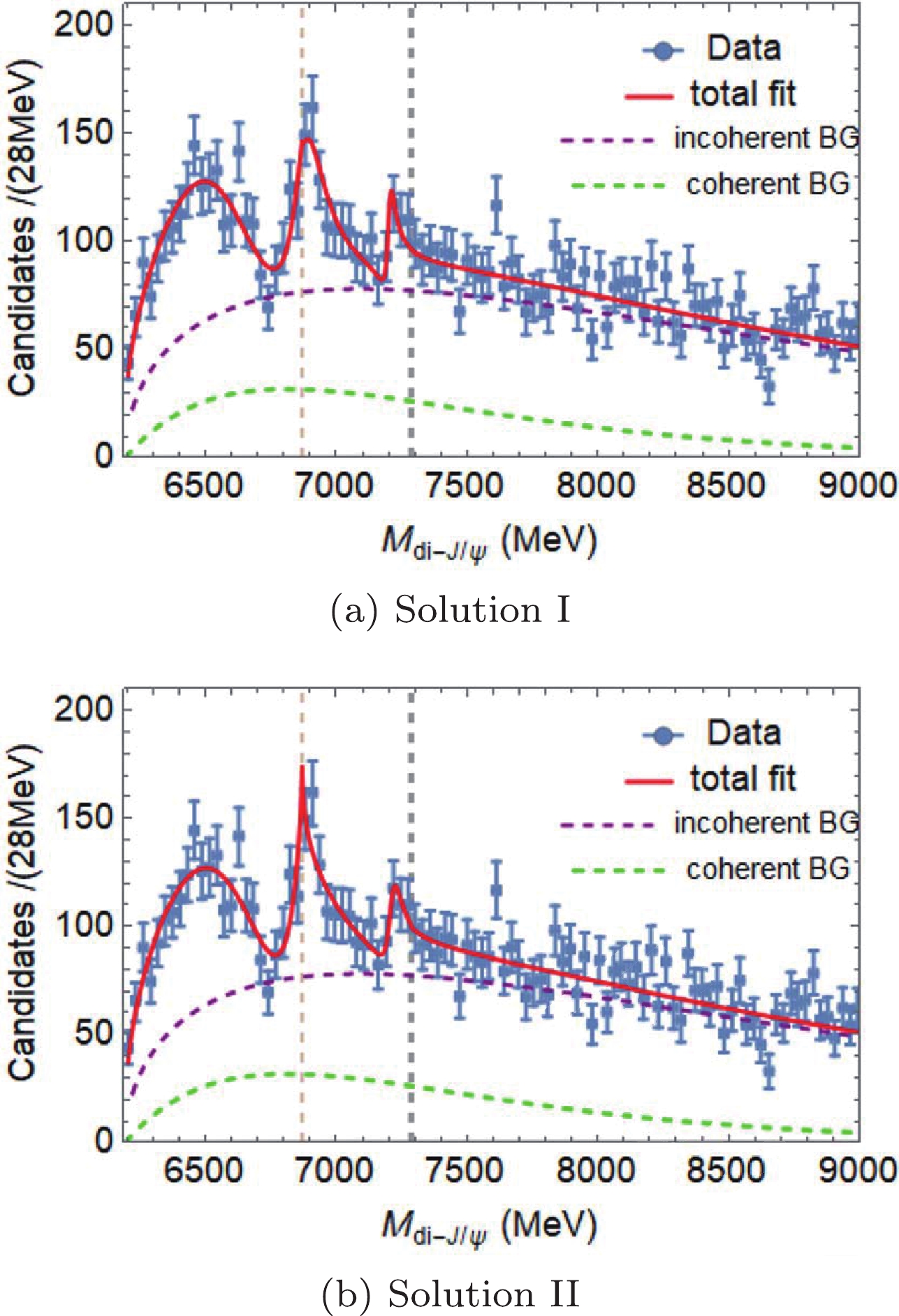
Figure 1. (color online) Fitting projections of two solutions for the
$ S-S $ couplings in Case I with$ X(6900)\to J/\psi J/\psi $ and$ J/\psi \psi(3770) $ , and$ X(7200)\to J/\psi J/\psi $ and$ J/\psi \psi(4160) $ couples, where the dots with error bars are the LHCb data [1], the red lines are the best fit, the green dashed lines show the coherent BG, the purple dashed lines are the contribution of the incoherent BG, and the vertical lines indicate the corresponding mass thresholds of$ X(6900) $ and$ X(7200) $ .Each set of the parameters can be used to determine whether the resonance structure studied in this paper is a confining state or a molecular state. The definition of Riemann sheets for two channels is listed in Table 5. The pole positions in the
$ {s} $ plane obtained by using parameters in Table 4 for all cases are summarized in Table 6. For Solution I, the fact that pole positions of$ X(7200) $ on the second and third sheets are equal in Case I and Case II indicates the$ X(7200) $ state hardly couples to the$ J/\psi \psi(4160) $ channel, whereas its pole positions in Case III manifests that it tends to be a confining state. Furthermore, it is evident for this solution in each case that the co-existence of two poles near the$ X(6900) $ threshold indicates that it might be a confining state for$ S $ -wave couplings. For Solution II in each case, the fact that only one pole is found on sheet II near the second threshold demonstrates that the two states tend to be molecular states. Thus, in case of assuming$ X(6900) $ and$ X(7200) $ to be$ J^{PC} = (0,2)^{++} $ and considering the couple channels listed in Table 1, different conclusions concerning the goodness of fit being almost equivalent are drawn. This is mainly caused by low statistics and unavailable information on other channels. Consequently, it is impossible to distinguish whether the two states are confining or molecular states under the current situation. More experimental measurements in the coupling channels,$ X(6900)\to J/\psi \psi(3770) $ ,$ J/\psi \psi_2(3823) $ ,$ J/\psi \psi_3(3842) $ ,$ \chi_{c0} \chi_{c1} $ , and$ X(7200) $ $ \to $ $ J/\psi\psi(4160) $ ,$ \chi_{c0} $ $ \chi_{c1} $ $ (3872) $ , are therefore in urgent need to clarify their nature.I II III IV $ \rho_{i1} $ 

+ − − + $ \rho_{i2} $ 

+ + − − Table 5. Definition of Riemann sheets (
$ i = 2,3 $ ).Case State Sheet II Sheet III Sol. I I $ X(6900) $ 

$ 6885.4-68.0 i $ 

$ 6874.4-80.0 i $ 

$ X(7200) $ 

$ 7202.2-16.6 i $ 

$ 7187.1-18.0 i $ 

II $ X(6900) $ 

$ 6947.6-172.0 i $ 

$ 6810.4-274.0 i $ 

$ X(7200) $ 

$ 7220.8-31.0 i $ 

$ 7220.8-31.0 i $ 

III $ X(6900) $ 

$ 6845.2-117.0 i $ 

$ 6789.2-138.0 i $ 

$ X(7200) $ 

$ 7221.9-28.0 i $ 

$ 7221.9-28.0 i $ 

Sol. II I $ X(6900) $ 

$ 6937.9-97.0 i $ 

$ 6527.3-323.0 i $ 

$ X(7200) $ 

$ 7210.7-27.5 i $ 

$ 7037.3-47.5 i $ 

II $ X(6900) $ 

$ 6933.9-111.0 i $ 

$ 6443.8-275. 0i $ 

$ X(7200) $ 

$ 7218.9-24.0 i $ 

$ 7067.9-41.5 i $ 

III $ X(6900) $ 

$ 6933.3-113.0 i $ 

$ 6452.3-275.0 i $ 

$ X(7200) $ 

$ 7221.9-23.0 i $ 

$ 7073.7-41.0 i $ 

Table 6. Summary of pole positions obtained using central values of parameters for
$ S-S $ couplings. Here, the symbol "Sol." denotes "Solution" throughout the analysis.At last, we also tested the situation in which
$ X(6900) $ couples to$ J/\psi J/\psi $ and$ J/\psi\psi(2S) $ . A solution that favors$ X(6900) $ as a confining state was found. Meanwhile, we could not find a good solution in favor of a molecular state interpretation of$ X(6900) $ . -
With the quantum numbers of the
$ P $ -wave$ J/\psi J/\psi $ pair being$ (0,1,2)^{-+} $ , coupling channel thresholds close to the two states are summarized in Table 2. From this table, the couplings can be divided into two cases:Case I:
$ X(6900)\to J/\psi J/\psi $ ,$ \chi_{c0} \chi_{c1} $ ;$ X(7200)\to J/\psi J/\psi $ ,$ \chi_{c0}\chi_{c1}(3872) $ .Case II:
$ X(6900)\to J/\psi J/\psi $ ,$ J/\psi \psi(3770) $ ;$ X(7200) \to $ $ J/\psi J/\psi $ and$ J/\psi \psi(4160) $ .By employing Eq. (3) with the threshold and barrier factors
$ n_{ij}(s) $ included, the fitting projections are shown in Fig. 2, and the corresponding numerical results are listed in Table 7. Note that the parameterization with the$ P $ -wave coupling assumption can also meet the experimental data well, with almost equivalent goodness of fit in the$ S $ -wave couplings. The pole positions in the complex$ s $ plane are listed in Table 8. Note that the method adopted in this study cannot distinguish a$ P $ -wave confining state from a$ P $ -wave molecule, given that they both contribute two pair of poles near the threshold.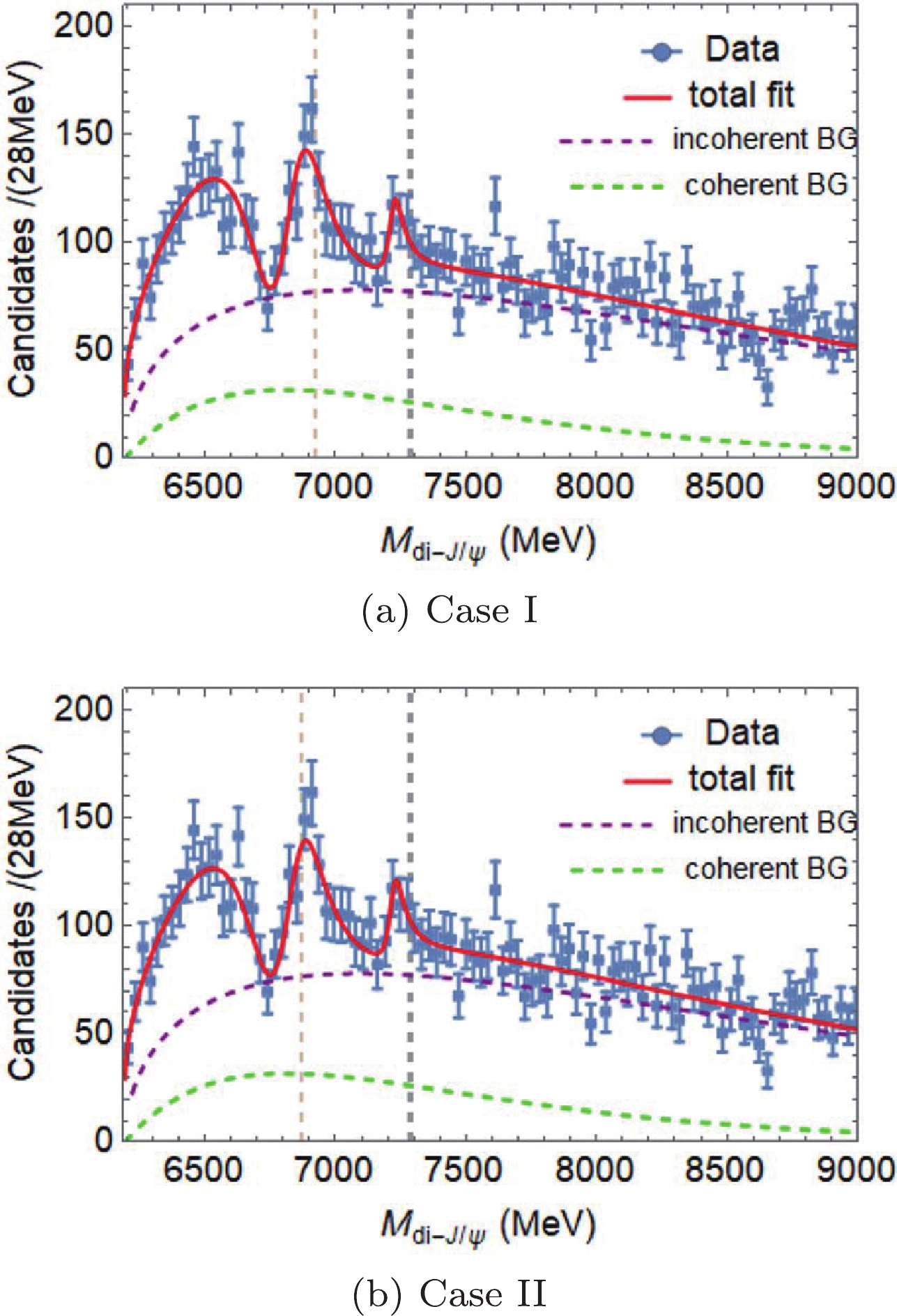
Figure 2. (color online) Fitting projections for the
$ P-P $ couplings, where Fig. (a) shows$ X(6900) $ decaying to$ J/\psi J/\psi $ and$ \chi_{c0} \chi_{c1} $ , and$ X(7200) $ to$ J/\psi J/\psi $ and$ \chi_{c0}\chi_{c1}(3872) $ , and Fig. (b) illustrates$ X(6900)\to J/\psi J/\psi $ and$ J/\psi \psi(3770) $ ,$ X(7200)\to J/\psi J/\psi $ and$ J/\psi \psi(4160) $ . Here, the descriptions of the components of the figures are similar to those of Fig. 1.Case I Case II $ \chi^2 $ /d.o.f.

$ 95.7/86 $ 

$ 95.6/86 $ 

$ M_2 $ /MeV

$ 6866.9\pm51.4 $ 

$ 6869.6\pm60.2 $ 

$ g_{21} $ /MeV

$ 4679.6\pm128.6 $ 

$ 4679.2\pm136.3 $ 

$ g_{22} $ /MeV

$ 1010.1\pm1520.1 $ 

$ 2585.2\pm1828.7 $ 

$ \phi_2 $ /rad

$ 1.7\pm1.4 $ 

$ 1.7\pm1.6 $ 

$ M_3 $ /MeV

$ 7228.2\pm50.1 $ 

$ 7229.7\pm50.7 $ 

$ g_{31} $ /MeV

$ 568.8\pm60.6 $ 

$ 569.3\pm59.8 $ 

$ g_{32} $ /MeV

$ 7105.6\pm5964.6 $ 

$ 8158.6\pm5610.5 $ 

$ \phi_3 $ /rad

$ 5.7\pm0.6 $ 

$ 5.7\pm0.6 $ 

aThe remaining parameters which are not listed here are displayed in the Table A2. Table 7. Summary of numerical results for
$ P-P $ couplings, where$ M_2 $ and$ M_3 $ are the masses of$ X(6900) $ and$ X(7200) $ , respectively;$ g_{21} $ and$ g_{31} $ are the coupling constants of$ X(6900) $ and$ X(7200) $ decaying to$ J/\psi J/\psi $ , respectively;$ g_{22} $ is the coupling constant of$ X(6900)\to\chi_{c0}\chi_{c1} $ and$ J/\psi \psi(3770) $ in the two cases,$ g_{32} $ is the coupling constant of$ X(7200)\to J/\psi\psi(4160) $ ;$ \phi_i\; (i = 2,3) $ is the interference phase as expressed in Eq. (3)a.State Sheet II Sheet III Case I $ X(6900) $ 

$ 6838.7-119.0 i $ 

$ 6840.9-113.0 i $ 

$ X(7200) $ 

$ 7220.8-31.0 i $ 

$ 7232.5-23.0 i $ 

Caes II $ X(6900) $ 

$ 6844.1-122.0 i $ 

$ 6841.2-110.5 i $ 

$ X(7200) $ 

$ 7221.4-32.0 i $ 

$ 7234.4-22.0 i $ 

Table 8. Summary of pole positions obtained using central values of parameters for the
$ P-P $ couplings. -
Owing to the limited statistics but multiple states, only two cases were considered in the analysis for the
$ S-P $ and$ P-S $ couplings:Case I (
$ S-P $ ):$ S $ -wave for$ X(6900)\to J/\psi J/\psi $ ,$ J/\psi \psi(3770) $ ;$ P $ -wave for$ X(7200) \to J/\psi J/\psi $ and$ J/\psi \psi(4160) $ .Case II (
$ P-S $ ):$ P $ -wave for$ X(6900)\to J/\psi J/\psi $ ,$ J/\psi \psi(3770) $ ;$ S $ -wave for$ X(7200) \to J/\psi J/\psi $ and$ J/\psi \psi(4160) $ .The following total amplitude is applicable for both cases,
$ |{\cal{M}}|^2 = \Bigg| \sum\limits_{i = 1}^{2} {\cal{M}}_i + {\cal{M}}_{\rm{NoR}} \Bigg|^{2} + |{\cal{M}}_3|^{2} + {\cal{B.G.}} $

(4) By employing Eq. (4) with the respective threshold and barrier factors,
$ n_{ij}(s) $ included, the fitting projections are similar to Fig. 1. Two sets of solutions with almost equivalent goodness of fit were found in Case I. In comparison, only one solution in favor of a molecular interpretation of$ X(7200) $ was found in Case II. The pole positions in the complex$ s $ plane are summarized in Table 9. Based on PCR, it may be concluded that Solution I favors$ X(6900) $ as a confining state and Solution II supports that it is a molecular bound state.Sol. State Sheet II Sheet III Case I I $ X(6900) $ 

$ 6901.0-32.6 i $ 

$ 6884.4-61.7 i $ 

$ X(7200) $ 

$ 7196.2 -19.5 i $ 

$ 7200.8-17.4 i $ 

II $ X(6900) $ 

$ 6894.8-65.3 i $ 

$ - $ 

$ X(7200) $ 

$ 7097.8-17.6 i $ 

$ 7128.1-14.0 i $ 

Case II $ X(6900) $ 

$ 6900.5-14.5 i $ 

$ 6900.3-15.2 i $ 

$ X(7200) $ 

$ 7362.2-67.9 i $ 

$ - $ 

Table 9. Summary of pole positions obtained using central values of parameters for
$ S-P $ and$ P-S $ couplings. -
Concerning
$ S $ -waves, SDFSR can be utilized to provide insights into the nature of the$ X(6900) $ state. Ref. [27] pointed out that the spectrum density function$ \omega(E) $ near threshold can be calculated by using the non-relativistic$ S $ -wave Flatté parameterization, and the renormalization constant$ {\cal{Z}} $ can be obtained, which represents the probability of finding the confining particle in the continuous spectrum: the greater the tendency of$ {\cal{Z}} $ to$ 1 $ , the more confining is the state. On the other hand, if$ {\cal{Z}} $ tends to 0, the state tends to be molecular.Using a form similar to that in Refs. [25,27-30], the spectrum density function of a near-threshold channel can be expressed as
$ \omega(E) = \frac{1}{2\pi}\frac{\tilde{g}\sqrt{2\mu E}\theta(E)+\tilde{\Gamma}_{0}}{\left|E-E_{f}+\dfrac{\rm i}{2}\tilde{g}\sqrt{2\mu E}\theta(E)+\dfrac{\rm i}{2}\tilde{\Gamma}_0\right|^2}, $

(5) where
$ E\; (E_f) = \sqrt{s}\; (M)-m_{th} $ is the energy difference between the center-of-mass energy (resonant state) and the open-channel threshold,$ \mu $ is the reduced mass of the two-body final states of the channel,$ \theta $ is the step function,$ \tilde{g} = 2g/m_{th} $ is the dimensionless coupling constant of the concerned coupling mode, and$ \tilde{\Gamma_0} $ is the constant partial width for the remaining couplings, which mainly contains the distant channels (the$ J/\psi J/\psi $ process in this analysis).By integrating Eq. (5), the probability of finding an "elementary" particle in the continuous spectrum can be obtained:
$ {\cal{Z}} = \int_{E_{\min}}^{E_{\max}}\omega(E){\rm d}E. $

(6) The integral interval takes
$ E_f $ as the central value. It is pointed out in Ref. [30] that the integration interval needs to cover the threshold of the coupling channel. Given that the$ X(7200) $ state is of no significance ($ \sim3\; \sigma $ reported in the LHCb experiment [1]), only the$ {\cal{Z}} $ values of$ X(6900) $ , as listed in Table 1, are calculated. Expanding$ \omega(E) $ near the threshold of each channel, and bringing$ X(6900) $ 's mass$M^{\rm pole}_2$ and width$\Gamma^{\rm pole}_2$ extracted from the second Riemann sheet in Table 6, one can obtain the corresponding$ {\cal{Z}} $ value, where$ \tilde{\Gamma_0} = \Gamma_{21}(M^{\rm{pole}}_2) $ (see also Eq. (2)). The numerical$ {\cal{Z}} $ values are summarized in Table 10, where the interval$ [E_f-\Gamma,E_f+\Gamma] $ covers all thresholds of the calculated channels. The$ {\cal{Z}} $ values in Solution I are all slightly less than 50% in this interval, but rapidly exceeds 50% in larger integral intervals. Hence$ X(6900) $ may be considered as a confining state in Solution I. For Solution II, the$ {\cal{Z}} $ values are much smaller than 50% in the interval$ [E_f-\Gamma,E_f+\Gamma] $ , and also less than 50% in the interval$ [E_f-2\Gamma,E_f+2\Gamma] $ . This suggests that the$ X(6900) $ state is more likely a molecular state in Solution II. As a conclusion, the nature of$ X(6900) $ is consistently drawn from both PCR and SDFSR based on the current limited data. Hence, we were not able to distinguish whether it is a confining state or a molecular bound state.Case $ [E_f-\Gamma,E_f+\Gamma] $ 

$ [E_f-2\Gamma,E_f+2\Gamma] $ 

Sol. I I 0.459 0.671 II 0.379 0.592 III 0.468 0.681 Sol. II I 0.184 0.344 II 0.243 0.418 III 0.259 0.438 Table 10. Summary of
$ {\cal{Z}} $ values for the$ S-S $ couplings of$ X(6900) $ . -
In this analysis, the channels
$ J/\psi \psi(3770) $ ,$ J/\psi \psi_2(3823) $ ,$ J/\psi \psi_3(3842) $ , and$ \chi_{c0} \chi_{c1} $ [$ J/\psi\psi(4160) $ and$ \chi_{c0}\chi_{c1}(3872) $ ] close to the threshold of$ X(6900) $ [$ X(7200) $ ] were selected to study their couplings. Fitting to recent LHCb data through Flatté-like parameterization with momentum-dependent partial widths, we found that the lowest state in the di-$ \psi $ mass spectrum with the same quantum numbers as$ X(6900) $ is essential to describe the extremely deep dip below 6800 MeV by destructive interference. The amplitude poles in the complex$ s $ plane were obtained. For the$ S $ -wave$ J/\psi J/\psi $ couplings, PCR and SDFSR were imposed to determine whether the structures are confining states (bound by color force) or molecular states. The two approaches provide consistent conclusions: both confining and molecular states are possible, or the nature of the two states cannot be distinguished if only the di-$ J/\psi $ experimental data with current statistics are available. It is also discussed in Ref. [12] that the current experimental data are not enough to provide a definitive conclusion on the nature of$ X(6900) $ . In addition, the$ X(6900)\to J/\psi \psi(2S) $ coupling with the threshold far away from$ X(6900) $ 's mass was taken into account. Our results do not favor the$ X(6900) $ structure as a$ J/\psi \psi(2S) $ molecular state. In the future, we are hoping to obtaine more experimental data and more decay channels to clarify the nature of$ X(6900) $ and$ X(7200) $ as well as determine their$ J^{PC} $ quantum numbers. Reasonably, we suggest that experiments measure$ X(6900)\to $ $ J/\psi \psi(3770) $ ,$ J/\psi \psi_2(3823) $ ,$ J/\psi \psi_3(3842) $ , and$ \chi_{c0} \chi_{c1} $ ; and$ X(7200)\to $ $ J/\psi $ $ \psi(4160) $ ,$ \chi_{c0} $ $ \chi_{c1}(3872) $ decays, which are expected to be available in LHCb, Belle-II, CMS and other (future) experiments. -
The remaining parameters which are not listed in Sec. II are presented below. The parameter values for
$ S-S $ and$ P-P $ couplings are displayed in Table A1 and Table A2, respectively.Case I Case II Case III Solution I Solution II Solution I Solution II Solution I Solution II $ g_1 $ /MeV2

$ (34.5\pm 3.5)\times 10^6 $ 

$ (56.2\pm 5.6)\times 10^6 $ 

$ (35.0\pm 3.6)\times 10^6 $ 

$ (37.2\pm 4.3)\times 10^6 $ 

$ (57.8\pm 4.0)\times 10^6 $ 

$ (28.2\pm 3.8)\times 10^6 $ 

$ \phi_1 $ /rad

$ 3.6\pm 0.1 $ 

$ 3.6\pm 0.1 $ 

$ 5.8\pm 0.1 $ 

$ 3.8\pm 0.1 $ 

$ 4.8\pm 0.1 $ 

$ 3.9\pm 0.1 $ 

$ M_1 $ /MeV

$ 6621.6\pm 60.0 $ 

$ 6726.8\pm 164.0 $ 

$ 6741.0\pm 59.1 $ 

$ 6683.3\pm 155.9 $ 

$ 6737.0\pm 78.5 $ 

$ 6671.0\pm 101.6 $ 

$ g_{11} $ /MeV

$ 540.9\pm 55.6 $ 

$ 719.7\pm 66.0 $ 

$ 296.4\pm 22.2 $ 

$ 543.3\pm 53.8 $ 

$ 412.1\pm 33.4 $ 

$ 450.0\pm 51.2 $ 

$ g_{2} $ /MeV2

$ (11.9\pm 0.8)\times 10^6 $ 

$ (40.2\pm 5.6)\times 10^6 $ 

$ (71.3\pm 4.7)\times 10^6 $ 

$ (32.4\pm 3.3)\times 10^6 $ 

$ (35.0\pm 5.6)\times 10^6 $ 

$ (29.0\pm 2.9)\times 10^6 $ 

$ g_{3} $ /MeV2

$ (2.3\pm 0.3)\times 10^6 $ 

$ (2.0\pm 0.6)\times 10^6 $ 

$ (1.8\pm 0.4)\times 10^6 $ 

$ (1.6\pm 0.5)\times 10^6 $ 

$ (1.6\pm 0.4)\times 10^6 $ 

$ (1.6\pm 0.5)\times 10^6 $ 

Table A1. Parameter values for
$ S-S $ coupling. Other parameter values are listed in Table 4.Case I Case II $ g_1 $ /MeV2

$ (41.7\pm 3.1)\times 10^6 $ 

$ (41.7\pm 3.1)\times 10^6 $ 

$ \phi_1 $ /rad

$ 4.1\pm 0.1 $ 

$ 4.0\pm 0.1 $ 

$ M_1 $ /MeV

$ 6753.8\pm 60.7 $ 

$ 6748.7\pm 85.5 $ 

$ g_{11} $ /MeV

$ 402.8\pm 33.7 $ 

$ 414.6\pm 34.1 $ 

$ g_2 $ /MeV2

$ (74.3\pm 8.9)\times 10^6 $ 

$ (72.2\pm 8.4)\times 10^6 $ 

$ g_3 $ /MeV2

$ (8.0\pm 0.6)\times 10^6 $ 

$ (7.9\pm 0.6)\times 10^6 $ 

Table A2. Parameter values for
$ P-P $ coupling. Other parameter values are listed in Table 7.For
$ S-P $ coupling, in which$ X(6900) $ couples to$ S $ -wave di-$ J/\psi $ and$ J/\psi\psi(3770) $ , and$ X(7200) $ couples to$ P $ -wave di-$ J/\psi $ and$ J/\psi\psi(4160) $ , the parameter values are listed in Table A3.Sol. I Sol. II $ \chi^2/d.o.f. $ 

98.2/87 103.3/87 $ g_1 $ /MeV2

$ (19.9\pm 4.2)\times 10^{6} $ 

$ (41.8\pm 5.4)\times 10^6 $ 

$ \phi_1 $ /rad

$ 3.4\pm 0.1 $ 

$ 3.3\pm 0.1 $ 

$ M_1 $ /MeV

$ 6599.5\pm 24.4 $ 

$ 6670.7\pm 33.9 $ 

$ g_{11} $ /MeV

$ 462.4\pm 91.2 $ 

$ 752.9\pm 91.7 $ 

$ g_2 $ /MeV2

$ (50.0\pm 5.5)\times 10^6 $ 

$ (25.0\pm 1.3)\times 10^6 $ 

$ \phi_2 $ /rad

$ 2.0\pm 0.5 $ 

$ 1.1\pm0.2 $ 

$ M_2 $ /MeV

$ 6896.1\pm 27.4 $ 

$ 6800.0\pm 28.7 $ 

$ g_{21} $ /MeV

$ 215.8\pm 48.2 $ 

$ 1000.0\pm 41.0 $ 

$ g_{22} $ /MeV

$ 250.0\pm 117.9 $ 

$ 2550.0\pm 587.5 $ 

$ g_3 $ /MeV2

$ (7.6\pm 1.6)\times 10^6 $ 

$ (7.4\pm 2.9)\times 10^6 $ 

$ M_3 $ /MeV

$ 7199.0 \pm 102.9 $ 

$ 7115.3\pm 263.8 $ 

$ g_{31} $ /MeV

$ 400.0\pm 106.3 $ 

$ 400.0\pm 127.5 $ 

$ g_{32} $ /MeV

$ 1463.7\pm 257.6 $ 

$ 3424.8\pm 351.1 $ 

Table A3. Parameter values for
$ S-P $ coupling.For
$ P-S $ coupling, in which$ X(6900) $ couples to$ P $ -wave di-$ J/\psi $ and$ J/\psi\psi(3770) $ , and$ X(7200) $ couples to$ S $ -wave di-$ J/\psi $ and$ J/\psi\psi(4160) $ , the parameter values are shown in Table A4.$ \chi^2/d.o.f. $ 

97.23/87 $ g_1 $ /MeV2

$ (29.5\pm 2.8)\times 10^{6} $ 

$ \phi_1 $ /rad

$ 4.4\pm 0.2 $ 

$ M_1 $ /MeV

$ 6742.8\pm 17.9 $ 

$ g_{11} $ /MeV

$ 1000.0\pm 80.8 $ 

$ g_2 $ /MeV2

$ (20.0\pm 2.5)\times 10^6 $ 

$ \phi_2 $ /rad

$ 2.3\pm 0.5 $ 

$ M_2 $ /MeV

$ 6900.8\pm 25.9 $ 

$ g_{21} $ /MeV

$ 550.0\pm 31.6 $ 

$ g_{22} $ /MeV

$ 250.0\pm 40.6 $ 

$ g_3 $ /MeV2

$ (31.2\pm 10.2)\times 10^6 $ 

$ M_3 $ /MeV

$ 7255.8 \pm 115.4 $ 

$ g_{31} $ /MeV

$ 1377.9\pm 505.0 $ 

$ g_{32} $ /MeV

$ 3999.7\pm 2352.5 $ 

Table A4. Parameter values for
$ P-S $ coupling.In addition, the parameters for both coherent and incoherent background terms, which were obtained from fitting to the mass spectrum without the signal amplitude, were fixed throughout default fitting to reduce the uncertainty of the multiple interference. Regarding the coherent background,
$ c_0 = 20.9 $ and$ c_1 = -6.9\times 10^{-4} $ (MeV−1). Concerning the incoherent background, which takes a form similar to the coherent background, it has two parameters:$ a_0 = 240.7 $ ,$ a_1 = -4.5\times 10^{-4} $ (MeV−1).
Some remarks on X(6900)
- Received Date: 2021-05-21
- Available Online: 2021-10-15
Abstract: The analysis of the LHCb data on


 DownLoad: