


 Abstract
 HTML
HTML Reference
 Related
 PDF
PDF


-
Dilaton gravity [1-3] has received considerable attention within the community for its great physical significance. Firstly, it serves as the low energy limit of string theory, as one can recover Einstein gravity with a non-minimally coupled dilaton field and other fields in the low energy limit. Secondly, its action consists of one or more Liouville-type potentials. These potentials can be created by spacetime supersymmetry breaking in ten dimensions. Additionally, it has been reported that the dilaton field may affect both the casual structure and thermodynamic properties of black holes. Due to the physical importance of this, various black hole solutions have been presented and their thermodynamic properties discussed [1-56]. Interestingly, it was also put forward in Refs. [14-16] that the cosmological constant is found to be coupled to Liouville-type potential in the dilaton theory.
Among these solutions, a class of
$ (n+1) $ -dimensional topological black hole solutions were obtained [26] in Einstein-Maxwell-dilaton theory, which are neither asymptotically flat nor anti-de Sitter. The thermodynamic properties of these black holes were carefully analyzed. Moreover, the effect of the dilaton field on thermal stability was detailed [26].$ P-V $ criticality was investigated in Refs. [27, 28]. Provided the coupling constant of dilaton gravity is less than one, the critical values of relevant physical quantities are physical [28]. Ref. [29] investigated phase transitions and thermodynamic geometry, while Ref. [30] provided further details on the existence of a zeroth-order phase transition. The two point correlation function and the entanglement entropy of dilaton black holes were studied by one of the authors [31], providing an alternative perspective to observe the critical phenomena in dilaton black holes. Additionally, with Ruppeiner geometry, Ref. [32] attempted to provide a microscopic explanation for the phase transitions of charged dilatonic black holes.Although many attempts have been made, the dynamic phase transition of this typical class of dilaton black hole solutions proposed in Ref. [26] and the related kinetics remain inadequately explained. Therefore, the motivation for this paper was to obtain this “missing puzzle piece” concerning the phase transition of charged dilaton black holes. The dynamic phase transition of black holes has emerged as a popular topic since the recent creative works reporting the kinetics of the Hawing-Page phase transition [57] and the van der Waals-like phase transition [58]. For the latter, the transition between the large black hole and the small black hole due to thermal fluctuation can be viewed as stochastic process, which can then be analyzed via the Fokker-Planck equation [58]. Subsequently, dynamic phase transitions of Gauss-Bonnet black holes [59-61] and charged AdS black holes surrounded by quinteness dark energy [62] were investigated. Furthermore, it was suggested in a recent study [63] that the turnover of the kinetics can be used to investigate the microstructure of black holes. It is of significant interest to generalize these studies to dilaton black holes considering the physical importance of dilaton gravity, as stated in the first paragraph. It is expected that this will reveal novel features of the dynamic phase transition of black holes.
This paper is organized as follows. Sec. II is devoted to a short review of the thermodynamic properties of charged dilaton black holes. Sec. III investigates the dynamic phase transition of charged dilaton black holes. The first passage process for the phase transition of charged dilaton black holes is explored in Sec. IV. Finally, conclusions are presented in Sec. V.
-
The Einstein-Maxwell-Dilaton action in
$ (n+1) $ -dimensional spacetime reads [8]$ \begin{aligned}[b] S =& \frac{1}{16\pi}\int {\rm d}^{n+1}x \sqrt{-g}\Bigg(\mathcal{R}-\frac{4}{n-1}(\nabla \Phi)^2-V(\Phi)\\&-{\rm e}^{-4\alpha \Phi/(n-1)}F_{\mu\nu}F^{\mu\nu}\Bigg), \end{aligned} $

(1) where
$ \mathcal{R} $ ,$ \Phi $ , and$ F_{\mu\nu} $ denote the Ricci scalar curvature, dilaton field, and electromagnetic field tensor, respectively. The parameter$ \alpha $ describes the strength of the coupling between the electromagnetic and dilaton fields.To obtain a solution, one must adopt a specific form of the potential of the dilaton field
$ V(\Phi) $ ; in this case,$ V(\Phi) = $ $ 2\Lambda_0{\rm e}^{2\zeta_0\Phi}+2\Lambda {\rm e}^{2\zeta\Phi} $ [8, 17, 18, 26]. Note that if the power-law Maxwell field is considered [22], an additional term should be added to the above potential.One can take the general form of the metric as [26]
$ {\rm d}s^2 = -f(r){\rm d}t^2+\frac{1}{f(r)}{\rm d}r^2+r^2R^2(r)h_{ij}{\rm d}x^i{\rm d}x^j, $

(2) where
$ h_{ij}{\rm d}x^i{\rm d}x^j $ corresponds to an$ (n-1) $ -dimensional hypersurface with constant scalar curvature$ (n-1)(n-2)k $ , where k can be taken as$ -1,\;0,\;1 $ , corresponding to hyperbolic, flat, and spherical constant curvature hypersurfaces, respectively.Employing the ansatz
$ R = {\rm e}^{2\alpha\Phi/(n-1)} $ , the solution can be derived [26] as$ \begin{aligned}[b] f(r) =& -\frac{k(n-2)(1+\alpha^2)^2b^{-2\gamma}r^{2\gamma}}{(\alpha^2-1)(\alpha^2+n-2)}-\frac{m}{r^{(n-1)(1-\gamma)-1}}\\&+\frac{2\Lambda b^{2\gamma}(1+\alpha^2)^2r^{2(1-\gamma)}}{(n-1)(\alpha^2-n)} \\& +\frac{2q^2(1+\alpha^2)^2b^{-2(n-2)\gamma}r^{2(n-2)(\gamma-1)}}{(n-1)(n+\alpha^2-2)},\end{aligned}$

(3) $ \Phi(r) = \frac{(n-1)\alpha}{2(\alpha^2+1)}\ln \left(\frac{b}{r}\right), $

(4) where b is an arbitrary constant and
$ \gamma $ is related to$ \alpha $ by$ \gamma = \alpha^2/(\alpha^2+1) $ . The coefficients in the expression of$ V(\Phi) $ are [26]$ \Lambda_0 = \frac{k(n-1)(n-2)\alpha^2}{2b^2(\alpha^2-1)},\;\;\;\zeta_0 = \frac{2}{\alpha(n-1)},\;\;\;\;\zeta = \frac{2\alpha}{n-1}.$

(5) The mass, charge, Hawking temperature, and entropy are obtained as [26, 27]
$ M = \frac{b^{(n-1)\gamma}(n-1)\omega_{n-1}m}{16\pi (\alpha^2+1)} , $

(6) $ Q = \frac{\omega_{n-1}q}{4\pi}, $

(7) $\begin{aligned}[b] T=& \frac{-(1+\alpha^2)}{2\pi(n-1)}\Bigg[\frac{k(n-2)(n-1)}{2b^{2\gamma}(\alpha^2-1)}r_+^{2\gamma-1}+\Lambda b^{2\gamma} r_+^{1-2\gamma}\\&+q^{2}b^{-2(n-2)\gamma}r_+^{(2n-3)(\gamma-1)-\gamma}\Bigg], \end{aligned} $

(8) $ S = \frac{\omega_{n-1}b^{(n-1)\gamma}r_+^{(n-1)(1-\gamma)}}{4}. $

(9) where the parameter
$ m $ can be derived via$ f(r_+) = 0 $ .By considering the conditions that the electric potential
$ A_t $ should be finite at infinity and the parameter m should vanish at spacial infinity, the restrictions on$ \alpha $ for dilaton black holes coupled with the power-law Maxwell field were obtained [22] as$ 0\leqslant\alpha^2<n-2 $ for the case where$ \dfrac{1}{2}<p<\dfrac{n}{2} $ , and as$ 2p-n<\alpha^2<n-2 $ for the case where$ \dfrac{n}{2}<p<n-1 $ , where p describes the nonlinearity of the electromagnetic field. For the Maxwell field considered here,$ p = 1 $ , reducing the corresponding restriction to$ 0\leqslant\alpha^2<n-2 $ . -
To investigate the dynamic phase transition of charged dilaton black holes, we introduce the “Gibbs free energy landscape” and define the corresponding Gibbs free energy
$ G_{\rm L} $ as$ G_{\rm L} = H-T_{\rm E}S $ . Here,$ T_{\rm E} $ denotes the temperature of the ensemble. Via Eqs. (6) and (9),$ G_{\rm L} $ of the dilaton black hole is calculated as$ \begin{aligned}[b]G_{\rm L} =& \frac{\omega_{n-1}b^{(n-1)\gamma}r_+^{n-2+(1-n)\gamma}}{16\pi}\Bigg\{\Bigg[\frac{2b^{-2(n-2)\gamma} q^2r_+^{2(n-2)(\gamma-1)}}{(n-1)(\alpha^2+n-2)}\\&-\frac{k(n-2)b^{-2\gamma}r_+^{2\gamma}}{(\alpha^2-1)(\alpha^2+n-2)}+\frac{16\pi P b^{2\gamma}r_+^{2(1-\gamma)}}{(n-1)(n-\alpha^2)}\Bigg] \\& \times(n-1)(1+\alpha^2)-4\pi r_+T_{\rm E}\Bigg\}, \end{aligned} $

(10) where we have introduced the extended phase space and set the thermodynamic pressure as
$ P = -\Lambda/8\pi $ .To observe the behavior of
$ G_{\rm L} $ $ G_{\rm L} $ it is plotted for various temperatures in Figs. 1(b)-1(f). We chose five characteristic temperatures, namely,$ T_1 $ ,$ T_2 $ ,$ T_3 $ ,$ T_4 $ , and$ T_5 $ . From Fig.1(a), we observe that$ T_1 $ and$ T_5 $ each correspond to a single phase,$ T_2 $ and$ T_4 $ correspond to three phases, and$ T_3 $ corresponds to two phases (one being a coexistent phase). All phases are denoted by black dots in Fig. 1. When$ T_{\rm E} = T_1 $ and$ T_{\rm E} = T_5 $ , there is only one local minimum (forming one well in the curve). For$ T_{\rm E} = T_2 $ and$ T_{\rm E} = T_4 $ , there are two local minimums and one local maximum (leading to two wells of different depths). For the case of$ T_{\rm E} = T_3 $ , there are two local minimum points (denoting the stable black hole phases) and one local maximum point (denoting the unstable black hole phase), that is, there are two wells also in the curve. However, in contrast to the$ T_{\rm E} = T_2 $ and$ T_{\rm E} = T_4 $ cases, these wells have the same depth. Therefore, Fig. 1(d) represents the phase transition between the small black hole and large black hole.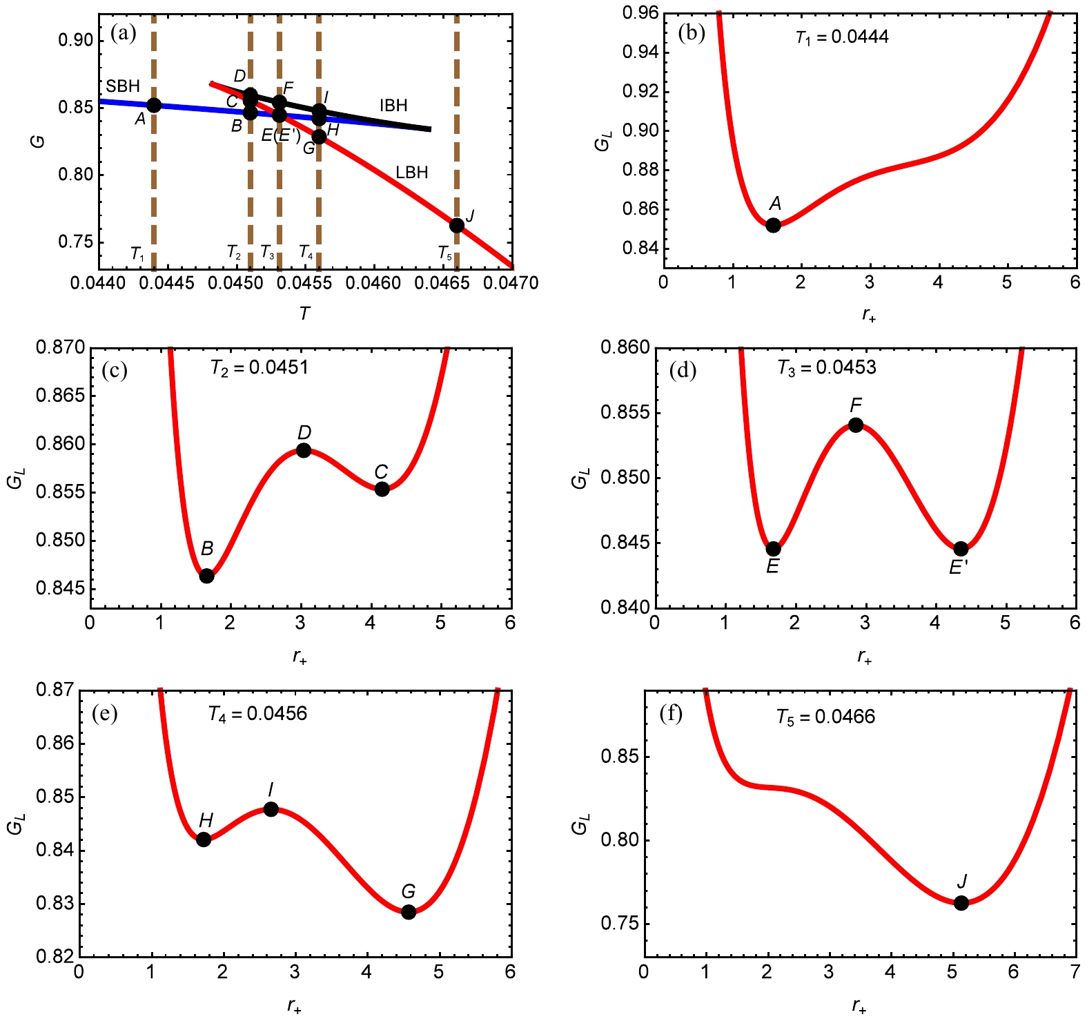
Figure 1. (color online)
$ \alpha = 0.2 $ and$ P = 0.003 $ . (a)$ G-T $ , (b)$ G-r_{+} $ for$ T_{1} = 0.0444 $ , (c)$ G-r_{+} $ for$ T_{2} = 0.0451 $ , (d)$ G-r_{+} $ for$ T_{3} = 0.0453 $ , (e)$ G-r_{+} $ for$ T_{4} = 0.0456 $ , and (f)$ G-r_{+} $ for$ T_{5} = 0.0466 $ .Based on
$ G_{\rm L} $ , we can utilize the following Fokker-Planck equation [64-68] to investigate the probabilistic evolution of the black hole after the thermal fluctuation,$ \frac{\partial \rho(r,t)}{\partial t} = D\frac{\partial}{\partial r}\left\{{\rm e}^{-\beta G_{\rm L}(T,P,r)}\frac{\partial}{\partial r}\left[{\rm e}^{\beta G_{\rm L}(T,P,r)}\rho(r,t)\right]\right\}, $

(11) where
$ \rho(r,t) $ denotes the probability distribution. Additionally, the parameter$ \beta = \dfrac{1}{k_{\rm B} T} $ incorporates$ k_{\rm B} $ as the Boltzman constant, and the diffusion coefficient$ D = \dfrac{k_{\rm B} T}{\zeta} $ incorporates$ \zeta $ , which denotes the dissipation coefficient. Without loss of generality,$ \zeta $ and$ k_{\rm B} $ can be set to one. For conciseness, we employ r to replace the notation$ r_+ $ for the black hole horizon radius here and hereafter.Before solving the above equation, the boundary condition and the initial condition must first be imposed. The initial condition can be chosen as a Gaussian wave packet located at the small and large dilaton black hole states, respectively. Namely,
$ \rho(r,0) = \dfrac{1}{\sqrt{\pi}a}{\rm e}^{-(r-r_{{\rm l(s)}})^2/a^2} $ , with$ r_{\rm l} $ and$ r_{\rm s} $ denoting the horizon radius of the large and small dilaton black holes, respectively, and a denoting the width of Gaussian wave packet. In this study, we set$ a = 0.1 $ .There are several types of boundary conditions, such as the reflecting boundary condition, absorbing boundary condition, and periodic boundary condition. Here, as
$ G_{\rm L} $ is not periodic, the periodic boundary condition is not considered. To investigate the dynamic phase transition of black holes, we consider the reflecting boundary condition and the absorbing boundary condition. The former condition can ensure the normalization of$ \rho $ . This can be considered as$ \beta G'(r)\rho(r,t)+\rho'(r,t)\big|_{r = r_0} = 0 $ , while the absorbing boundary condition can be considered as$ \rho(r_m,t) = 0 $ (the meaning of$ r_m $ is discussed in the next paragraph).We numerically solve Eq. (11), constrained by both the initial condition and the reflecting boundary condition. Fig. 2 shows the time evolution of the probability distribution
$ \rho(r,t) $ of charged dilaton AdS black holes, where the thermodynamic pressure was chosen as$ P = 0.003 $ . For the top, middle, and bottom rows of Fig. 2, the values of parameter$ \alpha $ , which characterizes the strength of coupling between the electromagnetic field and the dilaton field, were chosen as 0.4, 0.2, and 0, respectively, to compare the effect of dilaton gravity on the probability evolution.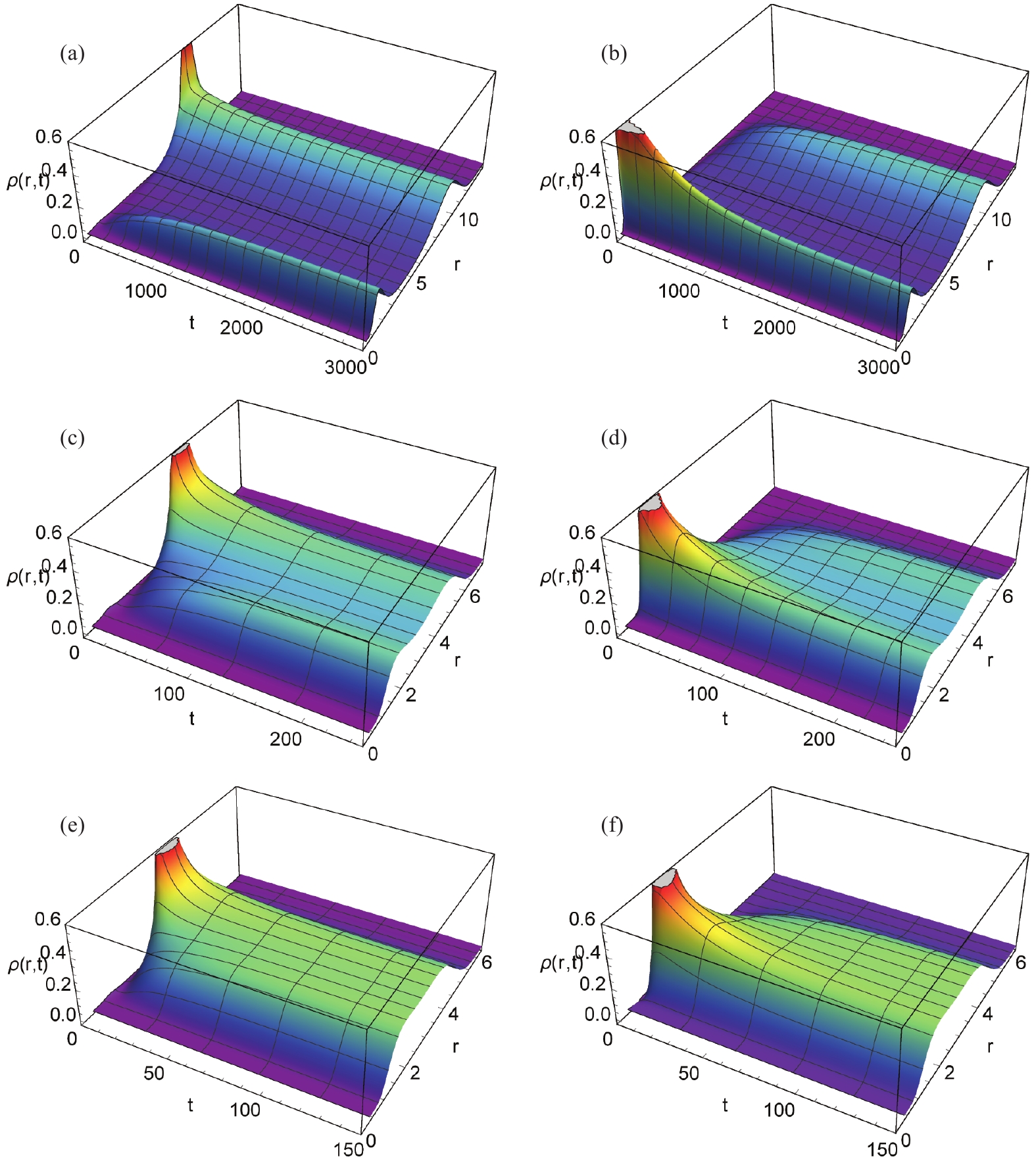
Figure 2. (color online) Time evolution of
$ \rho(r,t) $ for charged dilaton black hole with$ b = 1, \;q = 1, \;P = 0.003 $ . (a)$ \alpha = 0.4 $ , (b)$ \alpha = 0.4 $ (c)$ \alpha = 0.2$ , (d)$ \alpha = 0.2 $ (e)$ \alpha = 0$ , and (f)$ \alpha = 0 $ . For (a), (c), and (e), the initial condition was chosen as a Gaussian wave packet located at the large dilaton black hole state, while for (b), (d), and (f), the initial condition was chosen as a Gaussian wave packet located at the small dilaton black hole state.For Figs. 2(a), (c), and (e), the initial condition was chosen as a Gaussian wave packet located at the large dilaton black hole state. This is reflected in the graphs, as the initial peak of
$ \rho(r,t) $ corresponds to the radius of the large dilaton black hole. With time evolution, the initial peak decreases, while the peak corresponding to the radius of the small dilaton black hole increases. Eventually, these two peaks reach a stationary distribution in which they appear equal to each other. This demonstrates the dynamic process of the large dilaton black hole evolving into the small dilaton black hole. Therefore, the left three graphs correspond to the case where the large dilaton black hole evolves dynamically into the small dilaton black hole.In contrast, the initial condition for Figs. 2(b), (d), and (f) was chosen as a Gaussian wave packet located at the small dilaton black hole state. The initial peak located at the small dilaton black hole decays over time, while the peak corresponding to the radius of the large dilaton black hole grows. Eventually, these two peaks approach a stationary distribution. Therefore, the right three graphs of Fig. 2 correspond to the case where the small dilaton black hole evolves dynamically into the large dilaton black hole.
The effect of dilaton gravity can be observed by comparing the top two graphs (
$ \alpha = 0.4 $ ) to the middle two graphs ($ \alpha = 0.2 $ ) and the bottom two graphs ($ \alpha = 0 $ ) in Fig. 2. Firstly, the difference in horizon radius between the large and small dilaton black holes increases with the parameter$ \alpha $ . Secondly, with increasing$ \alpha $ , the system requires more time to reach a stationary distribution. Finally, the greater the overlap of the two waves, the lesser the amount of time taken for the phase transition, as it is much easier for the phase transition to take place if the two phases are more similar.Figure 3 provides a complementary, more quantitative picture of the time evolution of
$ \rho(r_{\rm l},t) $ and$ \rho(r_{\rm s},t) $ . The effect of the dilaton gravity is quite obvious. It is observed that for a larger$ \alpha $ , the phase transition is more gradual. This can be explained by the analysis in Table 1; the larger the value of$ \alpha $ , the deeper the well of Gibbs free energy. Moreover, the final values of$ \rho(r_{\rm l},t) $ and$ \rho(r_{\rm s},t) $ vary with$ \alpha $ . The values can be read from the graph, with 0.229 for$ \alpha = 0.4 $ , 0.250 for$ \alpha = 0.2 $ , and 0.297 for$ \alpha = 0 $ . This difference can be viewed as the third effect (in addition to the two observations mentioned in the former paragraph) of the dilaton gravity on the dynamic phase transition of black holes. A small difference is also observed in the evolution time for the same$ \alpha $ . It takes longer for the small black hole to transition into the large black hole, which is related to the distance between$ r_m $ of the unstable and large (small) black holes.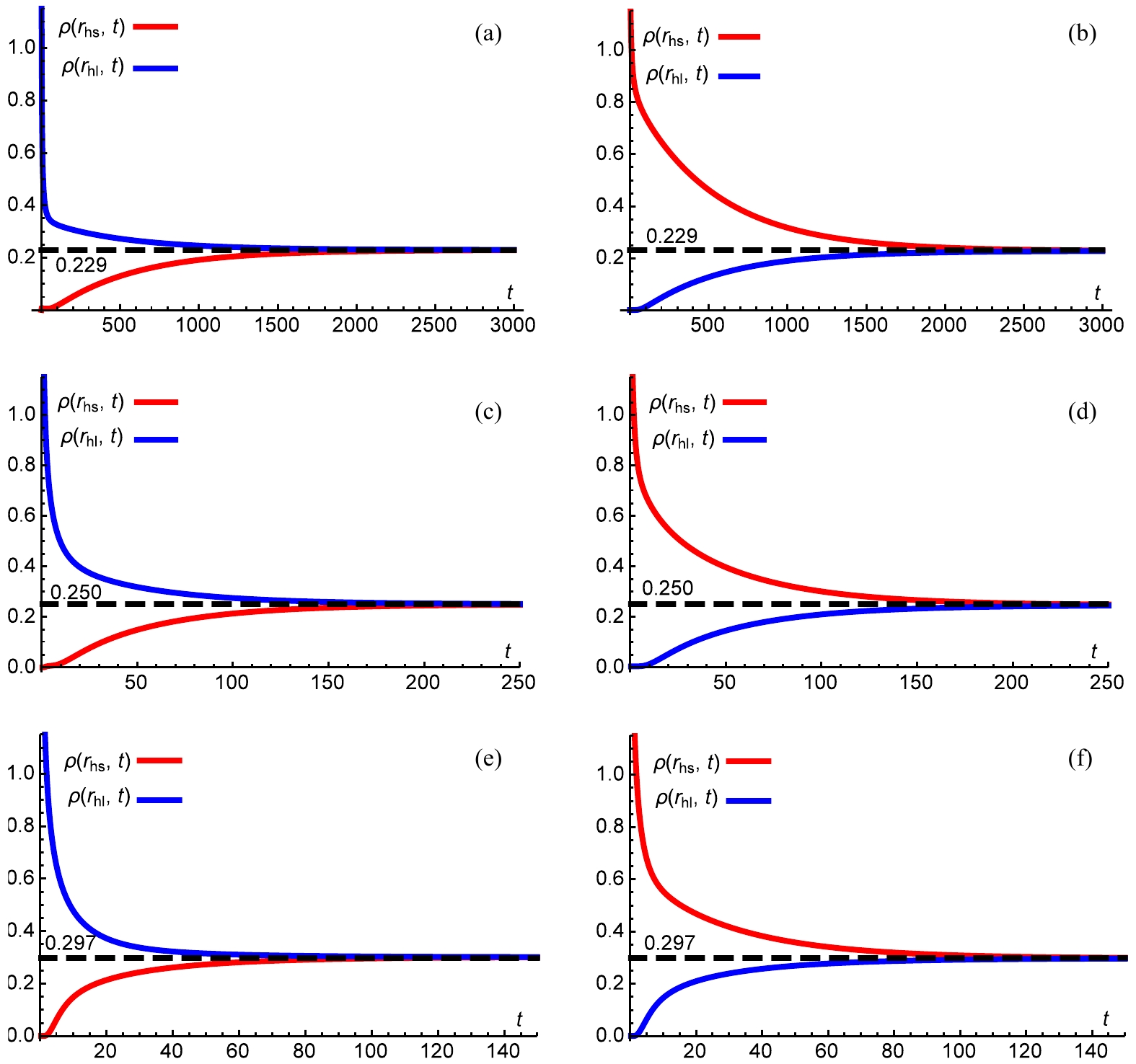
Figure 3. (color online) Time evolution of
$ \rho(r_l,t) $ and$ \rho(r_s,t) $ for charged dilaton black hole with$ b = 1,\; q = 1,\; P = 0.003 $ . (a)$ \alpha = 0.4 $ , (b)$ \alpha = 0.4 $ , (c)$ \alpha = 0.2 $ , (d)$ \alpha = 0.2 $ , (e)$ \alpha = 0 $ , and (f)$ \alpha = 0 $ . For the left three graphs, the initial condition is chosen as a Gaussian wave packet located at the large dilaton black hole state, while for the right three graphs, the initial condition is chosen as a Gaussian wave packet located at the small dilaton black hole state.$ \alpha $ 

0 0.2 0.4 $ \Delta G_{L} $ 

0.00115 0.00951 0.11993 Table 1. Height of the barrier
$ \Delta G_{\rm L} $ as a function of$ \alpha $ with$ b = 1,\; q = 1,\; P = 0.003 $ . -
To further investigate the dynamic phase transition of dilaton black holes, the first passage process was considered. This process describes how the initial black hole state approaches the intermediate transition state for the first time. To numerically investigate this process, both the reflecting boundary condition and absorbing boundary condition were imposed. Note that the absorbing boundary condition
$ \rho(r_m,t) = 0 $ [58] was imposed at the intermediate transition state with the horizon radius denoted as$ r_m $ .Through resolving the Fokker-Planck equation constrained by these two boundary conditions, the first passage process of charged dilaton black holes is displayed in Fig. 4. Similarly, the initial condition was chosen as a Gaussian wave packet located at the large dilaton black hole state for the left three graphs, while the Gaussian wave packet located at the small dilaton black hole state was chosen for the right three graphs. Regardless of the initial black hole state, the initial peaks decayed rapidly. We also compared the time evolution for different values of
$ \alpha $ . For the top, middle, and bottom rows of Fig. 4,$ \alpha $ values were chosen as 0.4, 0.2, and 0, respectively. From this, we observed that the initial peak decays more slowly with increasing$ \alpha $ , which is consistent with the results displayed in Fig. 2 and Fig. 3.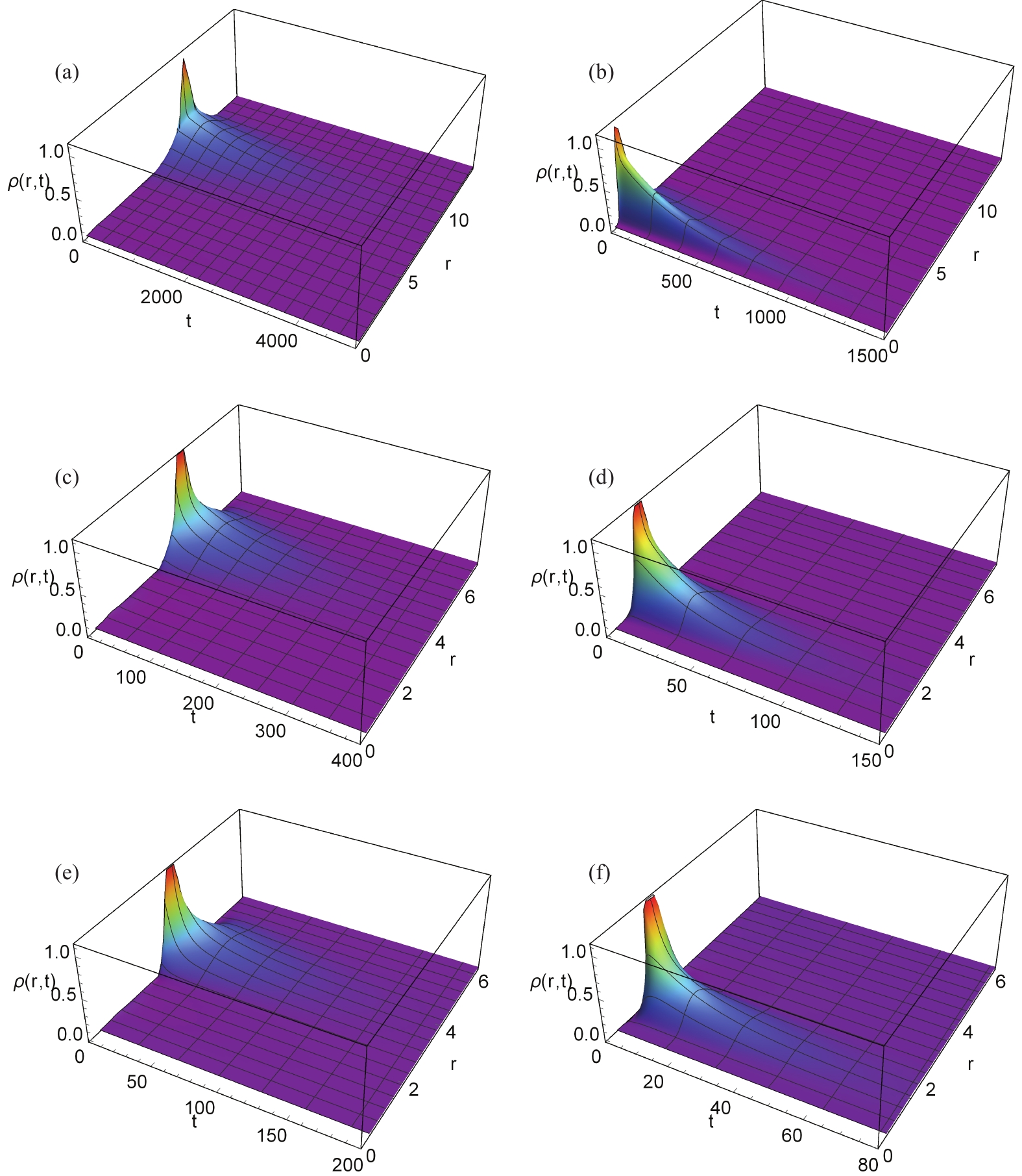
Figure 4. (color online) Time evolution of
$ \rho(r,t) $ in the first passage process of a charged dilaton black hole with$ b = 1, \;q = 1, \;P = 0.003 $ . (a)$\alpha = 0.4 $ , (b)$ \alpha = 0.4 $ , (c)$ \alpha = 0.2$ , (d)$ \alpha = 0.2 $ , (e)$ \alpha = 0$ , and (f)$ \alpha = 0 $ . For the left three graphs, the initial condition was chosen as a Gaussian wave packet located at the large dilaton black hole state, while for the right three graphs, the initial condition was chosen as a Gaussian wave packet located at the small dilaton black hole state.The time needed for the first passage process is denoted as the first passage time. Its distribution
$ F_p(t) $ can be obtained via [57]$ F_p(t) = -\frac{{\rm d}\Sigma(t)}{{\rm d}t}, $

(12) where
$ \Sigma(t) $ is the sum of the probability of the black hole system not having completed a first passage by time t.Figure 5 shows the time evolution of
$ \Sigma(t) $ . Irrespective of the initial state,$ \Sigma(t) $ decays quickly. The effect of dilaton gravity can also be observed, with$ \alpha $ values chosen as 0.4, 0.2, and 0 for the top, middle, and bottom rows of Fig. 5, respectively. With increasing$ \alpha $ , the decay of$ \Sigma(t) $ slows down.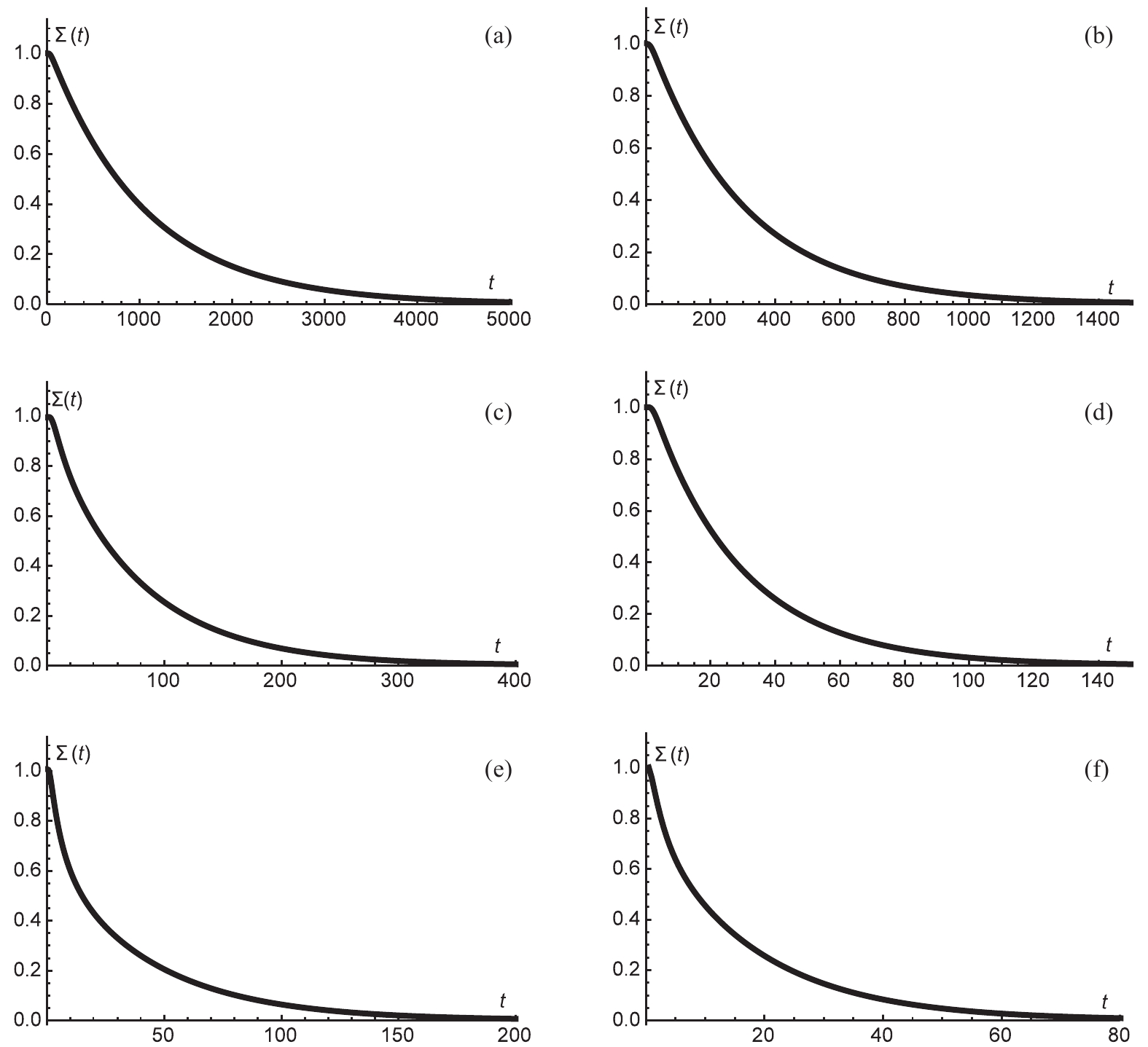
Figure 5. Time evolution of
$ \Sigma(t) $ for charged dilaton black hole with$ b = 1, \;q = 1,\; P = 0.003 $ . (a)$ \alpha = 0.4 $ , (b)$ \alpha = 0.4 $ , (c)$ \alpha = 0.2 $ , (d)$ \alpha = 0.2 $ , (e)$ \alpha = 0 $ , and (f)$ \alpha = 0 $ . For the left three graphs, the initial condition was chosen as a Gaussian wave packet located at the large dilaton black hole state, while for the right three graphs, the initial condition was chosen as a Gaussian wave packet located at the small dilaton black hole state.$ F_p(t) $ can also be derived via Eqs. (11) and (12) as [58]$ F_p(t) = -D\frac{\partial \rho(r,t)}{\partial r}\Big|_{r_m}. $

(13) This distribution of first passage time is depicted in Fig. 6. Only a single peak is present in each graph of
$ F_p(t) $ , suggesting that the first passage process takes place very quickly. Additionally, the time corresponding to the peak increases with the parameter$ \alpha $ .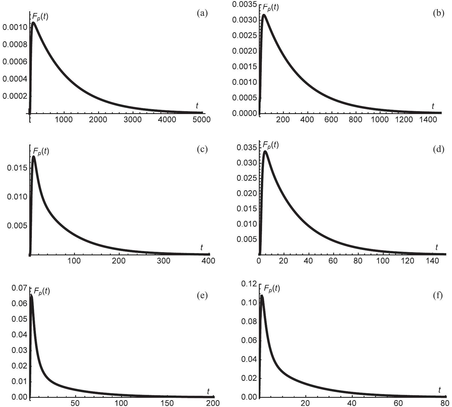
Figure 6.
$ F_p(t) $ for charged dilaton black hole with$ b = 1,\; q = 1,\; P = 0.003 $ . (a)$ \alpha = 0.4 $ , (b)$ \alpha = 0.4 $ , (c)$ \alpha = 0.2 $ , (d)$ \alpha = 0.2 $ , (e)$ \alpha = 0 $ , and (f)$ \alpha = 0 $ . For the left three graphs, the initial condition was chosen as a Gaussian wave packet located at the large dilaton black hole state, while for the right three graphs, the initial condition was chosen as a Gaussian wave packet located at the small dilaton black hole state. -
We investigated the effect of dilaton gravity on the dynamic phase transition of black holes with a focus on charged dilaton black holes. Specifically, we considered the variation of the parameter
$ \alpha $ , which describes the strength of the coupling between the electromagnetic field and the dilaton field.We introduced the Gibbs free energy landscape and calculated the corresponding
$ G_{\rm L} $ of the dilaton black hole. Based on$ G_{\rm L} $ , we numerically solved the Fokker-Planck equation. To investigate the probabilistic evolution of dilaton black holes, we first considered the reflecting boundary condition. When the initial condition is assigned to the large dilaton black hole, the initial peak of$ \rho(r,t) $ , corresponding to the radius of the large dilaton black hole, decreases with time. Concurrently, a second peak corresponding to the radius of the small dilaton black hole is observed to grow. Eventually, these peaks reach a stationary distribution where the values of$ \rho(r_{\rm l},t) $ and$ \rho(r_{\rm s},t) $ are the same. This process illustrates how the initial large dilaton black hole evolves dynamically into the small dilaton black hole. A similar but converse result was observed when the initial condition was assigned to the small dilaton black hole. The effect of dilaton gravity on the probabilistic evolution of dilaton black holes was also investigated. Firstly, the horizon radius difference between the large dilaton black hole and small dilaton black hole increased with the parameter$ \alpha $ . Secondly, with increasing$ \alpha $ , the time required to achieve a stationary distribution also increased. Note that these two observations do not depend on the initial condition. Finally, the values of$ \rho(r_{\rm l},t) $ and$ \rho(r_{\rm s},t) $ varied with the parameter$ \alpha $ (0.229 for the case of$ \alpha = 0.4 $ , 0.250 for$ \alpha = 0.2 $ , and 0.297 for$ \alpha = 0 $ ).To further investigate the dynamic phase transition of dilaton black holes, we considered the first passage process, which describes how the initial black hole state approaches the intermediate transition state for the first time. Both the reflecting boundary condition and the absorbing boundary condition were imposed in this case. Resolving the Fokker-Planck equation constrained by these two boundary conditions, we demonstrated the first passage process of charged dilaton black holes intuitively. Regardless of the initial state of the black hole, the initial peak decreased rapidly. We compared the evolution for different values of
$ \alpha $ , which revealed that the initial peak decayed more gradually with increasing$ \alpha $ . We also studied the distribution of the first passage time$ F_p(t) $ and the sum of the probability$ \Sigma(t) $ of the black hole system not having completed a first passage by time$ t $ . Irrespective of the initial state,$ \Sigma(t) $ decays very quickly. The effect of dilaton gravity was also observed. With increasing$ \alpha $ , the decay of$ \Sigma(t) $ slowed down. There was only a single peak in each graph of$ F_p(t) $ , suggesting that the first passage process takes place very quickly. Additionally, the time corresponding to the peak was found to increase with$ \alpha $ .In conclusion, the dilaton field was found to slow down the dynamic phase transition process between a large black hole and a small black hole. Furthermore, it will be interesting to investigate the effect of the dilaton field on the dynamic process of the novel phase transition described in Ref. [30].
-
The authors would like to express their sincere gratitude to the referee whose comments have helped improve the quality of this manuscript significantly.
Dynamic phase transition of charged dilaton black holes
- Received Date: 2021-05-04
- Available Online: 2021-10-15
Abstract: The dynamic phase transition of charged dilaton black holes is investigated in this paper. The Gibbs free energy landscape is introduced, and the corresponding


 DownLoad: