


 Abstract
 HTML
HTML Reference
 Related
 PDF
PDF


-
Cosmic rays are observed high energy particles coming from outer space. The energy range of cosmic rays is significantly wide, from
$ 10^6 $ to$ 10^{20} $ eV. The particles with energies higher than 1 EeV are known as ultra-high energy cosmic rays. They are believed to originate outside our galaxy [1], e.g., from an active galactic nucleus. The most likely sources for the lower energy cosmic rays are galactic supernova remnants [1-3]. The shock waves produced by the supernova explosion accelerates particles to relativistic speeds, known as shock acceleration. However, shock acceleration does not explain all the cosmic rays; alternative acceleration mechanisms have not been excluded. In the early stage of pulsar discover, it was proposed that pulsars can generate cosmic rays [4, 5]. Most charged particle acceleration mechanisms related to pulsars refer to the pulsar magnetosphere structure. In a gap region of the magnetosphere, where the plasma force-free condition could break down, particles can be accelerated by the residual electric field around pulsars [6-9]. Other acceleration mechanisms rely on plasma properties in the magnetosphere; for instance, electromagnetic energy of the plasma can be transferred into kinetic energy of particles, such as Landau damping [10] or magnetic reconnection [11-13].The pulsar magnetosphere model was proposed by Goldreich and Julian [14]. Its recent developments mainly rely on numerical simulations [15-19]. In principle, the pulsar magnetosphere model is constructed by initially inserting a magnetic dipole. Then, one obtains charged matter distribution of pulsars with plasma force-free condition. The condition can still be satisfied outside the pulsars leading to co-rotation plasma around pulsars, known as the magnetosphere. In the magnetosphere, the accelerated electric field can be entirely screened. This introduces controversies about particle acceleration from pulsars and motivates varieties of acceleration mechanisms to be proposed [6-13].
In the seminal paper [16], Spitkovsky obtained numerical solutions for a realistic pulsar magnetosphere. However, the inserted dipole in the magnetosphere model for oblique rotational pulsar is not a solution to the d'Alembert equations. In this paper, we set up a scenario for acceleration mechanism of cosmic rays in pulsars using an exact solution of the d'Alembert equations, known as the Hertzian magnetic dipole [20-22]. The electromagnetic field configuration of pulsars and the dipole radiation are presented. Particle acceleration via the electromagnetic field of a rotational magnetic dipole is studied numerically. To avoid the impacts of possible magnetosphere structure, charged particles are initially located out of the light cylinder radius, where electric field strength exceeds the magnetic field and magnetosphere may not form. The paper is organized as follows. In section II, we show that the Hertzian magnetic dipole adequately describes the electromagnetic properties of pulsars. In section III, we discuss particle acceleration in the rotational magnetic dipole field. It is shown that particles out of the light cylinder radius can be accelerated significantly. Finally, the conclusions and remarks are provided in section IV.
-
Pulsars are highly magnetized rotational celestial objects. To describe the magnetic properties of the pulsars, the magnetic monopole model [23, 24], dipole model [25, 26], or multipole model [27] have been suggested. The dipole model was widely accepted and discussed [15, 28]. In the solar system, the earth and Jupiter also have magnetic dipole fields. Unlike the earth, the pulsars generally have a strong magnetic field. In addition, due to rapid rotation of pulsars, its induced electric field is significantly strong. Pulsars are usually not a single rotational magnetic dipole in space. The strong electromagnetic field can cause electron-positron production. Moreover, the charged particles are rapidly filled with the region of the magnetosphere [6]. The co-rotation plasma in the magnetosphere increases the complexity of the electromagnetic structure of pulsars to some degree. Recent studies mostly rely on numerical methods [16-19].
The observation of pulsars depends on their electromagnetic properties. For pulsars, the most interesting feature is that the emissions are observed at a regular time interval, which can be attributed to the rotation of pulsars and the anisotropy distribution of radiation emission from pulsars. The standard picture of the pulsars is presented by acceleration gap models [6-9, 14]. The charged particles can be accelerated from a gap region of a pulsar, such as a region near magnetic poles of the pulsar in Goldreich's model [14]. In other regions, the electric field can be screened. Thus, the emission beam from the pulsars is originated from the accelerated particles that move along the curved magnetic field line, namely, the curvature radiation. The observation processes are described phenomenologically by a hollow cone model [29, 30]. It geometrically assumes that the emission beams consist of a cone from the magnetic poles of pulsars. Pulsars rotate rapidly together with magnetic poles. The emission beam can not be observed until the cone sweeps to the earth. When the magnetic poles of pulsars point to the earth, the emission beam is observed; it shows a rotational period of a pulsar.
Most of the pulsars are believed to be neutron stars. They are of about
$ M_{\odot} $ mass; their radiuses are less than 20 km. Recently, for the first time, a white dwarf star was identified as a pulsar [31]. The emission beam can be X-ray, radio, and gamma-ray [32, 33]. It can be observed by space or ground telescopes. To date, thousands of pulsars have been observed [15]. These pulsars rotate with regular periods in the range from$ 10^{-3} $ to 10 s. Especially, millisecond pulsars have the most regular rotation frequency. Pulsar timing arrays comprising millisecond pulsars are used to detect gravitational waves.The surface magnetic field of pulsars ranges from
$ 10^4 $ to$ 10^{11}\; {\rm{T}}$ [34]. No detectors are sent to a pulsar. The inferred magnetic fields of pulsars are estimated via the evolution of their rotation frequency Ω. Rotational kinetic energy loss of pulsars equals to the magnetic dipole radiation; it is known as the spin-down equation and given as$ \dot{\Omega} = - \frac{2}{3I c^3} \Omega^3 M^2 \sin^2 \theta. $

(1) The symbols will be explained later. Eq. (1) is established by assuming the simplest magnetic dipole radiation in vacuum. For the realistic pulsar magnetosphere [16], it does not significantly change the spin-down luminosity. For a large distance from a celestial object, it can be treated as a point-like object. The most simplified pulsar can be described as a point-like rotational magnetic dipole M. We further show that an exact solution of the d'Alembert equation can describe the rotational magnetic dipole of pulsars. The so-called Hertzian magnetic dipole is of the form [20-22]
$ \phi \left( t, {\boldsymbol{x}} \right) = 0, $

(2) $ {\boldsymbol{A}} \left( t, {\boldsymbol{x}} \right) = \left( {\boldsymbol{M}} + \frac{r}{c} {\dot{\boldsymbol{M}}} \right)_{\rm{ret}} \times \frac{{\boldsymbol{r}}}{r^3} , $

(3) where
$ {\dot{\boldsymbol{M}}} = {\bf{\Omega}} \times {\boldsymbol{M}}, $

(4) c is the speed of light, Ω is the rotational velocity of pulsars, and
$ {\boldsymbol{M}}_{\rm{ret}} \equiv {\boldsymbol{M}} \left( t - {r}/{c} \right) $ ; A is the retarded potential. For a quasi-static magnetic dipole$ {\dot{\boldsymbol{M}}} \equiv 0 $ , the potential reduces to the common case$ {\boldsymbol{A}} = ({\boldsymbol{M}} {\times} {\boldsymbol{r}})/{r^3} $ . By using the solution, we can calculate the electromagnetic field,$ \begin{aligned}[b] {\boldsymbol{B}} \left( t, {\boldsymbol{x}} \right) =& {\bf{\nabla}} \times {\boldsymbol{A}} = \left( - \frac{{\boldsymbol{M}}}{r^3} - \frac{1}{r^2 c} {\dot{\boldsymbol{M}}} - \frac{1}{rc^2} \ddot{{\boldsymbol{M}}} + \frac{3 {\boldsymbol{r}}}{r^5} \left( {\boldsymbol{r}} {\cdot} {\boldsymbol{M}} \right) \right.\\ &\left. + \frac{3 {\boldsymbol{r}}}{r^4} \left( {\boldsymbol{r}} {\cdot} \frac{1}{c} {\dot{\boldsymbol{M}}} \right) + \frac{{\boldsymbol{r}}}{r^3} \left( {\boldsymbol{r}} {\cdot} \frac{1}{c^2} \ddot{{\boldsymbol{M}}} \right) \right)_{\rm{ret}}, \end{aligned}$

(5) $ {\boldsymbol{E}} \left( t, {\boldsymbol{x}} \right) = - {\bf{\nabla}} \phi - \frac{1}{c}\frac{\partial {\boldsymbol{A}}}{\partial t} = - \frac{1}{c} \left( {\dot{\boldsymbol{M}}} + \frac{r}{c} \ddot{{\boldsymbol{M}}} \right)_{\rm{ret}} \times \frac{{\boldsymbol{r}}}{r^3}. $

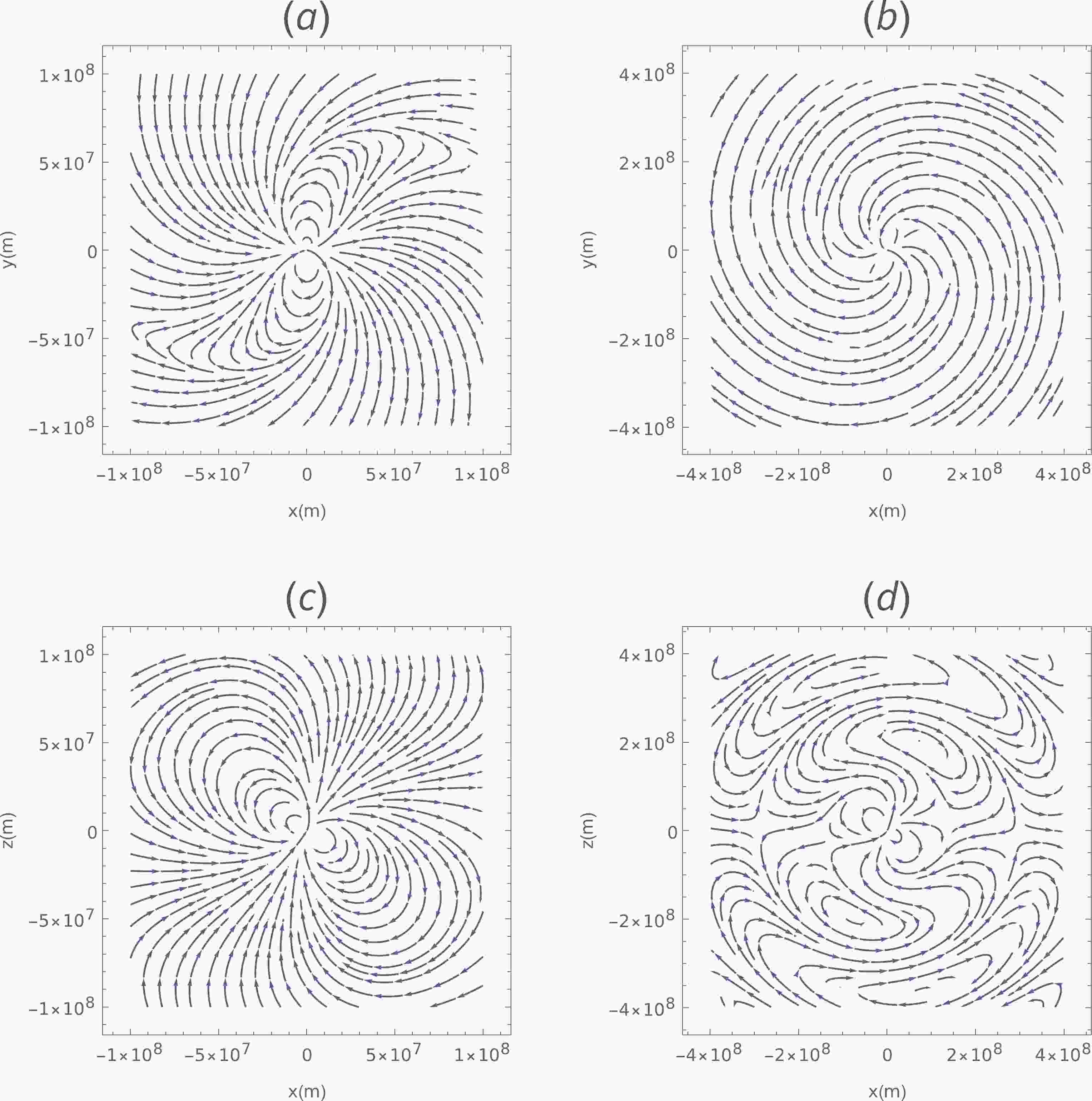
(6) Using Eq. (5) and Eq. (6), one may investigate configurations of the electromagnetic field of pulsars. Fig. 1 shows the magnetic field lines in 2 dimension. Retardation of the magnetic field is apparent at a far distance, especially where
$ r > {c}/{\Omega} $ . The 2-dimensional flow lines provide considerable insight of the magnetic field, although it is not legal as the coordinate along the projective direction is not a cyclic coordinate. Fig. 2 shows the 3-dimensional magnetic field lines. The corresponding electric fields are shown in Fig. 3. All electric field lines are circles. The retard of the electric field is indicated via the difference of the concentric axes of the cycles. One might be familiar with the magnetic field structure of the pulsars in Fig. 2(a), since the magnetic field generated by variation of magnetic dipole$ {\dot{\boldsymbol{M}}} $ is neglected in the analytical model [14, 15]. Perhaps, based on the analytical model, the magnetic field was initially set to be generated by the quasi-static magnetic dipole in numerical studies on magnetic field structure of pulsars [16, 19]. Interestingly, the analytical solution (Eq. (5)) shown in Fig. 1(a) has similarities with the numerical results [16, 19]. It may suggest that the electromagnetic field generated by the variation of the dipole$ \dot{M} $ is included in the dynamical evolution of electromagnetism. The analytical solutions in Eqs. (5) and (6) may provide a better understanding of the numerical results.
Figure 1. (color online) The 2-dimension magnetic field lines for a uniform rotational pulsar with angular speed
$ \Omega = 2\pi $ , inclination angular$ \theta = {\pi}/{6} $ and magnetic moment$ M = 10^{27}\;{\rm{Am}}^2 $ . (a) and (b) are projective magnetic field lines at x-y plane with$ z = 0 $ section. (c) and (d) are projective magnetic field lines at x-z plane with$ y = 0 $ section.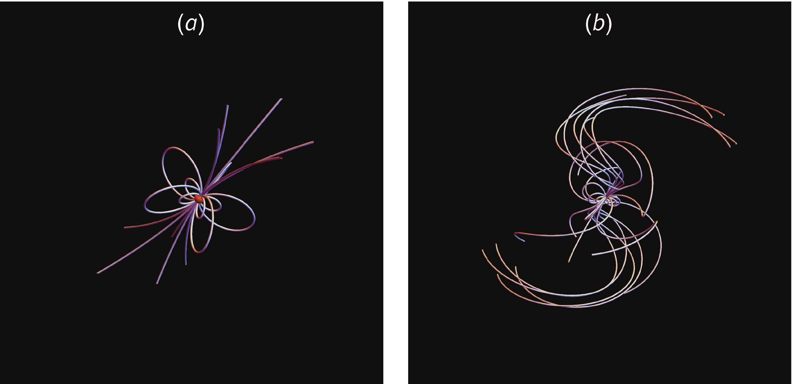
Figure 2. (color online) The 3-dimension magnetic field lines for a uniform rotation pulsar, whose angular speed
$ \Omega = 2\pi $ , inclination angular$ \theta = {\pi}/{6} $ , and magnetic moment$ M = 10^{27}\;{\rm{Am}}^2 $ . (a) is plotted in near region and (b) is plotted in far region.
Figure 3. (color online) The 3-dimension electric field lines for a uniform rotational pulsar, whose angular speed
$ \Omega = 2\pi $ , inclination angular$ \theta = {\pi}/{6} $ , and magnetic moment$ M = 10^{27}\;{\rm{Am}}^2 $ . (a) is plotted in near region and (b) is plotted in far region.One can also understand the results in Figs. 2 and 3 via analytical approximations. In the near-field region,
$ r\ll c/\Omega $ , the magnetic field and electric field reduce to$ {\boldsymbol{B}}(t,{\boldsymbol{x}}) = \frac{1}{r^3}(3\hat{{\boldsymbol{r}}} (\hat{{\boldsymbol{r}}} \cdot {\boldsymbol{M}})-{\boldsymbol{M}} )\; , $

(7) $ {\boldsymbol{E}}(t, {\boldsymbol{x}}) = \frac{1}{c r^2}(\hat{{\boldsymbol{r}}}\times ({\bf{\Omega}}\times {\boldsymbol{M}}))\; , $

(8) where
$ {\hat{\boldsymbol{r}}} \equiv {\boldsymbol{r}}/r $ . In this case, the magnetic field dominates the electromagnetic field originating from the pulsars$ E(r,{\boldsymbol{x}}) \simeq \frac{r\Omega}{c} B(r,{\boldsymbol{x}})\ll B(r,{\boldsymbol{x}})\; . $

(9) The magnitude of the electromagnetic field takes the form
$ B(t,{\boldsymbol{x}}) = \frac{M^2}{r^3}\sqrt{3\sin^2\beta+1}\; , $

(10) $ E(t,{\boldsymbol{x}}) = \frac{M \Omega}{c r^2} \sqrt{\cos^2\beta + \cos^2\alpha -2\cos\theta \cos\alpha \cos\beta}\; , $

(11) where
$ \cos\alpha \equiv \dfrac{{\boldsymbol{r}}\cdot{\bf{\Omega}}}{r \Omega} $ and$ \cos\beta \equiv \dfrac{{\boldsymbol{r}}\cdot{\boldsymbol{M}}}{r M} $ . Eq. (9) also suggests that charged particles can satisfy the force-free condition if they move at the speed of$ r\Omega $ . In the far-field region,$ r\gg c/\Omega $ , one can obtain the electromagnetic field in the form$ {\boldsymbol{B}}(t,{\boldsymbol{x}}) = \frac{1}{c^2 r}(\hat{{\boldsymbol{r}}}(\hat{{\boldsymbol{r}}}\cdot \ddot{\boldsymbol{M}})-\ddot{\boldsymbol{M}})_{\rm{ret}}\; , $

(12) $ {\boldsymbol{E}}(t, {\boldsymbol{x}}) = \frac{1}{c^2 r}(\hat{{\boldsymbol{r}}}\times \ddot{\boldsymbol{M}}_{\rm{ret}})\; , $

(13) where
$ \ddot{\boldsymbol{M}}\equiv {\dot{\bf{\Omega}}}\times{\boldsymbol{M}}+{\bf{\Omega}}\times({\bf{\Omega}}\times{\boldsymbol{M}}) $ . In this case, the magnitude of the electric field and magnetic field are comparable, namely,$ E(t,{\boldsymbol{x}}) \simeq B(t,{\boldsymbol{x}}) = \frac{M \Omega^2}{c^2 r}\sqrt{\frac{\dot{\Omega}^2}{\Omega^4}\sin^2\gamma+\sin^2\theta}+{\cal{O}}\left({\frac{c}{r\Omega}}\right)\; , $

(14) where
$ \cos\gamma\equiv \dfrac{{\boldsymbol{M}}\cdot {\dot{\bf{\Omega}}}}{M \dot{\Omega}} $ . The result in Eq. (14) is not surprising, since electromagnetic plane waves in vacuum also have the relation$ E(t,{\boldsymbol{x}}) = B(t,{\boldsymbol{x}}) $ .Pulsars rotate with dissipation because of electromagnetic radiation. It is described by the spin-down equation. The radiation reaction torque is calculated by the surface integral at spatial infinity,
$ {\boldsymbol{N}} = - \oint_S \left( {\boldsymbol{r}} \times {\boldsymbol{T}} \right) {\cdot} {{\rm{d}}} {\boldsymbol{\sigma}} = - \frac{2}{3c^3} \left( {\dot{\boldsymbol{M}}} \times \ddot{{\boldsymbol{M}}} \right)_{\rm{ret}}, $

(15) where T is the spatial part of the energy-momentum tensor,
$ T_{ij} = -({1}/(4 \pi)) \left( E_{i} E_j + B_i B_j - ({1}/{2}) \delta_{i j} (E^2 + B^2) \right) $ . Due to the integral,$ {\boldsymbol{M}}_{\rm{ret}} = {\boldsymbol{M}}(t-t_0) $ , where$ t_0 $ turns out to be a constant retard time. For simplicity, we ignore the subscript "ret" in the following. Using conservation of angular momentum of pulsars together with Eq. (4) and Eq. (15), we establish the spin-down equation,$ \begin{aligned}[b] I {\dot{\bf{\Omega}}} =& {\boldsymbol{N}} = - \frac{2}{3 c^3} ({\bf{\Omega}} \times {\boldsymbol{M}}) \times ({\dot{\bf{\Omega}}} \times {\boldsymbol{M}} + {\bf{\Omega}} \times ({\bf{\Omega}} \times {\boldsymbol{M}})) \\ =& - \frac{2}{3 c^3} ({\bf{\Omega}} ({\bf{\Omega}} \times {\boldsymbol{M}})^2 - {\boldsymbol{M}} ({\dot{\bf{\Omega}}} \times {\bf{\Omega}}) {\cdot} {\boldsymbol{M}}), \end{aligned}$

(16) where I is the inertia of momentum of pulsars. The second term can be neglected.
$ \begin{aligned}[b] 0 =& I ({\dot{\bf{\Omega}}} \times {\bf{\Omega}}) {\cdot} {\boldsymbol{M}} = \Big( \Big( - \frac{2}{3 c^3} ({\bf{\Omega}} ({\bf{\Omega}} \times {\boldsymbol{M}})^2 \\ & - {\boldsymbol{M}} ({\dot{\bf{\Omega}}} \times {\bf{\Omega}}) {\cdot} {\boldsymbol{M}}) \Big) \times {\bf{\Omega}} \Big) {\cdot} {\boldsymbol{M}} . \end{aligned} $

(17) Therefore, the vector version of the spin-down equation is of the form
$ {\dot{\bf{\Omega}}} = - \frac{2}{3Ic^3} \left( {\bf{\Omega}} \times {\boldsymbol{M}} \right)^2 {\bf{\Omega}}. $

(18) The spin-down equation indicates that pulsars rotate with a fixed inclination angle
$ \dot{\theta} = \frac{{\rm{d}}}{{\rm{d}} t} \cos^{- 1} \left( \frac{{\bf{\Omega}} {\cdot} {\boldsymbol{M}}}{\Omega M} \right) = \frac{({\boldsymbol{M}} \times {\bf{\Omega}}) {\cdot} ({\bf{\Omega}} \times {\dot{\bf{\Omega}}})}{\sin \theta M \Omega^3} = 0 . $

(19) The electromagnetic luminosity is consistent with the familiar magnetic dipole radiation
$ L = I \Omega\dot{\Omega} = - \frac{2}{3 I c^3} ({\bf{\Omega}} \times {\boldsymbol{M}})^2 {\bf{\Omega}} {\cdot} {\bf{\Omega}} = - \frac{2}{3 c^3} \Omega^4 M^2 \sin^2 \theta. $

(20) The canonical spin-down Eq. (1) can be obtained directly. It indicates that the Hertzian magnetic dipole well describes the pulsars. From the spin-down Eq. (18), one can obtain the braking index, which is the observable quantity describing rotation evolution of pulsars. In our model, the fixed inclination angle means a fixed braking index
$ n = \frac{\ddot{\Omega} \Omega}{\dot{\Omega}^2} = 3. $

(21) It differs from the results where the pulsar is considered as a perfectly conducting sphere [35], whose braking index is larger than 3 and increases with time. The spin-down equation derived from the Hertzian magnetic dipole provides consistent results with the canonical spin-down equation. Because the observations suggested that the braking indices of pulsars are greater than 3 [36-42], the Hertzian magnetic dipole model cannot tackle the problem of braking indices either.
-
The electromagnetic field of a pulsar is one of the strongest field among astronomy objects. The surface magnetic field of pulsars ranges from
$ 10^4 $ to$ 10^{11} $ T [34]; the corresponding magnetic moment ranges from$ 10^{23} $ to$ 10^{30} $ Am2. We investigate the particle acceleration in the electromagnetic field of a pulsar by using direct acceleration. Charged particles experience the Lorentz force along with their radiation damping. The dynamics of charged particles can be described by the Abraham-Lorentz-Dirac equations [43, 44],$ m \frac{{{\rm{d}}} u^{\mu}}{{{\rm{d}}} \tau} = \frac{q}{c} F^{\mu}_{\nu} u^{\nu} + g^\mu, $

(22) where
$ F^{\mu}_{\nu} $ is the electromagnetic tensor,$ F^{\mu}_{\nu} = \delta^{\mu 0} E_{\nu} + $ $ \delta_{0\nu} E^{\mu} + \epsilon_{0 \nu \lambda}^{\mu} B^{\lambda} $ ,$ g^\mu $ is the radiation reaction force,$ g^\mu = \frac{2 q^2}{3mc^4}\left(\partial_\rho F^{\mu}_{\sigma}u^\rho u^\sigma + \frac{q}{mc}F^{\mu}_{\sigma}F^{\sigma}_{\rho}u^\rho + \frac{q}{m c^3}F^{\nu}_{\sigma}F^{\sigma}_{\rho}u_\nu u^\rho u^\mu \right), $

(23) and
$ u^{\nu} $ is 4-velocity of a charged particle. There are no differences between the superscripts and subscripts of electric and magnetic fields. Here,$ E_i = E^i, B^i = B_i $ , and their 0 components are zero. From Eqs. (22) and (23), we know that$ u^\mu $ satisfies the normalization condition of 4-velocity,$ u^{\mu} u_{\nu} = - c^2 $ .In the electromagnetic field of pulsars, the electric field drives particles to high energies. Details of kinetic energies and trajectories of particles can be obtained from the solution of Eq. (22). We solve the equations numerically for protons and set protons static at a distance beyond the light cylinder radius. It may avoid the impacts of possible magnetosphere structures.
To show the acceleration quantitatively, we simulate proton acceleration numerically for different magnetic moments M with selected angular velocities of pulsars and initial positions of particles. The results are presented in Fig. 4. For selected initial positions, protons are accelerated and move away from the pulsars, whereas for initial positions that are marginally closer to the pulsars, the protons tend to fall into the pulsars. After being accelerated and thrown away, the kinetic energies of particles do not change significantly and range from 104 to 1015 eV. The accelerated energies increase with the magnetic moments. For elucidating the particle acceleration, we present the trajectories and time-evolution of kinetic energies of the photons in Fig. 5. The processes of acceleration are fast. The charged particles might be around the pulsar at first, and then run away at seconds.
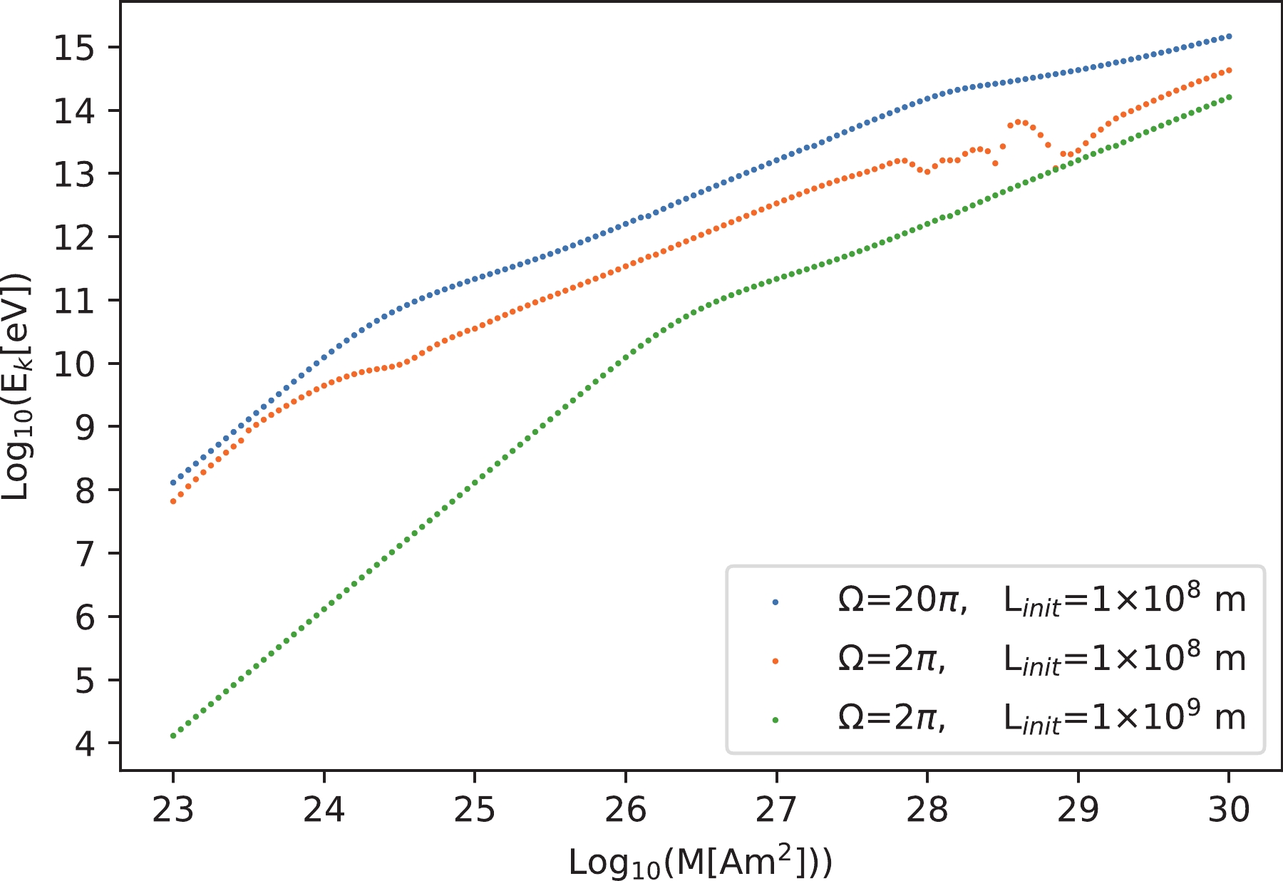
Figure 4. (color online) The kinetic energies of accelerated protons as a function of magnetic moment of pulsars. The inclination angle of pulsars
$\theta = {\pi}/{6}$ , angular speed$\Omega = 2\pi$ or$20\pi$ , and magnetic moment ranges from$10^{23}$ to$10^{30}\;{\rm{Am}}^2$ . Particles are initially static in the equatorial plane that is orthogonal to the magnetic axis with distance$L_{\rm{init}} = 10^8$ or$ 10^9\;{\rm{m}}$ from the pulsars.
Figure 5. (color online) (left) Trajectories of selected protons experience the electromagnetic field of a pulsar. (right) The kinetic energies of selected accelerated protons as a function of coordinate time t. The inclination angle of pulsars
$\theta = {\pi}/{6}$ , angular speed$\Omega = 2\pi$ , and magnetic moment$M = 10^{27}\;{\rm{Am}}^2$ . Particles are initially static in the equatorial plane that is orthogonal to the magnetic axis with distance$L_{\rm{init}} = 0 .7\times10^8\;{\rm{m}}$ (black curve),$10^8\;{\rm{m}}$ (red curve), and$2 \times 10^8\;{\rm{m}}$ (blue curve), respectively. They are all initially beyond the light cylinder.For particles initially located at different azimuth angles, the accelerated kinetic energies are also different. We simulate the proton acceleration numerically. They are initially static at a distance from pulsars and uniformly distributed at a sphere surface. For selected parameters, the distribution of accelerated kinetic energies is showed in Fig. 6(a). The ranges of the energies are no more than two orders. After being accelerated, Fig. 6(b) shows that a large number of particles are thrown away from the equatorial plane of the pulsar.

Figure 6. (color online) The kinetic energies of accelerated protons as a function of the initial azimuth angle (a) and velocity direction (b) of the protons in the celestial coordinate system using Sinusoidal projection. The pulsar is rotating around the axis-y in the celestial coordinates. The inclination angle of pulsars
$ \theta = {\pi}/{6} $ , angular speed$ \Omega = 3\pi $ , magnetic dipole$ M = 10^{27}\;{\rm{Am}}^2 $ . The protons are initially static at a distance$ 10^8 $ m away from pulsars and uniformly distributed around a sphere surface. In Fig. (a), different colors represent the kinetic energy of the accelerated protons. In Fig. (b), the grey level represents the kinetic energy.The kinetic energies of the accelerated particles originated from the rotational energy of the pulsar. Therefore, we have to estimate how many particles can be accelerated in our model. For the Crab nebula, the power of rotational energy losses is about
$ W = 10^{38} $ erg s−1 [28]. The maximum density of accelerated protons out of the light cylinder can be$ \rho_{\rm{max}} \gtrsim \left(\frac{W \times (1 {\rm{s}})}{E_k}\right) \frac{m_p}{ R_{\rm{lc}}^3} \simeq 10^{-13} \;{ {\rm{kg}}/}{\rm{m}}^{3}\; , $

(24) where we set the kinetic energy of protons
$ E_k\simeq 10^{12} $ eV, radius of the light cylinder$ R_{\rm{lc}} \simeq 10^8 {\rm{m}} $ , and$ m_p $ is the proton mass. Since the density of the interstellar medium is much less than$ \rho_{\rm{max}} $ , the accelerated protons out of the light cylinder will not have much influence on the rotation of the pulsars. -
We investigated the configurations of the electromagnetic field of pulsars by using the Hertzian magnetic dipole, an exact solution of the d'Alembert equations. We set up a scenario for the acceleration mechanism of cosmic rays in pulsars. The particles out of the light cylinder radius can be accelerated directly up to a very high energy.
In our pulsar model, the induced electric field can accelerate all the charged particles around the pulsars up to a relativistic speed. The accelerated particles, which experience the magnetic field of pulsars, can emit synchrotron radiation. The emission of the radiation can propagate through space and be finally observed by the detectors on earth [45]. It is simple enough and totally beyond the standard picture of the pulsars presented by the acceleration gap model [14, 15]. Interestingly, although a different electromagnetic field structure of the pulsar is suggested by our model, our results on the particle acceleration out of the light cylinder radius are similar to those from the numerical studies using particle-in-cell simulations [19, 46, 47] and the study based on the transitional pulsar model [14].
Here, we assumed that the increase in kinetic energy of charged particles originated from the rotational energy of a pulsar. Namely, the particles are accelerated via the electromagnetic force. The corresponding reaction force, namely, the reaction torque, will cause the spin-down of the pulsar. If this is true, as shown in Eq. (24), the rotational energy loss for accelerating the particles can be fairly neglected.
For particle acceleration, the initial states of the particles were set manually for theoretical studies. Thus, one cannot obtain the energy spectrum of the accelerated particles originating from the pulsars if the profiles of the charged particles around the pulsars and out of the light cylinder are not given.
There are two major limitations of the model. First, in the near region with respect to the finite body of pulsars, the point-like rotational magnetic dipole for pulsars will not be reasonable. Second, a possible magnetosphere structure related to our model has not been studied. The magnetosphere structure may influence particle acceleration. However, in order to avoid the structure impacts as much as possible, all the particles are chosen initially beyond the region where the possible magnetosphere might be formed. Moreover, there is still a possibility that the magnetosphere will change the electromagnetic field described by Eqs. (5) and (6). This should be further confirmed via numerical simulation using the initial conditions described by Eqs. (5) and (6), instead of the quasi-static one.
-
The authors wish to thank Dr.Zhi-Chao Zhao and Yong Zhou for useful discussions. Q.-H. Zhu is grateful to Yu-Chen Ding for useful discussions related to cosmic rays in the early stage of the work.
Particles accelerated in Hertzian magnetic dipole field of a pulsar
- Received Date: 2021-04-12
- Available Online: 2021-11-15
Abstract: Supernova remnants are supposed to be the most possible sources of cosmic rays. However, alternative sources of cosmic rays, such as an active galactic nucleus, gamma-ray bursts, and pulsars, have not be excluded. In this study, we investigate the possibility of cosmic rays being generated by pulsars. The pulsar is simply described as a rotational magnetic dipole, the so-called Hertzian magnetic dipole, an exact solution of the d'Alembert equations. In the rotational magnetic dipole field, charged particles experience an accelerated electric field with their radiation reaction. The particles, which are initially static out of the light cylinder radius, can be accelerated up to a high energy.


 DownLoad: