


 Abstract
 HTML
HTML Reference
 Related
 PDF
PDF


-
A fully microscopic proton-neutron symplectic model (PNSM) of nuclear collective motion with Sp(12,R) dynamical algebra was introduced few years ago by considering the symplectic geometry and possible collective flows in the two-component many-particle nuclear system [1]. Its more general motion group GL(6,R)
$ \subset $ Sp(12,R) introduces the wider class of allowed classical motions, including both the in-phase and out-of-phase proton-neutron collective excitations; by utilizing them, the PNSM naturally generalizes the one-component Sp(6,R) symplectic model [2, 3]. The collective states in the PNSM were initially classified by the basis states of the six-dimensional harmonic oscillator by considering the following dynamical symmetry reduction chain: Sp(12,R)$ \supset $ U(6)$ \supset $ SU$ _{p} $ (3)$ \otimes $ SU$ _{n} $ (3)$ \supset $ SU(3)$ \supset $ SO(3). Using this chain, the PNSM was applied for the simultaneous description of the microscopic structure of the lowest ground,$ \beta $ , and$ \gamma $ bands in$ ^{166} {\rm{Er}}$ [4],$ ^{152} {\rm{Sm}}$ [5],$ ^{154} {\rm{Sm}}$ [6], and$ ^{238} {\rm{U}}$ [7]. The results for the microscopic structure of negative-parity states of the lowest$ K^{\pi} = 0^{-}_{1} $ and$ K^{\pi} = 1^{-}_{1} $ bands in$ ^{152} {\rm{Sm}}$ ,$ ^{154} {\rm{Sm}}$ and$ ^{238} {\rm{U}}$ were also reported [5, 8, 9], including the low-energy$ B(E1) $ interband transition strengths between the states of the ground band and$ K^{\pi} = 0^{-}_{1} $ band [5, 9] for these three nuclei. A significant achievement of the presented approach is the simultaneous description of low-lying$ B(E2) $ and$ B(E1) $ transition strengths without introducing an effective charge.The PNSM Sp(12,R) dynamical algebra has many subalgebra chains, which can be divided into two types: the shell-model and the collective-model chains. The first type of reduction chains focuses on the many-fermion nature of the nuclear systems and relates them to the microscopic shell-model theory of nuclear structure, whereas the second type of subalgebraic chains of Sp(12,R) reveals the dynamical content of the possible collective motions in atomic nuclei. The shell-model reduction chains also define different shell-model coupling schemes in which different collective Hamiltonians can be diagonalized. In the present paper, we consider the PNSM matrix elements with respect to the following reduction chain Sp(12,R)
$ \supset $ SU(1,1)$ \otimes $ SO(6)$ \supset $ U(1)$ \otimes $ SU$ _{pn} $ (3)$ \otimes $ SO(2)$ \supset $ SO(3), which was recently shown to correspond to a microscopic version [10] of the Bohr-Mottelson [11] collective model. A characteristic property of this dynamical symmetry limit is that the collective dynamics separates into radial and orbital parts. According to this, the Hilbert space of the nucleus in the PNSM can be represented as a direct sum of many-particle shell-model subspaces labeled by the SO(6) seniority quantum number$ \upsilon $ , which carry an irreducible representation (irrep) of a direct product group SU(1,1)$ \otimes $ SO(6).The general structure SU(1,1)
$ \otimes $ SO(d) appears in the central-force problems in d-dimensional Euclidean space [12]. Then, the SO(d)-invariant Hamiltonians can be diagonalized with the SU(1,1) Lie algebra used as a spectrum generating algebra. The specific cases of$ d = 3,5 $ were widely considered in the literature. For example, the algebraic solutions of the three-dimensional central-force problems were widely studied in terms of the algebra of the direct product group SU(1,1)$ \otimes $ SO(3) (see, e.g., [13, 14]). This algebraic structure accounts for the Davidson potential, originally introduced to describe the rotation-vibrational excitations of diatomic molecules in three-dimensional space [15]. In nuclear physics, the five-dimensional Davidson potential that has an SU(1,1)$ \otimes $ SO(5) algebraic structure was used by many authors [16-19] in relation with the rotations and vibrations of atomic nuclei. Recently, the Algebraic Collective Model (ACM), also based on the SU(1,1)$ \otimes $ SO(5) algebraic structure, was formulated [20, 21] as an algebraic version of the Bohr-Mottelson [11] collective model which has the valuable property of diagonalizing [16] the$ \gamma $ -unstable Wilits-Jean-type Hamiltonians [22].The SU(1,1)
$ \otimes $ SO(5) structure was also used in the boson quasi-spin formalism [23], related to the IBM [24], treating boson particles in$ l = 2 $ orbital level (i.e., considering d bosons). Thus, this algebraic structure considers the pairing between the d bosons in IBM and diagonalizes an L = 0 pairing interaction which is an SO(5) invariant. Additionally, using the duality relationships [25] of U(1)$ \subset $ SU(1,1) and SU(d)$ \supset $ SO(d) structures, two-level paring boson Hamiltonians expressed in terms of the boson quasi-spin SU(1,1) algebra have been considered in [26].The five-dimensional Davidson potential within the framework of the (one-component) Sp(6,R) symplectic model was used to compute the detailed microscopic collective shell-model wave functions of the ground band in
$ ^{166}{\rm Er} $ in [27]. The six-dimensional Davidson potential, based on the SU(1,1)$ \otimes $ SO(6) algebraic structure, was initially introduced in Ref. [28] in the context of the phenomenological Interacting Vector Boson Model [29], which is a trivial closed-shell irrotational-flow collective submodel of the PNSM of Bohr-Mottelson type.The purpose of the present work is to develop a computational technique for the reduction chain Sp(12,R)
$ \supset $ SU(1,1)$ \otimes $ SO(6)$ \supset $ U(1)$ \otimes $ SU$ _{pn} $ (3)$ \otimes $ SO(2)$ \supset $ SO(3) of the PNSM, which will allow performing realistic shell-model calculations for determining the microscopic structure of heavy mass nuclei with various collective properties. This reduction chain provides an alternative basis for the shell-model diagonalization of an arbitrary collective Hamiltonian, which can be expressed as a polynomial in the many-particle position and momentum coordinates of the two-component proton-neutron nuclear systems, or is given in the algebraic form. The nuclear wave functions on this basis are presented as a direct product of SU(1,1) radial wave functions with the SO(6) spherical harmonics. Then, if one knows the matrix elements of the basic many-particle Jacobi position$ x_{is}(\alpha) $ and momentum$ p_{is}(\alpha) $ operators, the SU(1,1)$ \otimes $ SO(6) algebraic structure allows us to obtain the matrix elements of any function of them (lying in the enveloping algebra of the Sp(12,R) or WSp(12,R) dynamical groups; cf. Ref. [9]) in the closed analytic form. In particular, the matrix elements of the basic building blocks of the PNSM and the Sp(12,R) symplectic generators are obtained along the considered reduction chain. Using the latter, one can compute other more complicated matrix elements of different physical operators. For example, the matrix elements of the SU(3) mixing interactions that couple various shell-model configurations within and between different oscillator shells are also given. This will extend the applicability of the PNSM in describing the collective properties in various nuclei. This is illustrated by considering a simple application of this theory to the microscopic description of the rotational states of the lowest positive-parity bands in$ ^{106} {\rm{Ru}}$ and$ ^{158} {\rm{Gd}}$ . -
A certain shell-model reduction chain of the PNSM is naturally explored if the following raising and lowering operators of harmonic oscillator quanta, i.e.,
$ \begin{aligned}[b] &b^{\dagger}_{i\alpha,s} =\sqrt{\frac{m_{\alpha}\omega}{2\hbar}}\Bigg(x_{is}(\alpha) -\frac{\rm i}{m_{\alpha}\omega}p_{is}(\alpha)\Bigg), \\ &b_{i\alpha,s} = \sqrt{\frac{m_{\alpha}\omega}{2\hbar}}\Bigg(x_{is}(\alpha) +\frac{\rm i}{m_{\alpha}\omega}p_{is}(\alpha)\Bigg) \end{aligned} $

(1) are introduced. Then, a basis for the Sp(12,R) algebra is given by the all bilinear combinations of these harmonic oscillator operators [30]:
$ F_{ij}(\alpha,\beta) = \sum\limits_{s = 1}^{m}b^{\dagger}_{i\alpha,s}b^{\dagger}_{j\beta,s}, $

(2) $ G_{ij}(\alpha,\beta) = \sum\limits_{s = 1}^{m}b_{i\alpha,s}b_{j\beta,s}, $

(3) $ A_{ij}(\alpha,\beta) = \frac{1}{2}\sum\limits_{s = 1}^{m} (b^{\dagger}_{i\alpha,s}b_{j\beta,s}+b_{j\beta,s}b^{\dagger}_{i\alpha,s}), $

(4) which are O(m)-scalar operators with
$ m = A-1 $ and$ i,j = 1,2,3 $ ;$ \alpha,\beta = p,n $ . The operators (4) and (2)$ - $ (3) are related to the proton-neutron valence-shell and giant resonance degrees of freedom, respectively.We also introduce the operators [9]:
$ B^{\dagger}_{i}(\alpha) = \sum\limits_{s}b^{\dagger}_{i\alpha,s} $

(5) and
$ B_{i}(\alpha) = \big(B^{\dagger}_{i}(\alpha)\big)^{\dagger} $ , which together with the identity operator close the six-dimensional Heisenberg-Weyl algebra hw(6) =$ \{B^{\dagger}_{i}(\alpha), B_{i}(\alpha),I\} $ and provides the basic building blocks of the PNSM.We classify the shell-model nuclear states by the following reduction chain [10]:
$ \begin{aligned} \\[-8pt]&Sp(12,R) \supset SU(1,1) \otimes SO(6) \supset U(1) \otimes SU_{pn}(3) \otimes SO(2) \supset SO(3), \\ &\qquad\langle\sigma\rangle \qquad\quad \lambda_{\upsilon} \qquad\quad \upsilon \qquad\;\;\ p \qquad \ (\lambda,\mu) \qquad\;\; \nu \quad \ \ q \quad \ L \end{aligned} $ 
(6) where below the different subgroups, the quantum numbers that characterize their irreducible representations are given. We also note that the two groups SU
$ _{pn} $ (3) and SO(2) are mutually complementary within the space of fully symmetric SO(6) irreps [31]; they form a direct-product subgroup SU$ _{pn} $ (3)$ \otimes $ SO(2)$ \subset $ SO(6). Hence, the SU$ _{pn} $ (3) irrep labels$ (\lambda,\mu) $ are in one-to-one correspondence with the SO(6) and SO(2) quantum numbers$ \upsilon $ and$ \nu $ , given by the following expression [10]:$ (\upsilon )_{6} = \bigoplus\limits_{\nu = \pm\upsilon ,\pm(\upsilon-2),...,0(\pm1)}\left(\lambda = \frac{\upsilon +\nu }{2},\mu = \frac{\upsilon -\nu }{2}\right)\otimes (\nu )_{2}. $

(7) The SU(1,1) Lie algebra, related to the radial dynamics, is generated by the shell-model operators [10]:
$ S^{(\lambda_{\upsilon})}_+ = \frac{1}{2}\sum\limits_{\alpha} F^{0}(\alpha,\alpha), $

(8) $ S^{(\lambda_{\upsilon})}_- = \frac{1}{2}\sum\limits_{\alpha} G^{0}(\alpha,\alpha), $

(9) $ S^{(\lambda_{\upsilon})}_{0} = \frac{1}{2}\sum\limits_{\alpha} A^{0}(\alpha,\alpha), $

(10) with the following commutation relations
$ [S^{(\lambda_{\upsilon})}_+,S^{(\lambda_{\upsilon})}_-] = -2S^{(\lambda_{\upsilon})}_{0}, \quad [S^{(\lambda_{\upsilon})}_{0},S^{(\lambda_{\upsilon})}_{\pm}] = \pm S^{(\lambda_{\upsilon})}_{\pm}. $

(11) The operator
$ S^{(\lambda_{\upsilon})}_{0} $ itself generates the U(1) subgroup of SU(1,1).The SU(1,1) algebra has unitary representations with orthonormal basis states
$ \{|\lambda_{\upsilon}, p \rangle; p = 0, 1, 2, \ldots\} $ that are defined by the equations$ S^{(\lambda_{\upsilon})}_+ |\lambda_{\upsilon}, p \rangle = \sqrt{(2\lambda_{\upsilon}+p)(p+1)} |\lambda_{\upsilon}, p+1 \rangle, $

(12) $ S^{(\lambda_{\upsilon})}_- |\lambda_{\upsilon}, p \rangle = \sqrt{(\lambda_{\upsilon}-1+p)p} |\lambda_{\upsilon}, p-1 \rangle, $

(13) $ S^{(\lambda_{\upsilon})}_{0} |\lambda_{\upsilon}, p \rangle = \frac{1}{2}(\lambda_{\upsilon} + 2p) |\lambda_{\upsilon}, p \rangle, $

(14) for any value of
$ \lambda_{\upsilon} $ ($ \lambda_{\upsilon} > 1 $ ), which generally defines the modified oscillator SU(1,1) irreps [12]. From Eqs. (4), (10) and (14), it is evident that the operator$ 2S_{0} \equiv H_{0} $ is the shell-model harmonic oscillator Hamiltonian whose eigenvalue is given by$ (\lambda_{\upsilon}+2p) $ in units of$ \hbar\omega $ ; the U(1)$ \subset $ SU(1,1) quantum number p is related to the U(6)$ \supset $ SO(6) irrep labels E and$ \upsilon $ (cf. Eqs. (37) and (32)) via$ p = (E-\upsilon)/2 $ .The group SO(6) can be expressed through the number-preserving generators
$ A^{LM}(\alpha,\beta) $ (4) of U(6) in the standard way by taking their antisymmetric combination [10]:$ \Lambda^{LM}(\alpha,\beta) = A^{LM}(\alpha,\beta) -(-1)^{L}A^{LM}(\beta,\alpha). $

(15) The generators of different SO(6) subgroups can be obtained by considering different tensor operators with respect to SO(3) that can be constructed from (15). In this way, the generators of the SU
$ _{pn} $ (3) group are defined by the following set of operators:$ \widetilde{q}^{2M} = \sqrt{3} i[A^{2M}(p,n)-A^{2M}(n,p)], $

(16) $ Y^{1M} = \sqrt{2}[A^{1M}(p,p)+A^{1M}(n,n)], $

(17) which are rank-2 and rank-1 tensors, respectively. The single infinitesimal operator of SO(2) is proportional to the SO(3) scalar operator
$ \Lambda^{0}(\alpha,\beta) $ :$ M = \Lambda^{0}(\alpha,\beta) = {\rm i}[A^{0}(\alpha,\beta)-A^{0}(\beta,\alpha)]. $

(18) The operators given in Eqs. (16)-(18) are 9 in number, which are obtained from
$ \Lambda^{LM}(\alpha,\beta) $ when$ \alpha\neq \beta $ for L=0,2 and$ \alpha=\beta $ for L=1. The operators$ Y^{1M} (17) $ are actually a linear combination of the independent rank-1 tensors$ A^{1M}(p,p) $ and$ A^{1M}(n,n) $ , which are 6 in number. The Lie algebra of SO(6) is 15-dimensional, so the remaining 3 generators are obtained from$ \Lambda^{LM}(\alpha,\beta) $ for$ \alpha\neq \beta $ and L=1, which represent the components of rank-1 tensor$ A^{1M}(p, n) $ +$ A^{1M}(n,p) $ . Using the relations$ L^{p}_{1M} = $ $ \sqrt{2}A^{1M}(p,p) $ and$ L^{n}_{1M} = \sqrt{2}A^{1M}(n,n) $ , which define the angularmomentumoperators of the proton and neutron many-particle subsystems, respectively, the SO(6) group is thus generated by the following set of operators SO(6)$ = \{\widetilde{q}^{2M}, Y^{1M}, M, L^{p}_{1M}-L^{n}_{1M}, A^{1M}(p,n) + A^{1M}(n,p)\}$ . The operators$ L^{p}_{1M}-L^{n}_{1M} $ correspond to the infinitesimal generators of the isovector out-of-phase angular-momentum displacements of the proton subsystem with respect to the neutron one, i.e. the scissors mode excitation operators.The basis functions along the chain (6) can thus be written in the form [10]
$ \Psi_{\lambda_{\upsilon}p;\upsilon\nu qLM}(r,\Omega_{5}) = R^{\lambda_{\upsilon}}_{p}(r)Y^{\upsilon}_{\nu qLM}(\Omega_{5}), $

(19) where
$ Y^{\upsilon}_{\nu qLM}(\Omega_{5}) $ are the SO(6) Dragt's spherical harmonics [32, 33]. However, the explicit form of the latter is not required for our purposes because the calculation of the SO(6)-reduced matrix elements involving the SO(6) spherical harmonics can be carried out in a purely algebraic way. Due to the complementarity relationship [25, 31] of radial and orbital dynamics groups, SU(1,1) and SO(6), the states of seniority$ \upsilon $ of the PNSM span a unitary representation of the direct product group SU(1,1)$ \otimes $ SO(6) and satisfy the equations$ S^{(\lambda_{\upsilon})}_+ R^{\lambda_{\upsilon}}_{p}(r)Y^{\upsilon}_{\nu qLM}(\Omega_{5}) = \sqrt{(\lambda_{\upsilon}+p)(p+1)} R^{\lambda_{\upsilon}}_{p+1}(r)Y^{\upsilon}_{\nu qLM}(\Omega_{5}), $

(20) $ S^{(\lambda_{\upsilon})}_- R^{\lambda_{\upsilon}}_{p}(r)Y^{\upsilon}_{\nu qLM}(\Omega_{5}) = \sqrt{(\lambda_{\upsilon}-1+p)p} R^{\lambda_{\upsilon}}_{p-1}(r)Y^{\upsilon}_{\nu qLM}(\Omega_{5}), $

(21) $ S^{(\lambda_{\upsilon})}_{0} R^{\lambda_{\upsilon}}_{p}(r)Y^{\upsilon}_{\nu qLM}(\Omega_{5}) = \frac{1}{2}(\lambda_{\upsilon} + 2p) R^{\lambda_{\upsilon}}_{p}(r)Y^{\upsilon}_{\nu qLM}(\Omega_{5}), $

(22) where for the harmonic oscillator series
$ \lambda_{\upsilon} = \upsilon + 6/2 $ . The full many-particle Hilbert space of the nucleus thus can be represented as a direct sum$ \mathbb{H} = \bigoplus\limits_{\upsilon} \mathbb{H}^{SU(1,1)}_{\upsilon} \otimes \mathbb{H}^{SO(6)}_{\upsilon} $

(23) of Hilbert spaces labeled by a seniority quantum number
$ \upsilon $ , each carrying an irrep of the direct product group SU(1,1)$ \otimes $ SO(6). -
The Cartesian coordinates
$ \{x_{a} \equiv x_{i}(\alpha) = \sum\nolimits_{s} x_{is}(\alpha)\} $ acting in the Euclidean space$ \mathbb{R}^{6} $ can be expressed in the form$ x_{a} = r\mathcal{Q}_{a} \equiv r\mathcal{Q}_{i}(\alpha), $

(24) which is their expression in the SO(6) spherical polar coordinates. The operators
$ B^{\dagger}_{i}(\alpha) $ (5) and their conjugates$ B_{i}(\alpha) = \big(B^{\dagger}_{i}(\alpha)\big)^{\dagger} $ transform according to the U(6) fundamental irreducible representation$ [1]_{6} $ and its conjugate$ [1]^{\ast}_{6} = [1,1,1,1,1,0] \equiv [-1]_{6} $ , respectively. Under the SO(6) subgroup, both U(6) representations reduce to the irrep$ (1)_{6} $ . Then, from$ x_{i}(\alpha) = \dfrac{1}{\sqrt{2}}[B^{\dagger}_{i}(\alpha) + $ $ B_{i}(\alpha)] $ and the factorization of the position coordinates into radial and polar parts, one obtains that$ \mathcal{Q}\equiv\mathcal{Q}_{i}(\alpha) $ is the basic$ \upsilon = 1 $ SO(6) tensor. Any operator that can be represented as a polynomial in$ x_{a} $ will then have matrix elements that factor into radial and orbital parts. -
The radial matrix elements of even powers of r can be obtained utilizing only the properties of the SU(1,1) algebra. Taking into account the fact that
$ r^{2} $ is simply an element of the latter$ r^{2} = S^{(\lambda_{\upsilon})}_+ + S^{(\lambda_{\upsilon})}_- +2S^{(\lambda_{\upsilon})}_{0}, $

(25) the matrix elements of
$ r^{2} $ are immediately obtained from Eqs. (20)$ - $ (22) to be$ \begin{aligned}[b] F_{\lambda_{\upsilon}p;\lambda_{\upsilon}p'}(r^{2}) =& \langle\lambda_{\upsilon}p|r^{2}|\lambda_{\upsilon}p' \rangle \\ =& \delta_{p,p'}(\lambda_{\upsilon}+2p)/2 +\delta_{p,p-1}\sqrt{(\lambda_{\upsilon}-1+p)p} \\ & + \delta_{p,p+1}\sqrt{(\lambda_{\upsilon}+p)(p+1)} . \end{aligned} $

(26) The higher powers of
$ r^{2} $ can then be obtained by summing over intermediate states, e.g.,$ \begin{aligned}[b] F_{\lambda_{\upsilon}p;\lambda_{\upsilon}p'}(r^{4}) =& \sum\limits_{p_{c}}F_{\lambda_{\upsilon}p;\lambda_{\upsilon}p_{c}}(r^{2}) F_{\lambda_{\upsilon}p_{c};\lambda_{\upsilon}p'}(r^{2}) \\ =& \delta_{p,p'}\Big((\lambda_{\upsilon}+2p)^{2} + (\lambda_{\upsilon}+p)(p+1) + (\lambda_{\upsilon}+p-1)p\Big) \\ &+\delta_{p,p+1}\Big((2\lambda_{\upsilon}+4p+2)\sqrt{(\lambda_{\upsilon}+p)(p+1)}\Big) \\ &+\delta_{p,p-1}\Big((2\lambda_{\upsilon}+4p-2)\sqrt{(\lambda_{\upsilon}+p-1)p}\Big) \\ &+\delta_{p,p+2}\sqrt{(\lambda_{\upsilon}+p+1)(\lambda_{\upsilon}+p)(p+2)(p+1)} \\ &+\delta_{p,p-2}\sqrt{(\lambda_{\upsilon}+p-2)(\lambda_{\upsilon}+p-1)p(p-1)}. \end{aligned} $

(27) The matrix elements of
$ 1/r^{2} $ ,$rd/{\rm d}r$ ,${\rm d}^{2}/{\rm d}r^{2}$ , r,$ 1/r $ ,${\rm d}/{\rm d}r$ are given in Ref. [12]. These radial matrix elements are sufficient for deriving the matrix elements of any rotationally invariant polynomial in the many-particle collective position and momentum observables$\{x_{i}(\alpha) = $ $ \sum\nolimits_{s}x_{is}(\alpha), p_{i}(\alpha) = \sum\nolimits_{s}p_{is}(\alpha)\}$ of the PNSM. -
The SO(6)-reduced matrix elements of an arbitrary tensor
$ T^{\upsilon_{2}}_{\nu_{2}q_{2}L_{2}M_{2}} $ are defined by the generalized Wigner-Eckart theorem$\begin{aligned}[b]& \langle \upsilon_{3}\nu_{3}q_{3}L_{3} ||T^{\upsilon_{2}}_{\nu_{2}q_{2}L_{2}M_{2}} || \upsilon_{1}\nu_{1}q_{1}L_{1} \rangle \\=& \Big\langle {}^{\upsilon_{1}}_{\nu_{1}q_{1}L_{1}} \quad {}^{\upsilon_{2}}_{\nu_{2}q_{2}L_{2}}\Big| {}^{\upsilon_{3}}_{\nu_{3}q_{3}L_{3}} \Big\rangle \langle \upsilon_{3}||| T^{\upsilon_{2}}_{\nu_{2}q_{2}L_{2}M_{2}} ||| \upsilon_{1} \rangle,\end{aligned}$

(28) where
$ \Big\langle {}^{\upsilon_{1}}_{\nu_{1}q_{1}L_{1}} \quad {}^{\upsilon_{2}}_{\nu_{2}q_{2}L_{2}}\Big| {}^{\upsilon_{3}}_{\nu_{3}q_{3}L_{3}} \Big\rangle $ are the SO(6) Clebsch-Gordan coefficients. The latter, according to the Racah's lemma [34], can be factorized in terms of the isoscalar factors that appear in each step of the reduction chain (6). Taking the correspondence$ (\lambda,\mu) \leftrightarrow (\upsilon,\nu) $ given by Eq. (7), the SO(6) Clebsch-Gordan coefficients can be written in a more convenient way as$ \begin{aligned}[b] &\Big\langle {}^{\quad \upsilon_{1}}_{\nu_{1}q_{1}L_{1}} \quad {}^{\quad \upsilon_{2}}_{\nu_{2}q_{2}L_{2}}\Big| {}^{\quad \upsilon_{3}}_{\nu_{3}q_{3}L_{3}} \Big\rangle = \Big\langle {}^{\quad \upsilon_{1}}_{(\lambda_{1},\mu_{1})} \quad {}^{\quad \upsilon_{2}}_{(\lambda_{2},\mu_{2})}\Big| {}^{\quad \upsilon_{3}}_{(\lambda_{3},\mu_{3})} \Big\rangle \\ &\times \langle (\lambda_{1},\mu_{1})q_{1}L_{1}; (\lambda_{2},\mu_{2})q_{2}L_{2}|| (\lambda_{3},\mu_{3})q_{3}L_{3} \rangle , \end{aligned} $

(29) where
$ \Big\langle {}^{\quad \upsilon_{1}}_{(\lambda_{1},\mu_{1})} \quad {}^{\quad \upsilon_{2}}_{(\lambda_{2},\mu_{2})}\Big| {}^{\quad \upsilon_{3}}_{(\lambda_{3},\mu_{3})} \Big\rangle $ and$ \langle (\lambda_{1},\mu_{1})q_{1}L_{1}; (\lambda_{2},\mu_{2})q_{2}L_{2}|| $ $ (\lambda_{3},\mu_{3})q_{3}L_{3} \rangle $ are the SO(6)$ \supset $ SU(3) and SU(3)$ \supset $ SO(3) isoscalar factors, respectively. Computer codes [35, 36] exist for the calculation of the latter. From another side, by using the isomorphism SO(6)$ \approx $ SU(4) and the fact that the SO(6) tensors$ T^{(\upsilon)} $ correspond to the SU(4) tensors of the type$ T^{[\upsilon,\upsilon,0,0]} $ , the calculation of the SO(6)$ \supset $ SU(3) isoscalar factors is equivalent to the calculation of the SU(4)$ \supset $ SU(3) isoscalar factors, for which a computer code is also available [37] (Actually, the code given in [37] calculates the full SU(4)$ \supset $ SU(3)$ \otimes $ U(1)$ \supset $ SU(2)$ \otimes $ U(1)$ \supset $ U(1) Clebsch-Gordan coefficients. The structure of the code, however, allows easily to adapt the latter for the calculation of the SU(4)$ \supset $ SU(3) isoscalar factors by using the factorization property of the SU(4) Clebsch-Gordan coefficients and modifying the line 143). Therefore, matrix elements of any operators of interest can be calculated from their SO(6)-reduced matrix elements.The SO(6)-reduced matrix elements of the basic SO(6) tensor
$ \mathcal{Q} $ are given by [12]$ \langle \upsilon' | \mathcal{Q} | \upsilon \rangle = \sqrt{\frac{\upsilon+1}{2\upsilon+6}}\delta_{\upsilon',\upsilon+1} +\sqrt{\frac{\upsilon+3}{2\upsilon+2}}\delta_{\upsilon',\upsilon-1} . $

(30) The SO(6)-reduced matrix elements of other, more complicated tensors can be calculated utilizing these elementary matrix elements. For example, the SO(6)-reduced matrix elements
$ [\mathcal{Q}\times \mathcal{Q}]^{\upsilon = 2} $ , which are relevant to the mass quadrupole tensor operators$ Q_{ij}(\alpha,\beta) \rightarrow T^{\upsilon = 2}_{\nu q2m} = $ $ r^{2}Y^{\upsilon = 2}_{\nu q2m} \equiv r^{2}[\mathcal{Q}\times \mathcal{Q}]^{\upsilon = 2}_{\nu q2m} $ , are given by the standard recoupling technique:$ \langle \upsilon'|[\mathcal{Q}\times \mathcal{Q}]^{\upsilon = 2}_{\nu q2m}|\upsilon \rangle = \sum\limits_{c} U(\upsilon; 1; \upsilon'; 1||\upsilon_{c}; 2) \langle \upsilon'|\mathcal{Q}|\upsilon_{c} \rangle \langle \upsilon_{c}| \mathcal{Q}|\upsilon \rangle . $

(31) The SO(6) recoupling coefficients
$ U(\upsilon; 1; \upsilon'; 1||\upsilon_{c}; 2) $ are equivalent to the two-rowed SU(4) Racah coefficients$ U\Big([\upsilon,\upsilon]_{4}; [1,1]_{4}; [\upsilon',\upsilon']_{4}; [1,1]_{4}||[\upsilon_{c},\upsilon_{c}]; [2,2]_{4}\Big) $ . The two-rowed or two-column U(d) Racah recoupling coefficients, as well as other U(d) invariant quantities, are equivalent to those of the U(2) group, as shown, for example, by Li and Paldus in Ref. [38]. For convenience, we present some of the relevant PNSM SO(6)$ \approx $ SU(4) recoupling coefficients in Table 1.$ U(\upsilon;1;\upsilon+2;1||\upsilon+1;2) = 1 $ 

$ U(\upsilon;1;\upsilon;1||\upsilon+1;2) = -(-1)^{\upsilon}\left[\dfrac{\upsilon(\upsilon+2)}{2(2+\upsilon(\upsilon+3))}\right]^{1/2} $ 

$ U(\upsilon;1;\upsilon;1||\upsilon-1;2) = -(-1)^{\upsilon}\left[\dfrac{\upsilon(\upsilon+2)}{2\upsilon(\upsilon+1)}\right]^{1/2} $ 

$ U(\upsilon;2;\upsilon+4;2||\upsilon+2;4) = 1 $ 

$ U(\upsilon;2;\upsilon;2||\upsilon;4) = \left[\dfrac{2(\upsilon-1)(\upsilon+3)}{3\upsilon(\upsilon+2)}\right]^{1/2} $ 

$ U(\upsilon;2;\upsilon+2;2||\upsilon;2) = \left[\dfrac{\upsilon(\upsilon+1)}{2(2+3\upsilon(\upsilon+3))}\right]^{1/2} $ 

$ U(\upsilon;2;\upsilon+2;2||\upsilon+2;2) = -\left[\dfrac{(\upsilon+3)(\upsilon+4)}{2(\upsilon^{2}+5\upsilon+6)}\right]^{1/2} $ 

$ U(\upsilon;2;\upsilon;2||\upsilon+2;4) = \left[\dfrac{(\upsilon+3)\upsilon(\upsilon-1)}{6(\upsilon^{3}+6\upsilon^{2}+11\upsilon+6)}\right]^{1/2} $ 

$ U(\upsilon;2;\upsilon;2||\upsilon+2;2) = \left[\dfrac{(\upsilon+3)\upsilon}{2(\upsilon^{2}+3\upsilon+2)}\right]^{1/2} $ 

$ U(\upsilon;2;\upsilon;2||\upsilon+2;0) = (-1)^{\upsilon}\left[\dfrac{\upsilon+3}{3(\upsilon+1)}\right]^{1/2} $ 

$ U(\upsilon;2;\upsilon;2||\upsilon-2;4) = \left[\dfrac{(\upsilon-1)(\upsilon^{2}+5\upsilon+6)}{6\upsilon(\upsilon^{2}-1)}\right]^{1/2} $ 

$ U(\upsilon;2;\upsilon;2||\upsilon-2;2) = -\left[\dfrac{(\upsilon-1)(\upsilon+2)}{2\upsilon(\upsilon+1)}\right]^{1/2} $ 

$ U(\upsilon;2;\upsilon;2||\upsilon-2;0) = \left[\dfrac{\upsilon-1}{3(\upsilon+1)}\right]^{1/2} $ 

$ U(\upsilon;2;\upsilon;2||\upsilon;4) = \left[\dfrac{2(\upsilon-1)(\upsilon+3)}{3\upsilon(\upsilon+2)}\right]^{1/2} $ 

$ U(\upsilon;2;\upsilon-2;2||\upsilon-2;2) = (-1)^{-\upsilon}\left[\dfrac{\upsilon-2}{2\upsilon}\right]^{1/2} $ 

Table 1. Some SO(6) Racah recoupling coefficients.
In practice, for the calculation of the matrix elements of various algebraic interactions, it turns out to be more convenient to use the SO(6)-reduced matrix elements of the symplectic generators, which in turn are obtained from the basic creation
$ B^{\dagger}_{i}(\alpha) $ and annihilation$ B_{i}(\alpha) $ operators, respectively. The SO(6)-reduced matrix elements of these operators can be obtained by considering the equivalent chain$ \begin{aligned} &U(6) \supset SO(6), \\ &\ \ E \qquad\quad \upsilon \end{aligned} $

(32) whose branching rules for the case of fully symmetric irreps are given by [39]
$ [E]_{6} = \bigoplus\limits_{\upsilon = E,E-2,...,0(1)}(\upsilon ,0,0)_{6} = \bigoplus\limits_{i = 0}^{\langle\frac{E}{2}\rangle}(E-2i)_{6}. $

(33) The SO(6)-reduced matrix elements are therefore obtained by applying the Wigner-Eckart theorem with respect to this chain
$ \begin{align} &\langle E'\upsilon' |||B^{\dagger}_{i}(\alpha)|||E\upsilon \rangle = \langle E'|||B^{\dagger}_{i}(\alpha)|||E \rangle \Big\langle {}^{[E]}_{\ \upsilon} \quad {}^{[1]}_{\ 1}\Big| {}^{[E']}_{\ \upsilon'} \Big\rangle . \end{align} $

(34) Using the elementary (one-particle) U(d)
$ \supset $ SO(d) isoscalar factors, given in Ref. [40], one readily obtains for$ d = 6 $ :$ \langle E+1,\upsilon+1 |||B^{\dagger}_{i}(\alpha)|||E\upsilon \rangle = \sqrt{\frac{(\upsilon+1)(E+\upsilon+6)}{(2\upsilon+6)}}, $

(35) $ \langle E+1,\upsilon-1 |||B^{\dagger}_{i}(\alpha)|||E\upsilon \rangle = \sqrt{\frac{(E-\upsilon+2)(\upsilon+3)}{(2\upsilon+2)}}. $

(36) However, this result is valid only for the scalar
$ \langle \sigma \rangle = 0 $ irreducible representation of Sp(12,R), which corresponds to the doubly closed-shell nuclei; hence, it is not physically interesting. For non-scalar irreps$ \langle \sigma \rangle \neq 0 $ , the ket vectors$ | E\upsilon\widetilde{\eta} \rangle $ need to be replaced by the U(6)-coupled basis states$ |\sigma n \rho E\upsilon \widetilde{\eta} \rangle = [P^{(n)}(F) \times |\sigma \rangle]^{\rho E\upsilon}_{\widetilde{\eta}} $

(37) along the chain
$ \begin{align} &Sp(12,R) \ \supset \ U(6) \supset \ SO(6), \\ &\quad\quad \ \sigma \quad \ n\rho \quad \ E \qquad\quad \upsilon \end{align} $

(38) where
$ \widetilde{\eta} $ labels the basis of an SO(6) irrep$ \upsilon $ , classified further by the other subgroups along the chain (6). The basic creation$ B^{\dagger}_{i}(\alpha) $ and annihilation$ B_{i}(\alpha) $ operators couple the even and odd irreps of Sp(12,R) and belong to the larger collective algebra wsp(12,R) = [hw(6)]sp(12,R) [9], which is the semidirect sum of Heisenberg-Weyl algebra hw(6) =$ \{B^{\dagger}_{i}(\alpha), B_{i}(\alpha),I\} $ and symplectic algebra sp(12,R). Then, in order to calculate the matrix elements of$ B^{\dagger}_{i}(\alpha) $ and$ B_{i}(\alpha) $ , one must consider the representation theory of the$ wsp(12,R) $ which basis states can be represented as$ |\langle\langle\sigma\rangle\rangle l\langle \omega \rangle n \rho E\upsilon \widetilde{\eta} \rangle = \Big[P^{(n)}(F) \times \Big[Q^{(l)}\big(B^{\dagger}_{i}(\alpha)\big) \times |\sigma \rangle\Big]^{(\omega)}\Big]^{\rho E\upsilon}_{\widetilde{\eta}} $

(39) that are classified according to the reduction chain
$ \begin{align} &wsp(12,R) \quad \supset \quad sp(12,R) \quad \supset \quad u(6) \supset so(6) \ . \\ &\quad\langle\langle \sigma \rangle\rangle \quad\quad\;\; l \quad\quad\quad \langle \omega \rangle \quad\quad n\rho \quad\;\; E \quad\quad \ \upsilon \end{align} $

(40) For more details, we refer the reader to Ref. [9]. For the present purposes, it is sufficient to restrict the construction of the basis states to the form
$ |\sigma n\rho E\upsilon \widetilde{\eta} \rangle = \Big[Q^{(n)}\big(B^{\dagger}_{i}(\alpha)\big) \times |\sigma \rangle\Big]^{\rho E\upsilon}_{\widetilde{\eta}} . $

(41) Then, using a standard recoupling technique, the SO(6)-reduced matrix elements of the raising generators
$ B^{\dagger}_{i}(\alpha) $ of$ wsp(12,R) $ along the basis (41) can be written as$ \begin{aligned}[b] &\langle \sigma' n' \rho' E'\upsilon' |||| \ B^{\dagger}_{i}(\alpha) \ |||| \sigma n \rho E\upsilon \rangle \\ =& \langle \sigma n' \rho' E'\upsilon'|||B^{\dagger}_{i}(\alpha)|||\sigma n \rho E\upsilon \rangle \Big\langle {}^{[E]}_{\ \upsilon} \quad {}^{[1]}_{\ 1}\Big| {}^{[E']}_{\ \upsilon'} \Big\rangle \\ =& U\Big([\sigma]_{6};[n]_{6};[E']_{6};[1]_{6}\Big|\Big|[E]_{6};[n']_{6}\Big) \\ &\times\langle n' |||| \ B^{\dagger}_{i}(\alpha) \ |||| n \rangle \Big\langle {}^{[E]}_{\ \upsilon} \quad {}^{[1]}_{\ 1}\Big| {}^{[E']}_{\ \upsilon'} \Big\rangle, \end{aligned} $

(42) where the corresponding U(6) Racah coefficient is equal to 1. Using the latter, we obtain the following expressions for the SO(6)-reduced matrix elements of the creation operators
$ B^{\dagger}_{i}(\alpha) $ :$ \begin{aligned}[b] &\langle \sigma'n+1,\rho',E+1,\upsilon+1 |||B^{\dagger}_{i}(\alpha)|||\sigma n\rho E\upsilon \rangle \\ =& \sqrt{\frac{(n+1)(\sigma+n+\upsilon+6)(\upsilon+1)} {(\sigma+n+1)(2\upsilon+6)}} \ , \end{aligned} $

(43) $ \begin{aligned}[b] \\ &\langle \sigma'n+1,\rho',E+1,\upsilon-1|||B^{\dagger}_{i}(\alpha)|||\sigma n\rho E\upsilon \rangle \\ =& \sqrt{\frac{(n+1)(\sigma+n-\upsilon+2)(\upsilon+3)} {(\sigma+n+1)(2\upsilon+2)}}. \end{aligned} $

(44) where we have also used the relation
$ E = \sigma +n $ . We also observe that the quantum number n is related to the p quantum number via$ n = 2p $ ; there exists a correspondence between the harmonic oscillator basis states$ |n \rangle $ and the SU(1,1) basis$ |\lambda_{\upsilon}, p \rangle $ . To observe this, one can relabel the basis states$ |n \rangle $ of the harmonic oscillator by the SU(1,1) quantum numbers$ \{|\lambda_{\upsilon}, p \rangle; p = 0, 1, 2, \ldots\} $ . Then, one readily obtains the following correspondence$ |n \rangle = |\lambda_{\upsilon} = \frac{6}{2}, p = \frac{n}{2} \rangle, $

(45) for even n, and
$ |n \rangle = |\lambda_{\upsilon} = \frac{8}{2}, p = \frac{n-1}{2} \rangle, $

(46) for odd n values, respectively. Conversely, taking
$ |\lambda_{\upsilon}, p \rangle = |n \rangle $ with$ n = \lambda_{\upsilon} + 2p -6/2 $ and using Eqs. (2)$ - $ (4) and (8)$ - $ (10), one obtains for$ n = 0, 1, 2, \ldots $ the standard oscillator expressions$ S^{(\lambda_{\upsilon})}_+ |n \rangle = \frac{1}{2}\sqrt{(n+1)(n+2)} |n+2 \rangle, $

(47) $ S^{(\lambda_{\upsilon})}_- |n \rangle = \frac{1}{2}\sqrt{n(n-1)} |n-2 \rangle, $

(48) $ S^{(\lambda_{\upsilon})}_{0} |n \rangle = \frac{1}{2}\bigg(n + \frac{6}{2}\bigg) |n \rangle, $

(49) which are special cases (
$ \lambda_{\upsilon} = 6/2 $ and$ \lambda_{\upsilon} = 8/2 $ ) of the general expressions (12)$ - $ (14).The corresponding SO(6)-reduced matrix elements of the annihilation operators are obtained by the relation
$ \begin{aligned}[b] \langle \sigma'n'\rho'E'\upsilon'|||B_{i}(\alpha)|||\sigma n\rho E\upsilon \rangle \end{aligned} $

$ \begin{aligned}[b] = \sqrt{\frac{{\rm dim}(\upsilon)}{{\rm dim}(\upsilon')}} \langle \sigma n\rho E\upsilon|||B^{\dagger}_{i}(\alpha)|||\sigma'n'\rho'E'\upsilon' \rangle, \end{aligned} $

(50) where
${\rm dim}(\upsilon) = (\upsilon+3)(\upsilon+2)^{2}(\upsilon+1)/12$ is the dimension of the SO(6) irrep$ \upsilon $ . The result is$ \begin{aligned}[b] &\langle \sigma'n-1,\rho',E-1,\upsilon-1 |||B_{i}(\alpha)|||\sigma n\rho E\upsilon \rangle \\ =& \sqrt{\frac{n(\sigma+n+\upsilon+4)(\upsilon+2)(\upsilon+3)} {(\sigma+n)(\upsilon+1)(2\upsilon+4)}} \ , \end{aligned} $

(51) $ \begin{aligned}[b] \\ &\langle \sigma'n-1,\rho',E-1,\upsilon+1 |||B_{i}(\alpha)|||\sigma n\rho E\upsilon \rangle \\ =& \sqrt{\frac{n(\sigma+n-\upsilon)(\upsilon+1)(\upsilon+2)} {(\sigma+n)(\upsilon+3)(2\upsilon+4)}}. \end{aligned} $

(52) Using a standard recoupling technique, with the help of Eqs. (43)
$ - $ (52) and the values of the SO(6) Racah coefficients given in Table 1, one readily obtains the SO(6)-reduced matrix elements of the symplectic generators (2), (3), and (4):$ \begin{aligned}[b] \langle \sigma n+2,\rho',E+2,\upsilon+2 |||F_{ij}(\alpha,\beta)|||\sigma n\rho E\upsilon \rangle = \Bigg[\frac{(n+1)(n+2)(\sigma+n+\upsilon+6)(\sigma+n+\upsilon+8)} {(\sigma+n+1)(\sigma+n+2)} \frac{(\upsilon+1)(\upsilon+2)}{(2\upsilon+6)(2\upsilon+8)}\Bigg]^{1/2}, \end{aligned} $ 
(53) $ \langle \sigma n-2,\rho',E-2,\upsilon-2 |||G_{ij}(\alpha,\beta)|||\sigma n\rho E\upsilon \rangle = \Bigg[\frac{n(n-1)(\sigma+n+\upsilon+2)(\sigma+n+\upsilon+4)} {(\sigma+n)(\sigma+n-1)} \frac{(\upsilon+2)^{2}(\upsilon+3)}{\upsilon(2\upsilon+2)(2\upsilon+4)}\Bigg]^{1/2} , $

(54) $ \begin{aligned}[b] \langle \sigma n\rho E\upsilon+2 |||A_{ij}(\alpha,\beta)|||\sigma n\rho E\upsilon \rangle =& \frac{1}{2}\Bigg[ \frac{n(\upsilon+2)}{(\sigma+n)} \sqrt{\frac{(\sigma+n+\upsilon+6)(\sigma+n-\upsilon)(\upsilon+1)} {(\upsilon+3)(2\upsilon+4)(2\upsilon+8)}} \\ & +\frac{(n+1)}{(\sigma+n+1)(2\upsilon+6)} \sqrt{\frac{(\sigma+n+\upsilon+6)(\sigma+n-\upsilon)(\upsilon+1)(\upsilon+2)(\upsilon+3)} {(\upsilon+4)}} \Bigg] ,\end{aligned} $

(55) $ \begin{aligned}[b] \langle \sigma n\rho E\upsilon-2 |||A_{ij}(\alpha,\beta)|||\sigma n\rho E\upsilon \rangle =& \frac{1}{2}\Bigg[ \frac{n(\upsilon+2)}{(\sigma+n)} \sqrt{\frac{(\sigma+n+\upsilon+4)(\sigma+n-\upsilon+2)(\upsilon+3)} {(\upsilon+1)2\upsilon(2\upsilon+4)}} \\ & +\frac{(n+1)}{(\sigma+n+1)(2\upsilon+2)} \sqrt{\frac{(\sigma+n-\upsilon+2)(\sigma+n+\upsilon+4)(\upsilon+1)(\upsilon+2)(\upsilon+3)}{\upsilon}} \Bigg], \end{aligned} $

(56) $ \begin{aligned}[b] \langle \sigma n\rho E\upsilon|||A_{ij}(\alpha,\beta)|||\sigma n\rho E\upsilon \rangle = &-\frac{1}{2}\Bigg[\frac{n(\sigma+n+\upsilon+4)(\upsilon+2)} {(\sigma+n)(2\upsilon+4)(\upsilon+1)}\sqrt{\frac{\upsilon(\upsilon+3)}{2}} +\frac{n(\sigma+n-\upsilon)(\upsilon+2)}{(\sigma+n)(2\upsilon+4)} \sqrt{\frac{\upsilon(\upsilon+1)(\upsilon+4)}{2(2+\upsilon(\upsilon+3))(\upsilon+3)}} ,\end{aligned} $

$ \begin{aligned}[b]\quad\quad\quad\quad\quad\quad+\frac{(n+1)(\sigma+n-\upsilon+2)}{(\sigma+n+1)(2\upsilon+2)}\sqrt{\frac{\upsilon(\upsilon+3)}{2}} +\frac{(n+1)(\sigma+n+\upsilon+6)}{(\sigma+n+1)(2\upsilon+6)} \sqrt{\frac{\upsilon(\upsilon+1)(\upsilon+3)(\upsilon+4)}{2(2+\upsilon(\upsilon+3))}} \Bigg]. \end{aligned} $

(57) The coherent state theory of symplectic algebras [41-46] implies that the matrix elements of the raising and lowering symplectic operators (i.e., Eqs. (53) and (54)) are required to be multiplied by the K-matrix. However, in the limit of large representations
$ \langle \sigma \rangle $ of Sp(12,R) or in the multiplicity free case ($ \rho = \rho' = 1 $ ), which are the cases of practical importance, the K-matrix reduces to simple normalization coefficients (a diagonal K-matrix):$\sqrt{\Delta\Omega(\sigma n'E';nE)} = \sqrt{\Omega(\sigma n'E')-\Omega(\sigma nE)}, $

where
$ \Omega(\sigma nE) = \frac{1}{4}\sum\nolimits_{a = 1}^{6}[2E^{2}_{a}-n^{2}_{a}+ 14(E_{a}-n_{a})-2a(2E_{a}-n_{a})] \;[43]. $

Therefore, the final expressions for all matrix elements in which the raising and lowering symplectic generators F's and G's enter must be multiplied by the proper normalization factors.
From the matrix elements of the symplectic generators, one can obtain the SO(6)-reduced matrix elements of different algebraic interactions. For example, we present the results for the SO(6)-reduced matrix elements of the
$ \begin{aligned}[b]&A^{2}(\alpha,\beta)\cdot F^{2}(\alpha,\beta) \simeq [A^{2}(\alpha,\beta)\times F^{2}(\alpha,\beta)]^{\upsilon = 2}_{\nu = \pm2q = 1l = 0m = 0}\\& F^{2}(\alpha,\beta)\cdot F^{2}(\alpha,\beta) \simeq [F^{2}(\alpha,\beta)\times F^{2}(\alpha,\beta)]^{4}_{\pm4100} ~{\rm and} \\&G^{2}(\alpha,\beta)\cdot F^{2}(\alpha,\beta) \simeq [G^{2}(\alpha,\beta)\times F^{2}(\alpha,\beta)]^{4}_{\pm4100}\end{aligned} $

tensor operators:
$ \begin{aligned}[b] &\langle \sigma n+2,\rho',E+2,\upsilon+2 |||A^{2}(\alpha,\beta)\cdot F^{2}(\alpha,\beta)|||\sigma n\rho E\upsilon \rangle \\ =& \sqrt{\frac{5(n+1)(n+2)(\sigma+n+\upsilon+6)(\sigma+n+\upsilon+8)(\upsilon+1)(\upsilon+2)(\upsilon+3)(\upsilon+4)} {(\sigma+n+1)(\sigma+n+2)2(\upsilon^{2}+5\upsilon+6)(2\upsilon+6)(2\upsilon+8)}}\\ &\times\Bigg(\frac{(n+2)(\sigma+n+\upsilon+8)(\upsilon+4)} {(\sigma+n+2)(2\upsilon+8)(\upsilon+3)}\sqrt{\frac{(\upsilon+2)(\upsilon+5)}{2}} +\frac{(n+2)(\sigma+n-\upsilon)(\upsilon+4)}{(\sigma+n+2)(2\upsilon+8)} \sqrt{\frac{(\upsilon+2)(\upsilon+3)(\upsilon+6)} {2(2+(\upsilon+2)(\upsilon+5))(\upsilon+5)}} \\ &+\frac{(n+3)(\sigma+n-\upsilon+2)}{(\sigma+n+3)(2\upsilon+6)}\sqrt{\frac{(\upsilon+2)(\upsilon+5)}{2}} +\frac{(n+3)(\sigma+n+\upsilon+10)}{(\sigma+n+3)(2\upsilon+10)}\sqrt{\frac{(\upsilon+2)(\upsilon+3)(\upsilon+5)(\upsilon+6)} {2(2+(\upsilon+2)(\upsilon+5))}} \Bigg), \end{aligned} $ 
(58) $ \begin{aligned}[b] &\langle \sigma n+4,\rho',E+4,\upsilon+4 |||F^{2}(\alpha,\beta)\cdot F^{2}(\alpha,\beta)|||\sigma n\rho E\upsilon \rangle \\ =& \sqrt{\frac{5(n+1)(n+2)(n+3)(n+4)(\sigma+n+\upsilon+6)(\sigma+n+\upsilon+8)(\sigma+n+\upsilon+10)(\sigma+n+\upsilon+12)} {(\sigma+n+1)(\sigma+n+2)(\sigma+n+3)(\sigma+n+4)(2\upsilon+6)(2\upsilon+8)(2\upsilon+10)(2\upsilon+12)}}\\ &\times\sqrt{(\upsilon+1)(\upsilon+2)(\upsilon+3)(\upsilon+4)}, \end{aligned} $

(59) $ \begin{aligned}[b]& \langle \sigma n\rho E\upsilon|||G^{2}(\alpha,\beta)\cdot F^{2}(\alpha,\beta)|||\sigma n\rho E\upsilon \rangle \\ =& \frac{(n+1)(n+2)(\sigma+n+\upsilon+6)(\sigma+n+\upsilon+8)(\upsilon+4)} {(\sigma+n+1)(\sigma+n+2)(2\upsilon+6)(2\upsilon+8)} \sqrt{\frac{5(\upsilon-1)\upsilon(\upsilon+1)(\upsilon+3)(\upsilon+5)}{6(\upsilon^{3}+6\upsilon^{2}+11\upsilon+6)}}\\ &+\frac{(n+1)(n+2)(\sigma+n-\upsilon+2)(\sigma+n-\upsilon+4)} {(\sigma+n+1)(\sigma+n+2)(2\upsilon)(2\upsilon+2)} \sqrt{\frac{5(\upsilon-1)\upsilon(\upsilon+2)(\upsilon+3)(\upsilon^{2}+5\upsilon+6)}{6(\upsilon+1)}} . \end{aligned} $

(60) -
The full SO(3)-reduced matrix elements of physical observables of interest are obtained by multiplying the SO(6)-reduced matrix elements with the proper SO(6)
$ \supset $ SU(3) and SU(3)$ \supset $ SO(3) isoscalar factors. For example, for the SO(3)-reduced matrix elements of the raising symplectic generators we have$ \begin{aligned}[b] &\langle \sigma n+2,\rho',E+2,\upsilon+2,\nu+2,q'L'||F^{2m}(\alpha,\beta) ||\sigma n\rho E\upsilon\nu qL\rangle \\ =& \langle \sigma n+2,\rho',E+2,\upsilon+2 |||F^{2m}(\alpha,\beta)|||\sigma n\rho E\upsilon \rangle \\ &\times \Big\langle {}^{\ \ \upsilon}_{(\lambda,\mu)} \quad {}^{\ \ 2}_{(2,0)}\Big| {}^{\ \ \upsilon+2}_{(\lambda+2,\mu)} \Big\rangle \\ &\times \langle (\lambda,\mu)qL; (2,0)2|| (\lambda+2,\mu)q'L' \rangle, \end{aligned} $

(61) where the SO(6)-reduced matrix elements of
$ F^{2m}(\alpha,\beta) $ are given by Eq. (53). Similarly, one can obtain the matrix elements of other physical operators of interest. -
In practical calculation, another realization of the SO(6) algebra becomes more convenient. It is obtained using the transformation
$ \begin{aligned}[b] &a^{\dagger}_{j} = \frac{1}{\sqrt{2}}\Big(-{\rm i}B^{\dagger}_{j}(p)+B^{\dagger}_{j}(n)\Big), \\ &b^{\dagger}_{j} = \frac{1}{\sqrt{2}}\Big({\rm i}B^{\dagger}_{j}(p)+B^{\dagger}_{j}(n)\Big) \end{aligned} $

(62) and their conjugate counterparts
$ \begin{aligned}[b] &a_{j} = \frac{1}{\sqrt{2}}\Big({\rm i}B_{j}(p)+B_{j}(n)\Big), \\ &b_{j} = \frac{1}{\sqrt{2}}\Big(-{\rm i}B_{j}(p)+B_{j}(n)\Big). \end{aligned} $

(63) Then, one obtains an alternative realization of SO(6) [32, 33, 47, 48]:
$ \widetilde{q}^{2M} = \sqrt{3}[A^{2M}(a,a)-A^{2M}(b,b)],$

(64) $ Y^{1M} = \sqrt{2}[A^{1M}(a,a)+A^{1M}(b,b)], $

(65) $M = a^{\dagger}\cdot a - b^{\dagger}\cdot b = N_{a}-N_{b}, $

(66) In this realization, the creation operators
$ a^{\dagger}_{j} $ and$ b^{\dagger}_{j} $ carry the SU(3) irreps$ (1,0) $ and$ (0,1) $ , respectively. We recall that both$ B^{\dagger}_{j}(p) $ and$ B^{\dagger}_{j}(n) $ were transformed as two independent$ (1,0) $ SU(3) tensor operators. Correspondingly, the symplectic operators$ F^{2m}(a,a) $ ,$ F^{2m}(b,b) $ , and$ F^{2m}(a,b) $ transform as$ (2,0) $ ,$ (0,2) $ , and$ (1,1) $ SU(3) tensors, whereas$ A^{lm}(a,b) $ and$ A^{lm}(b,a) $ $ - $ as$ (2,0) $ and$ (0,2) $ SU(3) tensors, respectively. Then the construction of the basis (shown in Table 1 of Ref. [10]) along the chain (6) becomes straightforward. For instance:$ |E = 2, \upsilon = 2,\nu = 2,qLM \rangle \simeq F^{LM}(a,a)|0 \rangle $ ,$|E = 2, \upsilon = 2, \nu = 0, $ $ qLM \rangle \simeq F^{LM}(a,b)|0 \rangle$ ,$|E = 2,\upsilon = 2,\nu = -2, qLM \rangle \simeq $ $ F^{LM}(b,b)|0 \rangle$ , where$ |0 \rangle = |E = 0,\upsilon = 0,\nu = 0,q = 1, L = 0, $ $ M = 0 \rangle $ .The starting point of the present application is the following dynamical symmetry Hamiltonian [10]:
$ \begin{aligned}[b] H = & \ 2S^{(\lambda)}_{0} + A\Lambda^{2} + BC_{2}[SU_{pn}(3)] \\ &+ aC_{2}[SO(3)] + b(C_{2}[SO(3)])^{2}, \end{aligned} $

(67) in which the first term
$ 2S^{(\lambda)}_{0} $ , as mentioned before, represents the harmonic oscillator mean field that defines the shell structure. The eigenvalues of this Hamiltonian are the energies$ \begin{aligned}[b] E(n,\upsilon,\lambda,\mu,L) =& n \hbar\omega +A\upsilon(\upsilon+4)\\& +\frac{2}{3} B(\lambda^{2}+\mu^{2}+\lambda\mu+3\lambda+3\mu) \\ &+ aL(L+1) + b[L(L+1)]^{2}. \end{aligned} $

(68) To illustrate the present theory, we apply it to two nuclei with various collective properties, namely
$ ^{106} {\rm{Ru}}$ and$ ^{158} {\rm{Gd}}$ with the characteristic ratios$ E_{4^{+}_{1}}/E_{2^{+}_{1}} \simeq 2.65 $ and$ 3.26 $ [49], respectively. These two isotopes were chosen as examples of nuclei with different collective structures. The purpose of the present work is not to provide a detailed and accurate description of their low-lying collective spectra that are observed experimentally; instead, we aim to illustrate the application of the developed computational technique. They are chosen as nuclei having different collective properties and not specifically as possible candidates for SO(6) symmetry (the case of$ ^{106} {\rm{Ru}}$ , whose energy ratio is close to the$ \gamma $ -unstable Wilets-Jean [22] model value 2.50). As demonstrated in Ref. [10], the present version of the PNSM represents a microscopic shell-model counterpart of the Bohr-Mottelson [11] collective model, having three classical submodel limits$ - $ the$ \gamma $ -unstable Wilets-Jean model [22], the rigid-rotor model of Ui [50], and the harmonic vibrator model. Therefore, it was suggested that these three limiting types of nuclear collective behavior can be described simultaneously within the framework of the present shell-model coupling scheme of the PNSM. However, this is beyond the scope of the present paper. Detailed application of the present approach to each type of nuclear structure behavior, corresponding to a certain submodel of the BM [11] model, will be separately provided in future publications.Because in heavy mass regions, the spin-orbit interaction is strong, we use the pseudo-SU(3) scheme [51-53] to determine the relevant irreducible representations of Sp(12,R). To obtain the leading SU(3) irrep for these nuclei, i.e. the one which is maximally deformed and has maximal value of the SU(3) second-order Casimir operator, at the observed quadrupole deformation, one first fills the pseudo-oscillator Nilsson levels of the valence shells with protons and neutrons pairwise, from bottom up in energy. For instance, in the case of
$ ^{106} {\rm{Ru}}$ , we have 8 valence normal-parity neutrons in the pseudo-$ fp $ shell, which produce the$ (10,4) $ irreducible representation for the neutron subsystem. Using the Nilsson model ideas [54, 55], however, the appropriate prolate-deformed SU(3) irrep would be$ (18,0) $ that is obtained from the$ (10,4) $ one. For the proton subsystem, the valence protons completely fill the pseudo-$ ds $ shell; consequently, they produce the scalar irrep$ (0,0) $ of SU(3). Computer codes are available [56, 57] for determining the corresponding Pauli allowed SU(3) irreducible representations in a given major shell for a given number of valence nucleons. For the highest-weight SU(3) states considered here, one can also manually obtain the relevant leading irreps. In the second step, one needs to couple the proton and neutron SU(3) subirreps to obtain the relevant SU$ _{pn} $ (3) irreducible representation of the combined proton-neutron nuclear system. For$ ^{106} {\rm{Ru}}$ , this is trivially done because$ (18,0) \otimes (0,0) \rightarrow (18,0) $ . The relevant Sp(12,R) irreducible representation is fixed by the requirement that the lowest-weight U(6) irrep$\sigma = $ $ [\sigma_{1},\ldots,\sigma_{6}]_{6}$ of the symplectic bandhead should contain the SU(3) leading irrep$ (18,0) $ . Thus, the Nilsson model ideas [54, 55] and shell-model considerations based on the pseudo-SU(3) scheme for$ ^{106} {\rm{Ru}}$ provide the irreducible representation$\langle \sigma \rangle = \langle 33+\dfrac{105}{2}, 15+\dfrac{105}{2}, 15+\dfrac{105}{2}, $ $ 15+ \dfrac{105}{2}, 15+ \dfrac{105}{2}, 15+\dfrac{105}{2} \rangle$ of Sp(12,R), which corresponds to the lowest-weight U(6) irreducible representation$ \sigma = [33,15,15,15,15,15]_{6} \equiv [18]_{6} $ . The latter, according to Eqs. (7) and (33), contains the lowest-energy SU(3) irrep$ (18,0) $ of the ground state (when there is no$ SU(3) $ mixing) that is embedded in the SO(6) irreducible representation$ \upsilon_{0} = 18 $ . The set of SU$ _{pn} $ (3) irreps within the SO(6) irrep$ \upsilon_{0} = 18 $ is given by$ (18,0), (17,1), (16,2) $ ,$ \ldots,(10,8),(9,9),(8,10) $ ,$ \ldots, (2,16), $ $ (1,17),(0,18) $ . Similarly, for$ ^{158} {\rm{Gd}}$ , we obtain [10] the irreducible representation$\langle \sigma \rangle = \langle 63+\dfrac{157}{2}, 27+\dfrac{157}{2}, 27+\dfrac{157}{2}, 27+\dfrac{157}{2}, 27+\dfrac{157}{2}, 27+ $ $ \dfrac{157}{2} \rangle$ of Sp(12,R), which corresponds to the lowest-weight U(6) irreducible representation$ \sigma = [63,27,27, $ $ 27,27,27]_{6} \equiv [36]_{6} $ . Likewise, the shell model considerations for$ ^{158} {\rm{Gd}}$ give the lowest-energy SU(3) irrep$ (36,0) $ , which according to Eqs. (7) and (33), is contained in the SO(6) irreducible representation$ \upsilon_{0} = 36 $ . The full set of SU$ _{pn} $ (3) multiplets that is contained in the SO(6) irrep$ \upsilon_{0} = 36 $ , according to Eq. (7), is as follows: (36,0), (35,1), (34,2),$ \dots, $ (19,17), (18,18), (17,19),$ \ldots,$ (2,34), (1,35), (0,36). Thus, in the pure SU(1,1)$ \otimes $ SO(6) dynamical symmetry limit of the PNSM, the first excited$ \beta $ and$ \gamma $ bands in$ ^{158} {\rm{Gd}}$ belong to the SU$ _{pn} $ (3) irrep$ (34,2) $ . Similarly, the$ \gamma $ band in$ ^{106} {\rm{Ru}}$ belongs to the SU$ _{pn} $ (3) irrep$ (16,2) $ .Using Eq. (68), we compare the excitation energies of the ground and
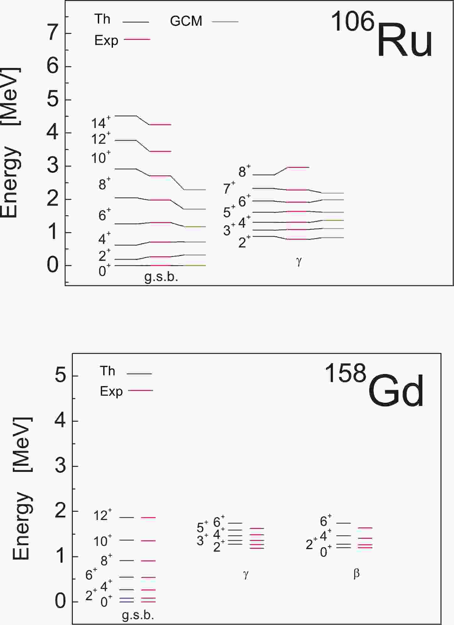
$ \gamma $ bands in$ ^{106} {\rm{Ru}}$ and those of the ground,$ \beta $ , and$ \gamma $ bands in$ ^{158} {\rm{Gd}}$ , with the experiment shown in Fig. 1. The adopted values of the model parameters in MeV are$ A = 0 $ ,$ B = -0.0324 $ ,$ a = 0.032 $ , and$ b = -0.00005 $ for$ ^{106} {\rm{Ru}}$ and$ A = 0 $ ,$ B = -0.026 $ ,$ a = 0.0134 $ , and$b = $ $ -0.0000093$ for$ ^{158} {\rm{Gd}}$ . For comparison, in the case of$ ^{106} {\rm{Ru}}$ , the results of the general collective model (GCM) with a collective potential including terms up to sixth order (with 8 free parameters) are given as well [58]. This figure shows a good agreement with the experimental data for the excitation energies of the bands under consideration for the two nuclei.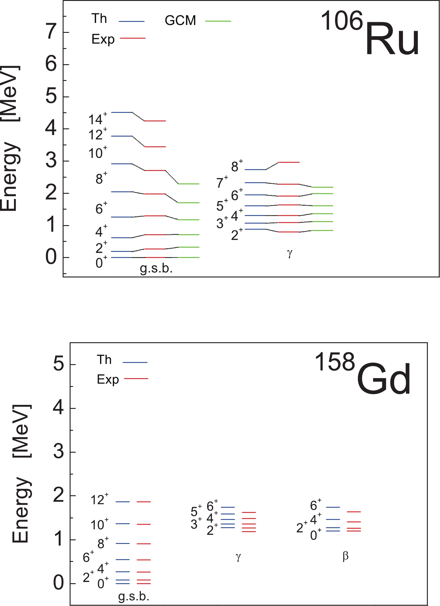
Figure 1. (color online) Comparison of the excitation energies of the ground and
$ \gamma $ bands in$ ^{106} {\rm{Ru}}$ and ground,$ \beta $ , and$ \gamma $ bands in$ ^{158} {\rm{Gd}}$ via experiments according to Eq. (68). For comparison, in the case of$ ^{106} {\rm{Ru}}$ , the results of the general collective model (GCM) with a collective potential including terms up to the sixth order are given as well [58]. -
The transition probabilities are given, by definition, by the SO(3)-reduced matrix elements of the corresponding transition operator. Here we restrict ourselves to the
$ B(E2) $ transition strengths between the states of the ground band only. We use$ T^{E2} = (eZ/(A-1)) \widetilde{q}^{2m} $ as the$ E2 $ transition operator, where$ \widetilde{q}^{2m} $ is given by Eq. (64). Because$ \widetilde{q}^{2m} $ is a generator of the SU$ _{pn} $ (3) group, we obtain the well-known result for the$ B(E2) $ transition probabilities$ \begin{aligned}[b] B(E2; L_{i} \rightarrow L_{f}) =& \frac{2L_{f}+1}{2L_{i}+1} \big|\langle f|| T^{E2} || i \rangle \big|^{2} = \frac{2L_{f}+1}{2L_{i}+1}\bigg(\frac{eZ}{A-1}\bigg)^{2}\Bigg(k\sqrt{3}\langle (\lambda,\mu)qL_{i}; (1,1)2|| (\lambda,\mu)q'L_{f} \rangle \\ &\times\sqrt{2\langle C_{2}[SU_{pn}(3)]\rangle}\Bigg)^{2}, \end{aligned} $ 
(69) where
$ \langle C_{2}[SU_{pn}(3)]\rangle = \frac{2}{3}(\lambda^{2}+\mu^{2}+\lambda\mu+3\lambda+3\mu) $ is the eigenvalue of the SU$ _{pn} $ (3) second-order Casimir operator. Additionally, because the relevant irreps in the PNSM for heavy nuclei are determined by using the pseudo-SU(3) scheme [51-53], a constant factor k enters the expression, which relates the real quadrupole operator with its pseudo-SU(3) counterpart, i.e.,$\widetilde{q}^{2m} = k\widetilde{q}^{2m}_{\rm pseudo}$ . For rare-earth and Ru regions,$ k \approx 1.20 $ and$ k \approx 1.25 $ , respectively. In present calculations, no effective charge is used (i.e.,$ e = 1 $ ).Using Eq. (69), in Fig. 2, we compare the calculated intraband
$ B(E2) $ transition probabilities between the states of the ground band in$ ^{158} {\rm{Gd}}$ with experiment [49] (dashed green line). We observe that theoretical values overestimate the experimental data. For$ ^{106} {\rm{Ru}}$ , the experimental value is known only for the transition$ B(E2;2^{+}_{1} \rightarrow 0^{+}_{1}) = 66 $ W.u. [49]. The theoretical value we obtained in the pure SU$ _{pn} $ (3) dynamical symmetry limit is 95.76 W.u. The results obtained for the$ B(E2) $ transition probabilities in the two nuclei suggest that in order to reduce the theoretical values, a horizontal mixing of different SU(3) multiplets within the corresponding SO(6) irreducible representation$ \upsilon_{0} $ is required.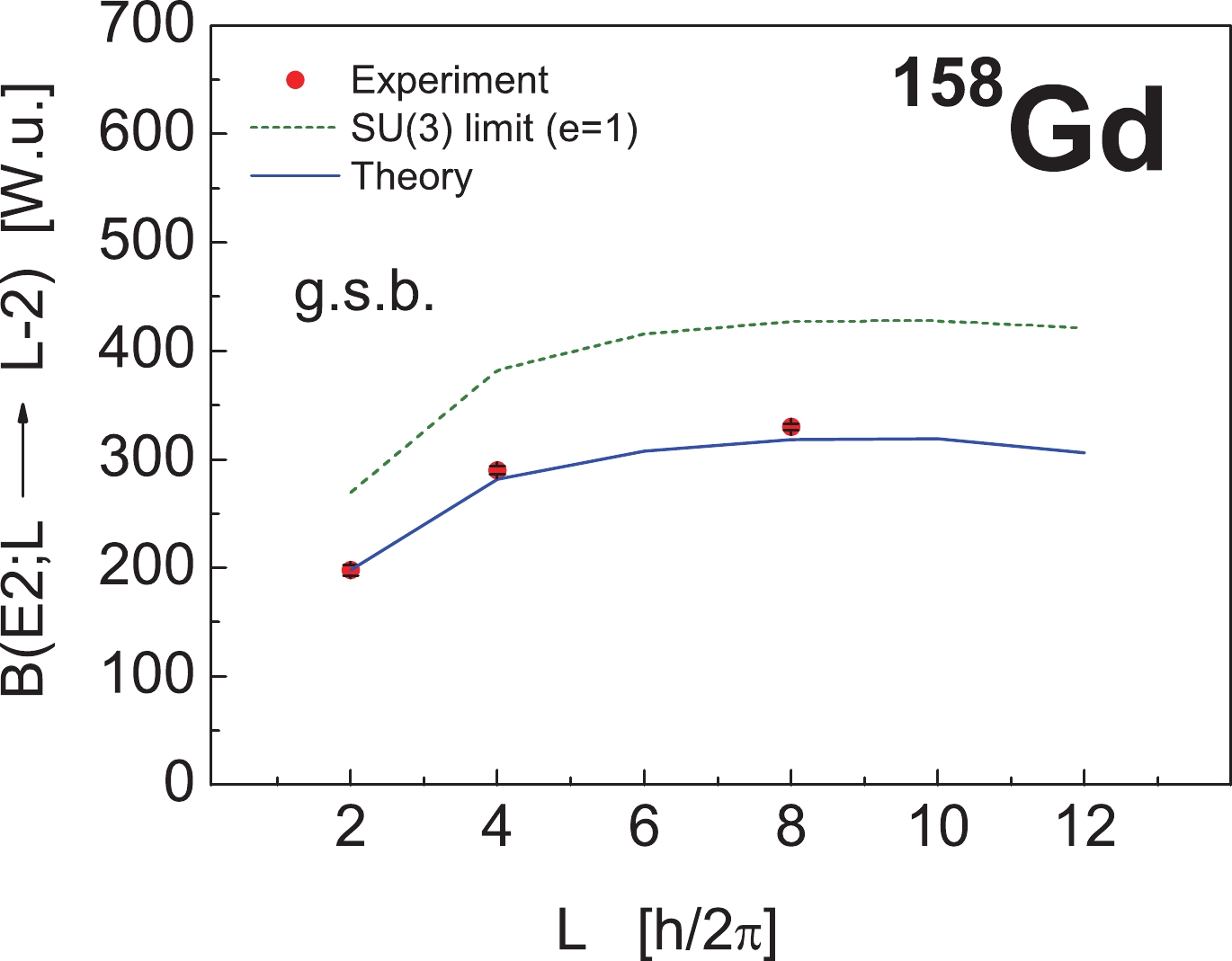
Figure 2. (color online) Calculated intraband
$ B(E2) $ values in Weisskopf units between the states of the ground band in$ ^{158} {\rm{Gd}}$ obtained in the pure SU(3) limit (dashed green line) and mixed representation calculations (continuous blue curve). No effective charge is used. -
To obtain better agreement with the experiment on
$ B(E2) $ transition probabilities, we use the following simple Hamiltonian$H_{\rm mix} = h\Big(G^{2}(a,a) \cdot F^{2}(b,b) + G^{2}(b,b) \cdot F^{2}(a,a)\Big) $

(70) that mixes different SU(3) multiplets within the maximal seniority SO(6) representation
$ \upsilon_{0} $ contained in the corresponding symplectic bandhead. Then, for example, the SO(3)-reduced matrix elements of the tensor$ G^{2}(a,a) \cdot $ $ F^{2}(b,b) = \dfrac{2\sqrt{5}}{3}[G^{2}(a,a)\times F^{2}(b,b)]^{4}_{-4100} $ are given by$ \begin{aligned}[b] &\langle \sigma \rho En\upsilon\nu'q'L||G^{2}(a,a) \cdot F^{2}(b,b)||\sigma n\rho E\upsilon\nu qL\rangle \\ =& \langle \sigma n\rho E\upsilon |||[G^{2}(a,a)\times F^{2}(b,b)]^{4}_{-4100}|||\sigma n\rho E\upsilon \rangle \\ &\times\frac{2\sqrt{5}}{3} \Big\langle {}^{\ \ \upsilon}_{(\lambda,\mu)} \quad {}^{\ \ 4}_{(0,4)}\Big| {}^{\qquad \upsilon}_{(\lambda-2,\mu+2)} \Big\rangle \\ &\times \langle (\lambda,\mu)qL; (0,4)0|| (\lambda-2,\mu+2)q'L \rangle, \end{aligned} $

(71) where the entering SO(6)-reduced matrix elements are given by Eq. (60). The SO(3)-reduced matrix elements of the tensor operator
$ G^{2}(b,b) \cdot F^{2}(a,a) = \dfrac{2\sqrt{5}}{3}[G^{2}(b,b)\times $ $ F^{2}(a,a)]^{4}_{4100} $ are similarly expressed. We recall that the corresponding SO(6)$ \approx $ SU(4)$ \supset $ SU(3) and SU(3)$ \supset $ SO(3) isoscalar factors are computed numerically by using the existing codes [37] and [35, 36], respectively.We diagonalize the full Hamiltonian consisting of Eqs. (67) and (70) in the collective subspace spanned by the SO(6) irreducible representation
$ \upsilon_{0} $ . Additionally, because there is a prolate-oblate degeneracy related with the conjugate SU$ _{pn} $ (3) multiplets$ (\lambda,\mu) $ and$ (\mu,\lambda) $ contained within the corresponding SO(6) irreducible representations (cf. Table 1 of Ref. [10]), we consider only the SU(3) multiplets$ (\lambda,\mu) $ with$ \lambda \geqslant \mu $ in the diagonalization. The diagonalization results for the low-lying excitation spectra in both nuclei are shown in Fig. 3; the intraband$ B(E2) $ transition strengths between the states of the ground band in$ ^{158} {\rm{Gd}}$ are shown in Fig. 2 with the continuous blue curve. We observe that the agreement on the transition probabilities, compared to the pure SU(3) limit, is improved. For$ ^{106} {\rm{Ru}}$ , the experimental value$ B(E2;2^{+}_{1} \rightarrow 0^{+}_{1}) = 66 $ W.u. [49] is also reproduced in the diagonalization without using an effective charge.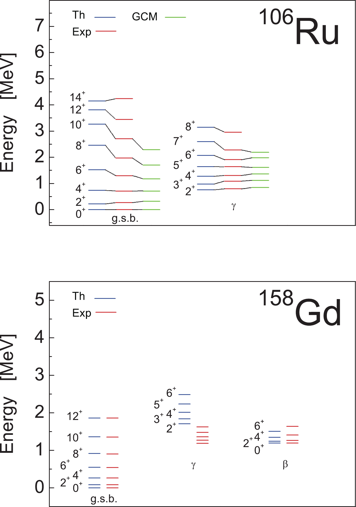
Figure 3. (color online) Comparison of the excitation energies of the ground and
$ \gamma $ bands in$ ^{106} {\rm{Ru}}$ and those of the ground,$ \beta $ , and$ \gamma $ bands in$ ^{158} {\rm{Gd}}$ via experiments according to Eqs. (67) and (70). The values of the model parameters in MeV are as follows:$ A = 0 $ ,$ B = -0.0924 $ ,$ a = 0.004 $ ,$ b = 0 $ , and$ h = -0.23 $ for$ ^{106} {\rm{Ru}}$ and$ A = 0 $ ,$ B = -0.0127 $ ,$ a = 0.0134 $ ,$ b = 0.0000093 $ , and$ h = -0.1384 $ for$ ^{158} {\rm{Gd}}$ , respectively. For$ ^{106} {\rm{Ru}}$ , the results of the general collective model (GCM) with a collective potential including terms up to the sixth order are given as well [58].In Figs. 4 and 5 we present the SU(3) decomposition of the wave functions of the ground and
$ \gamma $ bands in$ ^{106} {\rm{Ru}}$ , and the ground,$ \beta $ , and$ \gamma $ bands in$ ^{158} {\rm{Gd}}$ for different angular momentum values. These figures show that the SU(3) symmetry is severely broken; however, the mixing of different SU(3) multiplets is performed in an approximately coherent way in which the squared amplitudes are almost L-independent. This is accurate for the low angular momenta for which the Coriolis and centrifugal forces are not significantly strong, especially for the case of a well deformed nucleus$ ^{158} {\rm{Gd}}$ . An interesting picture for the SU(3) decomposition coefficients is observed for$ ^{158} {\rm{Gd}}$ , which resembles the eigenfunctions of the simple one-dimensional harmonic oscillator given by the Hermite polynomials. Figures 4 and 5 thus indicate a new kind of symmetry, called quasi-dynamical symmetry [59]. This symmetry is associated with the mathematical concept of embedded representations [60]. We also note that all the SU(3) multiplets that contribute to the structure of collective states, for both nuclei, belong to a single SO(6) irreducible representation$ - $ namely that of maximum seniority$ \upsilon_{0} $ of the corresponding bandhead structure. Thus, the results for the microscopic structure of the rotational states of the lowest collective bands in the two nuclei under consideration reveal, in addition to the good SO(6) symmetry, the presence also of an approximate SU(3) quasi-dynamical symmetry for the low angular momenta, in the sense given in Refs. [27, 59].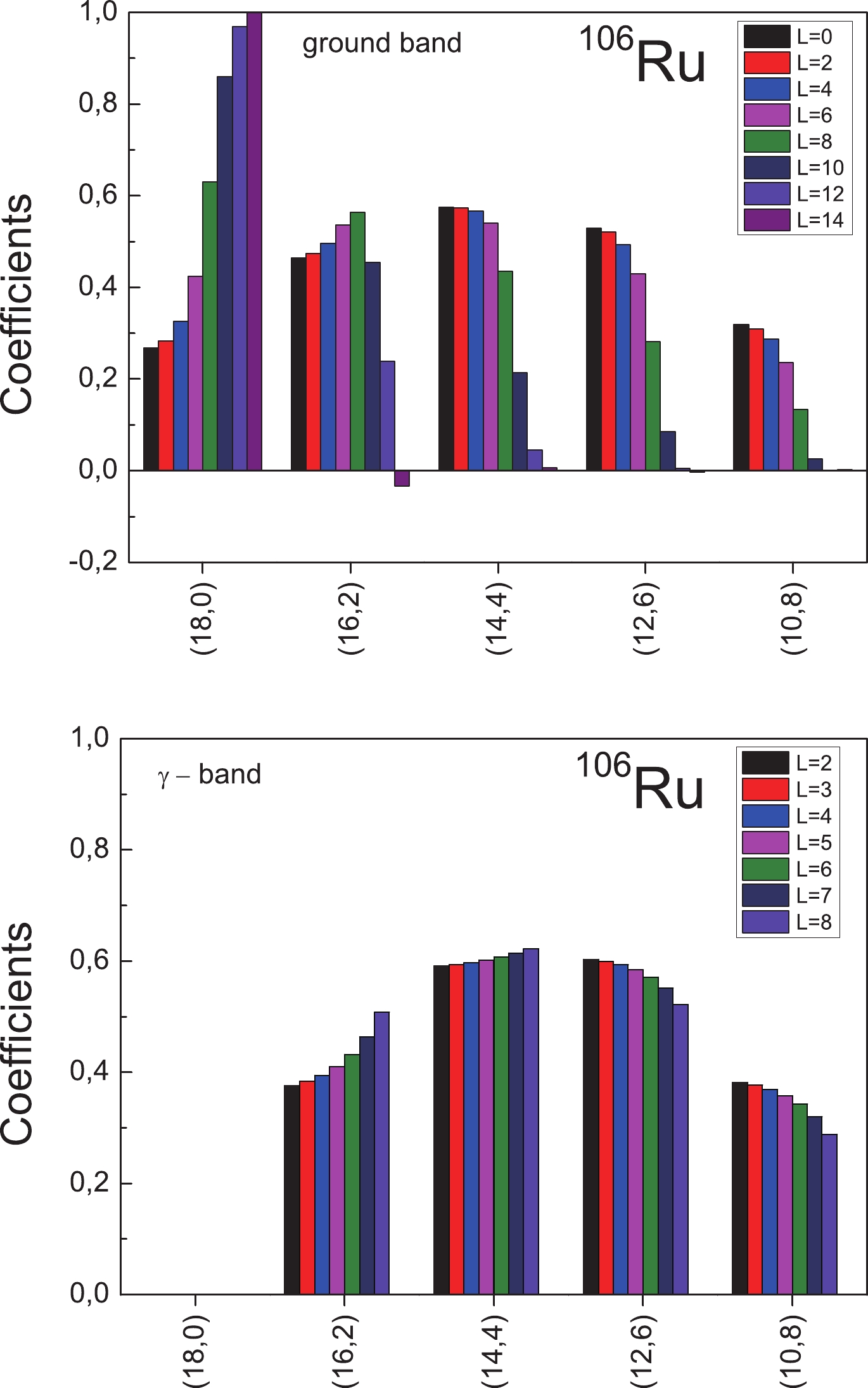
Figure 4. (color online) The SU(3) decomposition of the wave functions of the ground and
$ \gamma $ bands in$ ^{106} {\rm{Ru}}$ for different angular momentum values.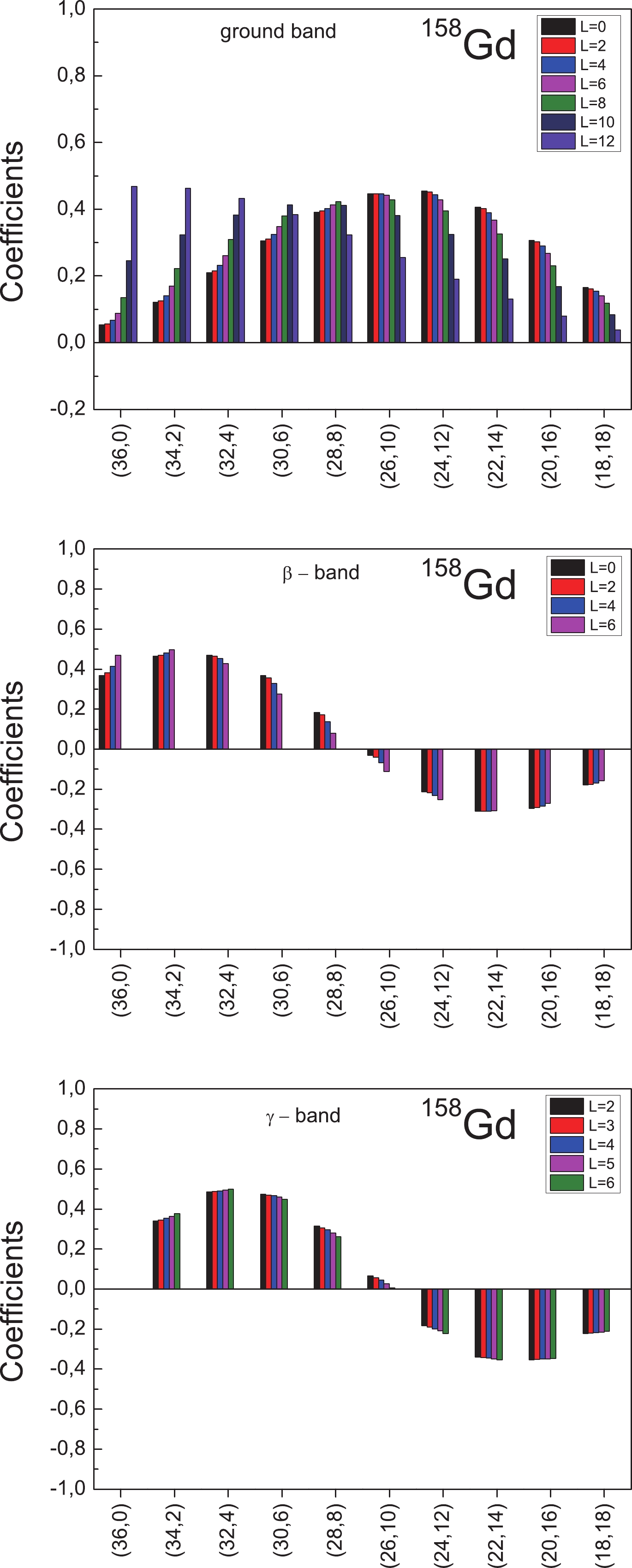
Figure 5. (color online) The SU(3) decomposition of the wave functions of the ground,
$ \beta $ , and$ \gamma $ bands in$ ^{158} {\rm{Gd}}$ for different angular momentum values. -
The purpose of this work is to develop a computational technique for the shell-model reduction chain Sp(12,R)
$ \supset $ SU(1,1)$ \otimes $ SO(6)$ \supset $ U(1)$ \otimes $ SU$ _{pn} $ (3)$ \otimes $ SO(2)$ \supset $ SO(3) of the PNSM. This dynamical symmetry limit was recently shown to correspond to a microscopic shell-model version of the generalized quadrupole-monopole Bohr-Mottelson collective model by embedding the latter in the microscopic shell-model theory [10].The shell-model coupling scheme, defined by the considered reduction chain, provides an alternative basis for the diagonalization of different Hamiltonians of the algebraic and polynomial type in the many-particle position and momentum coordinates of the nuclear system. In the present paper, however, we consider simple algebraic interactions, which are expressed as simple functions of the symplectic generators of Sp(12,R) dynamical group. Closed analytical expressions along the Sp(12,R)
$ \supset $ SU(1,1)$ \otimes $ SO(6)$ \supset $ U(1)$ \otimes $ SU$ _{pn} $ (3)$ \otimes $ SO(2)$ \supset $ SO(3) dynamical symmetry chain are obtained for the matrix elements of the basic building blocks of the PNSM and the Sp(12,R) symplectic generators, which in turn allows computing the matrix elements of other physical operators of interest. In particular, the reduced matrix elements of the tensor operators$ A^{2}(\alpha,\beta)\cdot F^{2}(\alpha,\beta) \simeq [A^{2}(\alpha,\beta)\times $ $ F^{2}(\alpha,\beta)]^{\upsilon = 2}_{\nu = \pm2100} $ and$ F^{2}(\alpha,\beta)\cdot F^{2}(\alpha,\beta) \simeq [F^{2}(\alpha,\beta)\times $ $ F^{2}(\alpha,\beta)]^{4}_{\pm4100} $ , which couple the microscopic shell-model states from different oscillator shells, are also explicitly provided. The matrix elements of other, more complicated interactions can be obtained utilizing the analytical expressions presented here. In this way, the computational technique developed in the present paper generally provides us with the required algebraic tool for performing realistic symplectic-based shell-model calculations of nuclear collective excitations.Two simple examples are given which illustrate the application of the theory to the determination of the microscopic shell-model structure of the observed low-energy rotational states in 106Ru and 158Gd, exhibiting different collectivity in their spectra. The SU(1,1)
$ \otimes $ SO(6) shell-model coupling scheme of the PNSM will extend its applicability in describing the collective properties of different heavy mass nuclei. This variant of the PNSM provides an interesting and relevant framework for exploring the nuclear collective dynamics. More detailed application of the proton-neutron symplectic-based shell-model theory to the description of low-lying excited states in different nuclei with varying collective properties will be presented elsewhere.
Matrix elements in the SU(1,1) ${\otimes}$ SO(6) limit of the proton-neutron symplectic model
- Received Date: 2021-06-30
- Available Online: 2021-11-15
Abstract: The matrix elements along the reduction chain Sp(12,R)


 DownLoad: