


 Abstract
 HTML
HTML Reference
 Related
 PDF
PDF


-
Two-proton (
$ 2p $ ) radioactivity is an exotic decay mode with an emission of two protons from the nuclei near the$ 2p $ drip-line. In 1960, Zel'dovich predicted the possibility that a pair of protons might be emitted from the ground state of a nucleus [1], a phenomenon that was named "$ 2p $ radioactivity" by Goldansky [2, 3]. Due to the proton pairing effect,$ 2p $ radioactivity usually occurs in the even-Z nuclei so that one-proton ($ 1p $ ) radioactivity is strongly forbidden or substantially suppressed. Moreover, during the process of$ 2p $ emission, the energy level of the$ 2p $ emitting channel is lower than that of$ 1p $ radioactivity.$ 2p $ emission is called true$ 2p $ radioactivity and has$Q _{2p}>0 $ and$Q _{p}<0 $ ($Q _{2p} $ and$Q _{p} $ are the released energies of$ 2p $ and$ 1p $ radioactivity, respectively). [4-6]. Although some probable$ 2p $ radioactivity candidates, such as 39Ti, 42Cr, 45Fe, and 48,49Ni, were predicted by various models [2, 3, 7-13],$ 2p $ radioactivity had not been discovered for a long time. More than 40 years later, ground-state true$ 2p $ radioactivity was observed for the first time from 45Fe [14, 15] and then from the ground states of 54Zn [16], 48Ni [17], and 67Kr [18]. So far, ground state$ 2p $ radioactivity with long half-lives has only been observed from those four nuclides. In addition, extremely short-lived$ 2p $ radioactivity from the ground state was observed from 6Be [19], 12O [20-23], 16Ne [21, 24], and 19Mg [25]. For 6Be, 12O, and 16Ne, the decaying states have large widths so that the$ 2p $ emitter states and the$ 1p $ daughter states overlap with each other. Therefore, the decay will most likely take place sequentially [4-6, 26]. However, the situation of 19Mg is less clear because the structure and mass of 18Na (its$ 1p $ daughter nucleus) are experimentally unobtainable. The wave function is more confined in the nuclear interior because of its stronger Coulomb barrier, which causes the narrower decay states.In addition to ground state
$ 2p $ radioactivity,$ 2p $ emission may take place from the excited states. In 1980, Goldansky predicted that$ \beta $ -delayed$ 2p $ ($ \beta 2p $ ) radioactivity candidates could be found in the$ \beta 2p $ emitters of Z = 10~20 [27]. Shortly after that, the$ \beta 2p $ radioactivity of 22Al was observed for the first time in the Lawrence Berkeley National Laboratory [28]; subsequently, more$ \beta 2p $ nuclei, such as 23Si [29], 26P [30], 27S [31], 31Ar [32], 35Ca [33], 39Ti [34], 43Cr [35, 36], and 50Ni [37] were discovered. In addition to populating excited$ 2p $ emitter states with$ \beta $ decays, some$ 2p $ emitters (14O [38], 17,18Ne [39-43], 22Mg [44, 45], and 28,29S [46, 47]) were discovered from the excited states fed by nuclear reactions such as pick up, transfer, and fragmentation reactions. Recently, the$ 2p $ -radioactive decay from an abnormal, spinning, and long-lived state of 94Ag was reported for the first time by Mukha et al. [48].To understand the mechanism of
$ 2p $ radioactivity, several microscopic and phenomenological models have been proposed [10, 11, 49-73]. Generally, the mechanisms are divided into the following three types [5, 6]: (i) 2He cluster emission, (ii) three-body emission, and (iii) sequential emission. In 2He cluster emission, the two protons are strongly correlated and constitute a quasi-bound 1S0 configuration with a very short lifetime. Then, such a quasi-bound state becomes separated after penetrating the Coulomb barrier. For three-body emission, the nuclear core and the two protons separate simultaneously, and the two protons are only relevant to the final correlation and are emitted from the parent nucleus. For sequential emission, the initial nucleus first decays to an intermediate state via the emission of a proton; by subsequently emitting the other proton from the intermediate state, the final state is formed. Hence, sequential emission can be seen as twice$ 1p $ sequential emission. Because the nucleon wave function configurations and the nucleon-nucleon interaction are involved in the two correlated protons, the first two mechanisms attract the interests of researchers. Furthermore, the study of$ 2p $ radioactivity is significant for nuclear astrophysics. For example,$ 2p $ radioactivity is highly relevant to the (2p,$ \gamma $ ) and ($ \gamma $ , 2p) processes of stellar evolution, which are important for studying the nuclear characteristics at waiting-points [74]. Thus, studies on the structures and properties of the$ 2p $ radioactivity nuclei become an important frontier in modern nuclear physics.It is well known that
$ 1p $ ,$ \alpha $ , and cluster radioactivity are important decay modes for unstable nuclei. These emissions can be regarded as super-asymmetric quasi-fission processes of nuclei; therefore, they can be described by a universal approach based on nuclear fission theory. The unified fission model (UFM) can accurately predict the half-lives of these types of radioactivity [75-81]. From this, we consider whether$ 2p $ radioactivity can be studied and described by the UFM if the two emitted protons are seen as a 2He cluster. Therefore, it is interesting to extend the UFM to study 2p radioactivity. This constitutes the motivation of our article, which is organized as follows. In Sec. II, the theoretical framework of the UFM is introduced. In Sec. III, the calculated results and relevant discussions are presented. In the last section, the conclusions are summarized. -
In this study, the UFM we used is a modified version of the preformed cluster model proposed by Gupta and collaborators [75-77]. In the framework of the UFM, the
$ 2p $ -pair with zero binding energy is preformed near the nuclear surface and separates quickly due to the dominance of the Coulomb repulsion after escaping from the barrier.The half-life is expressed as
$ T_{2p} = \frac{\ln 2}{S_{2p}\nu _{0}P}, $

(1) where
$ S_{2p} $ is the preformation factor of the 2He cluster, which is similar to the preformation factor of an$ \alpha $ -particle in the$ \alpha $ -decay process or the spectroscopic factor of$ 1p $ radioactivity. It can be estimated using the cluster overlap approximation [11]$ S_{2p} = G^{2}[A_{0}/(A_{0}-2)]^{2n}\chi ^{2}. $

(2) Here,
$ G^{2} = (2n)!/[2^{2n}(n!)^{2}] $ [82], and$ n $ is the average principal proton oscillator quantum number given by$ n \approx (3Z_{0})^{1/3}-1 $ [83].$ A_{0} $ and$ Z_{0} $ are the mass number and charge number of the parent nucleus, respectively.$ \chi ^{2} $ is the proton overlap function, which is determined by fitting the experimental$Q _{2p} $ values and half-lives [57].$ \nu _{0} $ is the assault frequency of the$ 2p $ -pair on the barrier of the parent nucleus and is estimated by the following classical method:$ \nu _{0} = \frac{1}{2R_0}\sqrt{\frac{2E_{2p}}{M_{2p}}}, $

(3) where R0 is the radius of the parent nucleus.
$ E_{2p} $ and$ M_{2p} $ represent the kinetic energy and the mass of the emitted$ 2p $ -pair, respectively.The penetrability
$ P $ is calculated by the WKB approximation, which is expressed as$ P = \exp \left[ -\frac{2}{\hbar }\int_{R_{\rm in}}^{R_{\rm out}}\sqrt{2\mu (V(r)-Q_{2p})}{\rm d}r \right], $

(4) where
$R _{\rm{in}} $ and$ R_{\rm{out}} $ are the first and second turning points, respectively, with V($R _{\rm in}$ ) = V$(R_{\rm out})$ = Q2p.$ \mu $ is the reduced mass of the$ 2p $ -pair and the residual daughter nucleus. The potential V(r) is parameterized simply as a polynomial for$r \leqslant R_{1}+R_{2} $ , which is expressed as$ V(r) = a_{0}+a_{1}r+a_{2}r^{2}, $

(5) where the coefficients a0, a1, and a2 are determined by the following boundary conditions:
(i) At r = R0 =
$ R_{in} $ , V(r) = Q2p;(ii) At r =
$ R_{1}+R_{2} $ ,$ V(r) = V(R_{1}+R_{2}) $ ;(iii) At r =
$ R_{1}+R_{2} $ ,$ V^{{\prime }}(r) = V^{{\prime }}(R_{1}+R_{2}) $ .Here, R1 and R2 are the radii of the daughter nucleus and the emitted cluster, respectively. The radii measured in fm are given by
$ R_{i} = (1.28A_{i}^{1/3}-0.76+0.8A_{i}^{-1/3}),i = 0,1,2. $

(6) However, for
$r \geqslant R_{1}+R_{2} $ , V(r) is composed of the repulsive Coulomb potential, attractive proximity potential, and centrifugal potential and is written as$ V(r) = V_{p}(r)+V_{l}(r)+\frac{Z_{1}Z_{2}e^{2}}{r}, $

(7) where Z1 and Z2 are the charge numbers of the emitted particle and daughter nucleus, respectively.
$ V_{p} $ is an additional attraction due to the nuclear proximity potential, whose form can be found in Refs. [76, 77, 79-81]. The centrifugal potential$ V_{l}(r) $ due to the angular momentum of the emitted$ 2p $ -pair (l) takes the following form:$ V_{l}(r) = \frac{l(l+1)\hbar ^{2}}{2\mu r^{2}}. $

(8) -
The
$ 2p $ radioactivity half-lives of the ground-state to ground-state transitions are calculated within the UFM by inputting the experimental$Q _{2p} $ values. In Table 1, column 1 contains the$ 2p $ emitters, and column 2 shows the experimental$Q _{2p} $ values. From calculations, the adjustable parameter$ \chi ^{2} $ is determined as 0.038 by fitting the experimental$Q _{2p} $ values and half-lives; hence, the$ S_{2p} $ values can be obtained using Eq. (2), which are shown in column 3. The experimental and the calculated logarithm half-lives within the UFM, the generalized liquid drop model (GLDM) [57], the effective liquid drop model (ELDM) [58], and the Gomow-like model [59] are listed in the 4th-8th columns. The error bars of the calculated half-lives in columns 4 and 5 result from the errors of the experimental$Q _{2p} $ values. Note that for$ 2p $ radioactivity of these nuclei, the l values are all zero. Therefore, the centrifugal potential contribution to the half-life vanishes. In order to analyze the deviation of the experimental half-lives from the calculated ones, the values of the logarithm hindrance factor$ \log_{10}HF $ ($ \log_{10}HF = \log_{10}T_{1/2}^{\rm{expt.}}- \log_{10}T_{1/2}^{\rm{UFM}} $ ) are listed in the final column of Table 1. From Table 1, an agreement between the calculated half-lives and the experimental data is found. Furthermore, it can be seen that the calculated half-lives within the UFM are similar to those within the three other models. Hence, the UFM can be considered to have a comparable accuracy to that of the other models.Nuclei $Q _{2p}^{\text{expt.}} /{\rm{MeV}}$ 

$ S_{2p} $ 

$ \log_{10}T_{1/2}^{\text{2p}}/{\rm s} $ 

$ \log_{10}HF $ 

Expt. UFM GLDM [57] ELDM [58] Gamow-like [59] UFM $ ^{6}_{4}{\rm{Be}} $ 

1.371(5) [19] 0.043 $-20.30 _{-0.03}^{+0.03} $ [19]

$-19.41 _{-0.003}^{+0.003} $ 

$-19.37 _{-0.01}^{+0.01} $ 

−19.97 −19.70 −0.89 $ ^{12}_{8} {\rm{O}}$ 

1.638(24) [20] 0.030 >−20.20 [20] $-18.45 _{-0.03}^{+0.04} $ 

$-19.17 _{-0.08}^{+0.13} $ 

−18.27 −18.04 >−1.75 1.820(120) [21] 0.030 $-20.94 _{-0.21}^{+0.43} $ [21]

$-18.69 _{-0.14}^{+0.15} $ 

$-19.46 _{-0.07}^{+0.13} $ 

−18.30 −2.25 1.790(40) [22] 0.030 $-20.10 _{-0.13}^{+0.18} $ [22]

$-18.65 _{-0.05}^{+0.05} $ 

$-19.43 _{-0.03}^{+0.04} $ 

−18.26 −1.45 1.800(400) [23] 0.030 $-20.12 _{-0.26}^{+0.78} $ [23]

$-18.66 _{-0.41}^{+0.62} $ 

$-19.44 _{-0.20}^{+0.30} $ 

−18.27 −1.46 $ ^{16}_{10}{\rm{Ne}} $ 

1.330(80) [21] 0.024 $-20.64 _{-0.18}^{+0.30} $ [21]

$-16.49 _{-0.22}^{+0.24} $ 

$-16.45 _{-0.21}^{+0.23} $ 

−16.23 −4.15 1.400(20) [24] 0.024 $-20.38 _{-0.13}^{+0.20} $ [24]

$-16.68 _{-0.05}^{+0.05} $ 

$-16.63 _{-0.05}^{+0.05} $ 

−16.60 −16.43 −3.70 $ ^{19}_{12}{\rm{Mg}} $ 

0.750(50) [25] 0.022 $-11.40 _{-0.20}^{+0.14} $ [25]

$-11.77 _{-0.43}^{+0.47} $ 

$-11.79 _{-0.42}^{+0.47} $ 

−11.72 −11.46 0.37 $ ^{45}_{26}{\rm{Fe}} $ 

1.100(100) [14] 0.016 $-2.40 _{-0.26}^{+0.26} $ [14]

$-1.94 _{-1.18}^{+1.34} $ 

$-2.23 _{-1.17}^{+1.34} $ 

−2.09 −0.46 1.140(50) [15] 0.016 $-2.07 _{-0.21}^{+0.24} $ [15]

$-2.43 _{-0.58}^{+0.61} $ 

$-2.71 _{-0.57}^{+0.61} $ 

−2.58 0.36 1.154(16) [17] 0.016 $-2.55 _{-0.12}^{+0.13} $ [17]

$-2.60 _{-0.18}^{+0.19} $ 

$-2.87 _{-0.18}^{+0.19} $ 

−2.43 −2.74 0.05 1.210(50) [84] 0.016 $-2.42 _{-0.03}^{+0.03} $ [84]

$-3.23 _{-0.52}^{+0.56} $ 

$-3.50 _{-0.52}^{+0.56} $ 

−3.37 0.81 $ ^{48}_{28}{\rm{Ni}} $ 

1.290(40) [85] 0.015 $-2.52 _{-0.22}^{+0.24} $ [85]

$-2.29 _{-0.41}^{+0.44} $ 

$-2.62 _{-0.42}^{+0.44} $ 

−2.59 −0.23 1.350(20) [17] 0.015 $-2.08 _{-0.78}^{+0.40} $ [17]

$-2.91 _{-0.19}^{+0.21} $ 

$-3.24 _{-0.20}^{+0.20} $ 

−3.21 0.83 1.310(40) [86] 0.015 $-2.52 _{-0.22}^{+0.24} $ [87]

$-2.50 _{-0.41}^{+0.43} $ 

$-2.83 _{-0.41}^{+0.43} $ 

−2.36 0.015 −0.02 $ ^{54}_{30} {\rm{Zn}}$ 

1.280(210) [88] 0.015 $-2.76 _{-0.14}^{+0.15} $ [88]

$-0.52 _{-2.18}^{+2.80} $ 

$-0.87 _{-0.24}^{+0.25} $ 

−0.93 −2.24 1.480(20) [16] 0.015 $-2.43 _{-0.14}^{+0.20} $ [16]

$-2.61 _{-0.19}^{+0.19} $ 

$-2.95 _{-0.19}^{+0.19} $ 

−2.52 −3.01 0.18 $ ^{67}_{36}{\rm{Kr}}$ 

1.690(17) [18] 0.013 $-1.70 _{-0.02}^{+0.02} $ [18]

$-0.54 _{-0.16}^{+0.16} $ 

$-1.25 _{-0.16}^{+0.16} $ 

−0.06 −0.76 −1.16 Table 1. Comparison between the experimental
$ 2p $ radioactivity half-lives of the ground states and those within different models. The$ Q_{2p}^{\text{expt.}} $ and$\log _{10}T_{1/2} $ values are measured in MeV and s, respectively.Encouraged by the success of the UFM, we attempt to predict the half-lives of the most probable
$ 2p $ decay candidates within it. In our recent study [89], we predicted the half-lives of the most probable$ 2p $ decay candidates within the GLDM by inputting the$Q _{2p} $ values extracted from the mass tables of the Weizsäcker-Skyrme-4 model [90], the finite-range droplet model [91], the Koura-Tachibana-Uno-Yamada model [92], and the Hartree-Fock-Bogoliubov mean-field model with the BSk29 Skyrme interaction [93]. It was shown that the uncertainties of the$ 2p $ decay half-lives are rather large due to the strong model dependence of the$Q _{2p} $ values; and therefore, accurate$Q _{2p} $ values are crucial for predicting the$ 2p $ radioactive half-lives. Thus, the newest$Q _{2p} $ values ($Q _{2p}\approx -S_{2p}^{\prime } $ , where$ S_{2p}^{\prime } $ refers to the two-proton separation energy) from the AME2020 table [94] (See column 2 of Table 2) are used for predicting the$ 2p $ radioactive half-lives. The$S _{2p} $ values given by Eq. (2) and the l values are shown in columns 3 and 4 of Table 2, respectively. Note that the l values are determined by the spin-parity selection rule, and the spin and parity values of the initial and final states are taken from the NUBASE2020 table [95]. The predicted$ 2p $ radioactive half-lives within the UFM are shown in column 5 of Table 2. In addition, the half-lives are predicted within the GLDM and ELDM with the methods used in Refs. [57-89], which are listed in the last two columns of Table 2. Table 2 shows that the majority of the half-lives within the different models are similar to one another. In these models,$ 2p $ radioactivity is treated as a process in which a 2He cluster is first preformed on the nuclear surface and then penetrates the barrier between the 2He cluster and the daughter nucleus. Thus, these models share the same mechanism which leads to similar half-lives. Since the mechanism of$ 2p $ radioactivity is similar to that of$ \alpha $ -decay [96-100], the cluster-like or fission-like models that can describe$ \alpha $ -decay can reproduce the experimental half-lives of$ 2p $ radioactivity. Recently, an extended constraint criterion on the half-life, -12<$\log_{10}T_{1/2}^{\rm{2p}} $ <2 s, was proposed to identify the most probable$ 2p $ decay candidates [89] for future experiments, based on the work of Olsen et al. [62]. According to the constraint condition, the most probable$ 2p $ decay candidates listed in Table 2 are 24P, 39Ti, 40V, 42Cr, 43Mn, 47Co, 49Ni, 56,57Ga, 58,59Ge, 60,61As, 63Se, 65,66Br, and 68Kr.Nuclei $Q _{2p}/{\text{MeV} }$ 

$ S_{2p} $ 

l $\log _{10}T_{1/2}^{\text{2p} }/{\text{s} }$ 

UFM GLDM ELDM $ ^{5}_{4} {\rm{Be}}$ 

7.63 0.053 0 −20.58 − − $ ^{6}_{5} {\rm{B}}$ 

7.42 0.043 0 −20.41 − − $ ^{7}_{5} {\rm{B}}$ 

1.42 0.037 0 −19.33 − −19.19 $ ^{8}_{6} {\rm{C}}$ 

2.11 0.045 0 −19.80 − −19.26 $ ^{10}_{7} {\rm{N}}$ 

1.30 0.035 1 −18.07 −17.98 −17.28 $ ^{11}_{8} {\rm{O}}$ 

4.25 0.032 0 −19.67 − −19.67 $ ^{13}_{9} {\rm{F}}$ 

3.09 0.028 0 −19.33 − −18.89 $ ^{14}_{9} {\rm{F}}$ 

0.05 0.026 1 12.22 − 12.31 $ ^{15}_{10} {\rm{Ne}}$ 

2.52 0.025 0 −18.57 −18.48 −18.08 $ ^{17}_{11} {\rm{Na}}$ 

3.57 0.024 0 −18.95 − −18.63 $ ^{22}_{14} {\rm{Si}}$ 

1.58 0.021 0 −14.61 −18.87 −14.15 $ ^{24}_{15} {\rm{P}}$ 

1.24 0.020 4 −8.50 −9.41 −8.44 $ ^{26}_{16} {\rm{S}}$ 

2.36 0.019 0 −16.09 −19.64 −15.15 $ ^{28}_{17} {\rm{Cl}}$ 

2.72 0.019 2 −15.29 −15.66 −14.47 $ ^{29}_{17} {\rm{Cl}}$ 

0.10 0.018 0 28.91 − 29.44 $ ^{29}_{18} {\rm{Ar}}$ 

5.90 0.018 0 −18.99 − −18.35 $ ^{30}_{18} {\rm{Ar}}$ 

3.42 0.018 0 −17.02 −19.66 −16.15 $ ^{31}_{19} {\rm{K}}$ 

5.66 0.018 2 −18.21 −18.55 −17.29 $ ^{32}_{19} {\rm{K}}$ 

2.74 0.017 2 −14.44 −14.78 −13.68 $ ^{33}_{20} {\rm{Ca}}$ 

5.13 0.017 0 −18.11 −18.48 −17.35 $ ^{34}_{20} {\rm{Ca}}$ 

2.51 0.017 0 −14.46 −14.78 −13.56 $ ^{35}_{21} {\rm{Sc}}$ 

4.98 0.017 3 −16.10 −16.63 −15.57 $ ^{37}_{21} {\rm{Sc}}$ 

0.38 0.017 3 10.92 10.10 10.97 $ ^{37}_{22} {\rm{Ti}}$ 

5.40 0.017 0 −17.81 −17.96 −17.07 $ ^{38}_{22} {\rm{Ti}}$ 

3.24 0.016 0 −15.18 −15.38 −14.30 $ ^{39}_{22} {\rm{Ti}}$ 

1.06 0.016 0 −5.41 −5.55 −4.64 $ ^{39}_{23} {\rm{V}}$ 

4.21 0.016 0 −16.34 −16.54 −15.49 $ ^{40}_{23} {\rm{V}}$ 

2.14 0.016 0 −11.66 −11.80 −10.80 $ ^{41}_{24} {\rm{Cr}}$ 

3.33 0.016 0 −14.53 −14.72 −13.66 $ ^{42}_{24} {\rm{Cr}}$ 

1.48 0.016 0 −7.40 −7.56 −6.66 $ ^{43}_{25} {\rm{Mn}}$ 

2.48 0.016 2 −10.65 −11.03 −10.16 $ ^{44}_{25} {\rm{Mn}}$ 

0.50 0.016 0 9.80 9.51 10.22 $ ^{47}_{27} {\rm{Co}}$ 

1.02 0.015 2 1.13 0.63 1.37 $ ^{49}_{28} {\rm{Ni}}$ 

1.08 0.015 0 0.23 −0.08 0.67 $ ^{52}_{29} {\rm{Cu}}$ 

1.13 0.015 4 3.45 2.70 3.34 $ ^{55}_{30} {\rm{Zn}}$ 

0.78 0.015 2 8.77 8.26 8.92 $ ^{56}_{31} {\rm{Ga}}$ 

2.82 0.014 0 −10.30 −10.83 −9.14 $ ^{57}_{31} {\rm{Ga}}$ 

1.65 0.014 2 −3.01 −3.81 −2.20 $ ^{58}_{31} {\rm{Ga}}$ 

0.51 0.014 2 18.71 17.88 19.33 Continued on next page Table 2. Predicted
$ 2p $ decay half-lives within the UFM, GLDM, and ELDM found by inputting the newest$ Q_{2p} $ values taken from the AME2020 table [94].Table 2-continued from previous page Nuclei $Q _{2p}/{\text{MeV} }$ 

$ S_{2p} $ 

l $\log _{10}T_{1/2}^{\text{2p} }/{\text{s} }$ 

UFM GLDM ELDM $ ^{58}_{32} {\rm{Ge}}$ 

3.23 0.014 0 −11.19 −11.73 −10.02 $ ^{59}_{32} {\rm{Ge}}$ 

1.60 0.014 0 −2.73 −3.37 −1.76 $ ^{60}_{33} {\rm{As}}$ 

3.32 0.014 4 −8.37 −9.34 −7.81 $ ^{61}_{33} {\rm{As}}$ 

1.98 0.014 0 −4.95 −5.61 −3.97 $ ^{62}_{33} {\rm{As}}$ 

0.59 0.014 2 17.99 17.14 18.58 $ ^{63}_{34} {\rm{Se}}$ 

2.36 0.013 0 −6.59 −7.22 −5.60 $ ^{64}_{34} {\rm{Se}}$ 

0.70 0.013 0 14.39 13.69 15.14 $ ^{65}_{35} {\rm{Br}}$ 

2.43 0.013 2 −5.55 −6.37 −4.76 $ ^{66}_{35} {\rm{Br}}$ 

1.39 0.013 0 1.83 1.12 2.68 $ ^{68}_{36} {\rm{Kr}}$ 

1.46 0.013 0 1.83 1.13 2.65 $ ^{81}_{42} {\rm{Mo}}$ 

0.73 0.013 0 23.26 22.67 23.82 $ ^{85}_{44} {\rm{Ru}}$ 

1.13 0.013 0 14.08 13.76 14.66 $ ^{108}_{54} {\rm{Xe}}$ 

1.01 0.012 0 27.07 26.37 27.47 In addition to the mentioned models, two analytical formulas that estimate the ground state
$ 2p $ radioactivity half-lives were recently proposed by extending the empirical formulas for$ 1p $ radioactivity based on the Geiger-Nuttall law [60, 61], which are denoted as the formula of Sreeja and the formula of Liu in this article. Sreeja's formula is expressed as [60]$ \log _{10}T_{1/2} = (al+b)\xi +cl+d, $

(9) where
$ \xi = Z_{d}^{0.8}Q_{2p}^{-1/2} $ , with$ Z_{d} $ being the charge of the daughter nucleus. a, b, c and d are the fitting parameters, which are obtained by fitting the$ 2p $ decay half-lives estimated by the ELDM. These parameters are a = 0.1578, b = 1.9474, c = −1.8795, and d = −24.847, respectively. Liu's formula is written as [61]$ \log _{10}T_{1/2} = a^{\prime }(Z_{d}^{0.8}+l^{\beta })Q_{2p}^{-1/2}+b^{\prime}, $

(10) where the adjustable parameters
$ a^{\prime } $ ,$ b^{\prime } $ , and$ \beta $ , whose values are 2.032, −26.832, and 0.25, respectively, are obtained by fitting the experimental data and the calculated results based on the ELDM. Here$ \beta $ reflects the effect of the angular momentum on the$ 2p $ radioactivity half-lives.Although the estimated ground state
$ 2p $ decay half-lives within the UFM and the two formulas are in good agreement with the experimental values, their reliability needs to be tested with more experimental data. Some experimental$ 2p $ decay half-lives of the excited states have been accumulated in recent decades, which can be used for ground testing the validity of the UFM and the two formulas. Thus, the UFM and Eqs. (9, 10) are extended to study the excited states. In Table 3, the$ 2p $ transitions from the excited states to either the ground states or excited states are listed in column 1. The initial and final spin-parity values are given in column 2 and column 3, respectively. In columns 4-6, the l values, the$Q _{2p} $ values, and the experimental logarithm half-lives are listed. The l values are extracted by the spin-parity selection rule and are selected to be zero for the cases of 22Mg* and 29S* because the spin-parity of their initial states has not been determined experimentally. As for 94Ag*, the l value was conservatively estimated to be between 6 and 10$ \hbar $ by assuming that the un-assigned$ \gamma $ -rays may take up to$ 4\hbar $ of angular momentum [48]. Therefore, in our calculations,$l = 6 \sim 10 \hbar $ is used. Note that, in calculations, the$ S_{2p} $ values of the excited states are assumed to be the same as those of the ground states. The calculated logarithm half-lives within the UFM, Sreeja's formula, and Liu's formula are listed in columns 7-9. In addition, the half-lives extracted from other models are listed in the final column.Transitions $ J_{i}^{\pi } $ 

$ J_{f}^{\pi } $ 

l $ Q_{2p} $ /MeV

$\log _{10}T_{1/2}^{\text{2p}} $ /s

Expt. UFM Sreeja Liu Other $_{8}^{14} {\rm{O} } ^{\ast }\longrightarrow _{6}^{12}{\rm C}+2p$ 

2+ 0+ 2 1.20[38] >−16.12[38] −16.02 −19.94 −16.85 −18.12[38] (2)+ 0+ 2 3.15[38] −18.87 −23.26 −20.67 4+ 0+ 4 3.35[38] −15.96 −26.46 −20.61 $_{10}^{17} {\rm{Ne} } ^{\ast }\longrightarrow _{8}^{15}{\rm O}+2p$ 

3/2− 1/2− 2 0.35[39,40] >−10.59[40] −7.11 −8.42 −4.62 −9.40[11] 3/2− 1/2− 2 0.35[39,40] −6.89[52] 3/2− 1/2− 2 0.35[39,40] $ -6.33_{-0.10}^{+0.09} $ [64]

5/2− 1/2− 2 0.82[39,40] −12.73 −15.42 −12.32 1/2+ 1/2− 1 0.97[39,40] −14.69 −15.44 −13.88 $_{10}^{18}{\rm{Ne} } ^{\ast }\longrightarrow _{8}^{16}{\rm O}+2p$ 

2+ 0+ 2 0.59[42] −10.91 −13.06 −9.72 1− 0+ 1 1.63[42] $ -16.15_{-0.06}^{+0.06} $ [42,43]

−16.79 −18.02 −16.84 −17.12[42] $_{12}^{22} {\rm{Mg} } ^{\ast }\longrightarrow _{10}^{20}{\rm Ne}+2p$ 

− 0+ 0 6.11[44,45] −18.97 −19.88 −21.65 $_{16}^{29} {\rm{S} } ^{\ast }\longrightarrow _{14}^{27}{\rm Si}+2p$ 

− 5/2+ 0 1.72~2.52[46] −16.4~−14.3 −14.7~−12.6 −16.3~−14.0 − 5/2+ 0 4.32~5.12[46] −18.9~−18.5 −17.7~−17.1 −19.4~−18.8 $_{47}^{94} {\rm{Ag} }^{\ast }\longrightarrow _{45}^{92}{\rm Rh}^{\ast }+2p$ 

21+ 11+ 6~10 1.90[48] $1.90 _{-0.20}^{+0.38} $ [48]

9.38~15.21 8.00~10.10 6.46~6.77 4.70[57] 1.98[105] 8.56~14.37 7.10~9.01 5.78~6.09 2.05[105] 7.89~13.68 6.36~8.11 5.22~5.52 3.45[105] −0.92~4.56 −3.75~−3.38 −-2.13~−1.89 Table 3. Comparison between the experimental
$ 2p $ radioactivity half-lives of the excited states and those within different models and formulas. The half-lives that are not available experimentally are also predicted. The symbol "*" represents the excited state of a nucleus.In the next paragraphs,
$ 2p $ radioactivity of the excited states will be discussed by analyzing the calculated results in Table 3. For 14O*, a weak$ 2p $ decay branch with$ \Gamma = 125 \pm 20 $ eV via the 2+ state (E* = 7.77 MeV, E* is the excitation energy) was observed which occurs predominantly by a sequential mechanism [38]. However, an upper limit of the 2He emission$\Gamma _{^{2}{\rm He}} < 6$ eV was measured [38], which corresponds to$\log_{10}T_{1/2}^{2p}$ >−16.12 s. By comparing the measured half-life with those estimated by the UFM, Sreeja's formula, Liu's formula, and R-matrix theory [38], it is shown that only the half-life within the UFM is larger than the experimental lower limit. For 17Ne*, the$ 2p $ decays from its first two excited states (${3}/{2}^{-}$ and${5}/{2}^{-}$ states) were studied using intermediate energy Coulomb excitation combined with$ 2p $ spectroscopy [40] and a previously performed$ \gamma $ spectroscopy experiment [39]. It was found that the${5}/{2}^{-}$ state (E* = 1.764 MeV) decays, via the sequential$ 2p $ emission, to the ground state of 15O. However, no evidence of a simultaneous$ 2p $ decay from the first excited${3}/{2}^{-}$ state was observed. A lifetime limit$ \tau _{2p}>26 $ ps ($ \log_{10}T_{1/2}^{\rm{2p}} $ >−10.59 s) of the${3}/{2}^{-}$ state (E* = 1.288 MeV) was obtained. As seen in Table 3, the$ 2p $ decay half-lives of 17Ne* within all the models are in agreement with the corresponding measured half-life. As for 18Ne*, clear evidence of the simultaneous$ 2p $ emission from the 1– state (E* = 6.15 MeV) was observed with the reaction 17F+1H [42]. However, the two extreme decay mechanisms (the 2He emission and direct three-body decay with no final state interactions) were not distinguished by the measured data due to the limited angular coverage. Nevertheless, the$ 2p $ partial width$ \Gamma _{2p} $ was found to be$21 \pm 3 $ eV, when assuming 2He emission, and$ 57\pm 6 $ eV, when assuming three-body decay. Subsequently, new experimental evidence for 2He emission from the 18Ne excited states was observed by a complete kinematical reconstruction of the decay products at the in-Flight Radioactive Ion Beams (FRIBs) facility of the Laboratori Nazionali del Sud (LNS)-Italy [43]. It was found that the 1– state$ 2p $ decay proceeds through 2He diproton resonance (31%) and democratic or virtual sequential decay (69%). By combining the measurements of Gómez del Campo et al. [42] and Raciti et al. [43], it is evident that the real experimental$ \Gamma _{^{2}{\rm He}} $ of the 1– state of 18Ne is$ 6.51\pm 0.93 $ eV, corresponding to a logarithm lifetime of$-16.15 \pm 0.06 $ s. By comparing the experimental half-life with the estimated values from the four approaches ($\log_{10}T_{1/2}^{{2p}}$ = –17.12 s is estimated from a simple R-matrix [42]), the half-life extracted from the UFM is closest to the experimental value.In recent years, measurements of the decay properties of the 21+ high-spin isomer in 94Ag have been performed because its properties are unique within the entire nuclear chart. This isomer state with a high excitation energy of 6.7(5) MeV and a long half-life of 0.39(4) s makes several decay modes possible: a
$ \beta $ decay followed by a$ \gamma $ -ray or proton emission [101, 102], a$ \beta $ -delayed$ \gamma $ ,$ 1p $ and$ 2p $ decays [101-104], direct$ 1p $ and$ 2p $ emissions [48, 105-108], and$ \alpha $ -radioactivity [109]. The$ \beta $ -delayed$ \gamma $ ,$ 1p $ , and$ 2p $ decays from the 21+ isomer have been reported in [101-104], and then, experiments on direct$ 1p $ and$ 2p $ emissions of the 21+ isomer were performed in several labs [48, 105-108]. In 2005, direct$ 1p $ decay of the 21+ isomer into two high-spin daughter states in 93Pd was identified by detecting protons in coincidence with$ \gamma $ -$ \gamma $ correlations and applying$ \gamma $ gates based on known 93Pd levels [106]. A strong quenching of the partial decay width indicates the importance of parent state deformation. One year later, evidence of the simultaneous$ 2p $ emission of the 21+ isomer to an excited state of the daughter nucleus 92Rh was reported [48]. The$ 2p $ branch was characterized by$Q _{2p} $ = 1.9(1) MeV and a decay probability of 0.5(3)% leading to$ T_{1/2}^{2p} $ = 80 s; the$ 2p $ decay behavior and the unexpectedly large probability were explained by assuming a strong prolate deformation of the 21+ isomer. However, the possibility of$ 2p $ decay of the 21+ isomer was questioned by a measurement by Pechenaya et al. [107]. To uncover the nature of this isomer and its possible decay modes, the masses of 93Pd and 94Ag were deduced by measuring the masses of the$ 2p $ decay daughter 92Rh and the$ \beta $ -decay daughter 94Pd of the high-spin isomer in 94Ag with the Penning trap mass spectrometer JYFLTRAP at the Ion-Guide Isotope Separator On-Line [105]. It was found that the$ E^{\ast } $ value of the 21+ isomer is 6.96 (8.36) MeV, when combined with data from the$ 1p $ ($ 2p $ ) decay experiments. This indicates that the$ E^{\ast } $ value of the 21+ isomer has been uncertain. However, using the two different$ E^{\ast } $ values and the AME2003 data, the extracted$Q _{2p} $ values of this isomeric state are 2.05, 3.45, and 1.98 MeV [105]. The corresponding half-lives from the UFM and the formulas of Sreeja and Liu, found by inputting the three$Q _{2p} $ values and the$Q _{2p} $ value in Ref. [48], are listed in the final four lines of Table 3. In calculations, the l values are taken as$ 6\sim 10 \hbar $ as done in the model in Ref. [48]. From Table 3, it is seen that the experimental half-life is reproduced only in the UFM by inputting$Q _{2p} $ = 3.45 MeV. According to the above discussion on$ 2p $ decay of the excited states of 14O, 17Ne, 18Ne, and 94Ag, it is shown that the predictive power of the UFM is stronger than that of the formulas of Sreeja and Liu because more nuclear structure details are included in it. Therefore, the half-lives that are not available experimentally but predicted by the UFM (see Table 3) appear to be more reliable. However, a reinvestigation by Cerny et al. in 2009 found no evidence to support$ 2p $ radioactivity of the long-lived isomer in 94Ag* [108]. Due to these contradictory measurements [48, 105, 107, 108] and the argument between Mukha and Pechenaya [110, 111], it remains a mystery whether$ 2p $ radioactivity exists in the long-lived isomer of 94Ag*. We fully agree with the viewpoint of Ref. [105]: to finally solve this puzzle, direct mass measurements of 93Pd, 94Ag, and 94Ag* (21+) are needed, posing new challenges for the production of these exotic species. The direct mass measurements of these exotic nuclei are expected with the new generation of radioactive beam facilities [112-114].In addition,
$ 2p $ emission was observed from the higher excited states of 17Ne [41] and 18Ne [43]. In 17Ne, a correlated$ 2p $ emission via 2He resonance might be observed from one or several states with an excitation energy above 2 MeV [41]. The$ 2p $ decay of the high-lying states in 18Ne seems to occur predominantly via a democratic or true sequential decay mechanism [43]. However, the two hypotheses have not yet been tested with further experiments. 17,18Ne beams with high intensities can be applied at new radioactive beam facilities, such as the High Intensity heavy-ion Accelerator Facility (HIAF) of China [112], to test these hypotheses in the future. In contrast, it is recommended that some microscopic models, for example, the shell model, should be developed by taking into account necessary physical factors, such as the tensor force [115], three-body force [116], and accurate pairing force [117], to reasonably describe the mechanism of$ 2p $ emission from the excited states.It is well known that the
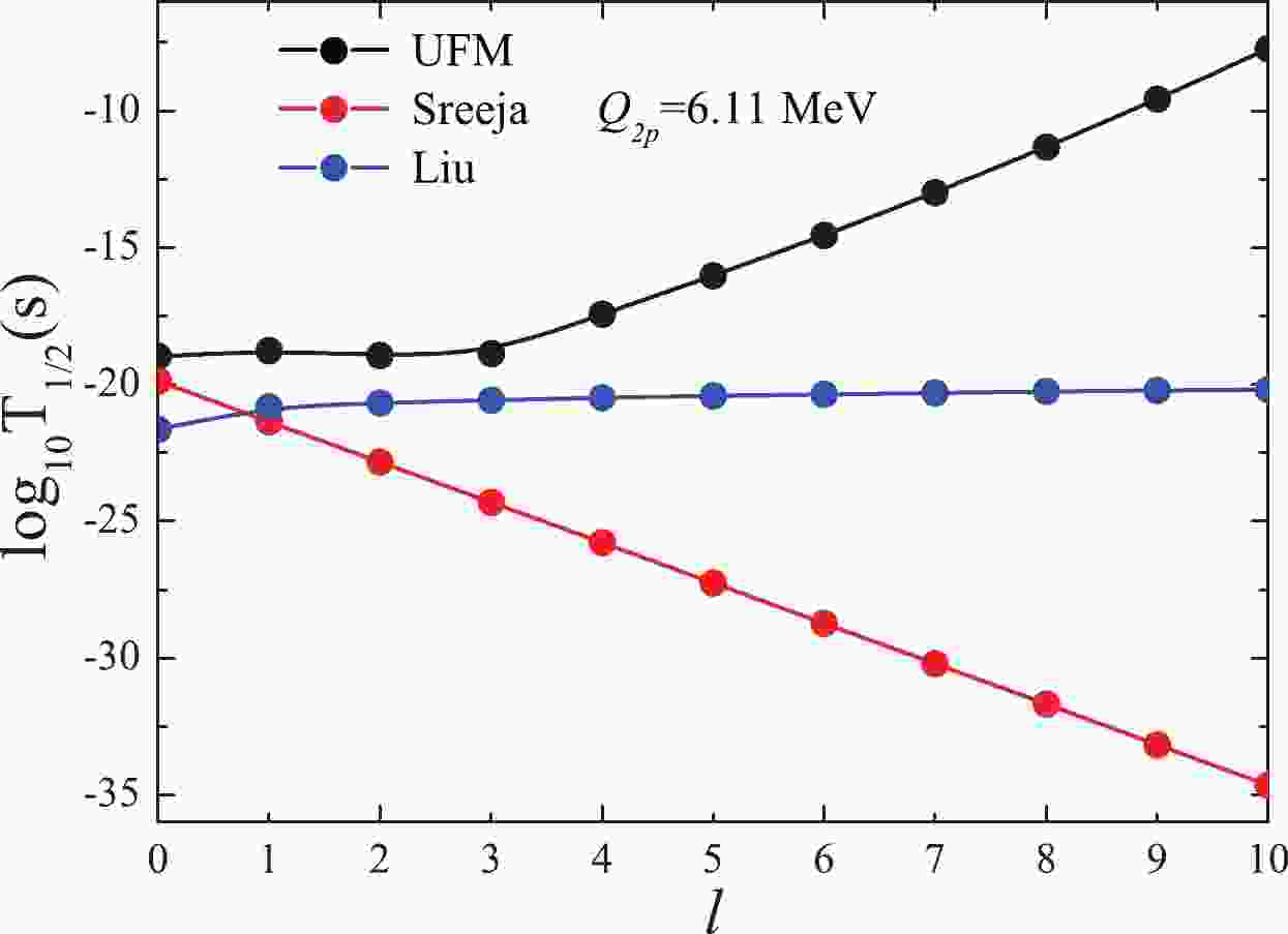
$ 2p $ decay half-life is sensitive to the$Q _{2p} $ and l values [57-61, 89]. Because the$Q _{2p} $ and/or l values of the$ 2p $ decay of 22Mg*, 29S*, and 94Ag* are uncertain, the$ 2p $ decay half-lives of the excited states for the three nuclei versus l, which are obtained by inputting different$Q _{2p} $ values, are plotted in Figs. 1-3. Fig. 1 shows that the$\log_{10}T_{1/2}^{2p}$ curves are very different from one another. For the$ 2p $ decay of 22Mg*,$Z _{d} $ = 10 and$Q _{2p} $ = 6.11 MeV, and the specific forms of Sreeja's formula and Liu's formula are$\log _{10}T_{1/2}({\rm Sreeja}) = -1.477l-19.875$ and$\log _{10}T_{1/2}({\rm Liu}) = $ $ -21.639+0.823l^{0.25}$ , respectively. Thus, the relation between$\log_{10}T_{1/2}^{{2p}}$ and l is linear for Sreeja's formula and non-linear (a power function) for Liu's formula. In the framework of the UFM, the quantity$ \log _{10}T_{1/2}(l>0) $ can be written as [78, 79]
Figure 1. (color online)
$ 2p $ radioactivity half-lives of 22Mg* within the UFM and the formulas of Sreeja and Liu as functions of l.
Figure 2. (color online)
$ 2p $ radioactivity half-lives of 29S* within the UFM and the formulas of Sreeja and Liu by inputting different$Q _{2p} $ values as functions of l.
Figure 3. (color online) Same as Fig. 2, but for the case of 94Ag*. The shaded area represents its experimental half-life.
$ \log _{10}T_{1/2}(l>0) = \log _{10}T_{1/2}(l = 0)+c\frac{l(l+1)}{\sqrt{\mu Z_{1}Z_{2}R_{in}}}, $

(11) where
$ \log _{10}T_{1/2}(l = 0) $ represents the logarithm half-life for the vanishing l, and c is a constant. According to Eq. (11), the relation between$ \log _{10}T_{1/2}(l>0) $ and l is described by a parabolic curve. Similar tendencies can be obtained from the three methods as shown in Figs. 2 and 3. In addition, as shown in Fig. 2(b), the half-lives decrease with the increase in l. For the case of 94Ag*, only the calculated half-lives based on the UFM, with$Q _{2p} $ = 3.45 MeV, are in agreement with the experimental data, as previously discussed during the analysis of Table 3. However, for the formula of Sreeja, the half-lives decrease with l in the case of$Q _{2p} $ = 3.45 MeV, and the evolution trend is the same as that of Fig. 2(b); this is unreasonable because, if l increases, the half-life becomes longer with the increase in the centrifugal barrier. For Liu's formula, although the half-life increases as l increases, this increase is abnormally slow, which can be seen from Figs. 2(c) and 3(c). However, relevant studies indicate that the half-life is clearly enhanced by a large l value, for example, in the case of$ \alpha $ decay [118]. Hence, the two fitting formulas are not suitable for the study of$ 2p $ radioactivity of the excited states. This conclusion is further reinforced by the following. (i) The parameters involved in the two formulas are obtained by fitting a small number of ground state experimental data and/or ground state half-lives within the ELDM by inputting the$Q _{2p} $ values extracted from the AME2016 table [86]. By comparing the AME2016 table [86] and AME2020 table [94], the two types of$Q _{2p} $ values are found to be very different. This leads to a large difference in the half-lives estimated within the ELDM by inputting the two types of$Q _{2p} $ values because the half-lives are sensitive to the$Q _{2p} $ values, which can be seen through a comparison of Table 2 from this article and Table 2 from Ref. [58]. (ii) The experimental data from the excited states are not included in the fitting procedure. If the$Q _{2p} $ values of the AME2020 table are more reliable than those of the AME2016 table, the universal parameters can be obtained by fitting the experimental half-lives of the ground and excited states and the predicted ground state half-lives, within a plausible model, by inputting the$Q _{2p} $ values taken from the AME2020 table. In summary, more nuclear structure information can be obtained by investigating$ 2p $ radioactivity of excited states, which is difficult to observe but worth studying further. -
In this study, the UFM was firstly extended to study the
$ 2p $ radioactivity half-lives of the ground states of nuclei by introducing the parametric spectroscopic factor. The probable$ 2p $ radioactivity candidates of the ground states were predicted within the UFM by inputting the$Q _{2p} $ values from the AME2020 table. Finally,$ 2p $ radioactivity of the excited states of 14O, 17,18Ne, 22Mg, 29S, and 94Ag was discussed using the UFM, Sreeja's formula, and Liu's formula. The obtained results allow us to draw the following conclusions:(i) The calculated half-lives of ground states within the UFM are in good agreement with the experimental values.
(ii) Because the UFM has a similar physical mechanism to the GLDM, ELDM, and Gamow-like model, the predicted half-lives of the ground states within the four models are similar. Furthermore, using the extended half-life constraint condition, the most probable
$ 2p $ decay candidates predicted by the UFM, GLDM, and ELDM are 24P, 39Ti, 40V, 42Cr, 43Mn, 47Co, 49Ni, 56,57Ga, 58,59Ge, 60,61As, 63Se, 65,66Br, and 68Kr.(iii) The experimental
$ 2p $ radioactivity half-lives of the excited states of 14O, 17,18Ne, and 94Ag are reproduced better by the UFM than the formulas of Sreeja and Liu because the former includes more details of nuclear structure. Therefore, the$ 2p $ radioactivity half-lives of the excited states that are not available experimentally but predicted by the UFM are more plausible.(iv) Sreeja's formula and Liu's formula are not suitable for investigating
$ 2p $ radioactivity of the excited states. First, they contradict the fact that the half-life increases as the angular momentum increases. Second, the parameters of the two formulas are obtained only by fitting the$ 2p $ decay data of the ground states and contain no information about the excited states. Thus, to propose a universal formula that estimates the$ 2p $ decay half-lives of both the ground and excited states, more$ 2p $ decay data of ground and excited states should be used in the fitting procedure, which are expected to be measured in a new generation of radioactive beam facilities. -
We thank professor Shangui Zhou, professor Ning Wang, professor Fengshou Zhang, and Dr. Yang Xiao for helpful discussions.
Two-proton radioactivity of ground and excited states within a unified fission model
- Received Date: 2021-07-10
- Available Online: 2021-12-15
Abstract: A unified fission model is extended to study two-proton radioactivity of the ground states of nuclei, and a good agreement between the experimental and calculated half-lives is found. The two-proton radioactivity half-lives of the ground states of some probable candidates are predicted within this model by inputting the released energies taken from the AME2020 table. It is shown that the predictive accuracy of the half-lives is comparable to those of other models. Then, two-proton radioactivity of the excited states of 14O, 17,18Ne, 22Mg, 29S, and 94Ag is discussed within the unified fission model and two analytical formulas. It is found that the experimental half-lives of the excited states are reproduced better within the unified fission model. Furthermore, the two formulas are not suitable for the study of two-proton radioactivity of excited states because their physical appearance deviates from the mechanism of quantum tunneling, and the parameters involved are obtained without including experimental data from the excited states.


 DownLoad: