


 Abstract
 HTML
HTML Reference
 Related
 PDF
PDF


-
Fast radio bursts (FRBs) are short-duration and energetic radio transients, with a typical radiation frequency of
$ \sim $ GHz and a typical duration of$ \sim $ ms, that occur in the Universe. For recent reviews, see Refs. [1-3]. The first discovery of FRBs can be traced back to 2007, when Lorimer et al. reanalyzed the archive data of the Parkes 64-m telescope and found an extraordinary radio pulse, which is now named FRB 010724 [4]. For a long time, this phenomenon did not attract much attention from astronomers, until four other bursts were discovered in 2013 [5]. Since then, FRBs have gained significant interest within the astronomy community. The observed dispersion measures (DM) of most FRBs greatly exceed the contribution from the Milky Way, indicating that they occur at cosmological distances, and the cosmological origin is further confirmed by the identification of the host galaxy and the direct measurement of redshift [6-8]. Owing to the progress in observational techniques, more FRBs have been discovered in recent years, and, to date, hundreds of FRBs have been reported [9, 10]. Generally, FRBs can be divided into two types according to whether they are repeating or not. Most FRBs observed so far are thought to be non-repeating; however, tens of FRBs have been found to be repeating without periodicity. Except for an extremely active repeating source, FRB 121102, from which hundreds of bursts have been detected [11-14], most of the other repeating sources found by the Canadian Hydrogen Intensity Mapping Experiment (CHIME) telescope repeat only two or three times [15]. Statistical analysis of FRB 121102 shows that the burst energies from this source follow the bent power-law and are scale-invariant [16], implying that there are some similarities between FRBs and soft gamma repeaters (SGRs) [17]. Recently, the CHIME/FRB Collaboration [18] found an unexpectedly long period of 16.35 d with an approximately 4-day active window in FRB 180916.J0158+65. Interestingly, the recently discovered FRB 200428 was found to be associated with the Galactic magnetar SGR 1935+2154 [19], which implies that magnetars are the progenitors of at least some FRBs.FRBs are very energetic and detectable up to a high redshift [20]; therefore, they can be used as instruments to study cosmology. Yu & Wang showed that FRBs can be used to measure the cosmic proper distance [21]. Walters et al. showed that FRBs can constrain cosmological parameters, especially the baryon matter density [22]. Li et al. proposed that FRBs can be used to independently constrain the fraction of baryon mass in the intergalactic medium (IGM) model [23, 24]. Xu & Zhang proposed that FRBs can be used to probe intergalactic turbulence [25]. Wu et al. pointed out that FRBs can aid in measuring the Hubble parameter
$ H(z) $ independent of the cosmological model [26]. Pagano & Fronenberg showed that highly dispersed FRBs can be utilized to constrain the epoch of cosmic reionization [27]. Qiang et al. showed that FRBs can be used to test the possible cosmic anisotropy [28]. In addition, the strongly lensed FRBs can be used to investigate compact dark matter in the Universe [29]. Strongly-lensed repeating FRBs can tightly constrain the Hubble constant and cosmic curvature [30] and can be used as probes to search for gravitational waves [31]. Moreover, FRBs can be used to test fundamental physics, such as constraining the weak equivalence principle and photon mass [32-35].Observations of the cosmic microwave background (CMB) show that the Universe is homogeneous and isotropic on a large scale [36, 37]. However, there is no direct evidence that the baryon matter is also isotropic, and observations of the luminosity of type-Ia supernovae show that there is possible anisotropy [38-40]. In addition, observations of the fine-structure constant from quasar absorption lines show that the Universe may be anisotropic [41, 42]. Interestingly, the dipole fitting of both the supernovae data and fine-structure constant data leads to a consistent dipole direction [43], and this anisotropy can be caused by, for example, the interaction of photons with the anisotropic distribution of baryon matter. In this paper, we will show that FRBs can be used to test the possible anisotropic distribution of baryon matter in the Universe. The DM is the integral of electron density along the line of sight, while the latter is proportional to the baryon matter in the Universe. By measuring the DM of hundreds of FRBs in different directions in the sky, we can detect the anisotropic signal in the baryon matter distribution.
The rest of this paper is arranged as follows: In Section II, we present the methodology for testing the anisotropic distribution of baryon matter using FRBs. In Section III, we investigate the capability of future FRB data to test the anisotropic distribution of baryon matters using Monte Carlo simulations. Finally, discussions and conclusions are presented in Section IV.
-
Owing to the interaction between photons and free electrons, photons with different energies travel with different speeds. The relative time delay between low- and high- energy photons propagating from a distant source to Earth is proportional to the DM, which is the integral of electron density along the photon path [44]. This effect is especially important in the low-energy wave bands, such as the radio bands in which FRBs are observed. The DM is related to the matter distribution along the light path; therefore, it contains the information of the Universe and the distance to the FRB source.
In general, the observed DM of an FRB contains three parts: the contributions from the Milky Way (MW), the intergalactic medium (IGM), and the host galaxy [45, 46],
$ {\rm DM_{obs}} = {\rm DM_{MW}}+{\rm DM_{IGM}}+\frac{{\rm DM_{host}}}{1+z}, $

(1) where the factor
$ 1+z $ accounts for the cosmic dilation. The term$ {\rm DM_{MW}} $ can be well constrained by modelling the electron distribution of the MW [47-49], as long as the position of the FRB is known. Thus it can be subtracted from the total observed DM, leaving behind the extragalactic DM,$ {\rm DM_{\it E}}\equiv{\rm DM_{obs}}-{\rm DM_{MW}}. $

(2) The uncertainty of
${{\rm DM}_E}$ is propagated from the uncertainties of$ {\rm DM_{obs}} $ and$ {\rm DM_{MW}} $ , that is,$ \sigma_E = \sqrt{\sigma^2_{\rm obs}+\sigma^2_{\rm MW}} $ .$ {\rm DM_{obs}} $ can be tightly constrained by observing the time-resolved spectra of the FRBs. According to the FRB catalog [9], the average uncertainty on$ {\rm DM_{obs}} $ is only 1.5 pc cm$ ^{-3} $ . For FRBs at high Galactic latitudes$ (|b|>10^\circ) $ , the DM contribution from the MW can be tightly constrained with an average uncertainty of 10 pc cm$ ^{-3} $ [50]. Therefore, we use$ \sigma_{\rm obs} = 1.5\; {\rm pc\; cm}^{-3} $ and$ \sigma_{\rm MW} = $ $ 10\; {\rm pc\; cm}^{-3} $ in the following calculations. We treat${{\rm DM}_E}$ in equation (2) as the observed quantity; however, if we can model$ {\rm DM_{IGM}} $ and$ {\rm DM_{host}} $ , the extragalactic DM can also be calculated theoretically by$ {\rm DM_{\it E}^{\rm th}} = {\rm DM_{IGM}}+\frac{{\rm DM_{host}}}{1+z}. $

(3) By comparing the observed and theoretical
${{\rm DM}_E}$ , the cosmological parameters can be constrained.The DM contribution from the IGM, assuming both hydrogen and helium are fully ionized (this is justified at
$ z\lesssim 3 $ [51, 52]), can be written as [45, 53]$ {\rm \overline{DM}_{IGM}}(z) = \frac{21cH_0\Omega_b f_{\rm IGM}}{64\pi Gm_p}\int_0^z\frac{1+z}{\sqrt{\Omega_m(1+z)^3+\Omega_\Lambda}}{\rm d}z, $

(4) where
$ m_p = 1.673\times 10^{-27} $ kg is the proton mass,$ f_{\rm IGM} $ is the fraction of baryons in the IGM,$ H_0 $ is the Hubble constant, G is the gravitational constant,$ \Omega_b $ is the normalized baryon matter density, and$ \Omega_m $ and$ \Omega_\Lambda $ are the normalized densities of matter (includes baryon matter and dark matter) and dark energy in the present day, respectively. Note that equation (4) is based on the assumptions that hydrogen and helium are fully ionized, and the matter fluctuation is negligible. We introduce an uncertainty term$ \sigma_{\rm IGM} $ to account for the possible deviation of the actual$ {\rm DM_{IGM}} $ from the theoretical expectation. Following Ref. [54], we assume$ \sigma_{\rm IGM} = 100 {\rm pc\; cm}^{-3} $ . In order to test the possible anisotropic distribution of baryon matter in the Universe, we model the baryon density in the dipole form; that is, the baryon density in direction$ \hat{\mathbf p} $ is given by$ \Omega_b(\hat{\mathbf p}) = \Omega_{b0}(1+A{\hat{\mathbf n}}\cdot{\hat{\mathbf p}}), $

(5) where
$ \Omega_{b0} $ is the mean baryon density,$ A $ is the dipole amplitude, and$ \hat{\mathbf{n}} $ is the dipole direction, which can be parameterized by the longitude and latitude$ (l,b) $ in the galactic coordinates. In this case,$ {\rm DM_{IGM}} $ not only depends on the redshift z, but also depends on the direction$ {\hat{\mathbf p}} $ of the FRB source in the sky:$ \begin{aligned}[b] {\rm \overline{DM}_{IGM}}({\hat{\mathbf p}},z) =& \frac{21cH_0\Omega_{b0}f_{\rm IGM}}{64\pi Gm_p}(1+A{\hat{\mathbf n}}\cdot{\hat{\mathbf p}}) \\ &\times\int_0^z\frac{1+z}{\sqrt{\Omega_m(1+z)^3+\Omega_\Lambda}}{\rm d}z, \end{aligned} $

(6) Owing to the lack of FRBs with an identified host galaxy, the local environment of the FRB source remains poorly understood. Hence, it is difficult to model the DM contribution from the host galaxy. Many factors can affect
$ {\rm DM_{host}} $ , such as the type of galaxy, the departure of the FRB source from the galaxy's center, and the inclination of the host galaxy. Here, we model$ {\rm DM_{host}} $ according to the evolution of star formation rate (SFR) history [55],$ {\rm \overline{DM}_{host}}(z) = {\rm DM_{host,0}}\sqrt{\frac{{\rm SFR}(z)}{{\rm SFR}(0)}}, $

(7) where
$ {\rm DM_{host,0}} $ and$ {\rm SFR}(0) $ are the DM of the host galaxy and the SFR it the present day, respectively. The SFR evolves with redshift as follows [56]$ {\rm SFR}(z) = 0.02\left[(1+z)^{a\eta}+\left(\frac{1+z}{B}\right)^{b\eta}+\left(\frac{1+z}{C}\right)^{c\eta}\right]^{1/\eta}, $

(8) where
$ a = 3.4 $ ,$ b = -0.3 $ ,$ c = -3.5 $ ,$ B = 5000 $ ,$ C = 9 $ , and$ \eta = -10 $ . We follow Ref. [23] and use$ {\rm DM_{host,0}} $ as a free parameter. Equation (7) should be also be interpreted as the mean contribution from the host galaxy, and we introduce an uncertainty term$ \sigma_{\rm host} $ to account for a possible deviation from the mean value. Following Ref. [54], we consider two different fiducial values for$ {\rm DM_{host,0}} $ and its uncertainty; that is$ ({\rm DM_{host,0}},\sigma_{\rm host}) = (100,20)\; {\rm pc\; cm^{-3}} $ and$ ({\rm DM_{host,0}},\sigma_{\rm host}) = (200,50)\; {\rm pc\; cm^{-3}} $ , respectively.By fitting the observed
${{\rm DM}_E}$ to the theoretical${{\rm DM}_E}$ , the cosmological parameters can be constrained. The best-fit parameters can minimize$ \chi^2 $ ,$ \chi^2 = \sum_{i = 1}^N\left[\frac{({\rm DM}_E-{{\rm DM}_E^{\rm th}})^2}{\sigma_{\rm total}^2}\right], $

(9) where the observed
${{\rm DM}_E}$ is given by equation (2), the theoretical${{\rm DM}_E^{\rm th}}$ is given by equation (3), and the total uncertainty is given by [23]$ \sigma_{\rm total} = \sqrt{\sigma_{\rm obs}^2+\sigma_{\rm MW}^2+\sigma_{\rm IGM}^2+\sigma_{\rm host}^2/(1+z)^2}. $

(10) Note that the Hubble constant
$ H_0 $ , the mean baryon density$ \Omega_{b0} $ , and the fraction of baryon mass$ f_{\rm IGM} $ are completely degenerate with each other. These three parameters appear together as their product, as is seen in equation (6). Therefore, we take the product$ h_0\Omega_{b0}f_{\rm IGM} $ to be a free parameter, where$ h_0\equiv H_0/(100\; {\rm km\; s^{-1}\; Mpc^{-1}}) $ . In addition,$ \Omega_m $ depicts the background Universe and has been tightly constrained by Planck data, hence we fix it to the Planck 2018 value [57]. This finally leaves five free parameters$ (h_0\Omega_{b0}f_{\rm IGM},A,l,b,{\rm DM_{host,0}}) $ . -
We use Monte Carlo simulations to investigate the ability of future FRB observations in constraining the possible anisotropic distribution of baryon matter. We work in the fiducial
$ \Lambda $ CDM cosmology with the Planck 2018 parameters [57]:$ H_0 = 67.4\; {\rm km\; s^{-1}\; Mpc^{-1}} $ ,$ \Omega_m = 0.315 $ ,$ \Omega_\Lambda = 0.685 $ , and$ \Omega_{b0} = 0.0493 $ . The fraction of baryons in the IGM is taken to be$ f_{\rm IGM} = 0.84 $ [24]. Considering the anisotropy of baryon matter, we use a fiducial dipole amplitude$ A = 0.01 $ , and without loss of generality, the dipole direction is arbitrarily chosen to be$ (l,b) = (180^{\circ},0^{\circ}) $ .Due to poor knowledge of its physical mechanism and a lack of direct redshift measurements, the actual redshift distribution of the FRB is still unclear. Yu & Wang assumed that the redshift distribution of FRBs is similar to that of gamma-ray bursts [21], and Li et al. assumed that FRBs have a constant comoving number density, but with an exponential cut-off [23]. Here, we assume that the intrinsic event rate density of FRBs follows the SFR, where the redshift distribution of FRBs takes the form [53]
$ P(z)\propto\frac{4\pi D^2_c(z){\rm SFR}(z)}{(1+z)H(z)}, $

(11) where
$D_c(z) = \displaystyle\int_0^zc/H(z){\rm d}z$ is the comoving distance,$ H(z) = H_0\sqrt{\Omega_m(1+z)^3+\Omega_\Lambda} $ is the Hubble expansion rate, and$ {\rm SFR}(z) $ is given by equation (8). As for the sky direction, since most FRBs are of extragalactic origin, they are expected to be uniformly distributed in the sky.We simulated N FRBs, each containing the following parameters: the redshift z, the direction of FRB in the galactic coordinates
$ (l',b') $ , the extragalactic DM, and the total uncertainty$({\rm DM}_{E},\sigma_{\rm total})$ . The detailed procedure of the simulation is as follows:1. The redshift z is randomly sampled according to the probability density function given in equation (11). The upper limit of the redshift is set to
$ z_{\rm max} = 3 $ in the simulation.2. The sky direction
$ (l',b') $ is randomly sampled from the uniform distribution; that is,$ l'\sim {\mathcal U}(0^{\circ},360^{\circ}) $ and$ b'\sim {\mathcal U}(-90^{\circ},90^{\circ}) $ .3. The fiducial and anisotropic
$ {\rm \overline{DM}_{IGM}} $ are calculated according to equation (6). Then,$ {\rm DM_{IGM}} $ is randomly sampled from the Gaussian distribution,${\rm DM_{IGM}}\sim {\mathcal N}({\rm \overline{DM}_{IGM}}, $ $ \sigma_{\rm IGM})$ .4. The fiducial values of
$ {\rm \overline{DM}_{host}} $ are calculated according to equation (7), and$ {\rm DM_{host}} $ is randomly sampled from the Gaussian distribution,$ {\rm DM_{host}}\sim {\mathcal N}({\rm \overline{DM}_{host}},\sigma_{\rm host}) $ .5. The extragalactic DM is calculated according to equation (3), and the total uncertainty
$ \sigma_{\rm total} $ is calculated according to equation (10).We simulated
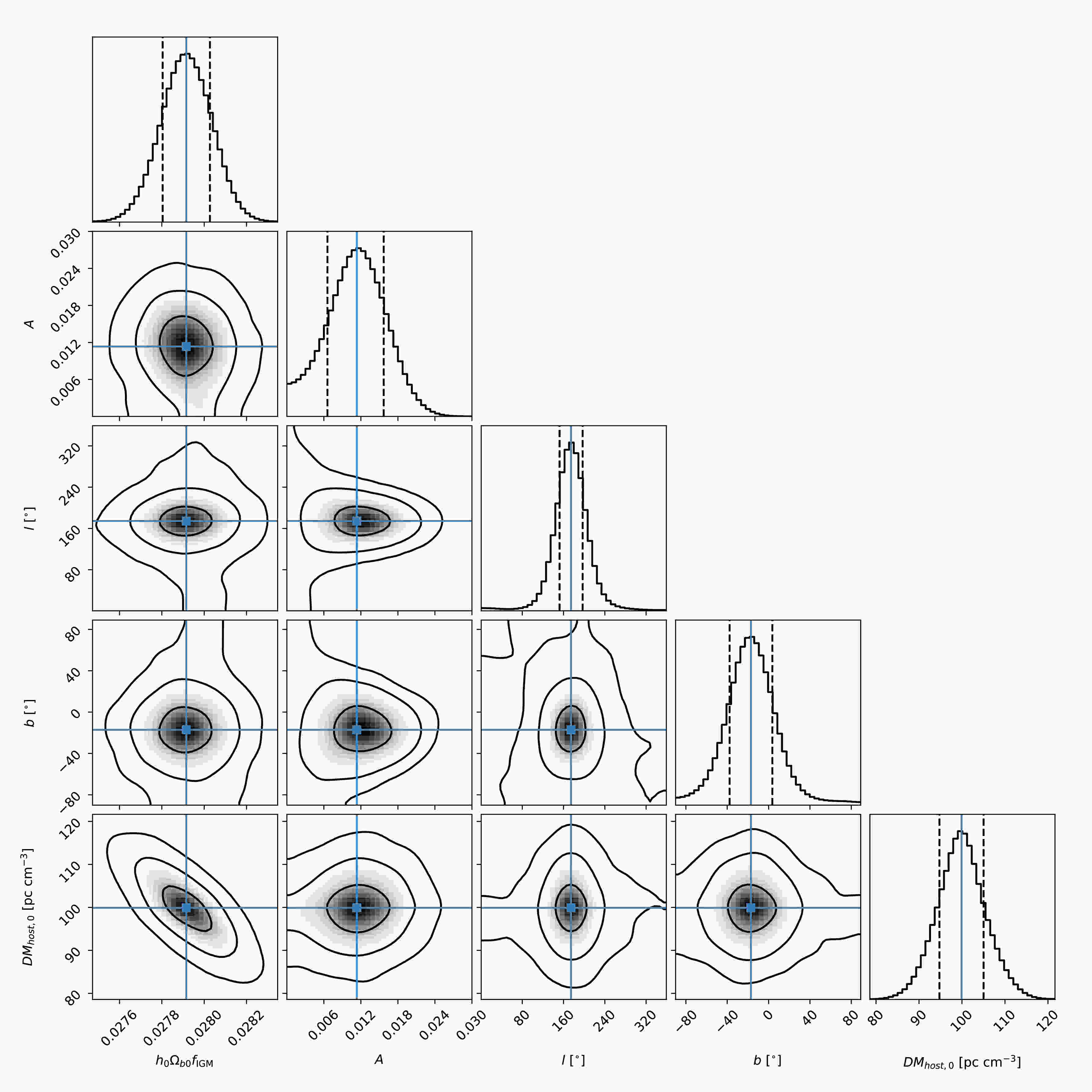
$ N = 100,200,300,...,1000 $ FRBs respectively, and then used the simulated data points to constrain the free parameters$ (h_0\Omega_{b0}f_{\rm IGM},A,l,b,{\rm DM_{host,0}}) $ . Figure 1 shows the posterior probability density functions and the 2-dimensional marginalized contours of the free parameters in one simulation for$ N = 800 $ , where the fiducial values of$ {\rm DM_{host,0}} $ and$ \sigma_{\rm host} $ are 100 and 20$ {\rm pc\; cm^{-3}} $ , respectively. It is shown that the parameters can be tightly constrained and the best-fit values are consistent with the fiducial values within$ 1\sigma $ uncertainty.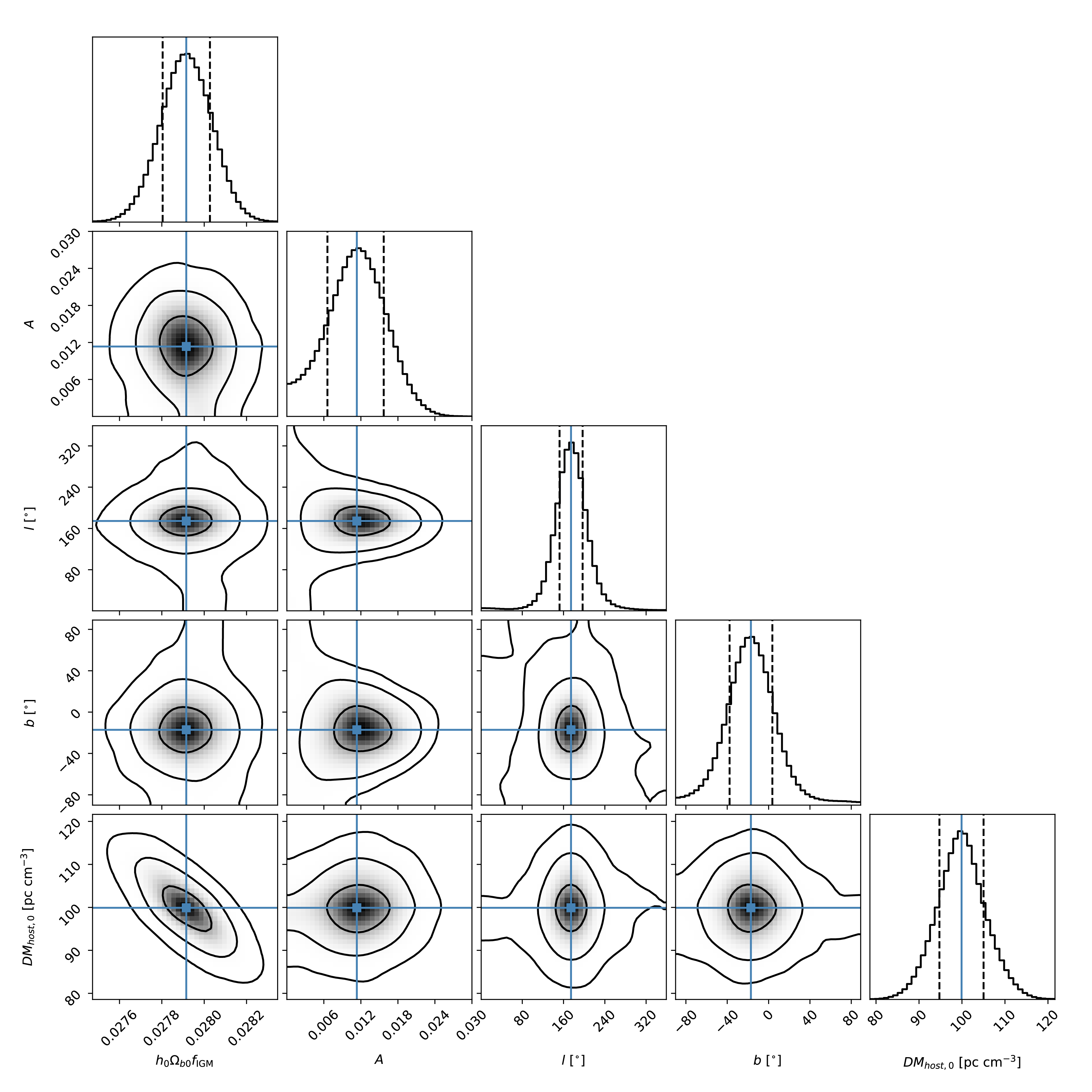
Figure 1. (color online) The best-fit results in a typical simulation with
$N = 800$ . The fiducial parameters are$A = 0.01$ ,${\rm DM_{host,0} = 100\;pc\; cm^{-3}}$ , and$\sigma_{\rm host,0} = 20\;{\rm pc\; cm^{-3}}$ . The blue solid and black dashed lines indicate the mean value and the$1\sigma$ uncertainty of the parameters, respectively.Owing to statistical fluctuation, the best-fit parameters differ in each simulation. Therefore, we simulated 1000 times for each N with different random seeds. Figure 2 shows the results for
$ N = 800 $ . The upper-left panel shows the best-fit dipole amplitudes and$ 1\sigma $ uncertainties in 1000 simulations. The red solid, red dashed, and red dotted lines represent the mean value, the fiducial value, and the zero value of the dipole amplitudes, respectively. The grey and blue error bars indicate that the dipole amplitudes are inconsistent and consistent with zero, respectively. We see that only 8 out of the 1000 dipole amplitudes are consistent with zero within$ 1\sigma $ ; hence there is a 99.2% probability that we can detect the anisotropic signal; that is,$ P(A>0) = $ 99.2%. The upper-right panel shows a histogram of the dipole amplitudes, which are well fitted by the Gaussian distribution, with a mean value$ \bar{A} = (1.14\pm0.01)\times 10^{-2} $ and a standard deviation$ \sigma_{A} = (0.36\pm0.01)\times 10^{-2} $ . The lower-left panel shows the best-fit dipole directions (black dots) in 1000 simulations. The central red plus at$ (180^{\circ},0^{\circ}) $ is the fiducial direction. The two black circles represent the circular regions of radius$ \Delta\theta < 20^{\circ} $ and$ \Delta\theta<40^{\circ} $ with respect to the fiducial direction, which encircle 3.0% and 11.7% of the whole sky, respectively. We find that 372 and 834 best-fit directions fall into the areas$ \Delta\theta<20^{\circ} $ and$ \Delta\theta<40^{\circ} $ , respectively; that is$ P(\Delta\theta<20^{\circ}) = $ 37.2% and$ P(\Delta\theta<40^{\circ}) = $ 83.4%. The lower-right panel shows the best-fit$ (h_0\Omega_{b0}f_{\rm IGM},{\rm DM}_{\rm host,0}) $ values, which are highly correlated.
Figure 2. (color online) The best-fit parameters in 1000 simulations with
$N = 800$ . The fiducial parameters are$A = 0.01$ ,${\rm DM_{host,0} = $ $ 100\;pc\; {\rm cm}^{-3}}$ , and$\sigma_{\rm host,0} = 20\;{\rm pc\; cm^{-3}}$ . Upper-left: the best-fit dipole amplitudes A with their$1\sigma$ uncertainty. The horizontal axis is the serial number of the simulation. The red solid, red dashed, and red dotted lines represent the mean value, the fiducial value, and the zero value of the dipole amplitudes, respectively. The grey and blue error bars indicate that the dipole amplitudes are inconsistent and consistent with zero, respectively. Upper-right: a histogram of the best-fit amplitudes. The black line is the best-fit result to a Gaussian distribution. Lower-left: the best-fit dipole directions$(l,b)$ . The central red plus at$(180^{\circ},0^{\circ})$ is the fiducial direction. The two black circles represent the circular regions of radius$\Delta\theta < 20^{\circ}$ and$\Delta\theta<40^{\circ}$ with respect to the fiducial direction, respectively. Lower-right: the best-fit$(h_0\Omega_{b0}f_{\rm IGM},{\rm DM}_{\rm host,0})$ values. The red plus is the fiducial value.We performed similar calculations for different values of N, and the results are shown in Table 1. From this table, we can see that as N increases, the probability that we can detect the anisotropy,
$ P(A>0) $ , also increases. At the same time, the probabilities$ P(\Delta\theta<20^{\circ}) $ and$ P(\Delta\theta<40^{\circ}) $ also increase. This tendency can be observed more clearly in the right panel of Figure 3, where we plot the probabilities as a function of N. For$ N\geqslant 200 $ , we can detect the anisotropic signal at more than a 90% confidence level. With about 400 (800) FRBs, the dipole amplitude can be constrained at a 95% (99%) confidence level; however, to correctly find the dipole direction, more FRBs are required. Even for$ N = 1000 $ ,$ P(\Delta\theta<20^{\circ}) $ is no more than 50%. To constrain the dipole direction within a$ 40^{\circ} $ uncertainty at an 80% confidence level, approximately 700 to 800 FRBs are necessary. Furthermore, from Table 1, we can see that as N increases, the mean value of the dipole amplitude$ \bar{A} $ becomes closer to the fiducial value. For$ N\geqslant 200 $ , the mean dipole amplitude$ \bar{A} $ is consistent with the fiducial value within$ 1\sigma $ uncertainty; see also the left panel of Figure 3, where we plot$ \bar{A} $ as a function of N.N $P(A>0)$ 

$P(\theta<20^{\circ})$ 

$P(\theta<40^{\circ})$ 

$A/10^{-2}$ 

$\sigma_A/10^{-2}$ 

100 0.862 0.093 0.329 1.86 0.86 200 0.904 0.141 0.449 1.51 0.67 300 0.933 0.198 0.567 1.34 0.53 400 0.953 0.234 0.638 1.25 0.50 500 0.968 0.272 0.685 1.19 0.44 600 0.979 0.293 0.744 1.17 0.41 700 0.985 0.355 0.794 1.17 0.39 800 0.992 0.372 0.834 1.14 0.36 900 0.996 0.388 0.854 1.12 0.34 1000 0.991 0.427 0.864 1.07 0.31 Table 1. The results of 1000 simulations for different values of N. The fiducial parameters are
$A = 0.01$ ,${\rm DM_{host,0} = 100\;pc\; cm^{-3}}$ , and$\sigma_{\rm host,0} = 20\;{\rm pc\; cm^{-3}}$ . First column: the number of FRBs in each simulation. Second column: the probability that we can detect a non-zero dipole amplitude. Third and fourth columns: the probabilities that the best-fit dipole direction is consistent with the fiducial direction within$20^{\circ}$ and$40^{\circ}$ , respectively. Fifth and sixth columns: the mean value and standard deviation of the dipole amplitudes, respectively.
Figure 3. (color online) Left: the mean value of the dipole amplitudes in 1000 simulations as a function of N. The error bar represents the standard deviation of the dipole amplitudes. Right: the probability that we can correctly reproduce the fiducial dipole amplitude or dipole direction as a function of N.
To investigate whether an increase in
$ \sigma_{\rm host} $ will affect our results, we set the fiducial values as$({\rm DM_{host,0}}, $ $ \sigma_{\rm host}) = (200,50)\; {\rm pc\; cm^{-3}}$ , and performed similar calculations. The results are compared with the case$({\rm DM_{host,0}},\sigma_{\rm host}) = (100,20)\; {\rm pc\; cm^{-3}}$ in Figure 3. The left panel plots the mean value of the dipole amplitudes in 1000 simulations as a function of N, and the right panel shows the probability that we can correctly reproduce the fiducial dipole amplitude or dipole direction as a function of N. We can see that the increase in$ \sigma_{\rm host} $ from 20 pc cm$ ^{-3} $ to 50 pc cm$ ^{-3} $ almost does not change the results. This can be understood from equation (10): the uncertainty on$ {\rm DM_{host}} $ is suppressed by a factor of$ 1/(1+z) $ due to cosmic dilation, and the total uncertainty is dominated by$ \sigma_{\rm IGM} $ , which we choose to be 100 pc cm$ ^{-3} $ in the simulation.To test if FRBs can probe a weaker anisotropic signal, we used a fiducial dipole amplitude
$ A = 0.001 $ and carried out similar calculations as before. Figure 4 shows the results of 1000 simulations, with$ N = 1000 $ FRBs in each simulation. The upper-left panel shows the best-fit dipole amplitudes. We found$ P(A>0) = $ 79.2%, meaning that there is still an$ \sim $ 80% probability that we can detect the anisotropic signal. However, the histogram of dipole amplitudes in the upper-right panel shows that the mean value and standard deviation of the dipole amplitudes is$ \bar{A} = (5.14\pm 0.10)\times 10^{-3} $ and$ \sigma_A = (2.40\pm 0.10)\times 10^{-3} $ , respectively. The mean dipole amplitude is approximately five times larger than the fiducial dipole amplitude, and it is inconsistent with the fiducial dipole amplitude within$ 1\sigma $ . Furthermore, the lower-left panel shows that the best-fitting dipole directions are randomly distributed in the sky,$ P(\theta<20^{\circ}) = $ 4.8% and$ P(\theta<40^{\circ}) = $ 14.6%, which means that we cannot correctly constrain the dipole anisotropy with 1000 FRBs if the dipole amplitude is in the region of 0.001.
Figure 4. (color online) The same as Figure 2, but with
$N = 1000$ and the fiducial dipole amplitude$A = 0.001$ . -
In this study, we investigated the use of FRBs to probe the possible anisotropic distribution of baryon matter in the Universe. We assumed that the distribution of baryon matter has a dipole form, and the fiducial dipole amplitude is chosen to be 0.01. According to simulations, 200 FRBs with a well-measured redshift and localization are sufficient to tightly constrain the anisotropy amplitude at a 90% confidence level. With 800 FRBs, the dipole amplitude can be constrained at a 99% confidence level. However, more FRBs are required to constrain the dipole direction. To constrain the dipole direction with uncertainty
$ \Delta\theta<40^{\circ} $ (which covers 11.7% of the sky) at an 80% confidence level, we require 700 to 800 FRBs; however, even 1000 FRBs are not sufficient to improve the confidence level to 90%. These results are not strongly affected by the uncertainty on the DM of the host galaxy; however, if the fiducial dipole amplitude is 0.001, 1000 FRBs are sufficient to correctly detect the anisotropic signal.In a recent study, Qiang et al. used FRBs to test the anisotropy of the Universe with a similar simulation method, but found a very different result [28]. They discovered that about
$ N = 2800 $ FRBs are required to find the cosmic dipole with an amplitude of 0.01, compared with$ N = 200 $ FRBs in our calculation. The difference may be due to several reasons. First, we used a different redshift distribution in the simulations; Qiang et al. assumed an exponential distribution$ P(z)\propto z\exp(-z) $ similar to that of gamma-ray bursts, while we assumed that the redshift distribution follows the SFR. Compared with the exponential distribution, the redshift distribution we used has more FRBs at high redshifts. Second, Qiang et al. directly assumed that${{\rm DM}_E}$ takes the dipole form, while we assumed that the baryon matter density$ \Omega_b $ takes the dipole form. In fact, the dipole of$ \Omega_b $ is equivalent to the dipole of$ {\rm DM_{IGM}} $ , since the latter is proportional to the former. However, it is not equivalent to the dipole of${{\rm DM}_E}$ , because$ {\rm DM_{\rm host}} $ is redshift-dependent and may be direction-dependent. Third, Qiang et al. used a six-parameter fit, which is one more parameter (the matter density$ \Omega_m $ ) than in our study. We fixed$ \Omega_m $ to the Planck value, which is equivalent to adopting the Planck value. Finally, Qiang et al. did not consider the statistical fluctuations. Their conclusion was based on one simulation for a given N, and, in some cases, a much smaller number of FRBs could still find the anisotropic signal.The progenitors of FRBs are still unclear. The most popular models evolve one or two compact objects (such as neutron stars and magnetars) in the center of an FRB source [1]. FRBs are expected to be frequent events in the Universe, although some of them cannot be observed due to low luminosity. Based on the compact binary merger model, the event rate of FRBs is estimated to be approximately
$(3-6) \times 10^4~ {\rm Gpc}^{-3}~ {\rm yr}^{-1}$ above the energy threshold$ E_{\rm th} = 3\times 10^{39} $ erg [58]. With the operation of new radio telescopes, such as the Australian Square Kilometre Array Pathfinder (ASKAP) [59], the Five-hundred-meter Aperture Spherical Telescope (FAST) [60], the Canadian Hydrogen Intensity Mapping Experiment (CHIME) [61], and the BAO from Integrated Neutral Gas Observations (BINGO) [62], more FRBs with well measured redshifts can be observed. We expected that the anisotropic signal of baryon matter will be detected or ruled out in the near future.
Probing the anisotropic distribution of baryon matter in the Universe using fast radio bursts
- Received Date: 2021-07-14
- Available Online: 2021-12-15
Abstract: We propose that fast radio bursts (FRBs) can be used as probes to constrain the possible anisotropic distribution of baryon matter in the Universe. Monte Carlo simulations show that 400 (800) FRBs are sufficient to detect the anisotropy at a 95% (99%) confidence level if the dipole amplitude has an order of magnitude of 0.01. However, more FRBs are required to tightly constrain the dipole direction. Even 1000 FRBs are insufficient to constrain the dipole direction within the angular uncertainty


 DownLoad: