Effect of dark energy models on the energy content of charged and rotating black holes

In General Relativity (GR), energy-momentum is a vital conserved quantity whose definition has been the subject of many investigations [1-6]. The definition of energy and momentum is a major dilemma in GR and unfortunately, there is still no generally accepted definition of energy and momentum. Generally, a spacetime shall not be stationary (and particularly shall not be static) and hence the energy conservation may be lost. Due to this fact there is a long-standing problem of the definition of energy (mass) in GR [7]. If the spacetime is a static spacetime, then a timelike isometry or Killing Vector (KV) exists and the energy of a test particle can easily be defined. However, in the absence of a timelike isometry the test particle's energy is not defined and hence the energy in the gravitational field is not well defined. For gravitational wave spacetimes, the problem of defining the energy content is particularly severe [8].

Different notions of approximate symmetries have been utilized to resolve the problem of energy conservation in GR [9]. The idea of approximate or broken Lie symmetries arises from the grouping of Lie theory and perturbation theory. Hence, two different approximate symmetry theories have been introduced using this idea. The first theory was presented by Baikov, Gazizov and Ibragimov (BGI) [10] while the second was introduced by Fushchich and Shtelen [11]. Here in this article we will follow the notion of approximate symmetries given by BGI.

In 4D spacetime, the no-hair theorem depicts that all black hole (BH) solutions to the Einstein–Maxwell field equations are particularly characterized by three parameters: mass M, electric charge Q, and angular momentum J. The spacetime characterized by these three parameters is known as the charged-Kerr (CK) spacetime. In the spherically symmetric and static case, where the parameter J disappears, we get the Reissner-Nordstrom (RN) spacetime, and further if charge Q goes to zero we get the Schwarzschild spacetime [12]. The charged spinning solution, or CK metric [13], is the spinning generalization of RN and the electrically charged version of the Kerr metric.

In the last few years, cosmological observations found that the Universe is going through a period of accelerating expansion which demands the presence of some unidentified form of energy recognized as DE [14]. The current measurements of cosmic microwave background anisotropy by PLANCK also verified this result [15]. The two famous candidates for this DE are the cosmological constant and quintessence [16].

The Universe accelerating expansion demands the equation of state (EOS) parameter $ (\omega = p/\rho) $ to be in the range $ -1 <\omega < -{1}/{3} $. The cosmological constant is defined by a fixed value of EOS parameter $ {\omega}_{c} = -1 $, whereas quintessence is defined as a dynamical, time evolving, spatially inhomogeneous component with negative pressure. For the quintessence DE model, the EOS parameter $ {\omega}_{q} \in \left(-1,-{1}/{3}\right) $ [17]. Unlike the cosmological constant, the quintessential pressure and energy density evolve in time, and ω may also do so. Other forms of DE include chameleon fields [18], K-essence [19], a tachyon field [20], phantom DE [21], dilaton DE [22] and a frustrated network of domain walls and cosmic strings [23]. The frustrated network of cosmic strings has the EOS $ {\omega}_{n} = -{1}/{3} $, and for this particular value of the state parameter the Universe remains unchanged (neither accelerates nor decelerates) [24-27].

The Minkowski metric being maximally symmetric gives conservation laws for energy, momentum, spin angular momentum and linear momentum. If one moves from flat to non-flat spacetime, a few of the conservation laws do not show up because of the existence of the strong gravitational field. These missing conservation laws were first recouped by Kara et al. using approximate Lie symmetry methods for differential equations [28]. They recovered all the lost conservation laws for the Schwarzschild BH. The same approach of approximate Lie symmetries was used to recover the missing conservation laws for RN [29], RN with quintessence [30, 31], Kerr-Newmann (KN) [32], KN anti-de Sitter [33], Bañados-Teitelboim-Zanelli (BTZ) [34], slowly-rotating Horava-Lifshitz [35], Bardeen [36] spacetimes and gravitational wave spacetimes [8].

The spacetime solution for the spherically symmetric charged BH surrounded by a quintessence field has been discussed by Kiselev [37]. This solution reduces to the RN BH solution in the the absence of the quintessence field. The gravitational energy (mass) of the quintessential RN BH has been thoroughly discussed in previous studies [30, 31]. These obtained an explicit relation of the energy content which is dependent on the square of the charge-to-mass ratio $ {Q^2}/{M^2} $, DE parameter α and the radial distance r. The energy content of CK spacetime has also been studied comprehensively [32]. The energy scale factor of the CK BH spacetime found depends on the spin parameter a and square of the charge-to-mass ratio $ {Q^2}/{M^2} $ of the BH, which correlates the electromagnetic self-energy with the gravitational self-energy. In the current paper, we will explore the energy content of the CK BH surrounded by DE using approximate Lie symmetries, for different values of EOS parameter ω. We will consider the border cases of quintessence DE i.e. $ {\omega}_{c} = -1 $ and ${\omega}_{n} = -{1}/{3}$. The energy content of the CK BH surrounded by DE will be investigated at an intermediate value of the quintessence DE, i.e. at ${\omega}_{q} = -{2}/{3}$. Specifically, we will discuss the effects of DE models on the energy content of the CK spacetime surrounded by DE. For this purpose, we take the mass, charge, and spin of the BH in terms of perturbation parameter ϵ, and construct the perturbed geodesic equations of the second order. Here we retain the first and second powers of ϵ, neglecting its higher powers. More specifically, in the set of determining equations for perturbed geodesic equations of second order, the coefficient of $ \dfrac{\partial}{\partial{s}} $ (in the symmetry generator given in Section II) collects a rescaling factor (given in Section III). Since energy conservation is associated with time-translational symmetry and s is the proper time, therefore the energy in the CK spacetime surrounded by DE rescales by some factor [discussed in Section III]. We also give a comparison of the scaling factor obtained here with the expressions already obtained in the literature for the energy of the CK spacetime without DE [32]. It is observed that at all three values of ω, the energy content of the CK BH surrounded by DE decreases due to the presence of the DE. This is discussed in detail in the following sections.

In the next section, we briefly review the definitions to be used in this work. In Section III we discuss different cases to examine the approximate Lie symmetries of the perturbed geodesic equations for the CK metric surrounded by DE. The influence of DE on the energy content of the charged-Kerr spacetime surrounded by DE is discussed in the same section. In Section IV we present our summary and discussion.

A vector field defined on a real parameter fibre bundle over the manifold [38]

is professed to be an approximate Lie symmetry generator of 2nd order for a perturbed system of 2nd-order geodesic equations

if the following condition holds

where,

$ \Xi = \Xi_{0}+\epsilon{\Xi_{1}}+{\epsilon}^2{\Xi}_{2} $, $ {\chi}^{\alpha} = {\chi}^{\alpha}_{0}+\epsilon{{\chi}^{\alpha}}_{1}+{\epsilon}^2{{\chi}^{\alpha}}_{2} $ and $ \alpha,\upsilon = $$ 0,1,2,3 $ respectively.

For the vector fields $ {\bf{W}}_{0},{\bf{W}}_{1} $ and $ {\bf{W}}_{2} $, we take the second prolongation because we are interested in finding the approximate Lie symmetries of the 2nd order for the 2nd-order perturbed differential equations. The second prolongation for W is given by:

The vector fields $ {\bf{W}}_{i} $ $ (i = 0,1,2) $ given in equation (1) depict the exact, 1st-order and 2nd-order approximate parts of the symmetry generator W. The term $ {\bf{Y}}_{0} $ represents the exact part of the equation while the terms $ {\bf{Y}}_{1} $ and $ {\bf{Y}}_{2} $, given in equation (2), are the approximate parts of the system of perturbed geodesic equations. The generators $ {\bf{W}}_{i} $ $ (i = 1,2) $ are called the non-trivial symmetry generators if the symmetry generator $ {\bf{W}} = {\bf{W}}_{0}+{\epsilon}{\bf{W}}_{1}+ $$ {\epsilon}^2{\bf{W}}_{2} $ exists with $ {\bf{W}}_{0}\ne0 $ or $ {\bf{W}}_{1}\ne0 $ and $ {\bf{W}}_{2}\ne k{\bf{W}}_{0} $, $ {\bf{W}}_{2}\ne k{\bf{W}}_{1} $, (k is some arbitrary number). By applying the approximate symmetry condition given in equation (3) to the perturbed system of 2nd-order geodesic equations, we will obtain a significant result of the energy rescaling factor (explained in Section III).

The vector field W is said to be a Noether symmetry generator for the Lagrangian $ L(s,{x}^{\upsilon},\dot{x}^{\upsilon}) $, if the following condition holds:

where $ h(s,{x}^{\upsilon}) $ is the gauge function and the total derivative operator D is given by:

The Noether theorem that reveals the importance of the Noether symmetries is stated below [39].

Theorem. If W is a Noether symmetry generator corresponding to a Lagrangian $ L(s,{x}^{\upsilon},\dot{x}^{\upsilon}) $ of the Euler-Lagrange equations of motion, then I in equation (8) is a constant of motion associated with the symmetry generator W.

(We use this result in Section III, to calculate the exact first integrals).

The 4D CK spacetime generated by an axially symmetric gravitational source of mass M, charge Q, and spin a, surrounded by quintessence DE with EOS parameter $ {\omega_q} $, is described by the following metric [40]

where

In the above equation (10), α is the quintessence parameter, which depicts the magnitude of the quintessence scalar field around a BH, satisfying the following inequality [40]:

The horizons can be calculated by substituting $ \Delta_{r} = 0 $.

The inequality given in (11) holds when the cosmological horizon determined by the quintessential DE exists. It is observed that the total charge Q does not affect the range of α, i.e. the range of α remains the same in the absence of the charge Q [40]. When quintessence does not exist, i.e. as $ \alpha\to 0 $, the metric given in (9) reduces to the KN BH, which further reduces to the rotational situation in the Kiselev quintessence BH, i.e. the Kerr BH as $ Q\to 0 $. In the particular case when $ a\to 0 $, the metric given in (9) corresponds to the RN spacetime surrounded by quintessence DE, and in the absence of the total charge Q it further reduces to the quintessential Schwarzschild BH according to the Kiselev description. In the present paper, we consider three different DE models, i.e. $ {\omega}_{c} = -1 $, ${\omega}_{q} = -{2}/{3}$ and ${\omega}_{n} = -{1}/{3}$, to discuss the gravitational energy (mass) and 2nd-order approximate Lie symmetries of CK spacetime surrounded by DE.

In the cosmological constant model, we consider $ {\omega}_{c} = -1 $ and from (11), $\alpha \leqslant {1}/{16}$. In this particular case the function $ \Delta_{r} $ is defined as

To explore the approximate Lie symmetries of the CK BH surrounded by the DE with $ {\omega}_{c} = -1 $, we define the mass M, charge Q and spin parameter a of the BH as a small perturbation parameter ϵ. Therefore, we consider

To avoid a naked singularity, $0 < k_1+k_2 \leqslant {1}/{4}$. Using (13) in the above metric (12) and retaining the first and second powers of ϵ, we construct the following system of perturbed 2nd-order geodesic equations:

In the absence of the DE parameter, i.e. when $ \alpha \to 0 $, the system of 2nd-order perturbed geodesic equations $(14)-(17)$ reduces to the system of a CK BH [32]. For $ k_{2} = 0 $, the above system of equations $(14)-(17)$ represents the system of perturbed geodesic equations for the quintessential RN spacetime [30, 31]; in the absence of DE parameter α, we get the perturbed system for RN spacetime [29]; and as the electric charge $ Q \to 0 $ we get the perturbed system for the Schwarzschild spacetime [28]. Now we calculate the 2nd-order approximate Lie symmetries for the above equations $(14)-(17)$. For this purpose we examine the exact and 1st-order approximate Lie symmetries first, by applying the approximate symmetry condition (3) in the above equations. Therefore, by substituting $ \epsilon = 0,{\epsilon}^2 = 0 $, we obtain a system of exact (unperturbed) geodesic equations. Using Maple software we get the following six exact Lie symmetries.

The exact Lie symmetries $ {\bf{Y}}_{0} $ and $ {\bf{Y}}_{1} $, corresponding to $ \Xi = {g}_{0}{s}+{g}_{1} $, give the dilation algebra $ d_2 $. The exact Lie symmetry generator $ {\bf{Y}}_{1} = \partial/\partial{s} $ represents the time-translational symmetry as s is the proper time, and the other four symmetry generators $ {\bf{Y}}_{2} $, $ {\bf{Y}}_{3} $, $ {\bf{Y}}_{4} $ and $ {\bf{Y}}_{5} $, which form the symmetry algebra $ so(3)\oplus{\mathbb{R}} $ correspond to energy and momentum conservation.

To explore the 1st-order approximate symmetries, we take $ {\epsilon}^2 = 0 $, in the above system $(14)-(17)$. Now, by applying the approximate symmetry condition given in equation (3) and the exact (unperturbed) Lie symmetries given in equation (18), we obtain a set of 70 partial differential equations (PDEs), keeping only first terms of ϵ. After solving this set of determining equations we obtain the six approximate Lie symmetry generators (trivial) of 1st-order given in (18). Next we use these exact and the 1st-order approximate symmetries to calculate the approximate Lie symmetries of order two for the above system of equations $(14)-(17)$. Using the approximate symmetry condition given in equation (3), and retaining terms with $ {\epsilon}^2 $, we obtain a system of 70 PDEs once again. Consequently, we do not find any new symmetry generators, and recoup the same six Lie symmetries given in (18) as approximate trivial symmetry generators of the 2nd order. It is found that in the set of 70 PDEs for the 1st-order approximate symmetry case, the terms that contain $ \Xi_{s} = g_{0} $ disappear. But in the case of approximate Lie symmetries of order two for the CK BH surrounded by DE, $ \Xi_{s} = g_{0} $ do not vanish instinctively, but collect a rescaling factor to vanish, in order to satisfy the PDEs. In this case we find the following energy rescaling factor:

Next we consider the extreme effects on the energy, in the equatorial plane, i.e. in the regions where the rotational effect is maximam ($\theta = {\pi}/{2}$), which implies $ \dot{\theta} = 0 $.

The scaling factor contains the derivatives of t and ϕ, and the derivatives only apply to the paths of the particles. Hence, to get the energy of the underlying spacetime, we replace the derivatives by the exact first integrals (obtained by using Neother theorem, i.e. $\dot{t} = \dfrac{M}{1-\alpha{r}^2}, $$ \dot{\phi} = -\dfrac{M^2}{2r^2}$) and using (13) in (19) we get the energy rescaling factor for the CK spacetime surrounded by DE with $ {\omega}_{c} = -{1} $, as a function of charge, gravitational mass, spin parameter of BH along with DE parameter.

As $ {\alpha\to 0} $, we get the energy rescaling factor for the CK metric without DE [32]:

It should be noted, if we retain only first powers of α in the expansion of (20), the terms involving charge Q get canceled. Therefore, to include the effect of charge along with spin and the DE, we retained the first and second powers of α in the expansion of (20), to separate the terms involving α from those which are independent of the parameter α. We get the following energy rescaling factor:

From equations (21) and (22), we observe that the total energy in the CK spacetime surrounded by DE is different from the total energy in the CK BH by the given expression:

In equation (23), the parameters of the BH, charge Q, spin a and the DE parameter α appear at the same order. Also, we observe that the presence of the cosmological constant term will increase or decrease the total energy of the underlying spacetime if the behavior of the expression (23) is positive or negative. The investigation of the behavior of $ {E}_{{c}} $ is explained in the subsequent figures.

From the graphical results (Fig. 1, Fig. 2, Fig. 3) we observe that the behavior of $ {E}_{c} $ is decreasing. Therefore, we remark that the contribution of cosmological constant does not play any role in increasing the energy content of the CK metric surrounded by the DE despite considering the different values of charge Q, spin parameter a and DE parameter α. Hence, in the cosmological constant model with $ {\omega}_{c} = -1 $, the influence of DE results in reducing the total energy (mass) of the CK spacetime surrounded by the DE.

Figure 1.  (color online) Plots showing the behavior of $ {E}_{c} $ for the CK BH surrounded by DE for $ {\omega}_{c} = -1 $ with different values of α and fixed values $ Q = 0.89 $, $ M = 1 $, $ a = 0.5 $.

Figure 2.  (color online) Plots showing the behavior of $ {E}_{c} $ for the CK BH surrounded by DE for $ {\omega}_{c} = -1 $ with different values of a, $\alpha \leqslant {1}/{16}$ and fixed values $ Q = 0.89 $, $ M = 1 $ and $ r = 17 $.

Figure 3.  (color online) Plots showing the behavior of $ {E}_{c} $ for the CK BH surrounded by DE for $ {\omega}_{c} = -1 $ with different values of Q, $\alpha \leqslant {1}/{16}$ and fixed values $ a = 0.5 $, $ M = 1 $, and $ r = 3.5 $.

In the quintessence DE model, we consider a fixed value of the EOS parameter ${\omega}_{q} = -{2}/{3}$, and for this particular value the function $ \Delta_{r} $ takes the following form

From equation (11), we see that for ${\omega}_{q} = -{2}/{3}$, $\alpha \leqslant {1}/{6}$. Using (13) in the above metric and preserving only first and second powers of ϵ, we construct a system of 2nd-order perturbed geodesic equations given below:

When the quintessence does not exist, i.e. as $ \alpha \to 0 $, the above system of equations $(25)-(28)$ corresponds to the perturbed system for the KN spacetime [32]. As in the prior case, we study the 2nd-order approximate Lie symmetries for this BH spacetime and recovered the same six Lie symmetry generators given in (18) as trivial 2nd-order approximate Lie symmetries.

The exact symmetry generators and the trivial 1st-order approximate symmetry generators did not give any new result, but in the 2nd-order approximate symmetries of the CK BH surrounded by DE we noticed the terms containing $ \Xi_{s} = g_{0} $ pick up a rescaling factor which consists of terms involving $ \dot{t} $, $ \dot{\phi} $ and $ \dot{\theta} $, to provide a necessary cancellation. We consider the equatorial plane, i.e. $\theta = {\pi}/{2}$, which implies $ \dot{\theta} = 0 $. This rescaling factor corresponds to the rescaling of the energy in the spacetime field of the CK BH with quintessence. Hence, for the quintessence DE model we find the following rescaling factor:

After replacing the derivatives by the exact first integrals, i.e. $ \dot{t} = \dfrac{M}{1-\alpha{r}}, \dot{\phi} = -\dfrac{M^2}{2{r^2}} $, we get:

Using (13) in (30) we get the rescaling factor of energy for the CK spacetime surrounded by DE that is dependent on charge Q, gravitational mass M and spin a of BH along with quintessence parameter α:

In the absence of quintessence parameter α we get the energy rescaling factor for CK spacetime [32].

Now we check the influence of quintessence DE on the total energy of underlying spacetime. In the expansion of above equation (31), retaining terms with α and neglecting all higher powers of α we get the following expression:

From equation (32), it is clear that the energy in the CK BH surrounded by the quintessence differs from the energy in the CK BH [32] by the expression given below:

In equation (33), charge Q and spin a appear quadratically while the DE parameter α comes in linearly. It is noted that the effect of quintessence DE may increase or decrease the energy content of the underlying spacetime if the function $ {E}_{q} $ is increasing or decreasing. The effect of quintessence on the energy content of the CK BH surrounded by quintessence is explained through the graphs below.

From Fig. 4, Fig. 5 and Fig. 6, we observe that the behavior of the function $ {E}_{q} $ is decreasing, which shows that the energy of the underlying spacetime may decrease for different values of spin parameter a, charge Q and quintessence parameter $\alpha \leqslant {1}/{6}$. Hence, for ${\omega}_{q} = -{2}/{3}$, the increase in the energy content is improbable, despite considering different values of BH parameters and the DE parameter.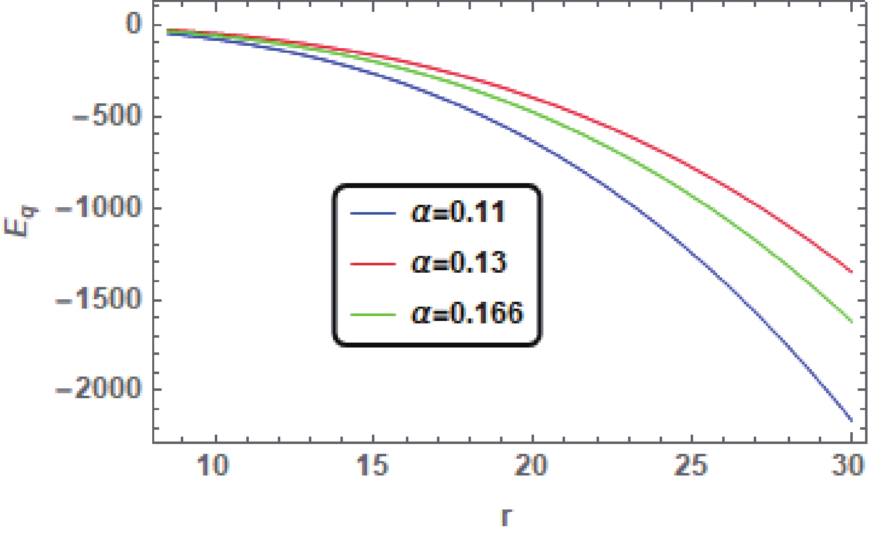

Figure 4.  (color online) Plots showing the behavior of $ {E}_{q} $ for the CK BH surrounded by quintessence for ${\omega}_{q} = -{2}/{3}$ with different values of α and fixed values $ Q = 1 $, $ M = 1 $, $ a = 0.5 $.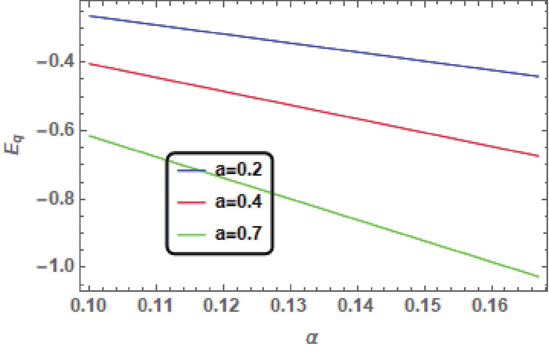

Figure 5.  (color online) Plots showing the behavior of $ {E}_{q} $ for the CK BH surrounded by quintessence for $ {\omega}_{q} = -{2}/{3} $ with different values of a, $ \alpha \leqslant {1}/{6}$ and fixed values $ Q = 0.89 $, $ M = 1 $, and $ r = 15 $.

Figure 6.  (color online) Plots showing the behavior of $ {E}_{q} $ for the CK BH surrounded by quintessence for $ {\omega}_{q} = - {2}/{3} $ with different values of Q, $ \alpha \leqslant {1}/{6} $ and fixed values $ a = 0.5 $, $ M = 1 $ and $ r = 0.9 $.

It is well known that the frustrated network of cosmic strings may produce negative pressure for ${\omega}_{n} = -{1}/{3}$ [24]. With ${\omega}_{n} = -{1}/{3}$, the function $ \Delta_{r} $ is defined as:

Like the previous two cases, here we also construct the system of 2nd-order perturbed geodesic equations by introducing the BH parameters in terms of a perturbation parameter. The perturbed geodesic equations of 2nd-order with ${\omega}_{n} = -{1}/{3}$ are given below:

For $\omega{_n} = -{1}/{3}$, $ 0<\alpha<1/2 $. The above system of approximate equations $(35)-(38)$ reduces to the system of the CK BH [32] when the DE does not exist ($ \alpha\to 0 $).

First, we illustrate the exact symmetries for the above system of perturbed differential equations $(35)-(38)$. For the exact case we substitute $ \epsilon = 0, \epsilon^2 = 0 $ (no mass, charge and spin) in the above equations and get an exact system of geodesic equations. Using the approximate symmetry condition given in equation (3) in the unperturbed system we get the eight Lie symmetry generators. Out of these eight symmetries, six Lie symmetries are given in (18) and the remaining two symmetries are: $ {\bf{Y}}_{6} = t\partial/\partial{t} $ and $ {\bf{Y}}_{7} = r\partial/\partial{r} $. Now letting $ \epsilon^2 = 0 $ (no charge and spin) we get the 1st-order approximate geodesic equations. Next, we calculate the 1st-order approximate symmetries, using the approximate symmetry condition given in (3) and the exact (unperturbed) Lie symmetry generators. At this stage we find a set of 70 PDEs. After solving this system of equations we obtain the same eight symmetries as 1st-order trivial approximate symmetries. Using these exact and 1st-order approximate symmetries into the equations $(35)-(38)$, we obtain the trivial approximate Lie symmetry generators of second order. Hence, we conclude that for the EOS parameter ${\omega}_{n} = -{1}/{3}$, no non-trivial symmetry is obtained at first and second order like the earlier cases discussed here. In this calculation it is noticed that in the set of 70 PDEs, for the case of 2nd-order approximate Lie symmetries the terms involving $ \Xi_{s} = g_{0} $ do not disappear automatically but, pick up a scale factor (energy rescaling factor) to make the system of equations (PDEs) consistent. The scale factor has derivatives of t, ϕ and θ. We consider the equatorial plane, i.e. when $\theta = {\pi}/{2}$, and get the following scale factor:

Now we replace these derivatives ($ \dot{t} $ and $ \dot{\phi} $) by the exact first integrals of the geodesic equations. Using equation (8) and the exact Lie symmetry generators we get $ \dot{t} = \dfrac{M}{1-\alpha}, \dot{\phi} = -\dfrac{M^2}{2{r^2}} $. Hence, in the case of ${\omega}_{c} = -{1}/{3}$, we get the following rescaling factor of energy for the CK BH spacetime surrounded by DE

In the absence of DE we get the energy rescaling factor for the CK BH [32] from (40). Now we discuss the influence of DE on the energy content of the quintessential CK BH. It is observed, for ${\omega}_{n} = -{1}/{3}$, the total energy in the CK BH surrounded by DE varies from the energy in CK BH by the following expression (details are given in Appendix):

Unlike the previous cases, here the contribution due to the DE term $ {E}_{n} $ is independent of the charge Q. In order to analyze the significant features of DE, we sketch the expression (41) versus DE parameter α and radial distance r and examine its dependence on the BH parameters M and a.

From Fig. 7, it is clear that the behavior of $ {E}_n $ is decreasing for different values of the DE parameter α. Fig. 8 shows the effect of the DE with different values of spin a. Here we observe that if the DE parameter α is initially small, then the value of $ {E}_n $ will increase at first and then it shows a gradual decline for the larger values of α. Hence, here we remark that the contribution of the DE term for ${\omega}_{n} = -{1}/{3}$, first results in increasing the total energy of the underlying spacetime for very small α, and then decreasing for comparatively larger values of α.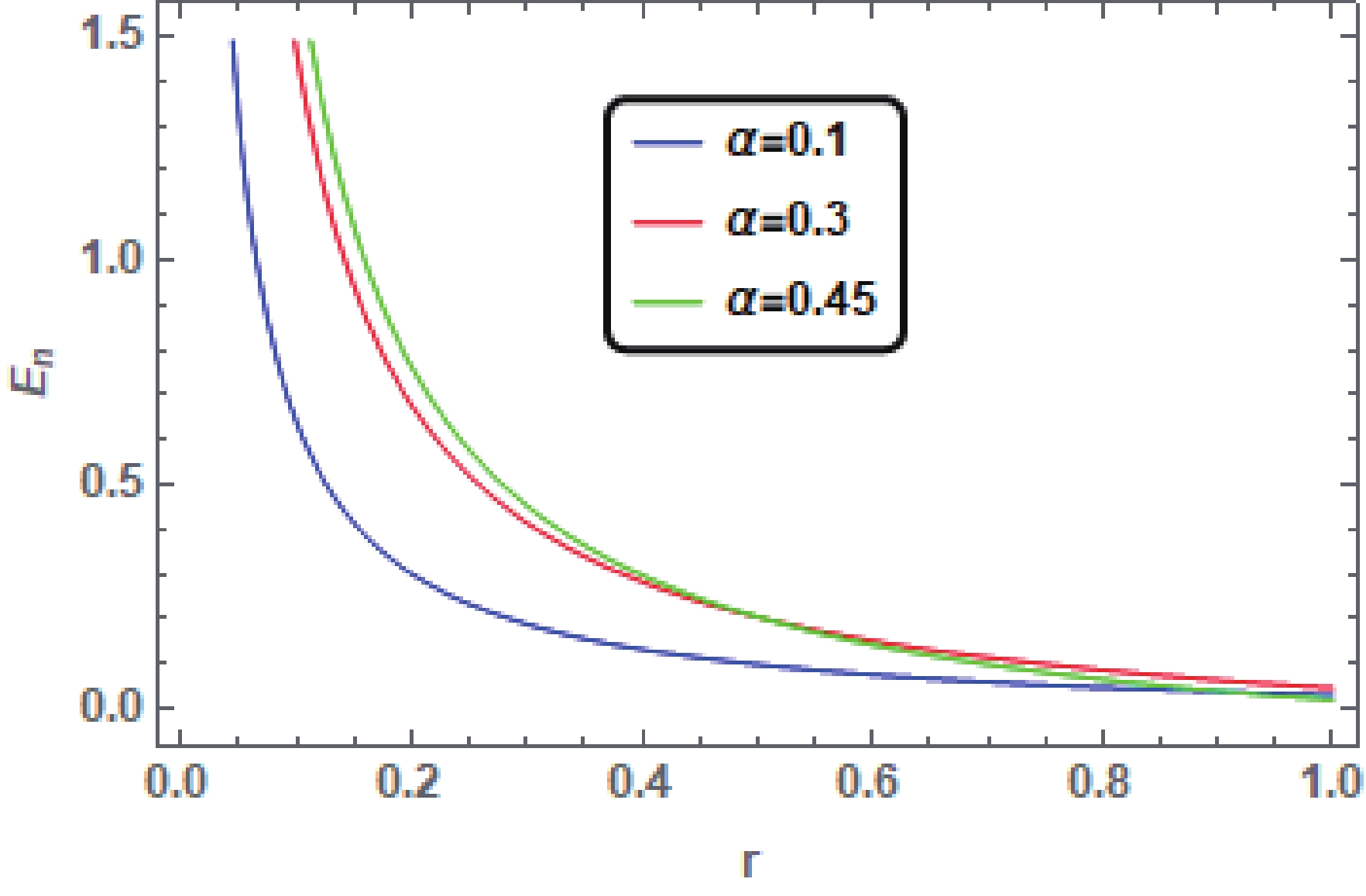

Figure 7.  (color online) Plots showing the behavior of $ {E}_n $ for the CK BH surrounded by DE for $ {\omega}_{n} = - {1}/{3} $ with different values of α and fixed values $ M = 1 $, $ a = 0.7 $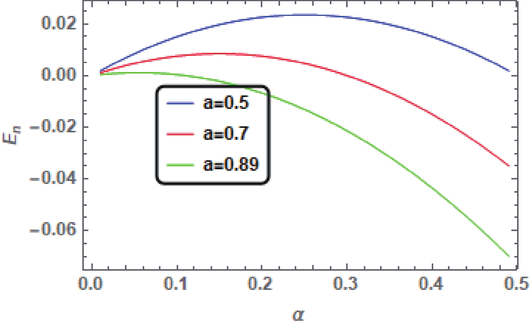

Figure 8.  (color online) Plots showing the behavior of $ {E}_n $ for the CK BH surrounded by DE for $ {\omega}_{n} = - {1}/{3} $ with different values of a, $ 0<\alpha<1/2 $ and fixed values $ M = 1 $ and $ r = 2 $.

To examine the energy content of the charged and rotating BHs surrounded by DE, 2nd-order approximate Lie symmetries have been studied intensively. For this purpose, we have introduced the parameters of BH in terms of a small perturbation parameter ϵ and constructed a system of 2nd-order perturbed geodesic equations by retaining terms up to $ \epsilon^2 $ only. We have considered three different DE models to study the gravitational energy and approximate Lie symmetries of the CK spacetime surrounded by DE:$ (i) $ cosmological constant model with $ {\omega}_{c} = -1 $, $ (ii) $ quintessence DE model with ${\omega}_{q} = -{2}/{3}$, $ (iii) $ frustrated network of cosmic strings with ${\omega}_{n} = -{1}/{3}$. Initially, we investigated the exact symmetries (no mass, charge and spin), and for $ {\omega}_{c} = -{1} $ and ${\omega}_{q} = -{2}/{3}$ we have obtained six symmetries which form a six dimensional Lie algebra $ so(3)\oplus{\mathbb{R}}\oplus{d_{2}} $, given in (18). For ${\omega}_{n} = -{1}/{3}$, we obtained two more Lie symmetries $ {\bf{Y}}_{6} = t\partial/\partial{t} $ and $ {\bf{Y}}_{7} = r\partial/\partial{r} $. Using the exact symmetries we have found the approximate Lie symmetries of first order (no charge and spin) and obtained the same exact Lie symmetries as trivial 1st-order approximate symmetries. In the set of 70 PDEs for the 1st-order approximate symmetry case, the terms that contain $ \Xi_{s} = g_{0} $ have disappeared and do not collect any energy rescaling factor, and we have only recovered the lost conservation laws as 1st-order approximate conservation laws. Therefore, since we were interested in finding the energy content of the CK BHs, we have studied the approximate Lie symmetries of second order, using exact and 1st-order approximate symmetries. Again we get no non-trivial approximate symmetry generator at 2nd order. It has been observed that in the case of approximate Lie symmetries of second order for the CK BH surrounded by DE, $ \Xi_{s} = g_{0} $ do not vanish instinctively and collect a rescaling factor to vanish, in order to satisfy the determining equations. In spite of the fact that there are no non-trivial 2nd-order approximate Lie symmetries, we have obtained the non-trivial result of energy rescaling from the application of 2nd-order approximate Lie symmetries in all the three cases we have discussed here.

As for different BH spacetimes [29-36] and gravitational waves [8] discussed in the literature, we have obtained the scaling factors for the CK spacetime with DE for the three different values of ω. It is observed that in all three cases of the CK BH with DE the energy rescaling factors contain the derivatives of t, θ and ϕ. We have considered the extreme effects on the energy, i.e. $\theta = {\pi}/{2}$, which gives $ \dot{\theta} = 0 $, and replaced the remaining derivatives $ \dot{t} $ and $ \dot{\phi} $ by the exact first integrals of geodesic equations, and obtained the energy rescaling factors in terms of charge, mass, spin, radial distance and DE parameter given in equations $ (20), (31) $ and (40). In all three cases the spin of the BH does not appear explicitly and only appears in a product with the DE parameter α. As the DE parameter $ \alpha\to{0} $ the energy rescaling factor of the CK BH can be recouped [32].

The effect of DE on the energy content of the CK BH surrounded by DE is spotted through graphical analysis. It is found that in all the three cases the effect of the DE results in reducing the energy content of the CK BH surrounded by DE, despite taking the different values of the charge Q, spin a and the DE parameter α. In equation (23), from the first term we have observed that the contribution of energy due to the charge, i.e. the electromagnetic energy, and the energy extracted by rotation add up and the term which is independent of Q and a and dependent on DE parameter α gets subtracted from it. This implies that the pure DE term is dominating and hence causing the decrease in the total energy of the underlying spacetime with $ {\omega}_{c} = -1 $, as evident from Fig. 1, Fig. 2 and Fig. 3. From expression (33), we can see that the contribution in energy $ E_{q} $ due to the charge and rotation is multiplied by the DE parameter α. The terms involving rotation a get subtracted from the term that is dependent on charge Q and the graphical results show that the total behavior of the energy is decreasing in the case of $ \omega_{q} = -2/3 $. This implies that the terms involving rotation dominate the term which involves the charge parameter Q.

The effect of the DE models on the energy content of the RN BH surrounded by DE with $ {\omega}_{c} = -1 $, ${\omega}_{q} = -{2}/{3}, $$ -{1}/{2}$ and ${\omega}_{n} = -{1}/{3}$ has been thoroughly discussed in the literature [30, 31]. For $ {\omega}_{c} = -1 $ and ${\omega}_{q} = -{2}/{3}, -{1}/{2}$, the effect of the DE gives the similar findings, i.e. the influence of the DE may result in decreasing the total energy content of the RN BH surrounded by DE for different values of the BH parameters and the DE parameter. In the case of the RN BH [30], for ${\omega}_{n} = -{1}/{3}$, it was observed that the contribution of DE to the total energy content of the spacetime, involved the square of the charge-to-mass ratio $ {Q^2}/{M^2} $ of the BH, which correlates the electromagnetic self-energy with the gravitational self energy, was added in and hence resulted in increasing the energy content of the underlying spacetime. Here in the case of the CK spacetime surrounded by DE with ${\omega}_{n} = -{1}/{3}$, it is noticed that the contribution to the energy due to the presence of the DE is independent of charge Q and depends on spin a and mass M of the BH, radial distance r and DE parameter α, as given by (41). Furthermore, from (41) it can be seen that the term involving rotation is to be subtracted from the term that depends on the DE parameter α. Since the energy extracted by rotation from the spacetime is subtracted from the total energy of the spacetime, it hence may be the cause of decrease in the energy content of the CK spacetime surrounded by DE. The presence of DE causing the reduction in the energy content of the CK BHs encircled by DE favours the idea of mass (energy) reduction of BHs by the accretion of DE onto BHs given by Babichev et al. [41]. Also, at ${\omega}_{n} = -{1}/{3}$ we have noticed from Fig. 8 that the energy $ E_{c} $ due to the presence of the DE parameter α first increases and then decreases for different values of spin parameter a. It is known that at this value of EOS parameter the Universe remains static [24], and this may be correlated with our result of first increasing and then decreasing the energy $ E_{c} $, as shown in Fig. 8, i.e. the increasing and the decreasing behavior may balance each other and as a result of this behavior the Universe remains static.

First-Order expansion:

Second-Order expansion:

Third-Order expansion:

In compact form we get the following expression